Abstract

First class constraints in a canonical formalism of a gauge theory might generate transformations which map a state to its physically equivalent state. This is called Dirac’s conjecture. There are two examples which may be candidates of counter-example of the conjecture. One is the toy model found by Cawley, and another is the bilocal model proposed by the author. A quantum analysis of the bilocal model shows that the model has the critical dimension of spacetime, which is surprisingly equal to four. The derivation, however, is based on the assumption that true symmetry of the system is generated by the first class constraints, which holds if Dirac’s conjecture is satisfied. In the present paper we give detailed and mathematically rigorous analysis of Dirac’s conjecture in general gauge theories, which involves new concept like semi-gauge invariance. We find the condition for the conjecture to hold. This is a set of equations for the generating function of the transformation, expressed in terms of Poisson brackets and M-brackets introduced in the paper. The above condition reduces the range of gauge theories where Dirac’s conjecture holds. Along with the general prescription described in the paper we find that the bilocal model satisfies the above condition with some exceptions. Some examples are used to illustrate our method.

1 Introduction

In 1964 Dirac conjectured that, in the canonical theory of all gauge models, every 1st class constraint may generate a transformation which maps a state into its physically equivalent one [1, 2]. In those days no counter-examples were known, though there has also been known no general proof of the conjecture. In 1980’s there were some controversies among authors [3, 4, 5, 6], some of which claimed there is counter-example, while the others claimed the validity of the conjecture. One of origins of the disagreement may be in the luck of unique definition of hamiltonian, and they discussed in such a way that one definition is more appropriate than others. In a word the problem of Dirac’s conjecture has not been defined in a mathematically rigorous manner.

In the present paper we establish the clear connection between transformations in the lagrangian and the hamiltonian formalisms, in general gauge theories, based on the simplest definition of canonical hamiltonian. There we use general solution of velocity variables to the defining equation of canonical momenta. Apart from the Poisson-bracket we introduce the concept of M-bracket using Hessian matrices, which has informations on the degeneracy of a system having gauge symmetries. Dirac’s conjecture is then examined in a mathematically unambiguous way, and we give the conditions for the transformation in the phase space which maps a state into its physically equivalent one. This makes us know what are the true physical symmetries of gauge theories.

Before proceeding to the discussions of Dirac’s conjecture, it may be appropriate to explain the motivation for being interested in it, since all of the physically viable models at present may satisfy it. In a bilocal particle model [7, 8, 9, 10, 11] proposed by the author, however, the lagrangian has two guage degrees of freedom, while in the canonical theory there are three 1st class constraints, which may at first sight imply the breakdown of Dirac’s conjecture. The phase space constraints generate $sl(2,\mathbb{R})$ algebra which is the only one subalgebra of Virasolo algebra of string model. This fact may imply that the bilocal particle is only one physically meaningful sub-entity of string. An analisys of the quantume theory of the model indicates that it has critical dimension of spacetime being equal to four. This is implied from the assumption that the physical symmetry of the model is $sl(2,\mathbb{R})$. The assumption is fulfilled if Dirac’s conjecture holds. However, there exists at least one counter-example found by Cawley[3, 4], which does not satisfy Dirac’s conjecture. What is the true physical symmetry of the bilocal particle? This is a critical question in the bilocal model to be answered, though the problem of Dirac’s conjecture for general gauge theories is interesting in its own right. Fortunately, along with the general discussions presented here, Dirac’s conjecture in the bilocal model is shown to hold with some exception.

We restrict ourselves in the present papre to the gauge models which have only 1st class constraints, and not have 2nd class ones. The 2nd class constraints are important in a gauge theory, since the 1st class constraints become 2nd class after gauge fixing. There are super symmetric theories which have intrinsic 2nd class constraints, where 1st class ones are not covariantly seperated from 2nd class ones [12, 13]. In these theories the existence of 2nd class constraints gives rise difficult problems in the canonical theory. We left the problem of 2nd class constraints to future publications.

2 Lagrangian theory

Let us start with a general guage theory. The action for the coordinate variables $q^{A},(A=1,2,..,N)$ and the velocity variables $u^{A},(A=1,2,..,N)$ is

$$I = \int d\tau L(q,u).$$ (2.1)

The Euler-Lagrange equations (ELE) are

$$[{\rm EL}]_{A}\stackrel{{\scriptstyle\rm{\small def}}}{{=}}\frac{d}{d\tau}\frac{\partial L}{\partial u^{A}}-\frac{\partial L}{\partial q^{A}}=M_{AB}\dot{u}^{B}+\omega_{A}=0,$$ (2.2)

with

$$M_{AB}\stackrel{{\scriptstyle\rm{\small def}}}{{=}}\frac{\partial{W_{A}}}{\partial{u^{B}}},\quad\omega_{A}\stackrel{{\scriptstyle\rm{\small def}}}{{=}}\frac{\partial{W_{A}}}{\partial{q^{B}}}u^{B}-\frac{\partial{L}}{\partial{q^{A}}},\quad W_{A}\stackrel{{\scriptstyle\rm{\small def}}}{{=}}\frac{\partial{L}}{\partial{u^{A}}},$$ (2.3)

where dots denote derivatives with respect to time, $\tau$, and the repeated indices stand for summations over the indices, $A=1,..,N$. The matrix $M_{AB}(q,u)$ is called Hessian. (In a field theory the indices include the spacial coordinates, the derivatives stand for the functional derivatives and the summations are integrals over spacial coordinates.) It is possible to consider the lagrangian as a function of $(q,\dot{q})$, but the discussions below become more clear if the ELE’s are 1st order differential equations of $(q,u)$ with respect to $\tau$. The base space is spanned by independent variables $(q,u)$, and we denote ${\rm[EL]}_{A}=0$ together with $\dot{q}^{A}-u^{A}=0$ as ${\rm[EM]}=0$. The classical orbit is represented by a solution to the equations ${\rm[EM]}=0$.

In a gauge theory the Hessian is not a regular matrix, and the initial value problem of the ELE’s has not always solutions for arbitrary initial values of $(q,u)$. The system of linear algebraic equations $\mbox{\boldmath$M$}\dot{\mbox{\boldmath$u$}}+\mbox{\boldmath$\omega$}=\mbox{\boldmath$0$}$ has solutions for $\dot{u}$’s if and only if $R\stackrel{{\scriptstyle\rm{\small def}}}{{=}}{\rm rank}~{}\mbox{\boldmath$M$}={\rm rank}~{}(\mbox{\boldmath$M$},\mbox{\boldmath$\omega$}).$ Not only the initial values but the values at any point on the solution orbit must satisfy the above condition in order that the system has solutions, otherwise the ELE’s contain contradiction. This is the problem of integrability of the ELE’s, and was extensively discussed in ref.[6]. The authors of ref.[6] obtained the conditions for the suitable time development operator which is compatible with the constraints, in a step by step method.

In the present paper, we give a simple closed expression of the conditions of the initial values, which must hold for the integrability. First note that the general solution for $\dot{\mbox{\boldmath$u$}}$’s to the equation $\mbox{\boldmath$M$}\dot{\mbox{\boldmath$u$}}+\mbox{\boldmath$\omega$}=\mbox{\boldmath$0$}$ is obtained by the standard sweep out method. We can find the regular matrix $Q$, whose coefficients are functions of $(q,u)$, and by which the Hessian transformes to the form

$$\overbrace{\quad\qquad\qquad\quad~{}}^{R}~{}~{}\overbrace{\qquad\quad~{}}^{N-R}\qquad\qquad\quad\quad$$

$$\mbox{\boldmath$Q$}\mbox{\boldmath$M$}\mbox{\boldmath$C$}=\left(\begin{array}[]{c|cc}\begin{array}[]{cccc}1&&&\smash{\lower 7.3194pt\hbox{\bbbg 0}}\\ &1&&\\ &&\ddots&\\ \smash{\hbox{\bbbg 0}}&&&1\end{array}&&~{}~{}\smash{\hbox{\mbox{\boldmath$N$}}}{}{}\\ \cline{1-3}\cr&&\\ \smash{\hbox{\bbbg 0}}&&\smash{\hbox{\bbbg 0}}\\ \end{array}\right)\!\!\!\!\begin{array}[]{cc}\left.\begin{array}[]{c}\\ \\ \\ \\ \end{array}\right\}&\!\!{}_{R}{}{}\\ \left.\begin{array}[]{c}\\ \\ \end{array}\right\}&\!\!\!\!\!\!{}_{N-R}\end{array},$$ (2.19)

where $C$ is a constant matrix which may interchange columns of the matrices to which $C$ acts from right. Since $C$ can be set to unity by properly arranging the order of the variables $(q,u)$, we set $\mbox{\boldmath$C$}=\mbox{\boldmath$1$}$ in what follows. Then the general solution to $\mbox{\boldmath$M$}\dot{\mbox{\boldmath$u$}}+\mbox{\boldmath$\omega$}=\mbox{\boldmath$0$}$ is the sum of a special solution and linear combination of the solution to the homogeneous equations $\mbox{\boldmath$M$}\dot{\mbox{\boldmath$u$}}=\mbox{\boldmath$0$}$. Thus we have

$$\dot{u}^{a} = -N^{a}{}_{m}v^{m}-Q^{aB}\omega_{B},\qquad(1\leq a\leq R)$$ (2.20)

$$\dot{u}^{m} = v^{m}(q,u),\qquad\qquad(R+1\leq m\leq N)$$ (2.21)

where $v^{m}$ are arbitrary functions of $(q,u)$. Here and hereafter we use the rule that repeated indices of first alphabets $a,b,..$ are summed over $1\sim R$, and those of later alphabets $m,n,..$ are summed over $R+1\sim N$. (2.20) and (2.21) are solution to the algebraic equations, $\mbox{\boldmath$M$}\dot{\mbox{\boldmath$u$}}+\mbox{\boldmath$\omega$}=\mbox{\boldmath$0$}$, if and only if ${\rm rank}~{}\mbox{\boldmath$M$}={\rm rank}~{}(\mbox{\boldmath$M$},\mbox{\boldmath$\omega$}),$ which means $Q^{mA}\omega_{A}=0,(R+1\leq m\leq N)$. These constraints are expressed in terms of the eigen vectors of the Hessian with zero eigen value, $\mbox{\boldmath$z$}^{(m)},~{}(m=R+1,..,N)$, as

$$\mbox{\boldmath$z$}^{(m)}\cdot\mbox{\boldmath$\omega$}=0,\qquad(R+1\leq m\leq N),$$ (2.22)

where the components of $\mbox{\boldmath$z$}^{(m)}$ are defined by

$$z^{(m)A}\stackrel{{\scriptstyle\rm{\small def}}}{{=}}Q^{mA},\qquad(m=R+1,..,N).$$ (2.23)

The vectors $\mbox{\boldmath$z$}^{(m)},~{}(m=R+1,..,N)$ are linearly independent because $Q$ is regular.

Since the conditions (2.22) must be satisfied at all time, the arbitrary order of derivatives of $\mbox{\boldmath$z$}^{(m)}\cdot\mbox{\boldmath$\omega$}$ with respect to $\tau$ must vanish. These are written as

$$D^{k-1}(\mbox{\boldmath$z$}^{(m)}\cdot\mbox{\boldmath$\omega$})=0,\qquad(m=R+1,..,N;~{}k=1,2,..)$$ (2.24)

$$D\stackrel{{\scriptstyle\rm{\small def}}}{{=}}u^{A}\frac{\partial}{\partial q^{A}}-\left(Q^{aB}\omega_{B}+v^{n}N^{a}{}_{n}\right)\frac{\partial}{\partial u^{a}}+v^{n}\frac{\partial}{\partial u^{n}},\qquad$$ (2.25)

where we use (2.21). The conditions (2.24) are classified in three cases, where they are (1) identities, (2) conditions for the arbitrary functions $v^{m}$, (3) new constraints for $(q,u)$. We do not consider the case (2), because it occurs when there are 2nd class constraints in the canonical formalism. In the case (3), denote the independent equations among (2.24) as

$$\ell^{(k)}_{i}(q,u)=0,\qquad(i=1,..,N_{k};~{}k=1,2,...)$$ (2.26)

and call them $k$th order lagrangian constraints (LC) [14].

If (2.26) are satisfied for the initial values of $(q,u)$, then they are satisfied at all points on the solution orbit as is seen by their construction. Thus the necessary and sufficient condition for the initial value problem of the ELE’s to have solutions is that all of the $k$th order LC’s are satisfied for the initial values of $(q,u)$.

Now let us consider transformations of $(q,u)$ with arbitrary infinitesimal parameters, $\epsilon$’s, containing the velocity variables:

$$\delta q^{A}=\epsilon^{A}(q,u),\qquad\delta u^{A}=\frac{d}{d\tau}(\delta q^{A}),$$ (2.27)

which keeps the relations $\dot{q}^{A}=u^{A}$. This map is, in general, not a transformation in the velocity-coordinate space because it contains $\dot{u}$’s through $\delta u$’s. However, this type of transformations is frequently considered in a wide class of gauge models because there are cases where the transformed lagrangian contains $\dot{u}$ dependent terms only as $\tau$-derivative of some function, which have no effect on the action. It is easily shown that the necessary and sufficient condition for the existence of such a function is

$$M_{AC}\frac{\partial{\epsilon^{C}}}{\partial{u^{B}}}=M_{BC}\frac{\partial{\epsilon^{C}}}{\partial{u^{A}}}.$$ (2.28)

In fact (2.28) is the integrability condition for the existence of the function $E$ such that

$$W_{A}\frac{\partial\epsilon^{A}}{\partial u^{B}}=\frac{\partial E}{\partial u^{B}}.$$ (2.29)

The variation of lagrangian has the form

$$\delta L\stackrel{{\scriptstyle\rm{\small def}}}{{=}}\Delta L+\frac{dE}{d\tau},$$ (2.30)

where

$$\Delta L=\frac{\partial L}{\partial q^{A}}\epsilon^{A}+\left(W_{A}\frac{\partial\epsilon^{A}}{\partial q^{B}}-\frac{\partial E}{\partial q^{B}}\right)u^{B}$$ (2.31)

does not depend on $\dot{u}$. The transformations defined by (2.27) with infinitesimal parameters satisfying (2.28) are called lagrangian transformations [14], or LTR for short. Let us call $E$ the asocciated function of $\epsilon^{a}$, which is determined up to arbitrary additive functions of $q$’s.

For example the transformation defined by

$$\delta q^{A}=\varepsilon_{m}z^{(m)A},\qquad\delta u^{A}=\frac{d}{d\tau}\delta q^{A}$$ (2.32)

is a LTR, since (2.28) holds because $\mbox{\boldmath$z$}^{(m)}$ are eigen vectors of the Hessian with zero eigen value. The variation of the lagrangian under the transformation is

$$\Delta L=-\varepsilon_{m}\mbox{\boldmath$z$}^{(m)}\cdot\mbox{\boldmath$\omega$}.$$ (2.33)

Note r.h.s. of (2.33) vanishes if LC’s hold. Let us call, in general, the LTR under which $\Delta L$ vanishes up to LC’s as semi-gauge transformation, or SGTR for short. If $\Delta L=0$ the transformation is called gauge transformation, or GTR for short. The concept of the SGTR plays an essential role in determining the physically equivalent classes of states in a gauge theory as is shown below.

Now let us consider relation between the physical states and variables describing them. Since the lagrangian dynamics determines the time development of state, the velocity variables $u^{m},(R+1\leq m\leq N)$ whose time developments are arbitrary can not be used to describe any states. Therefore we assume that they are unphysical variables. The corresponding coordinate variables $q^{m},(R+1\leq m\leq N)$ should also be unphysical. Hence the two sets of variables $(q,u)$ and $(q^{\prime},u^{\prime})$ are called physically equivalent if they are different only by the $m$-th components, $R+1\leq m\leq N$, and write as

$$(q,u)^{a}=(q^{\prime},u^{\prime})^{a}\quad(1\leq a\leq R)~{}\Longleftrightarrow(q,u)\stackrel{{\scriptstyle\rm P}}{{\sim}}(q,u^{\prime}).$$ (2.34)

The values of the unphysical variables are set freely, and the time development of them are described by the free parameters $v^{m}$ in (2.21).

A subtle but an important point should be noted here. There are cases in which LC’s determine the values of the unphysical variables in terms of the physical ones. However, as is shown at the last of the next section, the unphysical variables have the gauge degrees of freedom, and we can set arbitrary values for the unphysical variables though the values of physical variables change according to the GTR. The latter may be written by the same symbols. In a word the values of the unphysical variables can be set freely. This is not the case in the model which have 2nd class constraints.

For example, $A^{0}$ in the Maxwell model is unphysical variable since ELE’s do not determine the time development of $u^{0}=\dot{A}^{0}$. The LC is the Gauss law which is a Poisson equation for $A^{0}$, and completely determines the value of $A^{0}$ if one sets a boundary condition for $A^{0}$ at infinity. The initial value problem in this case is determined by the ELE’s of the physical variables $\mbox{\boldmath$A$},~{}\mbox{\boldmath$u$}$ and the equations $A^{0}=c,~{}u^{0}=\dot{c}$ with arbitrary function $c$, which are subjected to the LC. The state described by $\mbox{\boldmath$A$},A^{0}$ is physically equivalent to the state described by $\mbox{\boldmath$A$}+\nabla\Lambda,~{}A^{0}+\partial^{0}\Lambda+\eta$, with arbitray $\Lambda$ and $\eta$, since $\eta$ is regarded as the variation of $c$.

According to Dirac the physical equivalence is extended in such a way that two variables are physically equivalent if they describe points on the solution orbits of ELE’s, which have physically equivalent initial values in the sense of (2.34).

In the present paper we explore the transformations by which a state maps to its physically equivalent state. Let us call such transformation physically equivalent transformation, or PETR for short. The simplest example of PETR is of the form

$$\delta_{\rm L}q^{a}=0,\qquad\delta_{\rm L}q^{m}=\epsilon^{m}(q),$$ (2.35)

$$\delta_{\rm L}u^{A}=\frac{d}{d\tau}\delta_{\rm L}q^{A}.\quad(a:1\sim R,~{}m:R+1\sim N)\qquad\quad$$ (2.36)

This is a LTR because $\epsilon^{m}$ do not depend on $u$, and is a PETR because it moves only the unphysical components $q^{m},~{}u^{m},~{}(R+1\leq m\leq N)$. Another example of PETR is the gauge transformation. This fact is proven as follows. Let us denote O₁ the solution orbit of ELE, O₂ the gauge transform of O₁ and O${}^{\prime}_{2}$ arbitrary transform of O₂. Assuming three orbits start from the same point and end at another point, the values of the action, $I_{1},I_{2}$ and $I^{\prime}_{2}$, calculated along the orbits O₁,O₂ and O${}^{\prime}_{2}$, satisfy $I^{\prime}_{2}=I_{1}+{\rm O}(\epsilon^{2},\epsilon_{\rm g}^{2}),~{}I_{2}=I_{1}+{\rm O}(\epsilon^{2}_{\rm g}),$ where $\epsilon$ is parameter of arbitray transformation and $\epsilon_{\rm G}$ is that of gauge transformation. Hence $I_{2}=I^{\prime}_{2}+{\rm O}(\epsilon^{2}),$ so the action has stationary value on O₂, which means O₂ to be a solution orbit to ELE. Thus we see a gauge transformation is a PETR.

In many examples the set of PETR is wider than that of GTR. As is shown in the next section, transformations generated by the 1st class constraints correspond to the SGTR in the Lagrangian formalism. Dirac’s conjecture is rephrased in the Lagrangian formalism as all SGTR is PETR, and the validity of it is spoiled by the rare example [3, 4] mentioned in Introduction.

3 Canonical theory

Canonical theory is obtained by the unique map from the velocity-coordinate space spanned by $(q,u)$ to the phase space spanned by $(q,\pi)$. The map is defined by

$$\Phi:(q,u)\mapsto(q,\pi),\quad\pi_{A}=W_{A}(q,u)\stackrel{{\scriptstyle\rm{\small def}}}{{=}}\frac{\partial{L}}{\partial{{u^{A}}.}}\quad({A}=1,..,n)$$ (3.1)

$(q,\pi)$’s are called canonical variables, and let us call $\Phi$ velocity- momentum map.

In a gauge theory $\Phi$ is not surjection, i.e., the image of $\Phi$ is not whole phase space. Thus there exists functions $\varphi_{n}(q,\pi)$ satisfying

$$(q,\pi)\in{\rm Im}~{}\Phi\Longleftrightarrow\varphi_{n}(q,\pi)=0,\qquad(n=1,..,N_{1})$$ (3.2)

where $N_{1}=N-R$. The condition $\varphi_{n}(q,\pi)=0$ is called primary constraints. Denoting the image of $\Phi$ by P₁, the points in P₁ satisfy $\varphi(q,\pi)=0$ and for such $(q,\pi)$ there exist $(q,u)$ satisfying $\pi_{A}-W_{A}(q,u)=0$.

Furthermore $\Phi$ is not injection in a gauge theory, i.e., $W_{A}(q,u)=W_{A}(q,u^{\prime})$ do not always imply $u=u^{\prime}$. Regarding $\pi_{A}=W_{A}(q,u)$ to be defining equation of $u$, they have solutions only if $(q,\pi)\in{\rm P}_{1}$. Denote the general solution of them as

$$u^{A}=\hat{U}^{A}(q,\pi),\quad(q,\pi)\in{\rm P}_{1}.\quad(A=1,..,N)$$ (3.3)

We see $\pi_{A}=W_{A}(q,\hat{U}(q,\pi))$ on P₁, but $u^{A}\neq\hat{U}^{A}(q,W(q,u))$ in general.

We assume that $\hat{U}(q,\pi)$ can be extended from P₁ to the whole phase space, preserving continuity and differentiability, and we use the same simbol $\hat{U}^{A}$. Using the extended $\hat{U}^{A}$ we can write $\varphi_{n}$ explicily. This is proved as follows. If we expand lagrangian around $u=u_{0}=\hat{U}(q,\pi)$

$$L(q,u) = L(q,u_{0})+(u-u_{0})^{A}W_{A}(q,u_{0})+\frac{1}{2}(u-u_{0})^{A}(u-u_{0})^{B}M_{AB}(q,u_{0})$$ (3.4)

$$\qquad\qquad+{\rm O}\left((u-u_{0})^{3}\right),$$

then $\pi_{A}-W_{A}(q,u)=0$ become

$$0=(\pi_{A}-W_{A}(q,u_{0}))-(u-u_{0})^{B}M_{AB}(q,u_{0})+{\rm O}\left((u-u_{0})^{2}\right).$$ (3.5)

Since the first term of r.h.s of the above equation vanishes if $(q,\pi)\in{\rm P}_{1}$, the term is of order $(u-u_{0})$. Hence the necessary and sufficient condition for the above equations to have solutions for small $u-u_{0}$ is ${\rm rank}\mbox{\boldmath$M$}={\rm rank}(\mbox{\boldmath$M$},\mbox{\boldmath$\pi$}-\mbox{\boldmath$W$})$. With the regular matrix $Q$ used in sweeping out $M$, the condition becomes ${\rm rank}\mbox{\boldmath$Q$}\mbox{\boldmath$M$}={\rm rank}(\mbox{\boldmath$Q$}\mbox{\boldmath$M$},\mbox{\boldmath$Q$}(\mbox{\boldmath$\pi$}-\mbox{\boldmath$W$}))$. This means the $n$th components of $\mbox{\boldmath$Q$}(\mbox{\boldmath$\pi$}-\mbox{\boldmath$W$})$ vanish for $R<n\leq N$. Hence the functions of the primary constraints are found to be

$$\varphi_{n}(q,\pi)=\left[\mbox{\boldmath$z$}^{(n)}\cdot(\mbox{\boldmath$\pi$}-\mbox{\boldmath$W$}(q,u))\right]_{u=\hat{U}(q,\pi)},\qquad(R<n\leq N)$$ (3.6)

where $z$’s are the eigen vectors of the Hessian with zero eigen value, defined by (2.23). Note the equations $\pi_{A}-W_{A}(q,\hat{U}(q,\pi))=0$ serve as primary constrains, but they are not independent to each others, while the functions defined by (3.6) are independent because $Q$ is a regular matrix. In what follows an equation, $R(q,\pi)=0$, holding modulo primary constraints, is written as

$$R(q,\pi)=0\qquad{\rm mod}~{}\varphi.$$ (3.7)

For example we have

$$\pi_{A}-W_{A}(q,\hat{U}(q,\pi))=0\qquad{\rm mod}~{}\varphi.$$ (3.8)

For a function $\hat{F}(q,\pi)$ on the whole phase space the function on the velocity-coordinate space, defined by $F(q,u)\stackrel{{\scriptstyle\rm{\small def}}}{{=}}\hat{F}(q,W(q,u))$ is called pull-back of $\hat{F}$, and denote $\hat{F}_{\rm PB}$. In what follows we will frequently use the function defined by

$$U^{A}_{\rm pb}(q,u)\stackrel{{\scriptstyle\rm{\small def}}}{{=}}\hat{U}^{A}(q,W(q,u))=\hat{U}^{A}_{\rm PB}(q,u).$$ (3.9)

Also a relation $F(q,u)=0$ derived by $F(q,u)=\hat{F}(q,W(q,u))=0$ is called pull-back of $\hat{F}=0$. For example the pull-back of a primary constraint is identity.

Throughout the paper, we use the following definition for the hamiltonian,

$$H\stackrel{{\scriptstyle\rm{\small def}}}{{=}}\pi_{A}\hat{U}^{A}(q,\pi)-L(q,\hat{U}(q,\pi)),$$ (3.10)

and nothing is added. The hamiltonian is a function on the whole phase space. Then we see

$$\frac{\partial H}{\partial q^{A}} = \left(-\frac{\partial{L}}{\partial{q^{A}}}+\left.(\pi_{B}-W_{B}(q,u))\frac{\partial{\hat{U}^{B}}}{\partial{q^{A}}}\right)\right|_{u=\hat{U}}=\left.-\frac{\partial{L}}{\partial{q^{A}}}\right|_{u=\hat{U}}\qquad{\rm mod}~{}\varphi,$$ (3.11)

$$\frac{\partial{H}}{\partial{\pi_{A}}} = \hat{U}^{A}+\left.(\pi_{B}-W_{B}(q,u))\frac{\partial{\hat{U}^{B}}}{\partial{\pi_{A}}}\right|_{u=\hat{U}}=\hat{U}^{A}\qquad{\rm mod}~{}\varphi.$$ (3.12)

An orbit O in the velocity-coordinate space is mapped by $\Phi$ to an orbit $\hat{\rm O}$ in the phase space. Since $\pi=W(q,\hat{U}(q,\pi))$ on $\hat{\rm O}$, by differentiating it with respect to $\tau$ we have

$$\dot{\pi}_{A}=\left[\frac{\partial{W_{A}}}{\partial{q^{B}}}\dot{q}^{B}+M_{BA}\dot{u}^{B}\right]_{u=\hat{U}}=-\frac{\partial{H}}{\partial{q^{A}}}+\left[{\rm[EL]_{A}}+(\dot{q}^{B}-u^{B})\frac{\partial{W_{A}}}{\partial{q^{B}}}\right]_{u=\hat{U}},$$ (3.13)

where we used (3.11). Apart from the above equations, it is necessary to get equations determining $\dot{q}^{A}$ in terms of canonical variables, for obtaining equations of motion in the canonical theory. As Dirac did almost all authors derive them from variational principle for constrained hamiltonian system. Although the hamiltonian is defined as a function of $q,\dot{q}$ and $\pi$, its variation behaves as if it is a function of only $q,\pi$ because of the definition of momenta. In the case of regular system the above procedure is done through the Legendre transformation which is a mathematically unambiguous tool. But in the constrained system this seems logically obscure. For this reason, Kamimura [14] developed a theory called generalized canonical formalism where the base space is spanned by $q,\dot{q},\pi$, and introduced the concept of generalized canonical quauntity (GCQ) the derivatives of which with respect to $\dot{q}$ vanish on the primary constrained space. In this framework, however, the Poisson brackets among GCQ’s are not always GCQs.

In the present paper the hamiltonian is defined not by $\dot{q}$ but by $\hat{U}(q,p)$ which is well-defined function because the concept of the general solution is mathematically sound. Since the variational method in determining the equations for $\dot{q}$ can not be used here, we get the relation by requiring that the pull-back of the canonical equations of motion becomes the ELE’s and the relation $\dot{q}=u$. The valid choice turns out to be

$$\dot{q}^{A}=\hat{U}^{A}(q,\pi).$$ (3.14)

Then, from (3.12)$\sim$ (3.14), the canonical equations of motion are

$$\dot{\pi}_{A}=-\frac{\partial{H}}{\partial{{q^{A}},}}\qquad\dot{q}^{A}=\frac{\partial{H}}{\partial{\pi_{A}}}.$$ (3.15)

In fact the pull-back of (3.15) is

$${\rm[EL]}^{A}(U_{\rm pb})=\dot{q}^{A}-U^{A}_{\rm pb}=0,$$ (3.16)

where $U_{\rm pb}$ is defined by (3.9). The above equations are the ELE’s and the relations $\dot{q}^{A}-u^{A}$, where $u$’s are replaced by $U_{\rm pb}$’s, and which are equivalent to the ELE’s, since the change of $u\rightarrow U_{\rm pb}$ is a matter of notation.

For an arbitrary function $\hat{F}(q,\pi,\tau)$, (3.15) is written as

$$\frac{d\hat{F}}{d\tau}=\frac{\partial{\hat{F}}}{\partial{\tau}}+\{\hat{F},H\},$$ (3.17)

where the Poisson bracket is defined by

$$\{\hat{F},\hat{G}\}\stackrel{{\scriptstyle\rm{\small def}}}{{=}}\frac{\partial\hat{F}}{\partial q^{A}}\frac{\partial\hat{G}}{\partial\pi_{A}}-\frac{\partial\hat{F}}{\partial\pi_{A}}\frac{\partial\hat{G}}{\partial q^{A}}.$$ (3.18)

In what follows we use the simple notation

$$\hat{F}^{\sim}\stackrel{{\scriptstyle\rm{\small def}}}{{=}}\frac{\partial{\hat{F}}}{\partial{\tau}}+\{\hat{F},H\}.$$ (3.19)

Then the canonical equation of motion is written as $d/d\tau\hat{F}=\hat{F}^{\sim}$.

For the complete correspondence between the solution orbits of the lagrangian and the hamiltonian formalism, the solution orbit in the phase space should not go out of P₁. This requires $\varphi_{n}{}^{\sim}=0$ up to the primary constraints. There are three cases for the requirement. (1) they are satisfied identically, (2) they restrict the form of $\hat{U}(q,\pi)$, (3) new constraints for the canonical variables occur. The second cases are related to the models having second class constraints, and we do not consider them in the present paper. In the third cases we write the independent relations among $\varphi_{n}{}^{\sim}=0$ as $\chi_{n}=0$, and call them secondary constraints. The time derivative of $\chi_{n}$ must also vanish up to the primary and the secondary constraints, and this process continues until there remains no conditions. The new constraints are defined iteratively, in the obvious notation, as follows:

$$\chi^{(k+1)}=(\chi^{(k)})^{\sim}\quad{\rm mod}~{}(\chi^{(0)},..,\chi^{(k-1)}),\qquad\chi^{(0)}=\varphi,$$ (3.20)

and call $\chi^{(k)}=0$ as $k$-th order secondary constraints.

We can show that the canonical equations of motion supplemented with all of the primary and the secondary constraints are equivalent to the ELE’s with all of the LC’s. To see this it is sufficient to show that the pull-black of the $k$-th order secondary constraints are equivalent to the $k$-th order LC’s. For proving it let us calculate $(\pi-W)^{\sim}$. We see after rather lengthy calculations

$$\{\pi_{A}-W_{A}(q,\hat{U}(q,\pi)),~{}H\}=\left[-\omega_{A}+(\pi_{B}-W_{B})K_{A}{}^{B}+M_{AB}J^{B}\right]_{u=\hat{U}(q,\pi)}$$ (3.21)

where

$$K_{A}{}^{B} \stackrel{{\scriptstyle\rm{\small def}}}{{=}} \{\pi_{A},\hat{U}^{B}\},$$

$$J^{B} \stackrel{{\scriptstyle\rm{\small def}}}{{=}} \hat{U}^{C}\{\pi_{C},\hat{U}^{B}\}+\pi_{D}\{q^{C},\hat{U}^{[D}\}\{\pi_{C},\hat{U}^{B]}\}-\{q^{B},\hat{U}^{C}\}\frac{\partial{L}}{\partial{q_{B}}}+\{\hat{U}^{B},\hat{U}^{C}\}W_{C}.$$ (3.22)

Multiplying $z^{A(m)}(q,\hat{U}(q,\pi))$, the components of the eigenvectors of Hessian with zero eigenvalue, to (3.21), we see

$$\varphi_{m}{}^{\sim}=-\mbox{\boldmath$z$}^{(m)}\cdot\mbox{\boldmath$\omega$}\Big{|}_{u=\hat{U}(q,\pi)}\qquad{\rm mod}~{}\varphi$$ (3.23)

Thus we obtain

$$\varphi_{m}{}^{\sim}\Big{|}_{\rm PB}(q,u)=-(\mbox{\boldmath$z$}^{(m)}\cdot\mbox{\boldmath$\omega$})(q,U_{\rm pb}).$$ (3.24)

For a functions $F(q,u)$ and $\hat{F}(q,\pi)$, if the relation $F(q,U_{\rm pb})=\hat{F}_{\rm PB}(q,u)$ holds, then we also call $F$ the pull-back of $\hat{F}$ when it is not misleading. Then (3.24) means that the pull-backs of 1st order secondary constraints are the 1st order LC’s.

In order to extend the above result to higher order constraints, we use the following relation. That is, for functions $F(q,u,\tau)$ and $\hat{F}(q,\pi,\tau)$ which satisfy $F(q,U_{\rm pb},\tau)=\hat{F}_{\rm PB}(q,u,\tau)$, the following relation holds.

$$\dot{F}(q,U_{\rm pb},\tau)=\hat{F}^{\sim}_{\rm PB}(q,\pi,\tau)\qquad{\rm mod}~{}{\rm[EM]}(U_{\rm pb}),$$ (3.25)

where ${\rm mod}~{}{\rm[EM]}(U_{\rm pb})$ means that the relation holds if ${\rm[EL]}(U_{\rm pb})=0$ and $\dot{q}-U_{\rm pb}=0$. (3.25) is proved as follows. Differentiating $F(q,U_{\rm pb},\tau)=\hat{F}(q,W(q,u),\tau)$ with respect to $\tau$, we have

$$\dot{F}(q,U_{\rm pb},\tau) = \left[\frac{\partial{\hat{F}}}{\partial{\tau}}+\dot{q}^{A}\left(\frac{\partial{\hat{F}}}{\partial{q^{A}}}+\frac{\partial{\hat{F}}}{\partial{\pi_{B}}}\frac{\partial{W^{B}}}{\partial{q^{A}}}(U_{\rm pb})\right)+\frac{\partial{\hat{F}}}{\partial{\pi_{B}}}\dot{U}_{\rm pb}^{A}M_{AB}(U_{\rm pb})\right]_{\rm PB}$$ (3.26)

$$= \left[\frac{\partial{\hat{F}}}{\partial{\tau}}+\frac{\partial{\hat{F}}}{\partial{q^{A}}}U_{\rm pb}^{A}+\frac{\partial{\hat{F}}}{\partial{\pi_{A}}}\frac{\partial{L}}{\partial{q^{A}}}(U_{\rm pb})\right]_{\rm PB}\quad{\rm mod}~{}{\rm[EM]}(U_{\rm pb}).$$

On the other hand, from (3.11) and (3.12) we see

$$U_{\rm pb}^{A}=\frac{\partial{H}}{\partial{\pi_{A}}}\Big{|}_{\rm PB},\qquad-\frac{\partial{L}}{\partial{q^{A}}}(U_{\rm pb})=\frac{\partial{H}}{\partial{q^{A}}}\Big{|}_{\rm PB}.$$ (3.27)

Then we see

$$\dot{F}(q,U_{\rm pb},\tau) = \left[\frac{\partial{\hat{F}}}{\partial{\tau}}+\frac{\partial{\hat{F}}}{\partial{q^{A}}}\frac{\partial{H}}{\partial{\pi_{A}}}-\frac{\partial{\hat{F}}}{\partial{\pi_{A}}}\frac{\partial{H}}{\partial{q^{A}}}\right]_{\rm PB}\quad{\rm mod}~{}{\rm[EM]}(U_{\rm pb}),$$ (3.28)

which proves (3.25).

The higher order LC’s are obtained by differentiating the 1st order one with respect to $\tau$ and using ${\rm[EM]}=0$. Therefore from (3.24) and (3.25) we get the conclusion that the pull-back of the $k$-th order secondary constraints are equivalent to the $k$-th order LC’s.

According to Dirac let us define the concept of the 1st class and the 2nd class constraints. Denoting the all constraints $\phi_{i}$, and putting

$$\mbox{\boldmath$X$}_{ij}\stackrel{{\scriptstyle\rm{\small def}}}{{=}}\{\phi_{i},\phi_{j}\}\Big{|}_{\phi=0},$$ (3.29)

there exists a regular matrix $A$ satisfying

$$\mbox{\boldmath$A$}\mbox{\boldmath$X$}\mbox{\boldmath$A$}^{-1}=\left(\begin{array}[]{c|c}\mbox{\boldmath$0$}&\mbox{\boldmath$0$}\\ \cline{1-2}\cr\mbox{\boldmath$0$}&\mbox{\boldmath$m$}\end{array}\right),\qquad\det{\mbox{\boldmath$m$}}\neq 0.$$ (3.32)

Every function $\phi_{i}$ is written as linear combination of functions $\phi_{n}^{(1)}=A_{n}{}^{i}\phi_{i},(n=1,..,N_{\rm c}-r)$ and $\phi_{n}^{(2)}=A_{a}{}^{i}\phi_{i},(a=r+1,..,N_{\rm c})$, where $r$ is the rank of $X$ and $N_{\rm c}$ is the number of all constraints. The constraints $\phi_{n}^{(1)}=0$ are called to belong to 1st class and $\phi_{n}^{(2)}=0$ to 2nd class.

Now let us consider the transformations in the canonical theory. For an arbitrary function $Q$ of the canonical variables $x=(q,\pi)$, we call the transformation defined by

$$\delta_{Q}x=\{x,Q\}$$ (3.33)

as hamiltonian transformation, or HTR for short. This is the infinitesimal version of the canonical transformations defined by Goldstein[15], especially that of the type $F_{2}(q,\pi^{\prime})$ he called. By the definition we see the infinitesimal parameters $\hat{\epsilon}^{A}=\delta_{Q}q^{A}$ satisfy

$$\frac{\partial{\hat{\epsilon}^{A}}}{\partial{\pi_{B}}}=\frac{\partial{\hat{\epsilon}^{B}}}{\partial{\pi_{A}}}.$$ (3.34)

Putting $K_{A}\stackrel{{\scriptstyle\rm{\small def}}}{{=}}\pi_{B}\partial\hat{\epsilon}^{B}/\partial\pi_{A},$ we see

$$\frac{\partial{K_{A}}}{\partial{\pi_{B}}}=\frac{\partial{\hat{\epsilon}^{B}}}{\partial{\pi_{A}}}+\pi_{\gamma}\frac{\partial^{2}\epsilon^{\gamma}}{\partial\pi_{B}\partial\pi_{A}}.$$ (3.35)

Hence, by (3.34), $\partial K_{A}/\partial\pi_{B}$ is symmetric under exchange of $A$ and $B$, which means there exists function $\hat{E}(q,\pi)$ satisfying $K_{A}=\partial\hat{E}/\partial\pi_{A}$. That is

$$\pi_{B}\frac{\partial{\hat{\epsilon}^{B}}}{\partial{\pi_{A}}}=\frac{\partial{\hat{E}}}{\partial{\pi_{A}}},$$ (3.36)

where $\hat{E}$ is determined only up to additive function of only $q$. Then $Q-\pi_{A}\hat{\epsilon}^{A}+\hat{E}$ is a function of only $q$’s. In fact we see

$$\frac{\partial{}}{\partial{\pi_{A}}}(Q-\pi_{A}\hat{\epsilon}^{A}+\hat{E})=\{q^{A},Q\}-\hat{\epsilon}^{A}=0.$$ (3.37)

Hence we can write

$$Q=\pi_{A}\hat{\epsilon}^{A}-\hat{E},$$ (3.38)

since the additive $q$-dependence can be absorbed into $\hat{E}$.

Let us consider the transformation in the lagrangian variables defined by

$$\delta q^{A}=\epsilon(q,u),\quad\delta u^{A}=\dot{\epsilon}(q,u),\quad\epsilon(q,u)=\hat{\epsilon}(q,W(q,u)),$$ (3.39)

which is the pull-back of the HTR defined by (3.33). The function $E(q,u)\stackrel{{\scriptstyle\rm{\small def}}}{{=}}\hat{E}(q,W(q,u))$ is the asosiated function to $\epsilon(q,u)$ in the above transformation. In fact

$$\frac{\partial{E}}{\partial{u^{A}}}=\left[\frac{\partial{\hat{E}}}{\partial{\pi_{B}}}\frac{\partial{W_{B}}}{\partial{u^{A}}}\right]_{\pi=W}=\left[\pi_{C}\frac{\partial\hat{\epsilon}^{C}}{\partial\pi_{B}}\frac{\partial{W_{B}}}{\partial{u^{A}}}\right]_{\pi=W}=W_{C}\frac{\partial{\epsilon^{C}}}{\partial{u^{A}}}.$$ (3.40)

Thus we find that the pull-back of a HTR is a LTR. We call the lagrangian transformation (3.39) the puff-back of the hamiltonian transformation (3.33), since $\delta_{\rm L}q^{A}$ is the pull-back of $\delta_{Q}q^{A}$.

Next let us consider the relation between the variation of the hamiltonian under HTR and that of lagrangian under LTR. We can prove

$$\delta_{Q}H=-\Delta L(q,\hat{U}(q,\pi))\qquad{\rm mod}~{}\varphi,$$ (3.41)

where $\Delta L$ is defined by (2.31), which is the variation of lagrangian, dropping out total derivative with respect to time. We give a proof of (3.41) in Appendix.

Consider the HTR generated by a linear combination of 1st class constraints,

$$Q=d^{m}\phi_{m}.$$ (3.42)

We call such a HTR as Dirac transformation, or DTR for short. If the HTR in (3.41) is DTR, then by the construction of the secondary constraints we see that l.h.s of (3.41), i.e., $Q^{\sim}$, is a linear combination of the primary and the secondary constraints. Since the pull-back of the primary constraints is identity and that of the secondary constraints are LCs, as proved before, the pull-back of (3.41) vanishes up to lagrangian constrains. Thus we arrive at the first important conclusion that the pull-back of a DTR is a SGTR.

The HTR, the pull-back of which is a GTR, is generated by $Q$ satisfying

$$Q^{\sim}=0\qquad{\rm mod}~{}\varphi.$$ (3.43)

This is easily seen by (3.41), since l.h.s. of (3.41) vanishes up to primary constraints and the pull-back of the equation gives $\Delta L=0$. We call the HTR generated by such a $Q$ as canonical gauge transformation, or CGTR for short.

Let us give detailed relations among transformations in the lagrangian and the canonical formalism, which are used in the next section. First note that for a HTR generated by $Q$,

$$\delta_{\rm L}u^{A}\neq\delta_{Q}\hat{U}(q,\pi)\Big{|}_{\rm PB},$$ (3.44)

where $\delta_{\rm L}$ is the LTR which is the pull-back of the HTR. The off-shell relation between $\delta_{\rm L}u^{A}$ and $\delta_{Q}\hat{U}^{A}$ is very complicated. Fortunately we need only the on-shell one for discussing Dirac’s conjecture in the next section, and we can prove the following simple relation. If a lagrangian transformation $\delta_{\rm L}$ is the pull-back of a DTR $\delta_{Q}$, then the following relation holds.

$$\delta_{\rm L}u^{A}\Big{|}_{u=U_{\rm pb}}\equiv\left[\delta_{Q}\hat{U}^{A}+\frac{\partial{Q^{\sim}}}{\partial{q^{A}}}\right]_{\rm PB}\qquad{\rm mod}~{}(\ell,{\rm[EM]})(U_{\rm pb}).$$ (3.45)

The proof is as follows. From (3.25) we see

$$\delta_{\rm L}u^{A}\Big{|}_{u=U_{\rm pb}}=(\delta_{Q}q^{A})^{\sim}\Big{|}_{\rm PB}\qquad{\rm mod}~{}{\rm[EM]}(U_{\rm pb}).$$ (3.46)

Hence we have

$$\delta_{\rm L}u^{A}\Big{|}_{u=U_{\rm pb}} = \{\{q^{A},Q\},H\}\Big{|}_{\rm PB}\qquad{\rm mod}~{}{\rm[EM]}(U_{\rm pb})$$

$$= \left[\{\{q^{A},H\},Q\}+\{q^{A},\{Q,H\}\}\right]_{\rm PB}\qquad{\rm mod}~{}{\rm[EM]}(U_{\rm pb})$$

$$= \left[\left\{\hat{U}^{A}+(\pi_{B}-W_{B}(q,\hat{U}(q,\pi))\frac{\partial{\hat{U}^{B}}}{\partial{\pi^{A}}},Q\right\}+\frac{\partial{Q^{\sim}}}{\partial{\pi_{A}}}\right]_{\rm PB}\qquad{\rm mod}~{}{\rm[EM]}(U_{\rm pb}),$$

(3.47)

where we used the Jacobi identity for the equality of the second line. The term of $\pi_{B}-W_{B}(q,\hat{U})$ is a linear combination of primary constraints. Since $Q$ generatats a DTR, this term vanishes except primary constraints, i.e., is a linear combination of secondary constraints. The pull-back of it is a LC, and we obtain (3.45).

For expressing the variation of an arbitrary function of $(q,u)$ in terms of canonical quantity let as introduce the following brackets

$$\{\hat{F},\hat{G}\}_{\rm M} \stackrel{{\scriptstyle\rm{\small def}}}{{=}} M_{AB}(q,\hat{U}(q,\pi))\frac{\partial{\hat{F}}}{\partial{\pi_{A}}}\frac{\partial{\hat{G}}}{\partial{\pi_{B}}},$$ (3.48)

$$\{\hat{F},\hat{G}\}_{\rm EM} \stackrel{{\scriptstyle\rm{\small def}}}{{=}} M_{AB}(q,\hat{U}(q,\pi))\frac{\partial{\hat{F}}}{\partial{\pi_{A}}}\{\hat{U}^{B},\hat{G}\}_{\rm M}.$$ (3.49)

Let us call $\{\hat{F},\hat{G}\}_{\rm M}$ as M-bracket and $\{\hat{F},\hat{G}\}_{\rm EM}$ as EM-bracket, which involve informations on the degeneracy of a gauge model through Hessian, and play an important role in the problem of Dirac’s conjecture.

If $F(q,u)=\hat{F}(q,W(q,u))$, then we can prove

$$\delta_{\rm L}F\Big{|}_{u=U_{\rm pb}}=\left[\delta_{Q}\hat{F}+\{\hat{F},Q^{\sim}\}_{\rm M}\right]_{\rm PB}\qquad{\rm mod}~{}(\ell,{\rm[EM]})(U_{\rm pb}).$$ (3.50)

This can be proved as follows. Varying $F(q,u)=\hat{F}(q,W(q,u))$ and substituting $u$ by $U_{\rm pb}$, we see

$$(\delta_{\rm L}F)(q,U_{\rm pb}) = \left[\frac{\partial{F}}{\partial{q^{A}}}\delta_{\rm L}q^{A}+\frac{\partial{F}}{\partial{u^{A}}}\delta_{\rm L}u^{A}\right]_{u=U_{\rm pb}}$$

$$= \left[\left(\frac{\partial{\hat{F}}}{\partial{q^{A}}}+\frac{\partial{W_{B}}}{\partial{q^{A}}}(U_{\rm pb})\frac{\partial{\hat{F}}}{\partial{\pi_{B}}}\right)\delta_{Q}q^{A}+\frac{\partial{W_{B}}}{\partial{u^{A}}}(U_{\rm pb})\frac{\partial{\hat{F}}}{\partial{\pi_{B}}}\left(\delta_{Q}\hat{U}^{A}+\frac{\partial{Q^{\sim}}}{\partial{\pi_{A}}}\right)\right]_{\rm PB}$$

$$\qquad\qquad\qquad\qquad\qquad\qquad{\rm mod}~{}(\ell,{\rm[EM]})(U_{\rm pb}),$$

where we used (3.45) for $\delta_{\rm L}u^{A}$. Hence,

$$(\delta_{\rm L}F)(q,U_{\rm pb}) = \left[\frac{\partial{\hat{F}}}{\partial{q^{A}}}\delta_{Q}q^{A}+\frac{\partial{\hat{F}}}{\partial{\pi_{B}}}\left(\frac{\partial{W_{B}}}{\partial{q^{A}}}\delta_{Q}q^{A}+\frac{\partial{W_{B}}}{\partial{u^{A}}}\delta_{Q}\hat{U}^{A}\right)_{u=U_{\rm pb}}\right.$$ (3.51)

$$\qquad\qquad+\left.M_{AB}(\hat{U}(q,\pi))\frac{\partial{\hat{F}}}{\partial{\pi_{B}}}\frac{\partial{Q^{\sim}}}{\partial{\pi_{A}}}\right]_{\rm PB}\qquad{\rm mod}~{}(\ell,{\rm[EM]})(U_{\rm pb}).$$

On the other hand $\pi_{B}=W_{B}(q,\hat{U}(q,\pi))~{}$ mod $\varphi$, and $\delta_{Q}\varphi=\{\varphi,Q\}=0~{}$ mod $(\varphi,\chi)$ for DTR $\delta_{Q}$. Hence

$$\delta_{Q}\pi_{B}\Big{|}_{\rm PB} = \delta_{Q}W_{B}(q,\hat{U}(q,\pi))\Big{|}_{\rm PB}$$ (3.52)

$$= \left(\frac{\partial{W_{B}}}{\partial{q^{A}}}\delta_{Q}q^{A}+\frac{\partial{W_{B}}}{\partial{u^{A}}}\delta_{Q}\hat{U}^{A}\right)_{u=U_{\rm pb}}\qquad{\rm mod}~{}(\ell,{\rm[EM]})$$

Substituging the above equation to (3.51), we see

$$(\delta_{\rm L}F)(q,U_{\rm pb}) = \left[\frac{\partial{\hat{F}}}{\partial{q^{A}}}\delta_{Q}q^{A}+\frac{\partial{\hat{F}}}{\partial{\pi_{B}}}\delta_{Q}\pi_{B}+M_{AB}(q,\hat{U}(q,\pi))\frac{\partial{\hat{F}}}{\partial{\pi_{B}}}\frac{\partial{Q^{\sim}}}{\partial{\pi_{A}}}\right]_{\rm PB}$$ (3.53)

$$\qquad\qquad\qquad\qquad{\rm mod}~{}(\ell,{\rm[EM]})(U_{\rm pb}),$$

which proves (3.50).

In the next section we will encounter the functiton satisfying

$$F(q,U_{\rm pb})=\hat{F}(q,W(q,u)),$$ (3.54)

instead of $F(q,u)=\hat{F}(q,W(q,u)).$ In this case the relation (3.50), changes as

$$\delta_{\rm L}F\Big{|}_{u=U_{\rm pb}}=\left[\delta_{Q}\hat{F}+\{\hat{F},Q^{\sim}\}_{\rm EM}\right]_{\rm PB}\qquad{\rm mod}~{}(\ell,{\rm[EM]})(U_{\rm pb}).$$ (3.55)

This relation can be proved in the similar way as (3.50).

As we close the section, let us show that if a model contains 1st class constraints and does not 2nd class ones, then there exist CGTR. The generator of a DTR is written as

$$Q=\zeta^{i}\varphi_{i}+\epsilon^{(k)}_{i}\chi_{k}^{i}.$$ (3.56)

Since 2nd class constraints are absent, there are coefficients, $c_{kij}$, satisfying

$$\varphi_{i}{}^{\sim}=c_{0ij}\chi^{j}_{1},\qquad\chi_{ki}{}^{\sim}=c_{kij}\chi^{k+1}_{j},\quad(k=1,2,..).$$ (3.57)

Hence we have

$$Q^{\sim} = (\epsilon^{(1)}_{i}{}^{\sim}+c_{0ji}\zeta^{j})\chi^{j}_{1}+\sum_{k=2}(\epsilon^{(k)}_{i}{}^{\sim}+c_{k-1,ij}\epsilon^{(k-1)}_{j})\chi^{k}_{i}\qquad{\rm mod}~{}\varphi.$$ (3.58)

If

$$\epsilon^{(1)}_{i}{}^{\sim}+c_{0ij}\zeta^{j}=0,\qquad\epsilon^{(k)}_{i}{}^{\sim}+c_{k-1,ij}\epsilon^{(k-1)}_{j}=0,$$ (3.59)

then $Q^{\sim}=0\quad{\rm mod}~{}\varphi$. The pull-back of (3.59) is

$$\dot{\epsilon}^{(1)}_{i}{}+c_{0ij}\zeta^{j}=0,\qquad\dot{\epsilon}^{(k)}_{i}+c_{k-1,ij}\epsilon^{(k-1)}_{j}=0,\quad(k=2,3,..)$$ (3.60)

which iteratively determine $\epsilon^{(k)}_{i},(k=1,2,..)$ except their constant modes, if $\zeta^{i}$ are given. Thus there exists CGTR in the model with 1st class constraints. The pull-back of the CGTR is a GTR.

4 Dirac’s conjecture

Before proceeding to the problem of Dirac’s conjecture let us review the Dirac theory of the constrained hamiltonian system. The canonical equations of motion are obtained by requiring that for variation of the canonical variables the time integral of $p\dot{q}-H_{\rm T}$ to have minimum value, where

$$H_{\rm T}=H+\lambda^{m}\varphi_{m},$$ (4.1)

and $\lambda$’ s are Lagrange multipliers. $H$ is defined to be $p\dot{q}-L$, hence is a function of $q,\dot{q},p$. Though $\dot{q}$ is not uniquely determined by the equation $p=\partial L/\partial{\dot{q}}$, the ambiguity is absorbed into the Dirac variables explained below. Hence $H$ is treated as if it is a function of only $q,p$.

Taking into account the 1st order secondary constraints, the above procedure leads to linear equations for $\lambda^{m}$, and substituting the solutios to them back into $H_{\rm T}$ we get

$$H_{\rm T}=H+v^{m}\varphi^{[1]}_{m}+\lambda_{\rm s}^{m}\varphi_{m},$$ (4.2)

where $\varphi^{[1]}_{m}$ are 1st class primary constraints and $\lambda^{m}=\lambda_{\rm s}^{m}$ are special solutions to $\{\varphi_{m},\varphi_{n}\}\lambda^{n}+\{\varphi_{m},H\}=0,$ and $v^{m}$ are completely arbitray quantities. If there are no second class constraints then the special solutions $\lambda_{\rm s}^{m}$ are absent, so we omit the third term in r.h.s. of (4.2). Thus the variational problem with constraints is transformed to the system of differential equations which are the canonical equations of motion defined by the modified hamiltonian

$$H_{\rm T}=H+v^{m}\varphi_{m},$$ (4.3)

where $\varphi_{m}$ are the 1st class primary constraints. Finally we must include secondary constraints, requiring $\{\varphi_{m},H_{\rm T}\}=\{\{\varphi_{m},H_{\rm T}\},H_{\rm T}\}=\cdots=0$, to the system of the differential equations.

The modified hamiltonian $H_{\rm T}$ and $v^{m}$ are called total hamiltonian and Dirac variables, respectively. In many gauge theories the original hamiltonian $H$ contains the terms like $u^{m}\varphi_{m}$, where $u^{m}$ are unphysical variables. This fact may be one of origins for misunderstandings or controversies on the problem of canonical theories. Moreover in many gauge theories $H$ containes the terms like $q^{m}\chi_{m}$, where $q^{m}$ are unphysical variables and $\chi_{m}=0$ are secondary constraints. Combining the above fact and the reason explained shortly, Dirac conjectured that $\varphi_{m}$ in (4.3) can be extended to all first class constraints including secondary ones.

Now return to the problem of Dirac’s conjecture. The solution orbit in the phase space to the canonical equations of motion is uniquely determined if one gives Dirac variables. Hence two states at a time are physically equivalent if there are two solution orbits connecting the initial common state to the two states, which are determined by two sets of different Dirac variables.

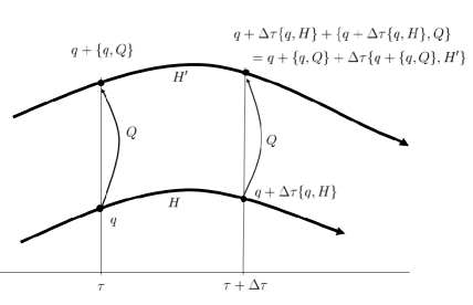
Figure 1: Time development in phase space

Let us consider an solution orbit, O₁, to the canonical equations of motion and its image, O₂, of a transformation generated by $Q\sim{\rm O}(\epsilon)$. Let $H^{\prime}$ be the time development generator of the mapped variable. Then from the equation written at the right-top of Fig.1, we see $\{q,H^{\prime}-H\}=\{q,\{H,Q\}\}+{\rm O}(\epsilon^{2})$, where the Jacobi identity is used. This means $H^{\prime}=H+\{H,Q\}$. If the transformtion is a CGTR, the new “hamiltonian” $H^{\prime}$ is differ from $H$ only by the Dirac variables. Assuming the two orbits cross at some point, they are physically equivalent. However, the set of physically equivalent orbits are wider than that obtained by CGTR.

A natural idea to incorporate the possible set of physically equivalent states might be treating the primary and the secondary constraints on the same footing. Thus Dirac made the conjecture that a transformation generated by linear combination of all 1st class constraints including secondary ones is a PETR. This amounts to assume that the hamiltonian defined by $H_{\rm E}=H+v_{i}\phi_{i}$ is the correct hamiltonian of the system, where $\phi_{i}$ are all 1st class constraints.

It seems hard to get the correct set of physically equivalent class of states along the above arguments. Therefore, in the present paper, based on the definition of the physical equivalence in the lagrangian theory and the relations of transformations between the lagrangian and the hamiltonian theories, we seek for the condition for a DTR to be PETR.

We assume that the initial point does not move under the transformations considered here. Then the PETR is the transformation which preserves LC’s and ELE’s. It is important to note that the meaning of the preservation above should be so relaxed that the two states represented by $(q,u)$ and $(q^{\prime},u^{\prime})$ satisfying $(q,u)\stackrel{{\scriptstyle\rm P}}{{\sim}}(q^{\prime},u^{\prime})$ defined in Section 2 are the same states. Therefore we define that a LTR satisfying

$$\delta_{\rm L}\ell \stackrel{{\scriptstyle\rm P}}{{\sim}} 0\qquad{\rm mod}~{}(\ell,{\rm[EM]}),$$ (4.4)

$$\delta_{\rm L}{\rm[EL]} \stackrel{{\scriptstyle\rm P}}{{\sim}} 0\qquad{\rm mod}~{}(\ell,{\rm[EM]}),$$ (4.5)

is PETR. In the phase space a HTR is defined to be PETR if the pull-back of it is PETR in the above sense. For the 1st order LC’s, the condition (4.4) is a special case of (4.5), while for 2nd and higher order LC’s those conditions are independent of (4.5).

Now let us seek for the condition that a DTR is PETR. Since a LC is the pull-back of a secondary constraint, we see, from (3.50),

$$\delta_{\rm L}\ell\Big{|}_{u=U_{\rm pb}}=\left[\{\chi,Q\}+\{\chi,Q^{\sim}\}_{\rm M}\right]_{\rm PB}\qquad{\rm mod}~{}(\ell,{\rm[EM]})(U_{\rm pb}),$$ (4.6)

where $\chi$ is the secondary constraint the pull-back of which is $\ell$.

Next let us calculate the the variation of ELE. From (3.50) we see

$$(\delta_{\rm L}W_{A})(U_{\rm pb})=[\delta_{Q}\pi_{A}+\{\pi_{A},Q^{\sim}\}_{\rm M}]_{\rm PB}\qquad{\rm mod}~{}(\ell,{\rm[EM]})(U_{\rm pb}).$$ (4.7)

Hence from (3.25)

$$\left(\frac{d}{d\tau}\delta_{\rm L}W_{A}\right)(q,U_{\rm pb})=[(\delta_{Q}\pi_{A})^{\sim}+\{\pi_{A},Q^{\sim}\}^{\sim}_{\rm M}]_{\rm PB}\qquad{\rm mod}~{}(\ell,{\rm[EM]})(U_{\rm pb}),$$ (4.8)

where mod $(\ell,{\rm[EM]})$ means that the equation holds if the quantities inside the bracket and their time derivatives vanish.

From (3.11) we see

$$\left(\frac{\partial{L}}{\partial{q^{A}}}\right)(U_{\rm pb})=-\left[\frac{\partial{H}}{\partial{q^{A}}}\right]_{\rm PB}.$$ (4.9)

Hence from (3.55)

$$\left(\delta_{\rm L}\frac{\partial{L}}{\partial{q^{A}}}\right)(U_{\rm pb})=-\left[\delta_{Q}\left(\frac{\partial{H}}{\partial{q^{A}}}\right)+\left\{\frac{\partial{H}}{\partial{q^{A}}},Q^{\sim}\right\}_{\rm EM}\right]_{\rm PB}{\rm mod}~{}(\ell,{\rm[EM]})(U_{\rm pb}).$$ (4.10)

From (4.8) and (4.10) we get

$$\delta_{\rm L}{\rm[EL]}_{A}(q,U_{\rm pb}) = \left[\frac{d}{d\tau}(\delta_{\rm L}W_{A})-\delta_{\rm L}\left(\frac{\partial{L}}{\partial{q^{A}}}\right)\right]_{u=U_{\rm pb}}$$

$$= \Big{[}\{\{\pi_{A},Q\},H\}+\{\{\pi_{A},Q^{\sim}\}_{\rm M},H\}$$

$$\qquad+\{\{H,\pi_{A}\},Q\}-\{\{\pi_{A},H\},Q^{\sim}\}_{\rm EM}\Big{]}_{\rm PB}\qquad{\rm mod}~{}(\ell,{\rm[EM]})(U_{\rm pb})$$

$$= \Big{[}\{\pi_{A},Q^{\sim}\}+\{\pi_{A},Q^{\sim}\}_{\rm M}^{\sim}-\{\pi_{A}{}^{\sim},Q^{\sim}\}_{\rm EM}\Big{]}_{\rm PB}\qquad{\rm mod}~{}(\ell,{\rm[EM]})(U_{\rm pb}),$$

where we used the Jacobi identity in the second line.

The function defined by $Q_{\xi}=\xi^{m}(q)\pi_{m}$ with infinitesimal parameters, $\xi^{m},~{}(m\geq R+1)$, generate a PETR. Thus we arrive at the conclusion that if there exist such $\xi^{m}$ that $\hat{Q}\stackrel{{\scriptstyle\rm{\small def}}}{{=}}Q_{\xi}+Q$ satisfies

$$\{\chi_{i},\hat{Q}\}+\{\chi_{i},\hat{Q}^{\sim}\}_{\rm M}=0\qquad{\rm mod}(\varphi,\chi),$$ (4.12)

for all secondary constraints, $\chi$’s, and

$$\{\pi_{A},\hat{Q}^{\sim}\}+\{\pi_{A},\hat{Q}^{\sim}\}_{\rm M}^{\sim}-\{\pi_{A}{}^{\sim},\hat{Q}^{\sim}\}_{\rm EM}=0\quad{\rm mod}~{}(\varphi,\chi),$$ (4.13)

then the DTR generated by $Q$ is PETR. (4.12) is the condition for the preservation of LC. If the constraints are closed not only with respect to Poisson bracket but with respect to M-bracket, then (4.12) is satisfied with $\xi^{m}=0$. Let us say that this kind of constraints belonging to class IA, and the DTR generated by them is of class IA DTR. The preservation of LC is automatically satisfied for class IA DTR. On the other hand (4.13) is the condition for the preservation of ELE, and it restricts the variation parameters along with the constraint structure.

Since two states which are described by the same coordinates, $(q^{A},u^{A})$, except that the $m$-components, $(q^{m},u^{m}),(m\geq R+1)$, are different from each other with finite values, are physically equivalent, we can extend the conditions (4.12) and (4.13) as

$$\qquad\left[\{\chi_{i},\hat{Q}\}+\{\chi_{i},\hat{Q}^{\sim}\}_{\rm M}\right]_{q^{m}=\Xi^{m}}=0\quad{\rm mod}(\varphi,\chi),$$ (4.14)

$$\left[\{\pi_{A},\hat{Q}^{\sim}\}+\{\pi_{A},\hat{Q}^{\sim}\}_{\rm M}^{\sim}-\{\pi_{A}{}^{\sim},\hat{Q}^{\sim}\}_{\rm EM}\right]_{q^{m}=\Xi^{m}}=0$$

$$\qquad\qquad\qquad\qquad\qquad\qquad{\rm mod}~{}(\varphi,\chi).$$ (4.15)

If there exist such $\Xi^{m}$, ($m\geq R+1$), that at $q^{m}=\Xi^{m}$ the above equations hold, then the DTR is PETR.

5 Examples

5.1 Maxwell model in $D$-dimensions

For the dynamical variables $q=(A^{i}(\mbox{\boldmath$x$}),A^{0}(\mbox{\boldmath$x$})),~{}u=(u^{i}(\mbox{\boldmath$x$}),u^{0}(\mbox{\boldmath$x$}))$ the lagrangian is

$$L = \int d^{D-1}x~{}{\cal L},$$

$${\cal L} = -\frac{1}{4}F_{\mu\nu}F^{\mu\nu}=\frac{1}{2}m_{ij}u^{i}u^{j}+n_{i}u^{i}+{\cal L}_{0},$$ (5.1)

where

$$m_{ij}=\delta_{ij},\qquad n_{i}=\partial_{i}A^{0},\qquad u^{i}=\partial_{0}A^{i},$$

$$\qquad{\cal L}_{0}=-\frac{1}{2}A^{0}\partial_{i}\partial^{i}A^{0}-\frac{1}{4}F_{ij}F^{ij}.$$ (5.2)

Here we use the metric convention: $\eta_{\mu\nu}={\rm diag}(-++\cdots+)$. We use the time variable $\tau=x^{0}$. $W$ and the Hessian are

$$W^{i}=u^{i}+\partial^{i}A^{0},\qquad W_{0}=0,$$

$$\quad M_{\mu\nu}(\mbox{\boldmath$x$},\mbox{\boldmath$x$}^{\prime})=\left(\begin{array}[]{cc}\delta_{ij}\delta^{D-1}(\mbox{\boldmath$x$}-\mbox{\boldmath$x$}^{\prime})&0\\ 0&0\end{array}\right).$$ (5.5)

ELE’s and the LC are

$$0 = {\rm[EL]}_{i}=\dot{u}_{i}-\partial_{i}u_{0}-\partial^{j}F_{ji},\qquad(i\leq D-1)$$ (5.6)

$$0 = {\rm[EL]}_{0}=\partial^{i}(u_{i}-\partial_{i}A_{0})\stackrel{{\scriptstyle\rm{\small def}}}{{=}}\ell,\qquad({\rm LC})$$ (5.7)

$$0 = \dot{A}^{\mu}-u^{\mu}.$$ (5.8)

From (5.6), $\dot{\ell}$ vanishes, hence 2nd and higher order LC’s are absent. The LC, (5.7), is the Gauss law, and is the Poisson equation for $A_{0}$, which has the unique solution if one sets a boundary condition for $A_{0}$. However, the time derivative $u_{0}=\dot{A}_{0}$ are arbitrary, and according to our definition, $A_{0}$ is an unphysical variable.

Under the transformation

$$\delta A_{i}=\partial_{i}\varepsilon,\qquad\delta A_{0}=\eta,\qquad\delta u_{\mu}=\frac{d}{d\tau}(\delta A_{\mu})$$ (5.9)

with arbitrary parameters, $\varepsilon(\mbox{\boldmath$x$},\tau),\eta(\mbox{\boldmath$x$},\tau)$, the lagrangian varies as

$$\delta L=\int d^{D-1}x~{}(\eta-\dot{\varepsilon})\ell+{\rm T.D.}.$$ (5.10)

Hence (5.9) is a LTR, and also is a SGTR.

Primary constraint in the canonical theory is

$$\varphi\stackrel{{\scriptstyle\rm{\small def}}}{{=}}\pi_{0}=0.$$ (5.11)

The general solution to $\pi=W$ is

$$\hat{U}^{i}=\pi^{i}-\partial^{i}A^{0},\qquad\hat{U}^{0}=\theta(A,\pi),$$ (5.12)

where $\theta$ is an arbitrary function. Using them, hamiltonian is given by

$$H=\int d^{D-1}x~{}\left(\frac{1}{2}\pi_{i}\pi^{i}+\frac{1}{4}F_{ij}F^{ij}+A^{0}\chi+\theta\varphi\right),$$ (5.13)

where

$$\chi\stackrel{{\scriptstyle\rm{\small def}}}{{=}}\partial_{i}\pi^{i}.$$ (5.14)

1st order secondary constraint is $\chi=0$, and 2nd and higher order secondary constraints are absent.

The canonical equations of motion are

$$\dot{A}^{i}=\pi^{i}-\partial^{i}A^{0},\qquad\dot{A^{0}}=\theta(A,\pi),\qquad\dot{\pi}_{i}=\partial^{j}F_{ji}\qquad\dot{\pi}_{0}=-\partial_{i}\pi^{i}.$$ (5.15)

Substituting $\pi^{\mu}=W^{\mu}(A,u)$ into the above equations, we get the pull-back of them as

$$\dot{A}^{i}=u^{i},\qquad\dot{A}^{0}=\theta(A,W(A,u)),\qquad\dot{u}_{i}=\partial_{i}\dot{A}_{0}+\partial^{j}F_{ji},\qquad\ell=0.$$ (5.16)

If we write

$$U_{\rm pb}\stackrel{{\scriptstyle\rm{\small def}}}{{=}}\theta(A,W(A,u)),$$ (5.17)

then (5.16) coincide with the Euler-Lagrange equations, the relations $\dot{A}^{\mu}-u^{\mu}=0$ and the LC, expressed in (5.6) $\sim$ (5.8), where $u^{0}$ is replaced by $U_{\rm pb}$.

Writing a generator of DTR as

$$Q=-\int d^{D-1}x~{}(\epsilon\chi+\eta\varphi),$$ (5.18)

we have

$$\delta_{Q}A_{i}=\partial_{i}\epsilon,\qquad\delta_{Q}A_{0}=\eta,$$ (5.19)

$$Q^{\sim}=-(\epsilon^{\sim}-\eta)\chi\qquad{\rm mod}~{}\varphi.$$ (5.20)

If $\eta=\epsilon^{\sim}$ the HTR generated by $Q$ is CGTR, and the pull-back of it is the GTR, $\delta_{\rm L}A_{\mu}=\partial_{\mu}\epsilon.$

The constraints, $\varphi$ and $\chi$, are of 1st class, but they do not close with respect to M-bracket, hence do not belong to class IA. Putting $\hat{Q}=\xi\pi_{0}+Q$, we have

$$\{\chi,\hat{Q}\}+\{\chi,\hat{Q}^{\sim}\}_{\rm M}=\Delta(\epsilon^{\sim}-\eta-\xi)\qquad~{}~{}{\rm mod}~{}(\varphi,\chi),$$ (5.21)

$$\{\pi_{i},\hat{Q}^{\sim}\}+\{\pi_{i},\hat{Q}^{\sim}\}_{\rm M}^{\sim}-\{\pi_{i}{}^{\sim},\hat{Q}^{\sim}\}_{\rm EM}=\partial_{i}(\epsilon^{\sim}-\eta-\xi)^{\sim}\qquad{\rm mod}~{}(\varphi,\chi).$$ (5.22)

Hence the conditions for PETR, expressed in (4.12)-(4.13), are satisfied by choosing $\xi=\epsilon^{\sim}-\eta$. Thus we see every DTR in the Maxwell model is PETR.

5.2 Relativistic particle

Dynamical variables of relativistic particle with mass $m$ in $D$-dimensional Minkowski spacetime are the coordinate $x^{\mu},(\mu=0,1,,..,D-1)$, and the velocity variables $u^{\mu},(\mu=0,1,,..,D-1)$. We use the vector notation in $D$-dimensions as $\mbox{\boldmath$x$},\mbox{\boldmath$u$}$. The lagrangian is

$$L=\frac{1}{2e}\mbox{\boldmath$u$}^{2}-\frac{1}{2}m^{2}e,$$ (5.23)

where $e$ is the einbein and $\tau$ parametrizes an orbit of the particle. Including the einbein we write the coordinate and the velocity variables as $q^{A}=(x^{\mu},e)$ and $u^{A}=(u^{\mu},u)$, respectively.

Hessian and $W$ are

$$M_{AB}=\left(\begin{array}[]{cc}\frac{1}{e}\eta_{\mu\nu}&0\\ 0&0\end{array}\right),\qquad W_{A}=\left(\begin{array}[]{c}\frac{1}{e}u_{\mu}\\ 0\end{array}\right).$$ (5.28)

ELE and 1st order LC are

$${\bf[EL]}\stackrel{{\scriptstyle\rm{\small def}}}{{=}}\frac{d}{d\tau}\left(\frac{\mbox{\boldmath$u$}}{e}\right)=0,\qquad\ell\stackrel{{\scriptstyle\rm{\small def}}}{{=}}\frac{1}{2}\left(\frac{\mbox{\boldmath$u$}^{2}}{e^{2}}+m^{2}\right),=0.$$ (5.29)

2nd and higher order LC’s are absent. If $m\neq 0$ the LC can be solved for $e$ as $e=\sqrt{-\mbox{\boldmath$u$}^{2}}/m$, and substituting it back into the lagrangian we get the usual action $I=\int d\tau L=-m\int\sqrt{-d\mbox{\boldmath$x$}^{2}}$. Lagrangian of the form (5.23) is useful, since it can be used even in the case of $m=0$. The einbein, $e$, is unphysical because the lagrangian does not contain $u=\dot{e}$.

Under the transformation,

$$\delta\mbox{\boldmath$x$}=\epsilon\mbox{\boldmath$u$},\quad\delta e=\eta,\quad\delta\mbox{\boldmath$u$}=\frac{d}{d\tau}\delta\mbox{\boldmath$x$},\quad\delta u=\frac{d}{d\tau}\delta e,$$ (5.30)

with arbitrary $\epsilon$ and $\eta$, the lagrangian varies as

$$\delta L=\left(\frac{d}{d\tau}(e\epsilon)-\eta\right)\ell+\frac{d}{d\tau}(\epsilon L).$$ (5.31)

Hence the transformation is a LTR, and also is a SGTR.

Writing the canonical momenta of $x$ and $e$ as $\pi$ and $\pi$, respectively, the primary constraint is

$$\varphi\stackrel{{\scriptstyle\rm{\small def}}}{{=}}\pi=0.$$ (5.32)

The general solution for $u_{A}$ to equation $\pi_{A}=W_{A}(\mbox{\boldmath$x$},e,\mbox{\boldmath$u$},u)$ is

$$\mbox{\boldmath$u$}=\hat{\mbox{\boldmath$U$}}\stackrel{{\scriptstyle\rm{\small def}}}{{=}}e\mbox{\boldmath$\pi$},\qquad u=\hat{U}\stackrel{{\scriptstyle\rm{\small def}}}{{=}}\theta(\mbox{\boldmath$x$},\mbox{\boldmath$\pi$},e,p),$$ (5.33)

where $\theta$ is an arbitrary function. Using them the hamiltonian is written as

$$H=e\chi+\theta\pi,\qquad\chi\stackrel{{\scriptstyle\rm{\small def}}}{{=}}\frac{1}{2}(\mbox{\boldmath$\pi$}^{2}+m^{2}).$$ (5.34)

1st order secondary constraint is $\chi=0$, and 2nd order and higher order secondary constraints are absent.

The canonical equations of motion are

$$\dot{x}^{i}=e\pi^{i},\quad\dot{e}=\theta,\quad\dot{\pi}_{i}=0\quad{\rm mod}~{}\varphi,\quad\dot{\pi}=-\chi.$$ (5.35)

Substituting $\pi_{i}=u_{i}/e,~{}\pi=0$ into the above equations, we get the pull-back of them as

$$\frac{d}{d\tau}\left(\frac{u^{i}}{e}\right)=0,\quad\chi=0,\quad\dot{x}^{i}=u^{i},\quad\dot{e}=\theta.$$ (5.36)

If we write $u^{\prime}\stackrel{{\scriptstyle\rm{\small def}}}{{=}}\theta(q,W(q,u))$, then (5.36) coincide with the ELEs, the relations $\dot{q}^{A}-u^{A}=0$ and the LC, where $u$’s are replaced by $u^{\prime}$’s.

Writing a generator of DTR as

$$Q=\varepsilon\chi+\eta\varphi,$$ (5.37)

we have

$$\delta_{Q}\mbox{\boldmath$x$}=\varepsilon\mbox{\boldmath$\pi$},\qquad\delta_{Q}e=\eta,$$ (5.38)

$$Q^{\sim}=(\varepsilon^{\sim}-\eta)\chi\quad{\rm mod}~{}\varphi.$$ (5.39)

Putting $\hat{Q}=\xi\pi+Q$, we see

$$\{\chi,\hat{Q}\}+\{\chi,\hat{Q}^{\sim}\}_{\rm M}=(\varepsilon^{\sim}-\eta-\xi)\mbox{\boldmath$\pi$}^{2},\qquad{\rm mod}(\varphi,\chi)$$ (5.40)

$$\{\mbox{\boldmath$\pi$},\hat{Q}^{\sim}\}+\{\mbox{\boldmath$\pi$},\hat{Q}^{\sim}\}_{\rm M}-\{\mbox{\boldmath$\pi$}^{\sim},\hat{Q}^{\sim}\}_{\rm EM}^{\sim}=\left(\frac{1}{e}(\varepsilon^{\sim}-\eta-\xi)\mbox{\boldmath$\pi$}\right)^{\sim}\qquad{\rm mod}(\varphi,\chi).$$ (5.41)

In the massless case, the constraints, $\varphi$ and $\chi$ close with respect to M-bracket, so belong to class IA, while in the massive case, they do not. For both cases, the conditions for PETR, (4.12) and (4.13), are satisfied by choosing $\xi=\varepsilon^{\sim}-\eta$. Thus we see every DTR of the relativistic particle is PETR.

5.3 Bilocal particle

The model consists of two relativistic particles, and hidden symmetries extending the reparametrizations and a global symmetry were found[7]. Dynamical variables are $q=(x^{\mu}_{k},e_{k}),~{}u=(u^{\mu}_{k},u_{k}),~{}(k=1,2)$ , and lagrangian is

$$L=\frac{1}{2e_{1}}\mbox{\boldmath$u$}_{1}\cdot\mbox{\boldmath$u$}_{1}+\frac{1}{2e_{2}}\mbox{\boldmath$u$}_{2}\cdot\mbox{\boldmath$u$}_{2}+\kappa(\mbox{\boldmath$u$}_{1}\cdot\mbox{\boldmath$x$}_{2}-\mbox{\boldmath$u$}_{2}\cdot\mbox{\boldmath$x$}_{1}),$$ (5.42)

where $\kappa$ is a parameter of the model with dimension of mass square. ELE’s and LC’s are

$${\bf[EL]}_{k}\stackrel{{\scriptstyle\rm{\small def}}}{{=}}\frac{d}{d\tau}\left(\frac{\mbox{\boldmath$u$}_{k}}{e_{k}}-2\kappa s_{k}\mbox{\boldmath$x$}_{k^{\prime}}\right)=\mbox{\boldmath$0$},\quad({\rm ELE})$$ (5.43)

$$\ell_{k}\stackrel{{\scriptstyle\rm{\small def}}}{{=}}\mbox{\boldmath$u$}_{k}\cdot\mbox{\boldmath$u$}_{k}=0,\qquad(k=1,2)\quad\quad({\rm LC})$$ (5.44)

$$\mbox{\boldmath$u$}_{k}=\dot{\mbox{\boldmath$x$}}_{k},\qquad u_{k}=\dot{e}_{k},\qquad(k=1,2)$$ (5.45)

where we put

$$s_{k}\stackrel{{\scriptstyle\rm{\small def}}}{{=}}(-1)^{k},\qquad k^{\prime}\stackrel{{\scriptstyle\rm{\small def}}}{{=}}3-k.$$ (5.46)

Hessian and $W$ are

$$M_{AB}=\left(\begin{array}[]{cc}\frac{1}{e_{k}}\delta_{jk}\eta_{\mu\nu}&0\\ 0&0\end{array}\right),$$ (5.49)

$$\qquad\mbox{\boldmath$W$}_{k}=\frac{\mbox{\boldmath$u$}_{k}}{e_{k}}-\kappa s_{k}\mbox{\boldmath$x$}_{k^{\prime}},\qquad W_{k}=0.$$ (5.50)

Using (5.43), the time derivative of $\ell_{k}$ are given as

$$\dot{\ell}_{k}=4\kappa e_{k}s_{k}\mbox{\boldmath$u$}_{1}\cdot\mbox{\boldmath$u$}_{2}\qquad{\rm mod}~{}{\rm[EL]}.$$ (5.51)

Hence if $\kappa\neq 0$ we have a 2nd order LC,

$$\ell_{0}\stackrel{{\scriptstyle\rm{\small def}}}{{=}}\mbox{\boldmath$u$}_{1}\cdot\mbox{\boldmath$u$}_{2}=0.$$ (5.52)

3rd and higher order lagrangian constraints are absent. Since the lagrangian does not contain, the variables $e_{k},(k=1,2)$ are unphysical.

Under the transformation defined by

$$\delta_{\rm L}\mbox{\boldmath$x$}_{k}=\varepsilon_{k}\mbox{\boldmath$u$}_{k}+\frac{\varepsilon_{0}}{e_{k^{\prime}}}\mbox{\boldmath$u$}_{k^{\prime}},\qquad\delta_{\rm L}e_{k}=\eta_{k},$$ (5.53)

$$\quad\delta\mbox{\boldmath$u$}_{k}=\frac{d}{d\tau}\delta\mbox{\boldmath$x$}_{k},\qquad\delta u_{k}=\frac{d}{d\tau}\delta e_{k},\qquad\qquad$$ (5.54)

the lagrangian varies as

$$\delta L=\frac{1}{2}\left(\frac{d}{d\tau}(\varepsilon_{k}e_{k})-4\kappa s_{k}\varepsilon_{0}e_{k}-\eta_{k}\right)\ell_{k}+\frac{\dot{\varepsilon}_{0}-2\kappa e_{1}e_{2}(\varepsilon_{1}-\varepsilon_{2})}{e_{1}e_{2}}\ell_{0}+{\rm T.D.}.\qquad$$ (5.55)

Hence the transformation is LTR, and also is SGTR.

Denoting the canonical conjugates to $\mbox{\boldmath$x$}_{k},~{}e_{k},(k=1,2)$ as $\mbox{\boldmath$\pi$}_{k},~{}\pi_{k},(k=1,2)$, the primary constraints in the canonical theory are

$$\varphi_{m}\stackrel{{\scriptstyle\rm{\small def}}}{{=}}\pi_{m}=0.\qquad(m=1,2)$$ (5.56)

The general solutions of $\mbox{\boldmath$u$}_{k}=\hat{\mbox{\boldmath$U$}}_{k},~{}u_{k}=\hat{U}_{k},~{}(k=1,2)$ to the equations $\pi_{A}=W_{A}(q,u)$ are

$$\hat{\mbox{\boldmath$U$}}_{k}=e_{k}(\mbox{\boldmath$\pi$}_{k}+\kappa s_{k}\mbox{\boldmath$x$}_{k^{\prime}}),\qquad\hat{U}_{k}=\theta_{k}(\mbox{\boldmath$x$},\mbox{\boldmath$\pi$},e,\pi),$$ (5.57)

where $\theta_{k}$ are arbitrary functions. Using them the hamiltonian is written as

$$H=e_{k}\chi_{k}+\theta_{k}\pi_{k},\quad\chi_{k}\stackrel{{\scriptstyle\rm{\small def}}}{{=}}\frac{1}{2}(\mbox{\boldmath$\pi$}_{k}+\kappa s_{k}\mbox{\boldmath$x$}_{k^{\prime}})^{2},\quad(k=1,2).$$ (5.58)

1st order secondary constraints are $\chi_{1}=\chi_{2}=0$, and if $\kappa\neq 0$ there is a 2nd order secondary constraint,

$$\chi_{0}\stackrel{{\scriptstyle\rm{\small def}}}{{=}}(\mbox{\boldmath$\pi$}_{1}-\kappa\mbox{\boldmath$x$}_{2})\cdot(\mbox{\boldmath$\pi$}_{2}+\kappa\mbox{\boldmath$x$}_{1})=0,$$ (5.59)

while 3rd and higher order secondary constraints are absent. The pull-backs of the three secondary constraints, $\chi_{i}=0,(i=0,1,2)$, are equivalent to the three LCs, $\ell_{i}=0,(i=0,1,2)$. Note that no $\chi_{0}$ term exists in the hamiltonian.

The Poisson brackets between $\chi_{i},(i=0,1,2)$ are

$$\{\chi_{1},\chi_{2}\}=-2\kappa\chi_{0},\quad\{\chi_{k},\chi_{0}\}=4\kappa s_{k}\chi_{k}\quad(k=1,2).\quad$$ (5.60)

Using the normalised basis defined by $\chi^{\prime}_{1}=\chi_{1}/2\kappa,~{}\chi^{\prime}_{-1}=\chi_{2}/2\kappa,~{}\chi^{\prime}_{0}=-\chi_{0}/4\kappa$, the Poisson brackets gives the familiar $sl(2,\mathbb{R})$ algebra:

$$\{\chi^{\prime}_{n},\chi^{\prime}_{m}\}=(n-m)\chi^{\prime}_{n+m}.\qquad(n,m=0,\pm 1)$$ (5.61)

The canonical equations of motion are

$$\dot{\mbox{\boldmath$x$}}_{k}=\hat{\mbox{\boldmath$U$}}_{k},\qquad\dot{e}_{k}=\theta_{k},$$ (5.62)

$$\dot{\mbox{\boldmath$\pi$}}_{k}=-e_{k^{\prime}}(\mbox{\boldmath$\pi$}_{k^{\prime}}+\kappa s_{k^{\prime}}\mbox{\boldmath$x$}_{k}).$$ (5.63)

Using (5.62), (5.63) can be written in terms of $\hat{\mbox{\boldmath$U$}}_{k}$ as

$$\frac{d}{d\tau}\left(\frac{\hat{\mbox{\boldmath$U$}}_{k}}{e_{k}}-2\kappa s_{k}\mbox{\boldmath$x$}_{k^{\prime}}\right)=0,$$ (5.64)

which, along with (5.62), coincide with the ELE’s and the relations $\dot{q}^{A}-u^{A}=0$, expressed in (5.43) and (5.45), where $u$ and $u$ are replaced by $\hat{\mbox{\boldmath$U$}}$ and $\theta$, respectively.

Wtiting a generator of DTR as

$$Q=\epsilon_{0}\chi_{0}+\epsilon_{k}e_{k}\chi_{k}+\eta_{k}\pi_{k},$$ (5.65)

we have

$$\delta_{Q}\mbox{\boldmath$x$}_{k}=\epsilon_{k}e_{k}(\mbox{\boldmath$\pi$}_{k}+\kappa s_{k}\mbox{\boldmath$x$}_{k^{\prime}})+\epsilon_{0}(\mbox{\boldmath$\pi$}_{k^{\prime}}-\kappa s_{k}\mbox{\boldmath$x$}_{k}),\quad\delta_{Q}\mbox{\boldmath$\pi$}_{k}=\kappa s_{k}\delta\mbox{\boldmath$x$}_{k^{\prime}},\quad\delta_{Q}e_{k}=\eta_{k},$$ (5.66)

$$Q^{\sim}=A_{k}\chi_{k}+A_{0}\chi_{0}\qquad{\rm mod}~{}\varphi,$$ (5.67)

$$A_{k}\stackrel{{\scriptstyle\rm{\small def}}}{{=}}(\epsilon_{k}e_{k})^{\sim}-4\kappa s_{k}e_{k}\epsilon_{0}-\eta_{k},\qquad A_{0}\stackrel{{\scriptstyle\rm{\small def}}}{{=}}\epsilon_{0}{}^{\sim}-2\kappa e_{1}e_{2}(\epsilon_{1}-\epsilon_{2}).$$ (5.68)

M-brackets among the constraints are

$$\{\varphi_{i},\varphi_{j}\}_{\rm M}=\{\varphi_{i},\chi_{j}\}_{\rm M}=\{\varphi_{i},\chi_{0}\}_{\rm M}=0,\qquad(i,j=1,2)$$ (5.69)

$$\{\chi_{i},\chi_{j}\}_{\rm M}=\frac{1}{e_{i}}\delta_{ij}\chi_{i},\qquad\{\chi_{0},\chi_{i}\}_{\rm M}=\frac{1}{e_{i}}\chi_{0},\qquad\{\chi_{0},\chi_{0}\}_{\rm M}=\sum_{i=1}^{2}\frac{\chi_{i}}{e_{i}},$$ (5.70)

hence the constraints are of class IA. Thus the preservation of the LCs are satisfied automatically. The preservation of ELE, are written as

$$\{\mbox{\boldmath$\pi$},\hat{Q}^{\sim}\}+\{\mbox{\boldmath$\pi$},\hat{Q}^{\sim}\}_{\rm M}^{\sim}-\{\mbox{\boldmath$\pi$}^{\sim},\hat{Q}^{\sim}\}_{\rm EM}$$

$$\qquad=\left[(A_{k}-\xi_{k})\frac{\hat{\mbox{\boldmath$U$}}_{k}}{e_{k}^{2}}+A_{0}\frac{\hat{\mbox{\boldmath$U$}}_{k^{\prime}}}{e_{1}e_{2}}\right]^{\sim}=0\quad{\rm mod}~{}(\varphi,\chi)\qquad~{}~{}$$ (5.71)

with $\hat{Q}=\xi^{m}\pi_{m}+Q$. The first term in the parenthesis of r.h.s. can be zero by choosing $\xi_{k}=A_{k},(k=1,2)$, while the second term can be zero if, using the extended conditions for PETR,

$$\epsilon_{0}{}^{\sim}-2\kappa\Xi_{1}\Xi_{2}(\epsilon_{1}-\epsilon_{2})=0.$$ (5.72)

Since $\Xi_{k}$ are arbitrary, the above equation can be satisfied for arbitrary $\epsilon_{i},(i=0,1,2)$ except the case of $\epsilon_{1}=\epsilon_{2}$. Therefore we get the conclusion that a DTR in the bilocal particle model is a PETR, except the transformation with $\epsilon_{1}=\epsilon_{2}$.

5.4 Cawley model

As a counter-example to Dirac’s conjecture Cawley found the following model [3, 4]. Dynamical variables are $(q_{1},q_{2},q_{3})$ and the corrensponding velocity $(u_{1},u_{2},u_{3})$, and lagrangian is

$$L=u_{1}u_{2}-\frac{1}{2}q_{3}(q_{2})^{2}.$$ (5.73)

ELE’s and 1st order LC are

$${\rm[EL]}_{1}\stackrel{{\scriptstyle\rm{\small def}}}{{=}}\dot{u}_{2}=0,\qquad{\rm[EL]}_{2}\stackrel{{\scriptstyle\rm{\small def}}}{{=}}\dot{u}_{1}+q_{3}q_{2}=0,\qquad$$ (5.74)

$$\ell_{1}\stackrel{{\scriptstyle\rm{\small def}}}{{=}}q_{2}=0.$$ (5.75)

There is a 2nd order LC,

$$\ell_{2}\stackrel{{\scriptstyle\rm{\small def}}}{{=}}u_{2}=0,$$ (5.76)

while 3rd and higher order lagrangian constraints are absent. $W$ and Hessian are

$$W_{1}=u_{2},\qquad W_{2}=u_{1},\qquad W_{3}=0,\qquad M_{ij}=\left(\begin{array}[]{ccc}0&1&0\\ 1&0&0\\ 0&0&0\end{array}\right).$$ (5.80)

Since the lagrangian does not contain $u_{3}$, the variable $q_{3}$ is unphysical.

Under the transformation

$$\delta q_{1}=\epsilon_{2},\qquad\delta q_{2}=0,\qquad\delta q_{3}=\eta,$$ (5.81)

lagrangian varies as

$$\delta L=-\ddot{\epsilon}_{2}\ell_{1}+{\rm T.D.},$$ (5.82)

where O$(\ell_{1})^{2}$ term is dropped. Hence the transformation is LTR, and is also SGTR.

Denoting the canonical momenta corresponding to $q_{i},(i=1,2,3)$ as $\pi_{i},(i=1,2,3)$, the primary constraint is

$$\varphi\stackrel{{\scriptstyle\rm{\small def}}}{{=}}\pi_{3}=0.$$ (5.83)

The general solution for $u$’s to the equations $\pi_{i}=W_{i}(q,u)$ is

$$u_{1}=\hat{U}_{1}\stackrel{{\scriptstyle\rm{\small def}}}{{=}}\pi_{2},\quad u_{2}=\hat{U}_{2}\stackrel{{\scriptstyle\rm{\small def}}}{{=}}\pi_{1},\quad u_{3}=\hat{U}_{3}\stackrel{{\scriptstyle\rm{\small def}}}{{=}}\theta,$$ (5.84)

where $\theta$ is an arbitrary function. Using them, hamiltonian is written as

$$H=\pi_{2}\chi_{2}+\frac{1}{2}q_{3}(\chi_{1})^{2}+\theta\varphi,\quad\chi_{1}\stackrel{{\scriptstyle\rm{\small def}}}{{=}}q_{2},\quad\chi_{2}\stackrel{{\scriptstyle\rm{\small def}}}{{=}}\pi_{1}.$$ (5.85)

1st order secondary constraint is $\chi_{1}=0.$ There is a 2nd order secondary constraint, $\chi_{2}=0,$ while 3rd and higher order secondary constraints are absent. The pull-back of $\chi_{1}$ and $\chi_{2}$ are $\ell_{1}$ and $\ell_{2}$, respectively.

Canonical equations of motion are

$$\dot{q}_{1}=\pi_{2},\quad\dot{q}_{2}=\chi_{2},\quad\dot{q}_{3}=\theta,$$ (5.86)

$$\dot{\pi}_{1}=0,\quad\dot{\pi}_{2}=-q_{3}\chi_{1},\quad\dot{\pi}_{3}=-\frac{1}{2}\chi_{1}^{2}.\qquad$$ (5.87)

Writing the generating function $Q$ of DTR as

$$Q=\epsilon_{1}\chi_{1}+\epsilon_{2}\chi_{2}+\eta\varphi,$$ (5.88)

we see

$$\delta_{Q}q_{1}=\epsilon_{2},\quad\delta_{Q}q_{2}=0,\quad\delta_{Q}q_{3}=\eta,$$ (5.89)

$$\delta_{Q}\pi_{1}=0,\quad\delta_{Q}\pi_{2}=-\epsilon_{1}\quad\delta_{Q}\pi_{3}=0,$$ (5.90)

$$Q^{\sim}=\epsilon_{1}{}^{\sim}\chi_{1}+(\epsilon_{2}{}^{\sim}+\epsilon_{1})\chi_{2}-\frac{1}{2}\eta(\chi_{1})^{2}\quad{\rm mod}~{}\varphi.\qquad$$ (5.91)

All M-brackets among the constraints vanish, i.e., they are of class IA. Hence the preservation of the LC holds automatically. On the other hand, the preservation of ELE is written, for example, as

$$\{\pi_{2},Q^{\sim}\}+\{\pi_{2},Q^{\sim}\}_{\rm M}^{\sim}-\{\pi_{2}{}^{\sim},Q^{\sim}\}_{\rm EM}=\epsilon_{2}{}^{\sim\sim}~{}~{}{\rm mod}~{}(\varphi,\chi),~{}~{}$$ (5.92)

which does not vanish. R.h.s. of the above equation does not change even if we add $\xi\pi_{3}$ term to $Q$. Thus we find that the DTR is not a PETR, i.e., Dirac’s conjecture in the Cawley model does not hold.

5.5 Frenkel model

A slightly differnt model from Cawley’s one was discussed by Frenkel [5]. The kinetic term of the lagrangian is changed to be 3rd power of the velocity variables, i.e.,

$$L=u_{1}(u_{2})^{2}-\frac{1}{2}q_{3}(q_{2})^{2}.$$ (5.93)

ELE’s are changed as

$${\rm[EL]}_{1}\stackrel{{\scriptstyle\rm{\small def}}}{{=}}2u_{2}\dot{u}_{2}=0,\quad{\rm[EL]}_{2}\stackrel{{\scriptstyle\rm{\small def}}}{{=}}2\frac{d}{d\tau}(u_{1}u_{2})+q_{3}q_{2}=0.$$ (5.94)

The 1st and the 2nd order LC’s are the same as those of Cawley model, i.e., $\ell_{1}\stackrel{{\scriptstyle\rm{\small def}}}{{=}}q_{2}=0,~{}\ell_{2}\stackrel{{\scriptstyle\rm{\small def}}}{{=}}u_{2}=0.$ Hessian and $W$ are

$$W_{1}=(u_{2})^{2},\qquad W_{2}=2u_{1}u_{2},\qquad W_{3}=0,\qquad M_{ij}=\left(\begin{array}[]{ccc}0&2u_{2}&0\\ 2u_{2}&2u_{1}&0\\ 0&0&0\end{array}\right).$$ (5.98)

Under the transformation

$$\delta q_{1}=\epsilon_{2},\qquad\delta q_{2}=0,\qquad\delta q_{3}=\eta,$$ (5.99)

the lagrangian varies as

$$\delta L=\dot{\epsilon}_{2}(\ell_{2})^{2}-\frac{1}{2}\eta(\ell_{1})^{2},$$ (5.100)

hence the transformation is LTR, and also a SGTR.

The primary constraint is the same as that of Cawley model:

$$\varphi\stackrel{{\scriptstyle\rm{\small def}}}{{=}}\pi_{3}=0.$$ (5.101)

The general solution for $u$’s to the equations $\pi_{i}=W_{i}(q,u)$ is

$$u_{1}=\hat{U}_{1}\stackrel{{\scriptstyle\rm{\small def}}}{{=}}\frac{\pi_{2}}{2\sqrt{\pi_{1}}},\quad u_{2}=\hat{U}_{2}\stackrel{{\scriptstyle\rm{\small def}}}{{=}}\sqrt{\pi_{1}},\quad u_{3}=\hat{U}_{3}\stackrel{{\scriptstyle\rm{\small def}}}{{=}}\theta.~{}~{}$$ (5.102)

Using them hamiltonian is written as

$$H=\pi_{2}\sqrt{\pi_{1}}+\frac{1}{2}q_{3}(q_{2})^{2}+\theta\varphi.$$ (5.103)

1st and 2nd order secondary constraints are the same as those of Cawley model:

$$\chi_{1}\stackrel{{\scriptstyle\rm{\small def}}}{{=}}q_{2}=0,\qquad\chi_{2}\stackrel{{\scriptstyle\rm{\small def}}}{{=}}\pi_{1}=0.$$ (5.104)

Hamiltonian is written in terms of the constraints as

$$H=\pi_{2}(\chi_{2})^{2}+\frac{1}{2}q_{3}(\chi_{1})^{2}+\theta\varphi,$$ (5.105)

where the 1st term in r.h.s. of the above equation is different from that of Cawley model.

Writing the generating function $Q$ of DTR as

$$Q=\epsilon_{1}\chi_{1}+\epsilon_{2}\chi_{2}+\eta\varphi,$$ (5.106)

we see

$$\delta_{Q}q_{1}=\epsilon_{2},\qquad\delta_{Q}q_{2}=0,\qquad\delta_{Q}q_{3}=\eta,$$ (5.107)

$$\delta_{Q}\pi_{1}=0,\qquad\delta_{Q}\pi_{2}=-\epsilon_{1}\qquad\delta_{Q}\pi_{3}=0,$$ (5.108)

$$Q^{\sim}=\epsilon_{1}{}^{\sim}\chi_{1}+\epsilon_{2}{}^{\sim}\chi_{2}+\epsilon_{1}(\chi_{2})^{2}-\frac{1}{2}\eta(\chi_{1})^{2}\quad{\rm mod}~{}\varphi.\qquad~{}~{}$$ (5.109)

The preservation of the LC’s holds automatically as in the case of Cawley model. The preservation of the ELE’s holds also,

$$\{\pi_{i},Q^{\sim}\}+\{\pi_{i},Q^{\sim}\}_{\rm M}^{\sim}-\{\pi_{i}{}^{\sim},Q^{\sim}\}_{\rm EM}=0\qquad{\rm mod}~{}(\varphi,\chi),$$ (5.110)

which is not the case in the Cawley model. Thus we find that the DTR is a PETR, i.e., Dirac’s conjecture holds in the Frenkel model.

5.6 Polyakov string

Dynamical variables of the string are the coordinates, $x^{\mu},~{}(\mu=0,1,..,D-1)$, of the string in the $D$-dimensional target space. These variables are functions of 2-dimensional coordinates, $(\sigma,\tau)$, and the model is regarded as a 2-dimensional field theory. The velocity variables, $u^{\mu}$, are the $\tau$-derivatives of $x^{\mu}$. Lagrangian is written in the Polyakov form,

$$L = \frac{1}{2}\int d\sigma~{}\sqrt{g}g^{\alpha\beta}\partial_{\alpha}\mbox{\boldmath$x$}\cdot\partial_{\beta}\mbox{\boldmath$x$},$$ (5.111)

where $g_{\alpha\beta}$ is the world sheet metric ($g\stackrel{{\scriptstyle\rm{\small def}}}{{=}}\det{g_{\alpha\beta}}>0$), and $x$ is the $D$-dimensional vector with the components, $(\mbox{\boldmath$x$})^{\mu}=x^{\mu}$. Since the 2-dimensional theory has the scale invariance, the lagrangian is written in terms of two variables among the three components of $g_{\alpha\beta}$. In fact, denoting $a=g^{00}\sqrt{g},~{}b=g^{01}\sqrt{g}$, the lagrangian is written as

$$L=\int d\sigma\left(\frac{1}{2}a\mbox{\boldmath$u$}^{2}+b\mbox{\boldmath$u$}\cdot\mbox{\boldmath$x$}^{\prime}+\frac{1+b^{2}}{2a}\mbox{\boldmath$x$}^{\prime 2}\right),$$ (5.112)

where $\mbox{\boldmath$u$}=\dot{\mbox{\boldmath$x$}}$ and $\mbox{\boldmath$x$}^{\prime}$ are the derivatives of $x$ with respect to $\tau$ and $\sigma$, respectively. Since the lagrangin does not contain the velocity variables corresponding to $a$ and $b$, these variables are unphysical.

ELE’s and 1st order LC’s are

$${\bf[EL]}\stackrel{{\scriptstyle\rm{\small def}}}{{=}}\frac{d}{d\tau}(a\mbox{\boldmath$u$}+b\mbox{\boldmath$x$}^{\prime})+\left(b\mbox{\boldmath$u$}+\frac{1+b^{2}}{a}\mbox{\boldmath$x$}^{\prime}\right)^{\prime}=0,$$ (5.113)

$$\ell_{1}\stackrel{{\scriptstyle\rm{\small def}}}{{=}}a^{2}\mbox{\boldmath$u$}^{2}-(1+b^{2})\mbox{\boldmath$x$}^{\prime 2}=0,\quad\ell_{2}\stackrel{{\scriptstyle\rm{\small def}}}{{=}}a\mbox{\boldmath$u$}\cdot\mbox{\boldmath$x$}^{\prime}+b\mbox{\boldmath$x$}^{\prime 2}=0.$$ (5.114)

Solving (5.114) for $a$ and $b$, and substituting them back into (5.112), we get the Nambu-Goto lagrangian, $L=\int d\sigma\sqrt{\det{\partial_{\alpha}\mbox{\boldmath$x$}\cdot\partial_{\beta}\mbox{\boldmath$x$}}}$. We can check that $\dot{\ell}_{i}=0,(i=1,2)$ up to the ELE’s and the 1st order LC’s, so 2nd and higher order LCs are absent. Hessian and $W$ are

$$\mbox{\boldmath$W$}=a\mbox{\boldmath$u$}+b\mbox{\boldmath$x$}^{\prime},\qquad M_{\mu\nu}(\sigma,\sigma^{\prime})=a\eta_{\mu\nu}\delta(\sigma-\sigma^{\prime}).$$ (5.115)

Under the transformation defined by

$$\delta\mbox{\boldmath$x$}=\epsilon_{0}\mbox{\boldmath$u$}+\epsilon_{1}\mbox{\boldmath$x$}^{\prime},\qquad\delta a=\eta_{1},\qquad\delta b=\eta_{2},$$ (5.116)

lagrangian varies as

$$\delta L = {\rm T.D.}\qquad{\rm mod}~{}(\ell).$$ (5.117)

Hence the transformation is LTR, and also a SGTR.

Denoting the canonical momenta of $x$ and $(a,b)$ as $\pi$ and $\pi_{i},(i=1,2)$, respectively, the primary constraints are

$$\varphi_{i}\stackrel{{\scriptstyle\rm{\small def}}}{{=}}\pi_{i}=0,\qquad(i=1,2).$$ (5.118)

The general solution for $u$’s to the equations $\pi_{A}=W_{A}(q,u)$ is

$$\mbox{\boldmath$u$}=\hat{\mbox{\boldmath$U$}}\stackrel{{\scriptstyle\rm{\small def}}}{{=}}\frac{1}{a}(\mbox{\boldmath$\pi$}-b\mbox{\boldmath$x$}^{\prime}),\quad u^{i}=\hat{U}^{i}\stackrel{{\scriptstyle\rm{\small def}}}{{=}}\theta^{i}(\mbox{\boldmath$x$},a,b,\mbox{\boldmath$\pi$},\pi_{1},\pi_{2}),$$ (5.119)

where $\theta_{i}$ are arbitrary functions. Using them, hamiltonian is written as

$$H=\int d\sigma\left(\frac{1}{a}\chi_{0}+\frac{b}{a}\chi_{1}+\theta^{i}\varphi_{i}\right),$$ (5.120)

$$\chi_{0}\stackrel{{\scriptstyle\rm{\small def}}}{{=}}\frac{1}{2}(\mbox{\boldmath$\pi$}^{2}-\mbox{\boldmath$x$}^{\prime 2}),\qquad\chi_{1}\stackrel{{\scriptstyle\rm{\small def}}}{{=}}\mbox{\boldmath$\pi$}\cdot\mbox{\boldmath$x$}^{\prime}.\qquad$$ (5.121)

The 1st order secondary constraints are $\chi_{0}=\chi_{1}=0$, and 2nd and higher order secondary constraints are absent. The pull-back of $\chi_{0}$ and $\chi_{1}$ is equivalent to $\lambda_{1}$ and $\lambda_{2}$

Consider the DTR generated by

$$Q=\int d\sigma\left(\epsilon_{0}\chi_{0}+\epsilon_{1}\chi_{1}+\eta^{i}\varphi_{i}\right).$$ (5.122)

The variations of $\mbox{\boldmath$x$},~{}a,b$, up to the primary constraints, are

$$\delta_{Q}\mbox{\boldmath$x$}=\epsilon_{0}\mbox{\boldmath$\pi$}+\epsilon_{1}\mbox{\boldmath$x$}^{\prime},\qquad\delta_{Q}a_{i}=\eta_{i},\qquad(a_{1}=a,~{}a_{2}=b),$$ (5.123)

the pull-back of them are the LTR with the redefined parameters, $\varepsilon_{0}=a\epsilon_{0},~{}\varepsilon_{1}=\epsilon_{1}+b\epsilon_{0}$.

The Poisson brackets among $\chi$’s and $\varphi$’s are

$$\{\chi_{i}(\sigma),\varphi_{j}(\sigma^{\prime})\}=0,\qquad\qquad\qquad\qquad\qquad\qquad\qquad$$ (5.124)

$$\{\chi_{0}(\sigma),\chi_{0}(\sigma^{\prime})\}=-2\chi_{1}(\sigma^{\prime})\delta^{\prime}(\sigma-\sigma^{\prime})+\chi^{\prime}_{1}(\sigma^{\prime})\delta(\sigma-\sigma^{\prime}),$$ (5.125)

$$\{\chi_{0}(\sigma),\chi_{1}(\sigma^{\prime})\}=2\chi_{0}(\sigma^{\prime})\delta^{\prime}(\sigma-\sigma^{\prime})-\chi_{0}^{\prime}(\sigma^{\prime})\delta(\sigma-\sigma^{\prime}),$$ (5.126)

$$\{\chi_{1}(\sigma),\chi_{1}(\sigma^{\prime})\}=2\chi_{1}(\sigma^{\prime})\delta^{\prime}(\sigma-\sigma^{\prime})+\chi^{\prime}_{1}(\sigma^{\prime})\delta(\sigma-\sigma^{\prime}).$$ (5.127)

Using them we have

$$Q^{\sim}=\int d\sigma\frac{1}{a^{2}}(A_{0}\chi_{0}+A_{1}\chi_{1})\qquad{\rm mod}~{}\varphi,$$ (5.128)

where

$$A_{0}\stackrel{{\scriptstyle\rm{\small def}}}{{=}}a^{2}\epsilon_{0}{}^{\sim}+(ab\epsilon_{0}-a\epsilon_{1})^{\prime}-2ab^{\prime}\epsilon_{0}+\eta_{1},\qquad\quad$$ (5.129)

$$A_{1}\stackrel{{\scriptstyle\rm{\small def}}}{{=}}a^{2}\epsilon_{1}{}^{\sim}+(ab\epsilon_{1}+a\epsilon_{0})^{\prime}-2ab^{\prime}\epsilon_{1}-b\eta_{1}+ab\eta_{2}.$$ (5.130)

M-brackets among constraints are

$$\{\varphi_{i},\varphi_{j}\}_{\rm M}=\{\varphi_{i},\chi_{a}\}_{\rm M}=0,$$ (5.131)

$$\{\chi_{0}(\sigma),\chi_{0}(\sigma^{\prime})\}_{\rm M}=a\delta(\sigma-\sigma^{\prime})\mbox{\boldmath$\pi$}^{2}(\sigma),$$ (5.132)

$$\{\chi_{0}(\sigma),\chi_{1}(\sigma^{\prime})\}_{\rm M}=a\delta(\sigma-\sigma^{\prime})\chi_{1}(\sigma),$$ (5.133)

$$\{\chi_{1}(\sigma),\chi_{1}(\sigma^{\prime})\}_{\rm M}=a\delta(\sigma-\sigma^{\prime})\mbox{\boldmath$x$}^{\prime 2}(\sigma).\qquad\qquad\qquad$$ (5.134)

Hence the constraints are not of class IA. Putting $\hat{Q}=\xi^{i}\pi_{i}+Q$, we have

$$\hat{Q}^{\sim}=\int d\sigma\frac{1}{a^{2}}[B_{0}\chi_{0}+B_{1}\chi_{1}]\qquad{\rm mod}~{}\varphi,$$ (5.135)

$$B_{0}\stackrel{{\scriptstyle\rm{\small def}}}{{=}}A_{0}+\xi^{1},\qquad B_{1}\stackrel{{\scriptstyle\rm{\small def}}}{{=}}A_{1}-b\xi^{1}+ab\xi^{2}.\qquad$$ (5.136)

The condition for DTR to be PETR is, up to $\varphi$ and $\chi$,

$$\{\chi_{0},\hat{Q}\}+\{\chi_{0},\hat{Q}^{\sim}\}_{\rm M}=B_{0}\mbox{\boldmath$x$}^{\prime 2}=0,$$ (5.137)

$$\{\chi_{1},\hat{Q}\}+\{\chi_{1},\hat{Q}^{\sim}\}_{\rm M}=B_{1}\mbox{\boldmath$\pi$}^{2}=0,\qquad\qquad$$ (5.138)

and

$$\{\mbox{\boldmath$\pi$},\hat{Q}^{\sim}\}+\{\mbox{\boldmath$\pi$},\hat{Q}^{\sim}\}_{\rm M}^{\sim}-\{\mbox{\boldmath$\pi$}^{\sim},\hat{Q}^{\sim}\}_{\rm EM}$$

$$\quad=(B_{1}\mbox{\boldmath$\pi$}-B_{0}\mbox{\boldmath$x$}^{\prime})^{\prime}+(B_{0}\mbox{\boldmath$\pi$}+B_{1}\mbox{\boldmath$x$}^{\prime})^{\sim}$$

$$\qquad\quad+\left\{\left[\frac{1}{a}\left(\frac{B_{0}}{a^{2}}\right)^{\prime}+\frac{b}{a}\left(\frac{B_{1}}{a^{2}}\right)^{\prime}\right]^{\prime}\mbox{\boldmath$\pi$}+\left[\frac{1}{a}\left(\frac{B_{1}}{a^{2}}\right)^{\prime}-\frac{b}{a}\left(\frac{B_{0}}{a^{2}}\right)^{\prime}\right]^{\prime}\mbox{\boldmath$x$}^{\prime}\right\}^{\prime}=0.\qquad\qquad$$ (5.139)

(5.137) $\sim$ (5.139) are satisfied if we choose $\xi_{1}=-A_{0},~{}\xi_{2}=-(A_{1}+bA_{2})/ab$, i.e., $B_{0}=B_{1}=0$. Thus the DTR is a PETR, i.e., Dirac’s conjecture holds in the Polyakov string .

5.7 Model with 2nd class constraints

In the present paper we have exclusively treated the gauge models which have not 2nd class constraints. The concept of unphysical variables are based on the absence of them. In the final subsection we illustrate the effect of them in a model having such constraints.

Dynamical variables are $x_{1},x_{2}$ and their velocity variables $u_{1},u_{2}$. Lagrangian is

$$L=u_{1}x_{2}-u_{2}x_{1}-\frac{1}{2}(x_{1})^{2}-\frac{1}{2}(x_{2})^{2}.$$ (5.140)

The ELE’s do not determine the time development of the velocity variables, and give LC’s,

$$\ell_{1}\stackrel{{\scriptstyle\rm{\small def}}}{{=}}2u_{2}+x_{1}=0,\qquad\ell_{2}\stackrel{{\scriptstyle\rm{\small def}}}{{=}}2u_{1}-x_{2}=0.$$ (5.141)

$W_{i}$ and Hessian are

$$W_{1}=x_{2},\qquad W_{2}=-x_{1},\qquad M_{ij}=0.$$ (5.142)

Combining the LC’s and the relations $\dot{x}_{i}=u_{i},(i=1,2)$, we have unique solution,

$$x_{1}=A\sin{\frac{\tau}{2}}+B\cos{\frac{\tau}{2}},\qquad x_{2}=A\cos{\frac{\tau}{2}}-B\sin{\frac{\tau}{2}},$$ (5.143)

with arbitrary constants, $A$ and $B$. Hence the variables $x$’s can not be regarded as unphysical ones, though there are no ELE’s determining time development of velocity variables.

The primary constraints in the canonical theory are

$$\varphi_{1}=\pi_{1}-x_{2}=0,\qquad\varphi_{2}=\pi_{2}+x_{1}=0,$$ (5.144)

with the Poisson bracket,

$$\{\varphi_{1},\varphi_{2}\}=-2.$$ (5.145)

Since $W_{i}$ do not contain the velocity variables, the general solution to $\pi_{i}=W_{i}$ is completely arbitrary function,

$$u_{i}=U_{i}(x,\pi).$$ (5.146)

Then the hamiltonian is

$$H=\frac{1}{2}(x_{i})^{2}+U_{i}\varphi_{i}.$$ (5.147)

From the preservation of $\varphi_{i},(i=1,2)$, we have

$$U_{2}+\frac{1}{2}x_{1}=0,\qquad U_{1}-\frac{1}{2}x_{2}=0.$$ (5.148)

which are the equations determining $U_{i}$, and, of course, are not secondary constraints. Substituting the above equation to (5.147), the hamiltonian becomes

$$H=\frac{1}{2}(x_{i})^{2}+\frac{1}{2}x_{2}\varphi_{1}-\frac{1}{2}x_{1}\varphi_{2}.$$ (5.149)

According to the general prescription for the 2nd class constraints, the canonical equations of motion should be

$$\dot{x}_{i}=\{x_{i},H\}_{\rm D},\qquad H=\frac{1}{2}(x_{i})^{2},$$ (5.150)

where Dirac bracket is defined by

$$\{A,B\}_{\rm D}\stackrel{{\scriptstyle\rm{\small def}}}{{=}}\{A,B\}-\frac{1}{2}\{A,\varphi_{1}\}\{\varphi_{2},B\}+\frac{1}{2}\{A,\varphi_{2}\}\{\varphi_{1},B\}.$$ (5.151)

Then the canonical equations of motion are

$$\dot{x}_{1}=\frac{1}{2}x_{2},\qquad\dot{x}_{2}=-\frac{1}{2}x_{1},$$ (5.152)

which have the solution expressed in (5.143).

Since there is no 1st class constraints, we have no DTR nor CGTR. Though the Hessian matrix vanishes, there is no gauge invariance. The reason for the absence of the unphysical variables is the existence of the 2nd class constraints.

Acknowledgments

The author is grateful to M.Kamata and T.Koikawa for stimulating discussions.

Appendix

Here we prove the following relation. If the LTR, $\delta_{\rm L}$, is the pull-back of a HTR, $\delta_{Q}$, then

$$\delta_{Q}H=-\Delta L\Big{|}_{u=\hat{U}(q,\pi)}\qquad{\rm mod}~{}\varphi,$$ (A. 1)

where $\Delta L$ is the variation of lagrangian, defined in (2.31), where total derivatives with respect to time are dropped.

In order to prove (A. 1) denote the generating function of the HTR in the form of (3.38),

$$Q=\hat{\epsilon}^{A}\pi_{A}-\hat{E}(q,\pi).$$ (A. 2)

Then the LTR is

$$\delta_{\rm L}q^{A}=\epsilon(q,u)\quad\delta_{\rm L}u^{A}=\frac{d}{d\tau}(\delta_{\rm L}q^{A})$$ (A. 3)

$$\epsilon(q,u)=\hat{\epsilon}(q,W(q,u)),\quad E(q,u)=\hat{E}(q,W(q,u)).\qquad\quad$$ (A. 4)

L.h.s of (A. 1) is calculated as

$$\delta_{Q}H = \{H,~{}\hat{\epsilon}^{A}\pi_{A}-\hat{E}\}$$ (A. 5)

$$= \hat{\epsilon}^{A}\{H,\pi_{A}\}+\pi_{A}\{H,\hat{\epsilon}^{A}\}-\{H,\hat{E}\}$$

$$= -\hat{\epsilon}^{A}\frac{\partial L}{\partial q^{A}}\Big{|}_{u=\hat{U}(q,\pi)}+\pi_{A}\{H,\hat{\epsilon}^{A}\}-\{H,\hat{E}\}$$

$$\qquad\qquad\qquad{\rm mod}~{}\varphi,$$

where we used (3.11). The 3rd term of r.h.s is

$$\{H,\hat{E}\} = \frac{\partial H}{\partial q^{A}}\frac{\partial\hat{E}}{\partial\pi_{A}}-\frac{\partial H}{\partial\pi_{A}}\frac{\partial\hat{E}}{\partial q^{A}}$$ (A. 6)

$$= \frac{\partial H}{\partial q^{A}}\pi_{B}\frac{\partial\hat{\epsilon}^{B}}{\partial\pi_{A}}-\frac{\partial H}{\partial\pi_{A}}\left(\delta_{Q}\pi_{A}+\pi_{B}\frac{\partial\hat{\epsilon}^{B}}{\partial q^{A}}\right)$$

$$= -\frac{\partial H}{\partial\pi_{A}}\delta_{Q}\pi_{A}+\pi_{B}\{H,\hat{\epsilon}^{B}\}$$

$$= -\hat{U}^{A}(q,\pi)\delta_{Q}\pi_{A}+\pi_{B}\{H,\hat{\epsilon}^{B}\}\qquad{\rm mod}~{}\varphi,$$

where in the last line we used (3.12). Thus we see

$$\delta_{Q}H=-\hat{\epsilon}^{A}\frac{\partial L}{\partial q^{A}}\Big{|}_{u=\hat{U}}+\hat{U}^{A}(q,\pi)\delta_{Q}\pi_{A}\qquad{\rm mod}\varphi.$$ (A. 7)

On the other hand from (2.31)) we have

$$-\hat{\epsilon}^{A}\frac{\partial L}{\partial q^{A}}\Big{|}_{u=\hat{U}}$$

$$\qquad=\left[-\Delta L+\left(W_{A}\frac{\partial\epsilon^{A}}{\partial q^{B}}-\frac{\partial E}{\partial q^{B}}\right)u^{B}\right]_{u=\hat{U}}$$

$$\qquad=\left[-\Delta L+\left(W_{A}\left(\frac{\partial\hat{\epsilon}^{A}}{\partial q^{B}}-\frac{\partial\hat{\epsilon}^{A}}{\partial\pi_{\gamma}}\frac{\partial W_{\gamma}}{\partial q^{B}}\right)-\left(\frac{\partial{\hat{E}}}{\partial{q^{B}}}-\frac{\partial\hat{E}}{\partial\pi_{\gamma}}\frac{\partial W_{\gamma}}{\partial q^{B}}\right)\right)u^{B}\right]_{u=\hat{U}}$$

$$\qquad=\left[-\Delta L+\left(W_{A}\frac{\partial\hat{\epsilon}^{A}}{\partial q^{B}}-\frac{\partial\hat{E}}{\partial q^{B}}+(\pi_{A}-W_{A})\frac{\partial\hat{\epsilon}^{A}}{\partial\pi_{\gamma}}\frac{\partial W_{\gamma}}{\partial q^{B}}\right)u^{B}\right]_{u=\hat{U}},$$ (A. 8)

where (3.36) is used. Hence we see

$$-\hat{\epsilon}^{A}\frac{\partial L}{\partial q^{A}}\Big{|}_{u=\hat{U}}=-\Delta L\Big{|}_{u=\hat{U}}-\hat{U}^{B}(q,\pi)\delta_{Q}\pi_{B}\qquad{\rm mod}\varphi.$$ (A. 9)

Substituting the above equation to (A. 7) we get (A. 1).

References

• [1] P.A.M. Dirac, Can.J.Math. 2(1950) 129.
• [2] P.A.M. Dirac, Lectures on Quantum Mechanics, (Belfer Graduate School of Science, 1964)
• [3] Cawley, Phys.Rev.Lett. 42(1979), 413.
• [4] Cawley, Phys.Rev. D21(1980), 252.
• [5] A.Frenkel, Phys.Rev. D 21(1982), 2986.
• [6] R.Sugano and H.Kamo, Prog.Theor.Phys.67(1982),1966.
• [7] T. Hori, J.Phys.Soc.Jpn. 61(1992),744.
• [8] T. Hori, Phys.Rev. D 48(1993), R444.
• [9] T. Hori, Prog.Theor.Phys.95(1996), 803.
• [10] T. Hori, Prog.Theor.Phys.122(2009), 323.
• [11] T. Hori, in Advances in Quantum Theory, (InTech, 2012), p.51.
• [12] T. Hori and K. Kamimura, Prog. Theor. Phys., 73 (1985) 476.
• [13] T. Hori, K. Kamimura and M. Tatewaki, Phys. Lett. B185 (1987) 367.
• [14] K. Kamimura, IL Nuovo Cimmento, 68B(1982), 33.
• [15] H. Goldstein, Classical Mechanics, (Addison-Wesley Pub.Comp., 1957)