Extreme matter in electromagnetic fields and rotation
Abstract
We look over recent developments on our understanding about relativistic matter under external electromagnetic fields and mechanical rotation. I review various calculational approaches for concrete physics problems, putting my special emphasis on generality of the method and the consequence, rather than going into phenomenological applications in a specific field of physics. The topics covered in this article include static problems with magnetic fields, dynamical problems with electromagnetic fields, and phenomena induced by rotation.
1 Introduction
This review is not intended to be a comprehensive chapter of encyclopedia but a collection of selected topics on relativistic matter (i.e., matter with fermions having relativistic energy dispersion relations) affected by external electromagnetic fields and/or rotation, which should have a wide variety of applications in various physics contexts. In this review I would not go into phenomenological applications but will put my emphasis on methodologies, assuming that readers are already engaged in some physics problems with electromagnetic fields and/or rotation, and are rather interested in practical approaches. If one is interested in applications in condensed matter physics, one is invited to read Refs. [1, 2]. In the context of the high-energy nuclear reactions, Ref. [3] provides us with the state-of-the-art phenomenological progresses among which, particularly, the topologically induced effects are nicely summarized in an earlier review of Ref. [4].
Although I put aside phenomenological discussions, I would briefly mention where to find physical targets, so that general readers can be more cognizant of backgrounds and motivations. In condensed matter physics the magnetic field has been the best probe to topological aspects, and examples include the (fractional) quantum Hall effect and the chiral magnetic effect (CME). In fact, some class of quantum Hall plateaus under strong magnetic fields may be ascribed to the magnetic catalysis, i.e., an abnormal enhancement of condensation in the scalar channel. Interestingly, the ideas of the magnetic catalysis as well as the CME were born originally in the context of high-energy physics, and then, they found applications in condensed matter setup. Actually, in the present universe, the strongest magnetic field is a human-made one; in laboratory experiments of positively charged nucleus-nucleus collisions at high energy, simulations estimate as strong magnetic fields as T or even stronger, which is thousands stronger than the surface magnetic field of the magneter, a special kind of the neutron star with gigantic magnetic fields. Even though the impulse strength is such huge, the life time of the magnetic field is extremely short of order of s, and interpretations of the experimental data are still under debates. Since the collision dynamics is furiously changing in time, not only magnetic fields but also electric fields are as strong, leading to production of particles from the vacuum. Such a phenomenon of insulation breakdown of the vacuum is long known as the Schwinger Mechanism and one of the modern challenges in laser physics is to reach the Schwinger limit. The Schwinger Mechanism is also essential to understand microscopic descriptions of the aforementioned chiral magnetic effect. Unlike the magnetic field that decays quickly in the nuclear reactions, people in high-energy physics realized that the rotation may stay longer because of the angular momentum conservation, and they start thinking of the vorticity as an alternative (and more promising) probe to topological phenomena. Possible interplays between the rotation, the magnetic field, and the finite fermionic density lead to new topological implications, and interestingly, the neutron stars possess all features of the rotation, the magnetic field, and the finite density. Accumulation of neutron star observation data is expected to give us some clues for anomalous manifestations in astrophysical condensed matter systems in the future. Now, I hope, readers see that the topics chosen in the present review are not randomly picked up, but are tightly connected to each other.
This introduction, in the present review, will be followed by three sections focused on three different but related topics. In the next section we will explicitly see instructive and convenient calculus to deal with external magnetic field . The most remarkable and universal feature of relativistic matter is the magnetic catalysis induced by constant , on which this present review cannot avoid having some overlap with other articles, see, e.g., Ref. [2]. In this review we will elucidate, on top of direct calculation, the renormalization group argument to deepen our intuitive understanding on the magnetic catalysis.
Furthermore, in addition to the well-known (inverse) magnetic catalysis, we will address two important but technically involved topics to upgrade oversimplified setups to more realistic situations. One is the effect of inhomogeneous and the other is the effect of boundary imposed for finite size systems. These are distinct effects definitely, but they have similarity to some extent, leading to modifications on the Landau levels.
For inhomogeneity, fortunately, a special profile of the magnetic field is known, for which the Dirac equation can be analytically solved. This special case is often referred to as the Sauter-type potential problem. We will see a similar Sauter-type problem when we discuss electric fields later. Thanks to this solvable example, we can acquire some useful insights about how spatial inhomogeneity should modify the conventional pattern of the Landau degeneracy. Such rigorous results are valid only for a specific example of , but we may well expect to learn general qualitative modifications triggered by inhomogeneous . The Landau degeneracy would be lifted up also by a different physical disturbance, that is, the finite size effect even for homogeneous magnetic fields. We will show explicit calculations with a boundary in the cylindrical coordinates. We will go into rather technical details here; some of the expressions will be useful in later discussions on rotation.
Here, in this review, we would not consider time-dependent . For static magnetic fields we can utilize time-independent vector potentials, and the ground state of matter under such static magnetic fields may stably exist. It is a theoretically intriguing problem to identify the ground state structures as functions of static magnetic strength. Then, naturally, one might think that a time-dependent should be far more challenging and interesting enough to deserve closer discussions. However, there are (at least) two reasons for our sticking to static magnetic fields at present. The first and crucial reason is that a nonperturbative analysis with time-dependent is impossibly difficult, while a diagrammatic method may work perturbatively if is sufficiently weak or behaves like a sharp pulse to justify the impulse approximation. There is no Sauter-type solvable problem known for time-dependent . One might wonder if one can anyway solve the Dirac equation numerically instead of pursuing an analytical solution, but such an even brute-force calculation would suffer principle difficulty. Numerical calculations inevitably rely on lattice discretization and a certain scheme of boundary condition. The possible magnetic flux is quantized in order to satisfy imposed boundary condition. Therefore, continuously changing as a function of time would be impossible in such lattice discretized systems. The second reason for our focusing on time-independent in this review is that we would like to address the effect of electric field mainly from the dynamical point of view. The difference between and appears from quantum numbers of these fields; is -odd and -even, and is -even and -odd. This means that the time-derivative, , is -even as is , resulting in similar dynamical evolutions, though they are opposite in the parity. So, if we place an electrically charged particle into a system under either or , the field gives a finite energy to the particles and accelerates them. More interestingly, if the given energy exceeds a mass threshold, an onshell pair of a particle and an anti-particle is created, which is called the Schwinger Mechanism.
The next section after static magnetic field is devoted to discussions on the Schwinger Mechanism for spatially homogeneous electric field. For a comprehensive review on the Schwinger Mechanisms and the effective Lagrangians, see Ref. [5]. If electromagnetic fields themselves are time-dependent, the pair production of a particle and an anti-particle is simply an inverse process of the annihilation. What is particularly remarkable about the Schwinger Mechanism is that even a static is intrinsically dynamical, while a static cannot transfer any work onto charged particles. To concentrate on effects solely induced by , as we mentioned above, we will limit ourselves to the case with time-independent throughout this review.
There are many formulations and derivations for the particle production rate associated with the Schwinger Mechanism. In this review I will present somehow explicit calculations using the Sauter-type potential for time-dependent , which also includes static as a special limit. In principle, the strategy to derive the pair production rate can be generalized to arbitrary electromagnetic backgrounds with help of some numerical calculations. Although there are tremendous progresses in the numerical techniques (for such an example, see Ref. [6]), we will concentrate only on the analytical approaches in this review. For this purpose I will give detailed explanations on a saddle-point approximation within the framework of the worldline formalism. The worldline formalism is based on Schwinger’s proper-time integration. Interestingly, in the saddle-point approximation, the sum over multi-particle production corresponds to the sum over the winding number which classifies classical solutions of the equation of motion. Thus, the calculational machinery employed with the saddle-point approximation is commonly referred to as the “worldline instanton” approximation.
The presence of both and with provides us with the simplest “optical” setup to probe a non-trivial sector with respect to the chiral anomaly (where I use a word, optical, to mean, not visual light, but externally controllable electromagnetic waves in general). When the fermion mass is vanishing, the axial vector current is expected to be conserved, but quantum fluctuations give rise to a violation of the would-be current conservation. That is, the divergence of the axial vector current is no longer zero but is proportional to if there are those background fields. We shall pay our attention to the chiral anomaly using the proper-time integration, to notice that taking the limit turns out to be a subtle procedure. With concrete calculations we will demonstrate the importance to distinguish the in-state and the out-state once the system involves background ; the expectation values of physical observables are calculable with the in-in expectation values, while the in-out expectation values are amplitudes whose squared quantities correspond to the expectation values of physical observables. As an application of the in- and out-state calculus we will cover an optical realization of the chiral anomaly. One clear signature for the chiral anomaly is an anomalous contribution to the electric resistance called the negative magnetoresistance. The microscopic picture is established as a manifestation of the chiral magnetic effect (CME) (which is one of central subjects of Ref. [4]; see also Ref. [7] for a memorial essay on the CME).
Finally, we shall turn to discussions on effects induced by mechanical rotation. There are two possibly equivalent but technically very different approaches to deal with rotation; one is the field-theoretical calculation in a rotating frame, for which the rotation is global, and the other is the fluid dynamical description with vorticity vectors, for which the rotation is local. If the local vorticity vector uniformly distributes over two-dimensional space, it eventually amounts to the rigid rotation, as is the case for the vortex lattice of a rotating superfluid (see, for example, Ref. [8]). Therefore, these two treatments should be in principle equivalent, and nevertheless, each method has some advantages and disadvantages. The advantage to use the local vorticity vector is that only the local properties are concerned and it is not necessary to impose a boundary not to break the causality. However, the price to pay is, one must know a correct theoretical reduction to fluid dynamics in such a way to keep essential features of the chiral anomaly. Such a reduction program is, to some extent, successful, leading to the chiral kinetic theory and the anomalous hydrodynamics.
Solving the Dirac equation in a rotating frame is a rather brute-force method, but the advantage is that one does not have to worry about a theoretical reduction to slow variables. Once the solutions of the Dirac equation are given, all necessary information must be contained in those solutions. In this review I take my preference to proceed into technical details on the field-theoretical treatments in a rotating frame. In this way we will see a derivation of the chiral vortical effect (CVE), which is an analogue of the CME with the magnetic field replaced by the rotation (see Ref. [4] for more details). Such an explicit calculation will give us a useful insight into the microscopic origin of the CVE – unlike the quantum anomaly which typically originates from the ultraviolet edges of the momentum integration, the CVE emerges from a finite discrepancy between a continuous integral and a discrete sum, which is rather analogous to the Casimir effect on the technical level.
Another interesting feature of rotating system is found in the application of the Floquet theory which states a mathematical theorem on differential equations with periodic dependence (see, e.g., Refs. [9, 10] for pedagogical reviews). We can regard electromagnetic fields in a rotating frame as time periodically driven forces, and several techniques are known to tackle such Floquet-type problems. It is impossible to cover the whole stories about the Floquet theory, and so we will take a quick view of a technology called the Magnus expansion, which is a common method to make the Floquet problem well-defined from the high-frequency limit. Also, we point out that the Floquet theory has a fascinating interpretation as a higher (spatial) dimensional theory with an external electric field whose strength is related to the frequency. I will explain this interesting correspondence from a motivation that our knowledge on dynamical problems with electromagnetic fields could have an interdisciplinary application to consider the Floquet-type problem. In other words, instead of imposing an external electric field, one may think of shaking a system time periodically to mimic the effect of electric field. This idea might remind us of the synthetic magnetic field realized by the Floquet engineering (see Ref. [11] for a review) but the interpretation of electric field is rather simpler.
The last topics discussed in this review are relativistic extensions of the gyromagnetic effects, namely, the Barnett effect and the Einstein–de Haas effect (for an established and the most comprehensive review, see Ref. [12]). It is a widely known notion that the mechanical rotation and the magnetization can be converted to each other; precisely speaking, the orbital angular momentum can be converted to the spin due to the spin-orbit coupling, and vice versa. This conversion itself is a quite robust process, which implies that the relativistic extensions be straightforward. In relativistic theories, however, the separation of the total angular momentum into the orbital and the spin components is ambiguous. It is thus still under disputes whether the relativistic Barnett and Einstein–de Haas effects can exist as straightforward generalization of classical descriptions. I will introduce some interesting theoretical speculations, hoping that this part of the present review will be followed up by future research.
Before closing the introduction, let us make sure conventions assumed for the present review. Throughout this review, we consistently use words, “static”, “homogeneous”, and “constant” in the following way. Static and mean time-independent fields, i.e., and . Homogeneous fields are independence of spatial coordinates, that is, and where is any of spatial coordinates. For static and homogeneous electromagnetic fields, we often call them constant. In Minkowskian spacetime our choice of coordinates is and , , , . We often use , , to denote , , . For momenta we employ similar conventions and , , often indicate , , (not , , ). This rule is applied also for and . In Euclidean spacetime () and () are just indistinguishable.
Finally, we note that and in the natural unit. Moreover, in this review, we will not treat the in-medium electromagnetic fields, so we will thoroughly employ the electric field and the magnetic flux , but never use the electric flux nor the magnetic strength in this review. (There is no difference for the vacuum fields in the natural unit.)
2 Static Problems with Magnetic Fields
The Maxwell equations have duality between the electric field and the magnetic field , which is often referred to as Heaviside-Larmor symmetry. Since the temporal and the spatial directions are not equivalent in Minkowskian spacetime, however, there is a tremendous difference in effects of and upon matter. In most of our considerations in the present review we limit ourselves to static and . One might then think of static problems of matter under such static and ; however, a static would induce an electric current (if matter is not an insulator), and strictly speaking, such a system with a sustained current can never be equilibrated but it is a steady state. In contrast, a static would not transfer any work on charged particles, and one can consider an equilibrated system even at finite but static , which is our main subject of this section.
2.1 Calculus with constant magnetic field
It is a textbook knowledge how to solve the Schrödinger equation in constant to derive the Landau quantization. There is, however, almost no textbook that explains how to solve the Dirac equation with constant . Some complication appears from the fact that the Dirac spinors have components with different spin polarizations which respond to differently. In this subsection we make a quick summary of the most naive calculations of solving the Dirac equation in detail. As we will see in the next subsection, for practical purposes, an alternative formulation based on the proper-time integration turns out much more convenient. Nevertheless, explicit calculations are quite instructive, as explicated in this subsection.
2.1.1 Solutions of the Dirac equation
We here review a direct method to solve the Dirac equation as a straightforward extension from the standard technique for the Schrödinger equation. In the literature this method is often called the Ritus method [13] (see also Refs. [14, 15] for Ritus projections in concrete problems). We can fix the direction of along the -axis without loss of generality, and shall choose a gauge, and , corresponding to . In the following we always assume to avoid putting modulus and simplify the expressions. Then, let us introduce two functions using the harmonic oscillator wave-functions:
| (1) |
and . For the harmonic oscillator wave-functions the frequency is characterized by the magnetic scale as
| (2) |
where represents the Hermite polynomials of degree . Now, let us introduce a projection matrix as
| (3) |
which is reduced to for the lowest Landau level with . After several line calculations one can easily find the following relation,
| (4) |
At this point, using the above relation, we can readily write down the solutions of the Dirac equation. Changing the order of the Dirac operator and the projection operator makes the right-hand side be a form of the free Dirac equation with the momenta replaced as . Thus, the solutions of the Dirac equation at finite constant read,
| (5) |
for particles and anti-particles. Here, the explicit expressions for spinors in momentum space are,
| (6) |
in the Dirac representation of the matrices. As usual, and are two-component spin bases satisfying (with no sum over ), and ’s are Pauli matrices. For perturbative calculations the free propagator is the most elementary building block of Feynman diagrams, which can be immediately constructed with the solutions of the Dirac equation. The propagator then has such an explicit form of the momentum integration and the Landau level sum as
| (7) |
Here, . It is important to make several remarks here about the above propagator. Sometimes I see a bit misleading statement about as if were a genuine momentum flowing on a fermionic propagator, but such a naive picture would violate the momentum conservation at vertices of the Yukawa coupling. Since the integrand in the above expression contains, , from and , it is not but which enters the momentum conservation, even though it does not show up in the energy dispersion relation. I would make a next comment about the translational invariance. For constant the system should keep the translational invariance, which implies that be a function of alone, but the vector potential is dependent and it seemingly violates the translational invariance. In fact, obviously, is not a function of , but as we will confirm soon later, it is only a phase that breaks the translational invariance.
We note that the propagator in the lowest Landau level approximation (LLLA) obtains from , that is,
| (8) |
From this form it is obvious again that is not a function of . Interestingly, we can easily separate the translational invariant and the non-invariant parts after the integration, leading to the following expression,
| (9) |
This overall phase factor is nothing but the Aharonov-Bohm (AB) phase by with the vector potential representing . For most loop calculations the phase factors cancel out, and it is convenient to introduce the Fourier transformation of the phase removed part, . The translational invariant part of the LLLA propagator in momentum space thus reads,
| (10) |
where . The last exponential damping factor is important; the well-known Landau degeneracy factor, , appears from the integrations over and which are convergent thanks to this exponential damping factor.
Indeed, it is important to note that the transverse momentum dependence appears only through , so that the integration over transverse phase space is separately performed, leading to the Landau degeneracy factor,
| (11) |
Now that the transverse integration is done, the (3+1)-dimensional dynamics is subject to restricted space along the - and -axes, that is, the system is effectively reduced to (1+1) dimensions. We must emphasize that the particle motion in configuration space is not restricted at all, but there is no energy cost with transverse motions, which results in the dimensional reduction. A short summary on the LLLA is:
| LLLA: An approximation under strong magnetic fields to reduce the (3+1)-dimensional phase space of the Dirac fermions into the transverse Landau degeneracy factor, , and (1+1)-dimensional dynamics along the magnetic direction. |
This approximation is justified as follows; as seen from the denominator in Eq. (7) the Dirac fermions are gapped by . If is larger than typical energy scales of the sytem, higher excited states with are far apart from the lowest Landau level, and the LLLA works quite well. In any case, whether it is a good approximation or not, the LLLA is always useful for us to understand the magnetic effect intuitively.
2.1.2 Schwinger proper-time method
Next, let us see how to find the same expression from a completely different passage which is much shorter than solving the Dirac equation directly.
Schwinger developed a useful method [16] for general electromagnetic backgrounds. The idea is that, if we are interested in the propagator only, we do not have to solve the Dirac equation but what we should do is just to take an inverse of the Dirac operator with the electromagnetic fields contained in the covariant derivative. This is sufficient for most of practical purposes; as we will discuss later, a scalar-operator condensate is a physical quantity of our interest to demonstrate the magnetic catalysis. Any such operators are to be expressed as a combination of the propagators.
Now, an important step for the actual calculation in Schwinger’s method is that the operator inverse can be expressed in an integral form with inclusion of an auxiliary variable, , which is called the proper time. That is, with a notation of for the covariant derivative, we can write,
| (12) |
We note that produces a matrix, with , where the spin tensor is defined as usual; . Then, it is an easy exercise to find,
| (13) |
In this way we can continue sorting out the expression, and after all, we can extract , which can be Fourier transformed into given by [16, 17, 18],
| (14) |
This expression for the propagator is so useful that we will later revisit this including the electric field when we discuss the worldline instanton approximation and also the axial Ward identity. It is not easy, however, to implement the LLLA from the above expression. Interestingly, it is possible to reexpress the above propagator into the following form [18, 19],
| (15) |
where the sum over corresponds to the Landau level sum. The numerator consists of two functions, and with . Here, denotes the generalized Laguerre polynomials defined by
| (16) |
From this expanded form, we can deduce the LLLA propagator immediately from , which exactly reproduces Eq. (10). Usually, if is large enough as compared to other energy scales in the problem, the LLLA works excellently to capture the essence, as we already stated before.
2.2 Magnetic Catalysis
Now we are ready to understand what the magnetic catalysis is, which is a phenomenon of abnormal enhancement of a scalar condensate. The magnetic catalysis has an impact of paramount importance in nuclear physics. The origin of particle masses is known to be spontaneous breakdown of chiral symmetry, as revealed first by Nambu and Jona-Lasinio [20], and it is nothing but a scalar condensate that causes symmetry breaking. This implies that a scalar condensate catalyzed by imposed magnetic field makes particle masses increased, which is a conclusion from the magnetic catalysis.
Let us turn to technicalities now. We can write the scalar condensate in terms of the propagator as
| (17) |
This quantity measures a condensate formed with a particle and an anti-particle (or a hole at finite density) and is generally induced if the interaction is strong enough. From the physics point of view, is an operator conjugate to the mass, since the mass term in the Dirac Lagrangian density is , which means that would play a role as a source term to induce a larger effective mass. In this section we will quantify the relation between the bare masses and the effective masses in the presence of the scalar condensate.
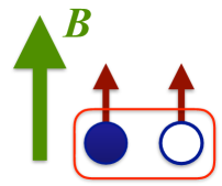
Condensates or the vacuum expectation values of physical operators should generally depend on external parameters such as the temperature, the density, and the electromagnetic background fields. It is thus an interesting question how changes when a finite is turned on as studied in a pioneering work of Ref. [21]. Intuitively, it is naturally anticipated that would favor a formation of the scalar condensate from the following argument. To assign proper quantum numbers to a composite state of a particle and an anti-particle, in the non-relativistic language, the scalar condensate must have the orbital angular momentum to cancel the intrinsic parity which is opposite for a particle and an anti-particle. Then, is required to make the total angular momentum . Even though the whole quantity, , is charge neutral and has no direct coupling to , from the microscopic level, we may well expect that such a spin-triplet configuration could be intrinsically more favored by , which is schematically illustrated in Fig. 1.
In most interested cases, , i.e., the scalar condensate as a function of magnetic strength should increase with increasing . Such increasing behavior is actually the case in the strong interaction physics in which the low-energy theorem holds including the magnetic effect [22], which was revisited more extensively in Ref. [23]. Although this tendency itself is rather robust not sensitive to specific theory, the precise dependence on should be different for different interactions and degrees of freedom contained in the theory. In the literature, this general tendency of increasing with increasing magnetic strength is commonly referred to as the magnetic catalysis.
In the original context [18, 24], however, the magnetic catalysis is defined in a more strict manner. It has been found that the magnetic field plays a role as a catalyst to cause nonzero for even infinitesimal interaction coupling. The statement shall be:
| Magnetic Catalysis: The scalar condensate takes a nonzero expectation value for even infinitesimal attractive coupling if the system is placed under sufficiently strong magnetic field. |
Roughly speaking, it is caused by low-dimensional nature; the system under strong magnetic fields is effectively reduced to (1+1) dimensions. Then, the gap equation for exhibits the same structure as that for the gap energy in superconductivity for which the Fermi surface realizes one dimensionality. In fact, plugging Eq. (14) into Eq. (17), performing the four-momentum integration which yields to compensate for the mass dimension 4, we finally get,
| (18) |
where a ultraviolet cutoff is adopted and denotes the incomplete gamma function. To arrive at the last expression, the integration contour is rotated as and then is approximated to be unity for large , which corresponds to the LLLA. Because for small , we understand that should behave like for small . The operator is conjugate to , so that is obtained by the -derivative of the energy . Therefore, such behavior of means that should contain a term . This observation will be soon verified in the subsection where we will see a model calculation of as a function of and the coupling constant .
2.2.1 Direct calculation
My goal in this subsection is to present direct calculations employing an interacting model. The model is defined with the following Lagrangian density:
| (19) |
for which the bare mass is assumed to be vanishing, , and is the coupling at the ultraviolet scale . This type of model is commonly called the Nambu–Jona-Lasinio (NJL) model [20] (for extensive reviews on the NJL model, see Refs. [25, 26]), which is a relativistic extension of the BCS model.
In the mean-field approximation, a quantum field is decomposed as , with which higher-order fluctuations in are neglected. In this approximation the mean-field Lagrangian density reads:
| (20) |
Now we understand that gives rise to an effective mass term, namely, . To determine the energetically favored value of , we need to evaluate the energy as a function of , that is given in the mean-field approximation by
| (21) |
where is the ultraviolet cutoff scale. The first term represents the zero-point oscillation energy, and the second is the condensation energy from the mean field. Introducing a dimensionless variable, , the energy can be expanded as
| (22) |
The trivial vacuum at becomes unstable when the quadratic coefficient in front of is negative. There are two competing effects for this coefficient; the zero-point oscillation energy always has a negative coefficient favoring a nonzero , while the condensation contribution has the opposite sign. Therefore, if the coupling is large enough, the condensation energy is suppressed, and the zero-point oscillation energy overcomes to lead to a finite or . Thus, the spontaneous generation of dynamical mass requires a large enough , i.e.,
| (23) |
We need higher-order terms to locate an optimal value of . The above calculations are relatively simple, and yet, surprisingly, this successfully accounts for the origin of masses.
Let us repeat the same procedure for the system with strong magnetic field. For simplicity the magnetic field is assumed to be strong enough to justify the LLLA in which the phase space integration is replaced by the Landau degeneracy factor and the (1+1)-dimensional integration:
| (24) |
We note that there is only one spin degrees of freedom in the LLLA as a result of the projection by , and so the overall spin factor 2 does not appear in the right-hand side in the LLLA above. Then, we can compute the energy as
| (25) |
This form of the expanded energy is extremely interesting. As we promised, a term appears. Thus, the quadratic coefficient is or dependent, and for , the coefficient involving becomes arbitrarily large, which means that the negative coefficient can always overcome to make unstable for even infinitesimal coupling . Therefore, some is energetically favored as long as and are non-vanishing, and the condition (23) in this case is changed to . From the above expression of , interestingly, we can find an energy minimum even without term. Some calculational steps eventually reach,
| (26) |
The analogy to superconductivity is evident in view of the above expression. The dependence enters the gap as an essential singularity around , which is common to the BCS gap energy. In this way, at the same time, we see that particle masses are not physical constants but they exhibit “medium” dependence influenced by external magnetic fields.
2.2.2 Renormalization group analysis
It would be quite instructive to consider an alternative approach to understand the magnetic catalysis based on the renormalization group (RG) equation following discussions in Refs. [27, 28]. This RG criterion is a very powerful technique, and even when it is difficult to solve the gap equation in the broken phase, we can make an educated guess about the parametric dependence of the gap. This method is generally known as the Thouless criterion.
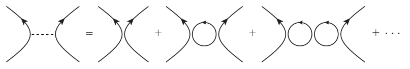
The point is that the four fermionic coupling is running with scale in the RG language; is the coupling after modes over are integrated out. The bare coupling in the Lagrangian density takes the ultraviolet value, at the scale , and should receive loop corrections sketched in Fig. 2 as goes smaller.
From a one-loop diagram we can find the function for as
| (27) |
We can directly solve this differential equation with the initial condition of at , leading to
| (28) |
which increases as goes smaller. If the above is expanded in terms of , the geometric series indeed correspond to loop corrections in Fig. 2. In the infrared limit, , the denominator is . Hence, diverges at some point of before reaching if
| (29) |
The divergent coupling implies that the scattering amplitude of a particle and an anti-particle has a singularity which signifies a formation of the bound state, like a formation of the Cooper pair in superconductivity. The above inequality is thus interpreted as the condition (23) in the mean-field approximation. The discrepancy by a factor 3 supposedly comes from different cutoff schemes.
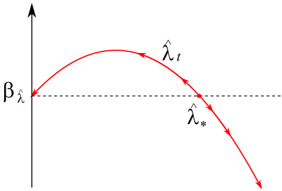
There is a more appealing way to understand the critical value of the coupling strength using the dimensionless coupling, . This rescaling to make dimensionless corresponds to the rescaling procedure in the conventional RG (Kadanoff) transformation. Then, the function for the rescaled coupling is translated into
| (30) |
where the first term is added from the mass dimensionality of the coupling . Then, the zero of the function is located at . If the RG running is initiated from , then is positive, and so becomes smaller as gets smaller, which is schematically illustrated in the left panel of Fig. 3. On the other hand, if the running is launched from , then is negative and keeps increasing with decreasing and it eventually diverges as shown in the left panel of Fig. 3. In this way, from graphical analysis, we can identify the critical coupling in Eq. (29) from the zero of without solving the differential equation.
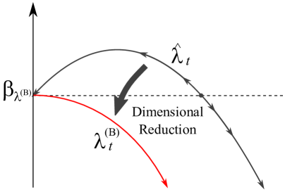
Now that we established our understanding without magnetic field, let us apply this argument to matter under strong magnetic field. We adopt the LLLA and replace the transverse phase space integration by the Landau degeneracy factor, which modifies Eq. (27) into
| (31) |
which can be directly solved as
| (32) |
Here, ranges from (at ) to (at ), and so the denominator can become zero for sufficiently large negative if only . This is precisely what is expected from the magnetic catalysis. As we did for , we can define dimensionless coupling, . In this case associated is as simple as
| (33) |
for which the zero is found only at . This drastic difference from Eq. (30) is attributed to the transverse phase space. For Eq. (30), by definition, the dimensionless coupling contains running with , but for Eq. (33) the magnetic field is a more relevant scale. Then, running is lost due to the dimensional reduction from (3+1)- to (1+1)-dimensional dynamics. We see that in Eq. (33) is entirely negative, which means that inevitably diverges for any initial . That is, the magnetic catalysis is again concluded from the dimensional reduction.
2.3 Inverse Magnetic Catalysis
The magnetic field has a general tendency to favor the scalar condensate, as we have discussed, but sometimes the resulting effect appears opposite. Such an exceptional situation, i.e., decreasing behavior of the scalar condensate for increasing magnetic field, is called the inverse magnetic catalysis, and the first example was found in a system at finite density [29]. If the density is high enough, in fact, it is always the case that the scalar condensate does not increase but decreases with increasing magnetic field [30], which is universally confirmed also in the RG analysis [28].
Nowadays, the inverse magnetic catalysis refers to a different realization, namely, a situation of finite temperature environment in quantum chromodynamics [31], which is a non-Abelian Yang-Mills theory with several flavors of fermions. This version of the inverse magnetic catalysis at finite temperature depends on microscopic dynamics of theory and there is no simple way to explain underlying mechanism. Nevertheless, since the recognition of the inverse magnetic catalysis posed lots of theoretical problems in the field of high-energy nuclear physics, we will go through to make some remarks on the finite-temperature phase transitions.
In short, the inverse magnetic catalysis can be defined as
| Inverse Magnetic Catalysis: The scalar condensate is decreased if the external magnetic field is applied to the system and its strength is increased. This may happen due to interplay with other external parameters and/or other dynamics of the theory affected by the magnetic field. |
2.3.1 Finite density
The scalar condensate is suppressed at finite density or finite chemical potential . We shall consider the effect of finite density using the NJL model again. At finite density the energy function, Eq. (21), is slightly modified as
| (34) |
One may notice that, if is larger than , there is no dependence at all, and this should be of course so. As long as is small not exceeding the mass threshold, no finite-density excitation is allowed, and thus no density effect should be visible. In what follows below we assume , and then we can relax the modulus in the above energy expression, simplifying it into
| (35) |
where . We can easily make sure that the finite- correction by the first term produces a term, , at the quadratic order in , which energetically favors . When a magnetic field is imposed, the density of states is changed; continuous excited levels become shrunk into the discrete Landau levels with degeneracy. Therefore, this finite- term to favor is enhanced at larger magnetic field since the density of states is squeezed by the magnetic effect. In summary, in this case of finite density, the inverse magnetic catalysis occurs as a result of finite- effect enhanced by the magnetic field. There is no theoretical difficulty; the inverse magnetic catalysis is to be observed already in the mean-field approximation.
2.3.2 Finite temperature
The NJL model is a relativistic cousin of the BCS theory. In this type of the theory the critical temperature, , is proportional to the gap, , at zero temperature, i.e., , where is defined by the condition, . Because the magnetic catalysis with larger drives to a larger value, finite- calculations using the NJL model predict that the melting temperature, , where is reached, monotonically increases with increasing .
In the context of the strong interaction with quarks and gluons, such a possibility to shift of the system exposed to strong has attracted a lot of theoretical interest. Quarks and gluons interact nonperturbatively, and it is believed that the color charge is confined and the effective mass is dynamically generated in the low temperature phase. At high temperature the coupling constant runs with the energy scale and the system enters a weak-coupling regime, where both color confinement and dynamical mass generation are lost. Because these phenomena are clearly distinct, there is no necessity for two temperatures of deconfinement and melting to coincide. Numerical simulations in the first-principles theory of the strong interaction have revealed, however, that two phenomena occur almost simultaneously at one critical temperature.
This observation of the common critical temperature strongly suggests that the origins of confinement and dynamical mass generation are not distinct but should be traced back to some common microscopic mechanism in the first-principles theory. As an attempt to model a locking mechanism underlying confinement and mass generation, the NJL model has been augmented to what is called the PNJL model [32, 33] including not only but also another order parameter corresponding to confinement. The PNJL model in a strong magnetic field predicted disentanglement of two phenomena; is affected by the magnetic catalysis, while confinement belongs to the dynamics of gluons which are electric charge neutral, and thus the deconfinement temperature is hardly changed by the magnetic effect. If this is the case, the phase diagram of strongly interacting matter out of quarks and gluons would open a new window in which confinement is lost but fermions are still massive [34, 35].
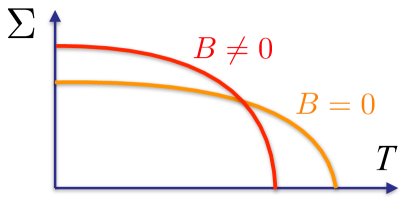
With this background stories in mind, one may imagine how much surprised people were at numerical results from the first-principles simulation claiming that there is no disentanglement but the common phase transition temperature is lowered by a stronger magnetic field [31, 36, 37]. This means, if the order parameter is plotted as a function of for zero and nonzero magnetic field, gets larger at small , but drops steeper with increasing , as illustrated in Fig. 4.
It is nearly impossible to explain such an exotic pattern of modifications on from the dynamics of mass generation alone (see Ref. [19] for a scenario closed in the chiral sector), and the coupling to confinement sector incorporated in the PNJL model is still insufficient to realize this pattern. In other words, the finite- inverse magnetic catalysis is a serious challenge to such model studies. Clearly the PNJL model must miss something in the confinement or gluonic sector. In fact it has been known from applications to high-density matter that the gluonic potential used in the PNJL model lacks backreaction from quark polarizations on gluon propagation (for the LLLA estimate for the polarization effect, see Ref. [38] and for the full Landau level calculation, see Refs. [39, 40]). For another nonperturbative backreaction, see Ref. [41]. These missed diagrams make the strong coupling run with energy [42], as runs with in the previous subsection. The asymptotic freedom implies that is a decreasing function of and both. Some theoretical calculations demonstrated that there may be a window in which has a local minimum as a function of , which explains the inverse magnetic catalysis [43].
Interestingly, in the vicinity of deconfinement transition, duality between deconfined quark and confined hadronic degrees of freedom could hold. Therefore, the inverse magnetic catalysis may be approached from the hadronic side. In the hadronic phase there are many composite states of quarks which carry electric charge such as the charged pions and the proton. Such charged hadrons with nonzero spin become lighter significantly as a result of the Zeeman coupling with the magnetic field. In this way, as an extension from Ref. [44], it has been numerically confirmed that the “critical” temperature inferred from rapid changes in thermodynamic quantities is shifted down toward a smaller value for strong magnetic field [45]. This is a dual picture to view the inverse magnetic catalysis.
2.4 Toward more realistic descriptions
We have idealized the physical setup assuming infinite volume and spatial homogeneity, but in reality, the system size, that is the size of matter distribution and/or applied magnetic field, is finite. When we discuss rotation effects later, it will be crucial to take the finite size seriously; otherwise, the causality is violated. One may think that such finite size effects are anyway small corrections, but as we will see here, qualitatively new physics is perceived from those analyses.
2.4.1 Solvable example of inhomogeneous magnetic field
It is generally a hard task to solve quantum field theory problems without translational invariance. Inhomogeneous electromagnetic backgrounds break translational invariance, and there is no universal algorithm to take account of such fields. Thus, if any, some theoretical exercises using analytically solvable examples would be helpful for us to sharpen our feeling about the effect of inhomogeneous fields.
One well-known solvable example is the Sauter-type potential. The Sauter potential literally means a time-dependent electric potential, which was studied as an attempt to resolve the Klein paradox [46], which we will discuss later in Sec. 3. Here, with a magnetic counterpart of the Sauter-type potential, the magnetic field is directed along the -axis and the spatial dependence is one-dimensional along the -axis like
| (36) |
This magnetic distribution is peaked around and the wave number characterizes the typical scale of the spatial modulation. The Sauter-type magnetic configuration can be described by the following vector potential:
| (37) |
which smoothly reduces to in the limit of .
The eigenvalue spectrum and the wave-functions can be found in Ref. [47] (in which the potential is called the modified Pöschl-Teller form) for both fermions and bosons. We will not repeat the derivation here but jump to the final results for fermions. The energy dispersion relation for Dirac particles under of Eq. (36) is, , where, for integer (which also defines the range of to keep ) and , the eigenvalue is given as
| (38) |
This expression can become much simpler for small inhomogeneity if only is satisfied, and then we can remove the modulus to simplify the above expression for as
| (39) |
with and , which also constrains the possible range of . We can immediately convince ourselves that the ordinary Landau quantization is recovered for . Then, for and correspond to the spin up and down Landau levels. In particular the Landau zero mode, , exists for one spin state only. In this case of the -integration yields the Landau degeneracy factor which is regularized by the system size. In other words the Landau degeneracy factor is proportional to the magnetic flux which would diverge for infinitely large systems.
The eigenvalue spectrum of Eq. (39) is very useful for us to develop our intuition about the effect of inhomogeneity. The most notable feature is that, interestingly, even though the magnetic field is inhomogeneous, the Landau zero mode, , exists (but the degeneracy factor could be modified). This observation could be a manifestation of the Atiyah-Singer index theorem; see Ref. [48] for more discussions. Moreover, the higher excited states are pushed down overall by inhomogeneity. Let us go a little more into concrete numbers for the low-lying states.
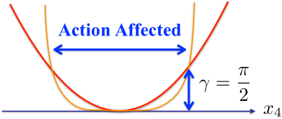
For homogeneous magnetic field with , the first Landau level is located at with spin degeneracy. The degeneracy with respect to is lost by . Here we shall assume and expand the eigen-energies in terms of . We then approximately obtain up to the order. Therefore, the LLLA might be suspicious if is comparable to interested energy scale even though itself is sufficiently large, which is quite natural because the magnetic field is then damped quickly. In the same way, the second Landau level is perturbed to spread over , and so the minimal energy gap is again of order not but . Therefore, inhomogeneous magnetic fields soften one-particle excitation energies. If , one can also perform diagrammatic perturbative expansion, as done in Ref. [49], to get some confidence about the generality of the above statement.
Now we should be cautious about the lower bounds in the limit. Seemingly all lower bounds of spreading spectrum approach zero (i.e. , , etc) as goes smaller, and if so, the discrete spectrum at cannot be retrieved smoothly from the limit. In drawing Fig. 5 we assumed that can be as large as , but in reality, is cut off by a combination of the magnetic field and the system size. Then, with bounded smaller than in such a way, the spectrum shrinks to the discrete one in the limit as it should.
2.4.2 Finite size and surface effect
Instead of considering inhomogeneity in the applied magnetic field, we will turn to a different but somehow related problem in this subsection, that is, the finite size effect. We do not want to break translational invariance along the magnetic direction (i.e., the -axis), so the simplest geometrical setup is given by the cylindrical coordinates, . Before considering the boundary effect on magnetic systems, let us first take a close look at the solutions of the free Dirac equation for in the cylindrical coordinates. For particles with positive energy, two helicity states can be written down explicitly as
| (40) |
where the onshell condition is . We see that these are simple generalization from the standard expression (6) with for . There are, however, two major differences from Eq. (6). One is that the transverse coordinates, and are replaced by and whose conjugate momenta are, respectively, and . The other is that is discretized by the system size or the cylinder radius . That is, no flux condition at leads to the discretized momenta as
| (41) |
where is the -th zero of the Bessel function . We can immediately write down the anti-particle solutions using the -parity transformation, i.e., as
| (42) |
Again, it is clear that these are generalizations from Eq. (6) with appropriate choice of . We also note that have the angular momentum and have along the -axis.
Now, next, it is time to activate finite magnetic field. The positive-energy particle states with the -component of the angular momentum, , are only slightly modified as [50]
| (43) |
in which the Bessel function is upgraded to a more general special function. With the confluent hypergeometric function (Kummer’s function of first kind), this upgraded functions are defined as
| (44) | ||||
| (45) |
The discretization condition for the transverse momenta is also changed as and
| (46) |
where is -th zero of with . We note that is nothing but the Landau degeneracy factor, . It would be more understandable if we see Eq. (46), not as a finite- generalization of Eq. (41), but as a finite- generalization of the standard Landau levels. In fact, if or is sufficiently large, has -th zero at for nonnegative integer .
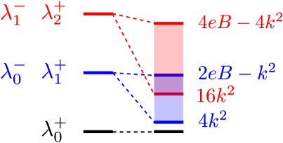
Figure 6 shows as a function of for various . For zero magnetic field (i.e., ), the symmetry under is manifest. In our convention is the component of the total angular momentum, and corresponds to . Such symmetry of sign flip of the total angular momentum is explicitly broken by the Zeeman energy from the orbital-magnetic and spin-magnetic coupling. We actually know that the Landau zero mode has only one spin state; as seen in Fig. 6, for finite , nearly zero degenerate states of spread only in the positive- side. If is strong enough and/or is large enough, the boundary effects should be negligible and the Landau degeneracy of should approach . In Fig. 6, for for example, the flat bottom region ends around , and so is not yet large enough to enter the regime of the full Landau degeneracy .
One might think that the anti-particles could be constructed by as we did previously, but this transformation does not work. In the presence of external magnetic field or vector potential in general, the -parity symmetry is explicitly broken (noting that the vector potentials are -odd), so does not satisfy the Dirac equation. The direct calculations result in
| (47) |
We note that in Ref. [50] the anti-particle solutions are given with changed to , which means that the above states have the angular momentum , while such anti-particle states in Ref. [50] have . The convention of Ref. [50] is practically useful, but the spin quantum number in the above expression is more in accord to our intuition. In the present choice the approximate Landau zero modes of appear for negative- region since above involve . Therefore, the angular momenta of those nearly Landau zero modes should be positive. In this way, we observe a peculiar pattern in the Landau zero modes that, for particles and anti-particles, the favored spin alignments are opposite and yet the total angular momenta are degenerated. This corresponds to the fact that the magnetic responses of particles and anti-particles should be opposite, but if a small rotation is introduced perturbatively, the rotational effect would not discriminate particles and anti-particles.
Now that a complete set of wave-functions comes by, we can compute the propagator and any operator expectation values perturbatively. In fact, in Ref. [50], the scalar condensate has been calculated in the local density approximation. Then, it has been found that the magnetic catalysis is significantly strengthened near the boundary surface, , due to the accumulation of large- wave-functions. Anomalous contributions near the surface may play a crucial role to fulfill global conservation of some physical charges.
Summarizing the discussions in this subsection, we constructed explicit solutions of the Dirac equation with a boundary condition at . The finiteness of the system is important for phenomenological applications; the Landau degeneracy factor diverges for infinite sized systems, and such a simple estimate, , based on homogeneous treatment is not necessarily a good approximation. Moreover, the identification of anti-particles is nontrivial. It was not my intention to bother readers with technical details, but above expressions are firm bases to visualize the physics.
3 Dynamical Problems with Electromagnetic Fields
We will explore some formalisms to cope with not only the magnetic field but also the electric field. We will start with a case with only the electric field to study the Schwinger Mechanism, and then turn on a constant magnetic field. The coexistence of the parallel electromagnetic fields would break the - and -symmetries, and such an electromagnetic configuration is a theoretically idealized setup to probe the chiral anomaly. We will introduce an idea called the chiral magnetic effect (CME) as a clear signature for the chiral anomaly.
3.1 Schwinger Mechanism
Quantum field theory calculus was completed in Ref. [51] and the generating functional, which is an amplitude from the past vacuum to the future vacuum, was found to acquire an imaginary part in the presence of constant electric field. The appearance of imaginary part generally signifies a kind of instability. There have been some confusions about the theoretical interpretation about the imaginary part (see Ref. [52] for judicious discussions on this issue). For some historical backgrounds together with the treatment of the Sauter-type potential, see also Ref. [5]. A comprehensive review on the Schwinger Mechanism including latest developments can be found in Ref. [6]. For beginners a textbook [53] is also recommendable. In the present review I would not touch such a subtle argument, but I would rather prefer to formulate the same physics in terms of the particle production amplitude [54].
The particle production can occur whenever the energy-momentum conservation is satisfied and the quantum numbers are matched. In the case of the pair production, the momentum conservation can be satisfied if only the emitted particle and anti-particle are back-to-back placed. Because such particle and anti-particle carry finite energy, the external fields should inject an energy into the system. It is obviously impossible to balance the energy with homogeneous magnetic field only which gives no work on charge particles. If a pulse-like electromagnetic field externally disturbs the system, a virtual (offshell) photon from the electric field can decay into a pair of a particle and an anti-particle, and in this case, a vertex of photon, particle, and anti-particle gives a tree-level contribution to the pair production amplitude. Thus, nothing in particular is special in the pair production process with pulse-like fields.
A surprise comes from the fact that even a constant electric field can supply a finite energy, which allows for the pair production. As we will discuss later, the introduction of constant electric field assumes a time-dependent background vector potential. The time-dependence is, however, infinitesimal, and thus, the energy transfer from a perturbative process with this background field is infinitesimal. Therefore, a single scattering cannot meet the energy conservation law, but then, what about multiple scatterings? Even if the energy transfer from each scattering is infinitesimal, infinitely many scatterings eventually amount to a finite energy so that the energy conservation can be satisfied. This nonperturbative process for the pair production driven by constant electric field is called the Schwinger Mechanism, i.e.,
| Schwinger Mechanism: The vacuum under constant electric field is unstable to produce pairs of a particle and an anti-particle via nonperturbative processes. |
It is often said that the Schwinger Mechanism is a result of quantum tunneling. Actually, we can formulate a pair production as a conversion process from an anti-particle (negative-energy state) in the Dirac sea to a particle (positive-energy state). The particle and the anti-particle states are gapped by the particle mass, , which may well be regarded as a sort of activation energy, and then the electric field is like the temperature. In this way there have been some theoretical speculations about a possible connection between the Schwinger Mechanism and thermal nature of produced particles. In fact, as we will elaborate below, the tunneling amplitude is characterized by the Bogoliubov coefficient in a way very similar to the Hawking radiation process from the blackhole (see Ref. [55] for detailed derivation of the radiated spectrum). There is a significant difference, however, in the final expressions; the rate in the Schwinger Mechanism is exponentially suppressed like which is much smaller than the Boltzmann factor for large .
3.1.1 Solvable example of time-dependent electric fields
Here, I would not intend to explain mathematical techniques to solve the differential equation, but using a solvable example I would present a demonstration to concretize some important concepts on the Schwinger Mechanism. The solvable example, i.e., the Sauter-type electric profile is
| (48) |
which is realized by the following vector potential,
| (49) |
This example was found by Sauter in 1932 [46] to discuss the Klein paradox, that is a puzzle of inevitable transmission of fermions over electric barriers. As a matter of fact, the Schwinger Mechanism is a field-theoretical solution to the Klein paradox. Coming back to the calculation, we notice that in Eq. (49) takes different values in the in-state at and the out-state at , while in Eq. (48) goes to zero at both , as displayed in Fig. 7. The background gauge potential shifts the energy dispersion relations of the in- and the out-states, respectively, as
| (50) |
where is defined.

We can quantify the particle production by computing the Bogoliubov coefficients, that is, coefficients connecting the creation/annihilation operators in the in- and the out-states. For this purpose, we can solve the equation of motion from the initial condition of either a particle state or an anti-particle state, that is,
| (51) |
which evolves into
| (52) |
If no electric effect is applied, there is no mixing between particles and anti-particles and thus and trivially. A nonzero represents the tunneling amplitude from the anti-particle to the particle (and vice versa). With these coefficients for fields, taking account of the field expression in terms of creation/annihilation operators, we can identify the Bogoliubov coefficients as
| (53) |
The produced particle distribution, , which is defined by the number operator expectation value as , is given by
| (54) |
For the Sauter-type potential the solution is known and the Bogoliubov coefficient reads [56]:
| (55) |
where and . This distribution function is plotted for [where ] as a function of in Fig. 8.
From Fig. 8 we see that the pair production rate is peaked at for which the above expression becomes much simpler with and thus . At this peak position, we can take limit to consider constant electric field, to find that the above expression reduces to
| (56) |
This exponential factor is typical for the Schwinger Mechanism. The transverse momentum integration gives a prefactor by the phase space . The remaining exponential characterizes the critical value, sometimes called the Schwinger critical electric field, whose expression is
| (57) |
I must emphasize that nothing is truly critical at this critical electric field. There is no phase transition nor avalanche phenomenon but the above relation is just an order estimate for the electric field necessary for a sizable amount of pair production.
3.1.2 Worldline instanton approximation
Now we would like to turn on a magnetic field on top of electric field. If these fields are constant, such a problem is solvable, though the technical details are quite complicated (see Ref. [5]). Here, we shall take a bypass, i.e., instead of getting a rigorous answer, we make less efforts and approximate formulas correctly on the qualitative level. We further assume in this section. In later discussions we will be interested in the chiral anomaly, which is detectable with background .
In this review I will entirely neglect backreaction from gauge fluctuations (see Ref. [57] for simulations with backreaction), but focus on the response of matter under fixed gauge background. Thus, it is sufficient to consider a fermionic part of the action. Because fermions enter gauge theories in a quadratic form unlike the NJL model where four fermionic interactions are assumed, we can simply identify the Dirac determinant as the full effective action, that is,
| (58) |
where the covariant derivative is . From the middle to the right expression we multiplied which duplicates the Dirac determinant. We note that this trick is useful as long as the -Hermiticity holds; for example, a finite chemical potential breaks this property. The last term involving the spin tensor, , represents the spin-magnetic coupling.
It is straightforward to reexpress in terms of the proper-time integration, as we saw in Eq. (12), using a general operator relation,
| (59) |
Here, is to be replaced by the Dirac operator, and is then regarded as time evolution by a “Hamiltonian”, , with an “imaginary-time” , which can be viewed as a quantum mechanical system evolving from at to the same at due to the trace nature. We can adopt Feynman’s path integral representation to describe this quantum mechanical evolution for . For step-by-step transformations in detail, see Ref. [58]. After all, the derivatives or the momentum variables in the Hamiltonian are translated into in the Lagrangian system as
| (60) |
where represents the integration under the periodic boundary condition; . It should be mentioned that the above expression assumes the Wick rotation to Euclidean variables, . The last part, , corresponds to the matrix part in Eq. (58). For our special problem with and , this last part can become factorized into the electric and the magnetic contributions as
| (61) |
Therefore, the fermionic effective action takes the following semi-factorized form:
| (62) |
Here, introducing a dimensionless variable , we can write down the explicit forms of the electric and the magnetic terms as
| (63) | ||||
| (64) |
where represents the -derivative of . Interestingly, for constant electromagnetic fields, these kernels can be evaluated without approximation, that is,
| (65) |
Then, the effective action can be expressed without approximation as
| (66) |
This proper-time integration could be directly performed, which is dominated by pole contributions around where is singular. This singularity structure implies that must have a series expansion like with some coefficients of order unity.
An exact solution is of course useful, but I would rather prefer a more adaptive method applicable to a wide variety of physics problems. The worldline instanton approximation is such a flexible strategy and at the same time some interesting physical interpretation is possible. To see this, let us go back to the expression of in terms of and . Then, before performing the and integrations, we shall first treat the -integration. There are two completing dependence on the exponential; one is from the mass, , which favors smaller , and the other is from the electric kinetic term, , which favors larger . One might have thought that the magnetic sector has a similar term, but we already know the answer after the integration, which behaves like for large , and has no effect on the location of the saddle point.
We follow the physics arguments in Ref. [59]. We can find the saddle-point to approximate the -integration at
| (67) |
Then, the effective action is approximated as
| (68) |
where we can easily get on the exponential from this expression of , that is,
| (69) |
We should then take care of the and integrations. If is large, which is normally the case for the Schwinger problem, we can utilize a semi-classical approximation, i.e., the and integrations should be dominated by classical trajectories which (locally) minimize . The minimization condition is nothing but the equation of motion, and the solutions of the equation of motion are commonly referred to as “worldline instantons” for the reason explained later. It is very easy to take a variation on to find the equation of motion as
| (70) |
for . A proper combination of these equations immediately proves , which simplifies the denominator in the left-hand side of the equation of motion. Plugging (where is the Euclidean field strength and is the Minkowskian physical electric field), imposing the periodic boundary condition , and choosing the initial condition , we can obtain the solutions of the equation of motion:
| (71) |
characterized by . These are very interesting solutions; in Euclidean spacetime implies in Minkowskian spacetime making hyperbolic trajectories, which are solutions under an acceleration. With these solutions, we see that the saddle point of is located at , which coincides with the singularities in . Thus, we arrive at the same conclusion of the integration dominated around though we exchanged the order of the integrations; first and later or vice versa. The action with these solutions becomes:
| (72) |
The prefactor in the saddle point approximation can be also calculated, and then we eventually reach the single pair () production rate (i.e., pair numbers per unit volume and time) inferred from . Such an expression for the particle production rate in the presence of parallel electromagnetic fields will be, in the next subsection, the key equation for our analysis on the chiral anomaly. What we learnt here is summarized as follows:
| Schwinger Pair Production Rate: The rate of single pair production in the presence of paralle electric and magnetic fields is given by the formula: (73) |
One notable advantage in this method of the worldline instanton approximation is the generality which can be directly applied to a case with time-dependent electric perturbation. A very interesting idea has been proposed in Ref. [59]; the Sauter-type potential is weakly perturbed from Eq. (48) as follows:
| (74) |
where . The corresponding vector potential in terms of Euclidean time , up to irrelevant constants, reads:
| (75) |
In the worldline instanton approximation, we can make use of our knowledge on classical mechanics. Even without solving the equation of motion, in classical mechanics, the energy conservation law easily derived from the equation of motion can give us an intuitive picture about the motion. In fact, the equation of motion (70) leads to the conservation law for the sum of the kinetic and the potential energies as
| (76) |
For sufficiently small , the first term in is well approximated by describing a homogeneous electric field. The second term, is infinitesimal for small except when approaches where diverges. Therefore, in this case, is an energy potential given by a superposition of a quadratic term and infinite energy barriers at as sketched in Fig. 9. Therefore, nothing changes from the previous case without time-dependent perturbation unless the solution of the equation of motion reaches . In other words, the motion is restricted from to (where ) defined by above the threshold. The critical condition for this threshold is, , that is, . It is extremely interesting that the action is modified even though the magnitude of the time-dependent perturbation is arbitrarily small. Actually, the exponential factor, appearing in the pair production formula, is suppressed above the threshold as [59]
| (77) |
and this reduced exponent is characteristic to what is called the dynamically assisted Schwinger Mechanism. For consistency check, at the threshold , we note that the above expression recovers the familiar Schwinger result, .
3.2 Chiral Anomaly and Axial Ward Identity
In this subsection we will address an application of the Schwinger Mechanism to investigate the chiral anomaly. If the fermion mass is zero in the Dirac Lagrangian density, the axial vector current should be a conserved Nöther current on the classical level. With quantum corrections, however, the conservation law of the axial vector current is not compatible with the gauge invariance. Because the gauge symmetry must not be broken (otherwise, the renormalizability is damaged), the axial vector conservation should receive a correction which breaks down the classical conservation law. For given gauge background the violation of the conservation law is precisely quantified in a way known as the axial Ward identity:
| Axial Ward Identity: The divergece of the axial vector current is zero if all the fermion masses are zero on the classical level, which is modified by quantum corrections. If the theory has one Dirac fermion and Abelian gauge background fields, the violation is formulated on the level of the operator identity as (78) |
In the presence of parallel and , therefore, the expectation values taken on the axial Ward identity read:
| (79) |
where we used (which can be checked by explicit calculations). This expression has an interesting interpretation. Let us assume that we can drop the last term in the chiral limit of (whose validity is far from trivial as we will argue later). Then, we can derive the above relation from a very classical consideration.
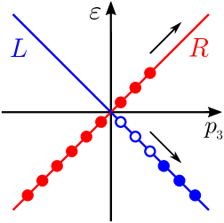
For sufficiently strong background of , the dimensional reduction occurs and the (1+1)-dimensional fermionic dispersion relations belong to the right-handed and the left-handed helicities as shown in Fig. 10, which is essentially the same figure found in Ref. [60]. The Fermi momentum of the right-handed particles increases with and its phase space volume gives the increasing rate of the right-handed number density, , as
| (80) |
in reduced (1+1)-dimensional dynamics. For the left-handed particles the number density decreases, whose rate is given by the above expression with the opposite sign. The physical interpretation of Fig. 10 is transparent; under strong together with the pair creation produces a right-handed particle and a left-handed anti-particle, incrementing the chirality by two. Then, the total particle number is conserved, but the chirality density, , changes in (3+1) dimensions as
| (81) |
multiplied by the transverse phase space by the Landau degeneracy factor, . This result perfectly agrees with Eq. (79) if is .
More importantly, the above mentioned derivation of the chiral anomaly based on the pair production of a right-handed particle and a left-handed anti-particle leads to a quite suggestive relation, that is,
| (82) |
where represents the Schwinger pair production rate (73).
3.2.1 In- and out-states
If the particle mass is zero, i.e., , it seems that Eq. (82) appears consistent with Eq. (73). This statement is what is frequently said in the literature, but we will see that the fact is far more complicated. To this end, we need to evaluate .
It was Schwinger [16] who first calculated using his proper-time integration technique. In the vacuum such a pseudo-scalar condensate is vanishing, but with being -odd and -odd, a finite expectation value should be induced as . Then, the direct calculation results in
| (83) |
for constant and parallel electromagnetic field without approximation. By substituting this for the axial Ward identity, we have to conclude that
| (84) |
for any including the limit. This result is astonishing, though this is correct! First, Eq. (84) obviously contradicts an expected relation (82). Second, the last term in Eq. (78) can not always be dropped in the chiral limit of . Because the condensate behaves like , the -dependence in the term cancels out with the condensate and such a combination may survive. Third, the right-hand side of the axial Ward identity is zero, so that the axial vector current can be conserved. There is no way to access the chiral anomaly which existed on the operator level but disappears as an expectation value.
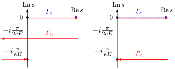
We can resolve this apparent puzzle once we notice that there are inequivalent ways to take the expectation values in the presence of electric field. That is, as we already learnt from Fig. 7, an electric field causes a difference between the in-state, , and the out-state, , which makes them distinct states. In the standard calculus of Schwinger’s proper-time integration, the expectation value generally calculable in Euclidean theory corresponds to . Strictly speaking, this expectation value is not a physical observable, but an amplitude whose squared quantity is given an interpretation as a physical observable. To put it another way, is just an expectation value in Euclidean theory which is naturally realized in the limit of finite-temperature quantum field theory. So, we may say that is a static or spatial expectation value. We thus need to cope with in order to access the dynamical or temporal properties of the problem.
In Ref. [62] it has been pointed out that a textbook [61] developed convenient technologies for the treatments of and . The conventional Schwinger proper-time integration goes on as depicted in Fig. 11, which yields . For of our current interest, we should choose the deformed contours, for and for . Therefore, the induced pseudo-scalar condensate has the following representation:
| (85) |
where is either or ; because the integrand contains no singularity, both give a unique answer. The above answer is consistent with the discussions also in Ref. [63] in which quantities have been addressed for the field-theoretical computation of , that is the left-hand side of Eq. (82). For the field-theoretical formulation of , see also Ref. [54]. Now, it is clear that Eq. (82) holds with Eq. (85) as it should.
3.2.2 Electromagnetic realization of the chiral magnetic effect
We have seen that the Schwinger Mechanism describes a physical process of pair production of a right-handed particle and a left-handed anti-particle if applied is strong enough. Apart from the backreaction, therefore, the pair production induces a chiral imbalance onto the system. It is known that such a chiral imbalance coupled with external magnetic field would be a source of exotic phenomenon in connection to the chiral anomaly.
Before the application of the Schwinger Mechanism, we shall make a flash overview of the chiral magnetic effect (CME), that is a topologically induced signature for the chiral anomaly. There are many derivations and arguments, but one of the clearest passages leading to the CME formula is the Maxwell-Chern-Simons theory (aka axion electrodynamics), that is defined by the Maxwell theory augmented with the topological term:
| (86) |
The second term involving the angle is the Chern-Simons term, and as long as is constant, this term would not modify the equation of motion because is a total derivative. If we assume spacetime dependent , however, some additional terms appear in the equation of motion and the modified Gauss and Ampère laws read [64]:
| (87) | |||
| (88) |
From this expression, we see that new terms arise in the place of which can be identified as new contributions to the current. One might think that such induced terms could be a fictitious current like Maxwell’s displacement current, , as questioned in Ref. [7]. To answer this question, we should consider how the charge conservation holds for a finite system; actually, charge density emerges in a perfectly consistent way with the current , which means that this new current is a genuine current unlike Maxwell’s displacement current. Changing the notation from to , we arrive at the standard CME formula [65] (for a pretty complete list of preceding works including Vilenkin [66] and Giovannini-Shaposhnikov [67], see Ref. [4]):
| Chiral Magnetic Effect: A nonzero chirality imbalance is induced by , which is coupled with external magnetic field, , leading to an electric current parallel to as (89) |
This is a formula for a single fermion contribution. If the theory has multiple species of fermions, the above current is multiplied by the fermionic degrees of freedom. Interestingly, the formula is insensitive to the fermion mass, and it is independent of the temperature, as should be so for the quantum anomaly.
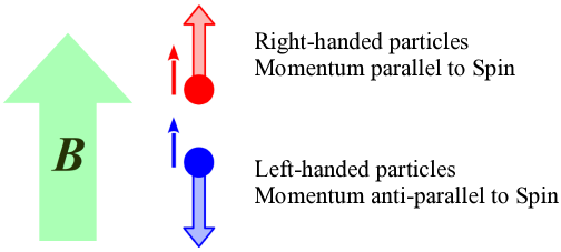
An intuitive view point to understand the CME is picturized in Fig. 12. By definition, the right-handed particles have the spin and the momentum in parallel directions, while the left-handed particles have anti-parallel spin and momentum. The spin direction is aligned along the magnetic field as shown in Fig. 12, which simultaneously fixes the momentum direction. A nonzero induces unbalanced chirality density, , and thus, a combination of and the spin-magnetic correlation generates a net current along the magnetic direction. Such an electric current is inherently anomalous that does not exist in classical electrodynamics in which the magnetic field does not transfer any work on charged particles. The energy is supplied by or in other words the driving force is provided by time-dependent .
Regarding the physical interpretation of the formula, there have been controversies. Some came from the derivation presented in Ref. [65]; the thermodynamic potential was calculated on background vector potential , magnetic field , and chiral chemical potential , and the current was estimated from . Nothing is wrong about this procedure, but strangely, this derivation implies the existence of the permanent current even in equilibrium! A state with current should be, even if it is time independent, a steady state out of equilibrium. In short, in equilibrium, the CME current must be prohibited by definition of equilibrium. Here, one must not be confused with the argument in Ref. [68], though the claim itself sounds similar. The important message from Ref. [68] is that the CME current does not exist in solid state systems where there is no Dirac sea (from which the anomaly arises) and also the surface term cancels out with periodic boundary condition (see also Ref. [69] for related discussions). In this sense, the statement of Ref. [68] is the same claim but made under tighter constraints, not applied to continuous quantum field theory. What I am emphasizing here is that even in continuous quantum field theory the CME current cannot be permitted in equilibrium.
A sort of consensus has been built in the community, that is, a nonzero is the trick to emulate a steady state using an equilibrium language. More concretely, should be zero in true equilibrium situation, and the introduction of nonzero forces the system to be out of equilibrium. Such an interpretation physically makes sense, but as long as is introduced by hand, there is no way to turn off effects to mimic off-equilibrium. One way to cure this situation is to take account of the relaxation process of decaying toward zero as the time goes.
Another (and more well-founded) theoretical approach would be to abandon using . The role played by is to inject an energy imbalance between the right-handed particle sector and the left-handed particle sector. We have already argued that the Schwinger Mechanism under strong magnetic field leads to exactly such chirality imbalance. Hence, we can just impose an external so that can replace . This idea was first proposed in Ref. [70] and analytical formulas based on the identification of Eq. (82) have been derived for a geometry of and making an angle less than (i.e., has both components and ). We have already seen that, surprisingly, the Euclidean expectation values make the right-hand side of the axial Ward identity vanishing, which also means that the CME current is vanishing then. Now, we have a better understanding of why this should be so; the CME current should be indeed vanishing for static systems described in Euclidean formulation, as was clarified recently in Ref. [62].
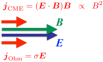
Later on, the simple idea of Ref. [70] was further simplified in Ref. [71]; no angle between and is necessary, but only the parallel is sufficient to probe the CME current as sketched in Fig. 13. The idea is the following. The minimal setup is just to impose an external magnetic field on chiral material along which a finite voltage is applied so that an electric current flows. Then, the electric field should be present there according to Ohm’s law, i.e., where denotes the Ohmic electric conductivity. Because of the electromagnetic background, a finite chirality is pumped up as as deduced from Eq. (73), which means that is anticipated. Then, the CME formula with implies the CME current, . From this relation we can deduce that the electric conductivity associated with the CME current has peculiar magnetic dependence . The experimentally observed current should be a superposition of , where is assumed to have only minor dependence on . Therefore, if an anomalous component of the electric conductivity increasing with or equivalently the electric resistivity decreasing with is confirmed, it would be a clear experimental signature for and thus the chiral anomaly. Such a behavior of the resistivity suppressed as is especially referred to as the “negative magnetoresistance” in the literature. Finally, let us make a remark on the asymptotic dependence in the strong- limit. In the above discussion a relaxation process of the produced chirality is implicitly assumed; otherwise, the chirality diverges over a long time. Actually in Ref. [71] the relaxation time approximation is adopted in the framework of the chiral kinetic theory, and also in Ref. [72] that is the very first report of the experimental observation of the negative magnetoresistance, a relaxation time is introduced in a Drude-type picture. Then, such quadratic dependence of the conductivity or resistivity is predicted if the relaxation time is independent. In reality, however, the relaxation time or the microscopic scattering process is significantly affected by -dependent phase space volume. A complete field-theoretical computation of the electric conductivity including higher Landau levels have revealed that the physical asymptotic dependence on is not quadratic but linear [73].
4 Phenomena induced by Rotation
In many physics problems the angular momentum causes a phenomenological consequence analogous to the magnetic effect. In fact rotating chiral matter would exhibit a current which looks similar to the CME current. This effect to generate rotation induced axial current is called the chiral vortical effect (CVE). Because the axial current operator is nothing but the spin operator in the relativistic language, the CVE could be regarded as a transport process from the mechanical rotation into the spin or the magnetization, which may well be a relativistic extension of the Barnett effect. Then, it would be a natural question to think of another relativistic extension, namely, the Einstein–de-Haas effect. These are new subjects and so we will only briefly look over speculative ideas.
Furthermore, recently, there are many interesting works to discuss the ground state properties affected by rotation effects, see Ref. [74] for a phase diagram, Ref. [75] for the scalar condensate, Ref. [76] for the pion condensation, etc. These are all exciting developments, but in this review, we will stay with simpler physics problems only.
4.1 Rotating Chiral Fermions
Rotation effect has been well understood in some fields of physics such as nuclear physics in which all deformed nuclei must rotate to restore broken symmetry in a finite system. Such a quantum system in a rotating frame can be described by the cranking Hamiltonian, that is, the Hamiltonian shifted by a cranking term, , where is the angular velocity vector and is the total angular momentum. Such an energy shift can be identified as an effective chemical potential. In this sense, a finite rotation has dual aspects as a magnetic counterpart and a finite-density counterpart. In particular the analogy between rotation and finite density has been pursued in Ref. [77] in which the rotation-induced inverse magnetic catalysis has been found. From this analogy the phase diagram as a function of the temperature vs. the rotation angular velocity can be considered, and similarity to the conventional phase diagram as a function of the temperature vs. the chemical potential has been verified in Ref. [74], with an importance exception. Suppose that the system is just rotated but no magnetic field nor temperature is introduced, then, the question is as follows; can a finite density be induced by the effective chemical potential by alone? The answer is negative. The finite size effect is crucial to make a correct statement. With discrete momenta, Eq. (41), the minimum energy gap is of order , and the effective chemical potential is also of order bounded by the causality, and one can prove that the former is always greater than the latter [78]. Therefore, only a finite rotation cannot change the ground state property, which is consistent with the equivalence principle.
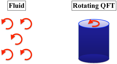
To incorporate rotational effect, two technically distinct treatments are commonly adopted; one method is a description with local vorticity vector of a fluid, and the other is with global rotation via coordinate transformation to a rotating frame, as schematically drawn in Fig. 14. Each has an advantage and a disadvantage. Because the vorticity is a local quantity, the former method has no necessity to be put in a finite sized system. Without the boundary, however, there is no simple way to take account of the orbital angular momentum (see Refs. [79] for examples of theoretical attempts for spinning hydrodynamics). The latter is in this sense more convenient in order to consider the orbital angular momentum of a finite system. Unlike the former fluid description, however, the center of rotation and the boundary at the surface make physical quantities inhomogeneous depending on the radial distance.
Here, I would stress that two treatments should be equivalent if the same physical system is considered. It is well known that, for example, a rotating superfluid forms a lattice of vortices which carry a quantized angular momentum, and as the rotating velocity of the superfluid increases, the number of vortices gets larger, and the integrated vorticity eventually approaches the rigid rotor limit. In this way, a uniform distribution of vorticity vector should amount to the global rotation.
4.1.1 Field-theoretical treatments
I prefer the treatment using quantum field theory in a rotating frame, which enables us to perform rather brute-force calculations. The derivation of the rotation induced current is quite suggestive, having similarity to the Casimir effect to some extent, which is worth discussing.
The starting point of field-theoretical computation is the Dirac equation in a rotating frame. For free Dirac fermion the Lagrangian density reads:
| (90) |
where with . The spin connection is given in terms of the metric and the Vierbein. In a frame rotating along the -axis, the metric involves the angular velocity as
| (91) |
The corresponding Vierbein is not uniquely fixed but can be chosen as
| (92) |
With this choice we can explicitly write down the free Dirac equation in the following way:
| (93) |
Interestingly, though the metric contains term, the Vierbein is linear and this above equation is also linear in terms of . The physical interpretation of terms coupled with is evident. As explained above, the cranking term shifts the Hamiltonian or the energy by , and the quantity with parentheses is nothing but the total angular momentum. This energy shift is essential to understand various physics phenomena, like a critical velocity for the superfluid vortex.
4.1.2 Chiral vortical effect
It was Vilenkin who found that the expectation value of the axial vector current is something finite proportional to [80], which was reconfirmed by more field-theoretical frameworks later [81, 82]. The statement itself is quite nontrivial, and moreover, the derivation is extremely interesting. Before looking at the derivation, let us see the final expression:
| Chiral Vortical Effect: Axial vector current is induced by a combination of rotation with the angular velocity and chiral matter characterized by fermionic thermal distribution function . For the distribution functions with chemical potentials for the right-handed and the left-handed fermions, the CVE formula reads: (94) where represents the derivative of with respect to . |
The structure of the formula may look similar to the CME current; the CVE current is proportional to and the CME current to , which are both not explainable in classical physics. However, there is an essential difference. The CME appears from the vacuum fluctuation and there is no contribution from the finite- part, but the CVE originates from the matter part only. The above formula is further simplified for as
| (95) |
which is perhaps the most well recognized expression in the literature.
Now we shall take a closer look at the derivation. As seen from the Dirac equation (93), the rotation effect lies in an energy shift by , and so the propagator in a rotating frame is obtained from in the inertial frame with the shift operator as
| (96) |
where with the spin vector defined as . It should be noted that the above propagator is Fourier transformed only for the temporal component, for is dependent. We are now estimating the axial vector expectation value, , which involves . This trace is vanishing unless three matrices come along from . The free propagator, , is proportional to one matrix, and two more are necessary from the shift operator, . For small we can expand the shift operator in terms of and then the first remaining term is thus the spin part with which contains two matrices. Therefore, the expectation value of the axial vector current reads:
| (97) |
Here, the first is taken in configuration space and the second in momentum space. Using the trace property, , and introducing the angular velocity tensor, (in fact, the angular velocity is originally a two-rank tensor like the angular momentum), we can simplify the above expression as
| (98) |
Here, a finite- field theory is assumed, and is Wick rotated to the Matsubara frequency, . This expression is quite remarkable. If were a continuous variable (at ) and if there were no surface contribution (at ), the integral is trivially zero. In other words, the term in Eq. (95) emerges from the edges of the momentum integration, which is a common typical feature of quantum anomaly. The term , in contrast, seems to have a rather different origin; this is nonzero because of a finite discrepancy between a continuous integral and a discrete sum, which is more reminiscent of the Casimir energy!
As a matter of fact, it is still under theoretical disputes whether the -term in the CVE formula is related to quantum anomaly or not. From the group theoretical structure, in Ref. [83], a connection to the mixed gravitational chiral anomaly was conjectured, which was followed by holographic studies [84, 85, 86]. However, the coefficient of the -term is not anomaly protected, while the -term is not renormalized by the interaction [87]. Besides, it has been clarified that the CVE coefficient is fixed by the mixed global anomaly, not the perturbative anomaly [88], but this itself is not so surprising because the -term is a pure finite- effect which is in any case traced back to the compactification. For discussions from the point of view of hydrodynamics, see Refs. [89, 90]. A more hint for a possible relation to the gravitational anomaly may well be available from the calculation including spatial curvature as well as rotation. It is a straightforward generalization to include the effect of curved space into the above calculation, which after some algebra leads to [91]
| (99) |
apart from the chemical potential terms, together with a mass correction up to order. The last term is purely geometrical and its coefficient not surprisingly coincides with that of the Chern-Simons current associated with the gravitational anomaly. The second term is a mass correction from the distribution function in Eq. (94). Suggestively, this -term from the CVE formula is perfectly consistent with what is expected from the chiral gap effect, that is, a mass shift by the curvature as as found in Ref. [92]. In this way, through the -term, we could observe at least an indirect relationship between the -term in the CVE current and the gravitational anomaly.
4.2 Floquet Theory
The CVE is as interesting as the CME, but controlling physical rotation in laboratory would require a delicate design for experimental machineries. Here, we will see that, not the CVE itself, but some quite similar phenomena would be accessible by means of circularly polarized electromagnetic fields. In fact, such an optical setup has been intensely investigated in quantum optics and laser physics (and also in the quantum field theory context too, see Ref. [93] for a recent work), and it has been known that the Floquet theory is a powerful tool (for a pedagogical review on the Floquet theory, see Ref. [9]).
The Floquet theory is a temporal version of the Bloch theorem, that is:
| Floquet Theory: Quantum states for a time periodic Hamiltonian with a periodicity , satisfying , are described by wave-functions in a form of (100) with periodic Floquet modes, . |
For the time-periodic system the one-cycle time evolution defines an effective Hamiltonian, called the Floquet Hamiltonian, given by
| (101) |
With this effective Hamiltonian the dynamical problem is reduced to a static one. The idea of the Floquet engineering is to design that has desired properties on a finite time scale. For example spacetime dependent as in Eq. (86) could be engineered, which would open an opportunity to study induced terms in Eqs. (87) and (88) experimentally.
4.2.1 Rotating frame and Magnus expansion
Here is one example of the Floquet engineering to induce dependent , which is equivalent to an axial vector potential . In electromagnetism, of course, there is no such axial vector potential, and we will see a theoretical benefit from the Floquet engineering which is clear in the demonstration presented below.
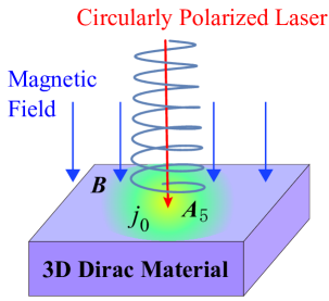
Let us consider a circularly polarized electric field, as depicted in Fig. 15, with the following vector potential:
| (102) |
The corresponding Hamiltonian is periodically time-dependent, i.e.,
| (103) |
with . In the above the whole Hamiltonian is split into a static part, , and the positive- and negative-frequency parts, . The Floquet effective Hamiltonian can be systematically obtained by the expansion if is large enough (only for which the Floquet theory physically makes sense; otherwise, the temperature diverges without prethermalization [95]). Then, there is a formula known as the Magnus expansion [96], from which we can read the first expanded term up to using the above notation, and , as
| (104) |
with . Now we understand that we can regard this last term as an induced axial vector potential, .
Because is transformed into , the modified Gauss law (87) indicates that a finite charge density is pumped up (i.e., chiral pumping effect) as
| (105) |
coupled with a magnetic field, , which can be derived also from direct calculations [94].
The effect of circularly polarized electric field mimics rotational effect, which can be better understood in the following manner. Instead of a combination of circularly polarized electric field and static magnetic field, let us consider just a rotating magnetic field which produces periodically driven potential. We can eliminate time dependence by the coordinate transformation:
| (106) |
Then, the Floquet transformation of the basis,
| (107) |
with the replacement of with the Vierbein reduces the problem into a static one characterized by the transformed Lagrangian density:
| (108) |
Now, we see that a rotating magnetic field is transformed into a static one, as expected from the frame change, and the effect is not only that but also the transformation gives rise to a new term, which can be identified with the axial vector potential corresponding to , leading to [78]
| (109) |
In this case the above result assumes no approximation, which makes a sharp contrast to the previous calculation based on the Magnus expansion. This exactness of resulting is explained by the anomaly nature as argued in Ref. [97] where the same expression was obtained.
4.2.2 Interpretation as an artificial electric field
The Floquet theory has an interesting interpretation in physics, as slightly mentioned in a review [98], which has much to do with the main subject of this article. We will briefly look over the basic idea of what is called Sambe space [99].
The periodic Hamiltonian has a Fourier expanded form,
| (110) |
with . The Floquet state having a quasi-energy, , can be also Fourier expanded as
| (111) |
Then, the eigenvalue equation to determine the quasi-eigenenergy and the Floquet basis states reads:
| (112) |
In Floquet picture this eigenvalue equation is given an interesting interpretation. The matrix representation of the quasi-energy operator in the left-hand side has diagonal components, , , , and these states are communicated by off-diagonal interactions, , . Then, along the Floquet direction labeled by , the diagonal Hamiltonian has an energy slope by . If we regard this Floquet direction as an extra spatial axis, we can identify the energy shift, , as a coordinate dependent static potential. Therefore, the slope of the energy shift is nothing but a static electric field (one more mass dimension should be compensated by “lattice spacing” which is arbitrary in the present description). This picture of fictitious electric field is useful, for example, to think of topological aspects in Floquet systems.
It would be a fascinating possibility to emulate effects equivalent to in (3+1) dimensions without using but with just time periodic perturbations onto a system in (2+1) dimensions. Such a connection between the Floquet system and the finite- system should deserve more investigations from both theoretical and experimental sides.
4.3 Relativistic Gyromagnetic Effects
The CVE is an axial vector current induced by rotation, as we have already seen, and the axial vector is translated to a spin expectation value in the non-relativistic limit. Actually, in non-relativistic theories, it is a well established notion that a finite orbital angular momentum of mechanical rotation can be transported into a finite spin, which is known as the Barnett effect. The Barnett effect is an inverse phenomenon of the Einstein–de Haas effect, and these effects are manifestations of more general gyromagnetic effects as summarized in Ref. [12]. Then, conversely, it would be a natural anticipation to associate the CVE with a relativistic extension of the Barnett effect. However, there are still some unresolved issues, and so this section must remain speculative.
4.3.1 Chiral Barnett effect
The Barnett effect is quantified by a formula connecting the magnetization, , and the angular velocity vector, . A quick derivation of the formula is found in Ref. [12], which can be readily understood in terms of the energy shift. The angular momentum, , makes an energy shift by , which is equated to the magnetic energy shift by with the magnetic moment and the effective magnetic field . The magnetization is with the magnetic susceptibility and the magnetic moment is with the gyromagnetic ratio . Then, and can be eliminated, that is, the standard formula for the non-relativistic Barnett effect obtains as
| Barnett Effect: A finite magnetization, , along the rotation axis appears for a net charge neutral object spun with the angular velocity , which is formulated as (113) |
The gyromagnetic ratio of free fermion reads as with the electric charge and the mass together with a -factor. Then, the magnetization is proportional to the mass, and thus the Barnett effect becomes more prominent with larger mass, which motivates the observation of the nuclear Barnett effect.
In contrast to heavy mass enhancement, in relativistic generalization for light particles, the most subtle part is the decomposition of the angular momentum into the orbital and the spin components. What is conserved as a Nöther current is the total angular momentum only, which is immediately found from the Dirac Lagrangian as
| (114) |
It is quite natural, in a sense that the non-relativistic limit is smoothly taken, to consider the first two terms involving the coordinates as the orbital angular momentum and the rest as the spin. Then, this identification leads to , that is, the axial vector current itself is the spin. With this hypothetical identification, the spin expectation value is expressed for a given distribution function as studied in Ref. [100]. The answer up to the first order in the expansion and also the expansion has two contributions:
| (115) |
This expression uses a little sloppy notation. The subscript denotes a contribution from one-handed fermion sector. The first term is a part of the CVE current as given in Eq. (94). This induced spin expectation value yields a finite magnetic moment, so that the longitudinal magnetization is concluded, which is a natural relativistic extension of the conventional Barnett effect.
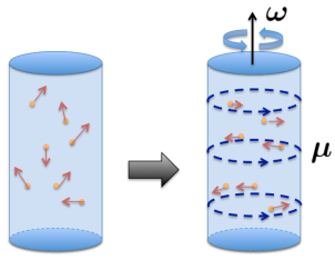
The physical interpretation of the second term proportional to , which is denoted here by , is highly nontrivial. To clarify the intuitive meaning, it would be useful to reexpress it as
| (116) |
where we see that represents the transverse velocity of rotating matter. Because right-handed (left-handed) fermions have the spin alignment in parallel (anti-parallel) to the momentum direction, therefore, this transverse Barnett effect is an inevitable consequence from a combination of chiral imbalance and rotation as graphically shown in Fig. 16. It should be noted that analogous nontrivial effects as results of spin-rotation coupling have been predicted in a different context [101]. So far, this transverse Barnett effect for relativistic fermions is only a theory conjecture, and more studies await.
4.3.2 Chiral Einstein–de Haas effect
The essence for the Einstein–de Haas effect is the angular momentum conservation. That is, the spin relaxation results in a finite amount of the orbital angular momentum so that the total angular momentum must be conserved. Because the orbital angular momentum is associated with mechanical rotation, such a transported orbital momentum causes a physical rotation. In this sense, the conservation law is robust, and the relativistic extension should be straightforward.
To concretize the physical setup, let us suppose chiral matter at rest (i.e., no rotation yet). Then, a finite magnetic field is adiabatically introduced into the system. A finite spin expectation value grows up in response to imposed magnetic field. Actually, the magnetic field itself applied to charged particles carries a finite angular momentum as argued in Ref. [102], which makes the realization of conservation law a little complicated. Once the spin operator in relativistic theory is identified as the axial vector current, it is a classically conserved quantity for chiral matter with . This means that, without - and -violating electromagnetic background, therefore, the integrated spin averaged over the whole system should be vanishing, and so the angular momentum of the magnetic field cannot be received by the spin but may be maximally transferred to the orbital angular momentum only, leading to an enhancement in the Einstein–de Haas effect. This conjecture still awaits to be formulated and quantified by field-theoretical investigations. One may think that the field-theoretical calculations are just straightforward, but in practice, there appear nontrivial subtleties in renormalization. Up to now, to the best of my knowledge, no successful calculation has been reported yet.
5 Summary
As excused in the beginning, this review is not a summarizing report to cover all related works with balanced weights, but it is more like a story along a history of my own research interest. The order of sections, subsections, subsubsections, therefore, has inevitability for me as if the order of all historical events had definite inevitability. I must apologize for not mentioning all relevant works, which is in any case impossible.
The magnetic catalysis is the most important phenomenon of chiral matter put in magnetic field. Because there are already very nice review articles to explicate the basics and the applications, I tried to give only minimal but reproducible calculations. The essential point is that the vacuum in quantum field theories is more like a medium in condensed matter physics and it is affected by environments such as external magnetic fields. There may be a phase transition triggered by the magnetic field, and/or, the existing phase transitions points are shifted by imposed magnetic field. All these have profound implications in nuclear physics as well as in other fields. To make this review pedagogical and self-contained, I could not refer to some interesting ideas such as superconductivity of the vacuum induced by the magnetic field [103], which is an extremely interesting idea. As mentioned above, usually, the magnetic field influences medium properties, but conversely, the magnetic field in Ref. [103] plays a role of medium. In fact, such a view of the magnetic field as a medium can be traced back to old discussions on the birefringence in the magnetic field and/or the photon splitting problem under strong magnetic field. In this review I tried to spell out calculation procedures especially in the early sections, so that readers can reproduce the main results, and if necessary, can make use of the method for further applications. Because all algebraic elements are given, readers are armed with theoretical tools, and ready to attack advanced problems as listed above if interested.
I would like to stress one point. For practical purposes Schwinger’s proper-time integral is the most convenient approach, but I preferred to start with explicit solutions of the free Dirac equation. This is because the complete set of wave-functions contains more detailed information than the propagator. For example, to take account of finite size effect, the most straightforward strategy is to solve the Dirac equation under a boundary condition. Also, for problems with finite rotation, this rather brute-force method is useful to impose the causality condition. Such explicit construction of wave-functions is also beneficial in order to think of new chiral effects. In short, anything interesting inherent to chirality is caused by helical structures. The matter chirality can indicate a helical motion, a special optical setup may involve a helical magnetic profile, a screw type rotation pumps charges up, etc. Then, the wave-functions can directly visualize the mechanism.
Everybody would agree that the inclusion of electric field is the next step after treating magnetic fields. The problem, however, becomes much more difficult by orders of magnitude. This is so because the problem cannot be static any longer but should be dynamical as soon as the external electric field is involved, which can be alternatively understood as the sign problem in numerical Monte-Carlo simulations. Thus, phase diagrams with an axis of external magnetic field can exist, while matter exposed to external electric field cannot be classified into equilibrated distinct phases.
A new element brought in by electric field is the particle production from quantum fluctuations. In a sense the vacuum in quantum field theory should be not an empty state but more like a medium, as emphasized above, and the particle production from the vacuum, known as the Schwinger Mechanism, is a phenomenon of insulator-metal transition in solid state physics. Although inclusion of the magnetic field on phase diagram research becase quite fashionable and a countless number of publications appear especially for the strongly interacting system of quarks and gluons, not many papers address the electric effect so far. This is because of technical difficulties; the physics must be rich, but the calculation costs too much. This is the reason why I introduced, in this review, a relatively unknown machinery for the electric calculus of Ref. [61]. The inclusion of the electric field in real time deforms the proper-time path, in a similar way as the finite-temperature field theory. In a sense we can say that the finite electric theory looks like a holographic higher dimensional theory in which a quantum axis is treated as if the temporal axis in the ordinary finite temperature field theory. This correspondence is quite suggestive; it is a longstanding puzzle whether the Schwinger Mechanism is thermal or not. Physics wise, the Schwinger Mechanism and the Unruh effect are very similar, but the latter has a clear interpretation of the vacuum as a thermal bath. Why not the former? Of course, a boring answer is that the mass dimension of the electric field is not one but two. It should be worth mentioning that the proper time has a mass dimension negative two, and this fact suggests that the thermal interpretation may emerge in terms of the proper time, for which the formulation of Ref. [61] might tell us a hint.
The last part of this review is about some ongoing research projects on the relativistic generalization of classic themes, namely, the Barnett effect and the Einstein–de Haas effect. Usually the Barnett effect is proportional to the mass (since the gyromagnetic ratio is inversely proportional to the mass), heavier particles like nuclei would be more desirable than lighter particles like electrons for experimental observation. However, at the same time, the spin-orbit coupling is a relativistic effect, and it should be enhanced for chiral fermions. Then, it is a highly nontrivial question whether such gyromagnetic effects are enhanced or suppressed when the physical system transits from the non-relativistic to the ultra-relativistic limit. This part still awaits further theoretical and experimental investigations. In this way, this review is not a standard review to rephrase established facts, but I dared to include unmatured topics, hoping that they are seeds for rich harvest on the next level in the near future.
Acknowledgments
The author thanks Hao-Lei Chen, Patrick Copinger, Shu Ebihara, Antonino Flachi, Francois Gelis, Yoshimasa Hidaka, Xu-Guang Huang, Dmitri Kharzeev, Tuomas Lappi, Kazuya Mameda, Takashi Oka, Jan Pawlowski, Shi Pu, Zebin Qiu, Harmen Warringa for discussions and collaborations. The author learnt a lot from collaborations with them, and this review is based on papers coauthored with them.
In the discussions on the magnetic catalysis I gave rather detailed explanations in terms of the renormalization group. The physical contents are equivalent to direct calculations but such an intuitive view to understand physics is quite interesting. Actually, I learnt this RG argument from Jan Pawlowski who is an expert on the functional RG approach, and then I felt like that my eyes were reopened to a new streak of light. I hope that some readers may find this RG argument inspiring as I once did.
In the presence of both electric and magnetic fields, interestingly, such background fields break - and -symmetries, and the particle–anti-particle symmetry is violated then. This violation causes an unbalanced distribution of chirality, that is, a finite difference between right-handed and left-handed particles. This kind of chiral unbalanced matter under magnetic field is an ideal device to realize the chiral magnetic effect. Regarding the physical interpretation, since when Dmitri Kharzeev, Harmen Warringa, and I published a paper on the CME, it had been a puzzle how to distinguish the genuine current in real time and the Euclidean and thus static expectation value of the current operator. For example, in lattice discretized numerical simulation as done by Arata Yamamoto, it is always possible to measure the current operator expectation value, but such Euclidean formulation cannot be a proper description of real-time phenomena. After 10 years since our paper on the CME, I believe that, thanks to collaboration with Patrick Copinger and Shi Pu, I eventually reached a clear way to understand the difference between the Minkowskian and the Euclidean quantities using the in- and out-states. I would emphasize that using the chiral chemical potential, , which is a great invention by Harmen, is a very convenient bookkeeping device, but, if controversies are fomented by , an alternative and more physical formulation with would be helpful to resolve confusions.
Analogy between the magnetic field and the rotation is another longstanding problem. I learnt a lot about the Floquet theory from Takashi Oka and was convinced that the Floquet engineering is such a promising technique to test various ideas of relativistic quantum field theory including the quantum anomaly. With this technique, even theory fictions like axial vector potentials can be implemented in real experiments. Now, the applications of synthetic magnetic field (aka, artificial gauge potential) have been a wide spreading subject, and it is not a radical idea at all to expect some Floquet engineering suited for studies on the CME and the analogous phenomena, e.g., the chiral vortical effect. Along these directions I am (trying to) keeping touch with Takashi and another Floquet expert, André Eckardt, from whom I learnt as much.
I could continue my personal memories endlessly, but now, let me finally close the review, stating that this work was supported by JSPS KAKENHI Grant No. 18H01211.
References
- [1] D. Lai, “Matter in strong magnetic fields,” Rev. Mod. Phys. 73 (2001) 629–662.
- [2] V. A. Miransky and I. A. Shovkovy, “Quantum field theory in a magnetic field: From quantum chromodynamics to graphene and Dirac semimetals,” Phys. Rept. 576 (2015) 1–209, arXiv:1503.00732 [hep-ph].
- [3] K. Hattori and X.-G. Huang, “Novel quantum phenomena induced by strong magnetic fields in heavy-ion collisions,” Nucl. Sci. Tech. 28 (2017) 26, arXiv:1609.00747 [nucl-th].
- [4] D. E. Kharzeev, J. Liao, S. A. Voloshin, and G. Wang, “Chiral magnetic and vortical effects in high-energy nuclear collisions-A status report,” Prog. Part. Nucl. Phys. 88 (2016) 1–28, arXiv:1511.04050 [hep-ph].
- [5] G. V. Dunne, “Heisenberg-Euler effective Lagrangians: Basics and extensions,” in From fields to strings: Circumnavigating theoretical physics. Ian Kogan memorial collection (3 volume set), M. Shifman, A. Vainshtein, and J. Wheater, eds., pp. 445–522. 2004. arXiv:hep-th/0406216 [hep-th].
- [6] F. Gelis and N. Tanji, “Schwinger mechanism revisited,” Prog. Part. Nucl. Phys. 87 (2016) 1–49, arXiv:1510.05451 [hep-ph].
- [7] K. Fukushima, “Views of the chiral magnetic effect,” Lect. Notes Phys. 871 (2013) 241–259, arXiv:1209.5064 [hep-ph].
- [8] P.-G. de Gennes, Superconductivity of Metals and Alloys. Advanced book classics. Advanced Book Program, Perseus Books, 1999.
- [9] W. Domcke, P. Hänggi, and D. Tannor, “Driven Quantum Systems,” Special Issue : Chem. Phys. 217 (1997) 117–416.
- [10] M. Bukov, L. D’Alessio, and A. Polkovnikov, “Universal high-frequency behavior of periodically driven systems: from dynamical stabilization to floquet engineering,” Advances in Physics 64 (2015) 139–226.
- [11] J. Dalibard, F. Gerbier, G. Juzeliūnas, and P. Öhberg, “Colloquium: Artificial gauge potentials for neutral atoms,” Rev. Mod. Phys. 83 (2011) 1523–1543.
- [12] S. J. Barnett, “Gyromagnetic and electron-inertia effects,” Rev. Mod. Phys. 7 (1935) 129–166.
- [13] V. Ritus, “Radiative corrections in quantum electrodynamics with intense field and their analytical properties,” Annals of Physics 69 (1972) 555 – 582.
- [14] J. L. Noronha and I. A. Shovkovy, “Color-flavor locked superconductor in a magnetic field,” Phys. Rev. D76 (2007) 105030, arXiv:0708.0307 [hep-ph]. [Erratum: Phys. Rev.D86,049901(2012)].
- [15] K. Fukushima, D. E. Kharzeev, and H. J. Warringa, “Electric-current susceptibility and the chiral magnetic effect,” Nucl. Phys. A836 (2010) 311–336, arXiv:0912.2961 [hep-ph].
- [16] J. S. Schwinger, “On gauge invariance and vacuum polarization,” Phys. Rev. 82 (1951) 664–679.
- [17] V. P. Gusynin, V. A. Miransky, and I. A. Shovkovy, “Dimensional reduction and dynamical chiral symmetry breaking by a magnetic field in (3+1)-dimensions,” Phys. Lett. B349 (1995) 477–483, arXiv:hep-ph/9412257 [hep-ph].
- [18] V. P. Gusynin, V. A. Miransky, and I. A. Shovkovy, “Dimensional reduction and catalysis of dynamical symmetry breaking by a magnetic field,” Nucl. Phys. B462 (1996) 249–290, arXiv:hep-ph/9509320 [hep-ph].
- [19] K. Fukushima and Y. Hidaka, “Magnetic catalysis versus magnetic inhibition,” Phys. Rev. Lett. 110 (2013) 031601, arXiv:1209.1319 [hep-ph].
- [20] Y. Nambu and G. Jona-Lasinio, “Dynamical model of elementary particles based on an analogy with superconductivity I,” Phys. Rev. 122 (1961) 345–358.
- [21] H. Suganuma and T. Tatsumi, “On the behavior of symmetry and phase transitions in a strong electromagnetic field,” Annals Phys. 208 (1991) 470–508.
- [22] I. A. Shushpanov and A. V. Smilga, “Quark condensate in a magnetic field,” Phys. Lett. B402 (1997) 351–358, arXiv:hep-ph/9703201 [hep-ph].
- [23] T. D. Cohen, D. A. McGady, and E. S. Werbos, “The Chiral condensate in a constant electromagnetic field,” Phys. Rev. C76 (2007) 055201, arXiv:0706.3208 [hep-ph].
- [24] V. P. Gusynin, V. A. Miransky, and I. A. Shovkovy, “Catalysis of dynamical flavor symmetry breaking by a magnetic field in (2+1)-dimensions,” Phys. Rev. Lett. 73 (1994) 3499–3502, arXiv:hep-ph/9405262 [hep-ph]. [Erratum: Phys. Rev. Lett.76,1005(1996)].
- [25] S. P. Klevansky, “The Nambu-Jona-Lasinio model of quantum chromodynamics,” Rev. Mod. Phys. 64 (1992) 649–708.
- [26] T. Hatsuda and T. Kunihiro, “QCD phenomenology based on a chiral effective Lagrangian,” Phys. Rept. 247 (1994) 221–367, arXiv:hep-ph/9401310 [hep-ph].
- [27] D. D. Scherer and H. Gies, “Renormalization group study of magnetic catalysis in the 3d Gross-Neveu model,” Phys. Rev. B85 (2012) 195417, arXiv:1201.3746 [cond-mat.str-el].
- [28] K. Fukushima and J. M. Pawlowski, “Magnetic catalysis in hot and dense quark matter and quantum fluctuations,” Phys. Rev. D86 (2012) 076013, arXiv:1203.4330 [hep-ph].
- [29] F. Preis, A. Rebhan, and A. Schmitt, “Inverse magnetic catalysis in dense holographic matter,” JHEP 03 (2011) 033, arXiv:1012.4785 [hep-th].
- [30] F. Preis, A. Rebhan, and A. Schmitt, “Inverse magnetic catalysis in field theory and gauge-gravity duality,” Lect. Notes Phys. 871 (2013) 51–86, arXiv:1208.0536 [hep-ph].
- [31] G. S. Bali, F. Bruckmann, G. Endrodi, Z. Fodor, S. D. Katz, S. Krieg, A. Schafer, and K. K. Szabo, “The QCD phase diagram for external magnetic fields,” JHEP 02 (2012) 044, arXiv:1111.4956 [hep-lat].
- [32] K. Fukushima, “Chiral effective model with the Polyakov loop,” Phys. Lett. B591 (2004) 277–284, arXiv:hep-ph/0310121 [hep-ph].
- [33] C. Ratti, M. A. Thaler, and W. Weise, “Phases of QCD: Lattice thermodynamics and a field theoretical model,” Phys. Rev. D73 (2006) 014019, arXiv:hep-ph/0506234 [hep-ph].
- [34] A. J. Mizher, M. N. Chernodub, and E. S. Fraga, “Phase diagram of hot QCD in an external magnetic field: possible splitting of deconfinement and chiral transitions,” Phys. Rev. D82 (2010) 105016, arXiv:1004.2712 [hep-ph].
- [35] R. Gatto and M. Ruggieri, “Quark Matter in a Strong Magnetic Background,” Lect. Notes Phys. 871 (2013) 87–119, arXiv:1207.3190 [hep-ph].
- [36] G. S. Bali, F. Bruckmann, G. Endrodi, Z. Fodor, S. D. Katz, and A. Schafer, “QCD quark condensate in external magnetic fields,” Phys. Rev. D86 (2012) 071502, arXiv:1206.4205 [hep-lat].
- [37] G. S. Bali, F. Bruckmann, G. Endrodi, F. Gruber, and A. Schaefer, “Magnetic field-induced gluonic (inverse) catalysis and pressure (an)isotropy in QCD,” JHEP 04 (2013) 130, arXiv:1303.1328 [hep-lat].
- [38] K. Fukushima, “Magnetic-field induced screening effect and collective excitations,” Phys. Rev. D83 (2011) 111501, arXiv:1103.4430 [hep-ph].
- [39] K. Hattori and K. Itakura, “Vacuum birefringence in strong magnetic fields: (I) Photon polarization tensor with all the Landau levels,” Annals Phys. 330 (2013) 23–54, arXiv:1209.2663 [hep-ph].
- [40] K. Hattori and K. Itakura, “Vacuum birefringence in strong magnetic fields: (II) Complex refractive index from the lowest Landau level,” Annals Phys. 334 (2013) 58–82, arXiv:1212.1897 [hep-ph].
- [41] F. Bruckmann, G. Endrodi, and T. G. Kovacs, “Inverse magnetic catalysis and the Polyakov loop,” JHEP 04 (2013) 112, arXiv:1303.3972 [hep-lat].
- [42] E. J. Ferrer, V. de la Incera, and X. J. Wen, “Quark Antiscreening at Strong Magnetic Field and Inverse Magnetic Catalysis,” Phys. Rev. D91 (2015) no. 5, 054006, arXiv:1407.3503 [nucl-th].
- [43] N. Mueller and J. M. Pawlowski, “Magnetic catalysis and inverse magnetic catalysis in QCD,” Phys. Rev. D91 (2015) 116010, arXiv:1502.08011 [hep-ph].
- [44] G. Endrödi, “QCD equation of state at nonzero magnetic fields in the Hadron Resonance Gas model,” JHEP 04 (2013) 023, arXiv:1301.1307 [hep-ph].
- [45] K. Fukushima and Y. Hidaka, “Magnetic shift of the chemical freeze-out and electric charge fluctuations,” Phys. Rev. Lett. 117 (2016) no. 10, 102301, arXiv:1605.01912 [hep-ph].
- [46] F. Sauter, “Zum Kleinschen Paradoxon,” Z. Phys. 73 (1932) 547–552.
- [47] D. Cangemi, E. D’Hoker, and G. V. Dunne, “Effective energy for QED in (2+1)-dimensions with semilocalized magnetic fields: A Solvable model,” Phys. Rev. D52 (1995) R3163–R3167, arXiv:hep-th/9506085 [hep-th].
- [48] Y. Aharonov and A. Casher, “Ground state of a spin-1/2 charged particle in a two-dimensional magnetic field,” Phys. Rev. A 19 (1979) 2461–2462.
- [49] P. Copinger and K. Fukushima, “Spatially assisted Schwinger Mechanism and magnetic catalysis,” Phys. Rev. Lett. 117 (2016) 081603, arXiv:1605.05957 [hep-th]. [Erratum: Phys. Rev. Lett.118,no.9,099903(2017)].
- [50] H.-L. Chen, K. Fukushima, X.-G. Huang, and K. Mameda, “Surface magnetic catalysis,” Phys. Rev. D96 (2017) 054032, arXiv:1707.09130 [hep-ph].
- [51] J. Schwinger, “On gauge invariance and vacuum polarization,” Phys. Rev. 82 (1951) 664–679.
- [52] T. D. Cohen and D. A. McGady, “The Schwinger mechanism revisited,” Phys. Rev. D78 (2008) 036008, arXiv:0807.1117 [hep-ph].
- [53] C. Itzykson and J. Zuber, Quantum Field Theory. International series in pure and applied physics. McGraw-Hill, 1985.
- [54] K. Fukushima, F. Gelis, and T. Lappi, “Multiparticle correlations in the Schwinger mechanism,” Nucl. Phys. A831 (2009) 184–214, arXiv:0907.4793 [hep-ph].
- [55] G. ’t Hooft, “The Scattering matrix approach for the quantum black hole: An Overview,” Int. J. Mod. Phys. A11 (1996) 4623–4688, arXiv:gr-qc/9607022 [gr-qc].
- [56] A. I. Nikishov, “Barrier scattering in field theory removal of klein paradox,” Nucl. Phys. B21 (1970) 346–358.
- [57] N. Tanji, “Dynamical view of pair creation in uniform electric and magnetic fields,” Annals Phys. 324 (2009) 1691–1736, arXiv:0810.4429 [hep-ph].
- [58] C. Schubert, “Perturbative quantum field theory in the string inspired formalism,” Phys. Rept. 355 (2001) 73–234, arXiv:hep-th/0101036 [hep-th].
- [59] R. Schutzhold, H. Gies, and G. Dunne, “Dynamically assisted Schwinger mechanism,” Phys. Rev. Lett. 101 (2008) 130404, arXiv:0807.0754 [hep-th].
- [60] H. B. Nielsen and M. Ninomiya, “Adler-Bell-Jackiw anomaly and Weyl fermions in crystal,” Phys. Lett. 130B (1983) 389–396.
- [61] E. Fradkin, D. Guitman, and S. Shvartsman, Quantum electrodynamics: with unstable vacuum. Springer series in nuclear and particle physics. Springer-Verlag, 1991.
- [62] P. Copinger, K. Fukushima, and S. Pu, “Axial Ward identity and the Schwinger mechanism – Applications to the real-time chiral magnetic effect and condensates,” arXiv:1807.04416 [hep-th].
- [63] H. J. Warringa, “Dynamics of the Chiral Magnetic Effect in a weak magnetic field,” Phys. Rev. D86 (2012) 085029, arXiv:1205.5679 [hep-th].
- [64] F. Wilczek, “Two applications of axion electrodynamics,” Phys. Rev. Lett. 58 (1987) 1799.
- [65] K. Fukushima, D. E. Kharzeev, and H. J. Warringa, “The Chiral Magnetic Effect,” Phys. Rev. D78 (2008) 074033, arXiv:0808.3382 [hep-ph].
- [66] A. Vilenkin, “Equilibrium parity violating current in a magnetic field,” Phys. Rev. D22 (1980) 3080–3084.
- [67] M. Giovannini and M. Shaposhnikov, “Primordial magnetic fields, anomalous isocurvature fluctuations and big bang nucleosynthesis,” Phys. Rev. Lett. 80 (1998) 22–25, arXiv:hep-ph/9708303 [hep-ph].
- [68] M. M. Vazifeh and M. Franz, “Electromagnetic response of weyl semimetals,” Phys. Rev. Lett. 111 (2013) 027201.
- [69] N. Yamamoto, “Generalized Bloch theorem and chiral transport phenomena,” Phys. Rev. D92 (2015) no. 8, 085011, arXiv:1502.01547 [cond-mat.mes-hall].
- [70] K. Fukushima, D. E. Kharzeev, and H. J. Warringa, “Real-time dynamics of the Chiral Magnetic Effect,” Phys. Rev. Lett. 104 (2010) 212001, arXiv:1002.2495 [hep-ph].
- [71] D. T. Son and B. Z. Spivak, “Chiral anomaly and classical negative magnetoresistance of Weyl metals,” Phys. Rev. B88 (2013) 104412, arXiv:1206.1627 [cond-mat.mes-hall].
- [72] Q. Li, D. E. Kharzeev, C. Zhang, Y. Huang, I. Pletikosic, A. V. Fedorov, R. D. Zhong, J. A. Schneeloch, G. D. Gu, and T. Valla, “Observation of the chiral magnetic effect in ZrTe5,” Nature Phys. 12 (2016) 550–554, arXiv:1412.6543 [cond-mat.str-el].
- [73] K. Fukushima and Y. Hidaka, “Electric conductivity of hot and dense quark matter in a magnetic field with Landau level resummation via kinetic equations,” Phys. Rev. Lett. 120 (2018) no. 16, 162301, arXiv:1711.01472 [hep-ph].
- [74] Y. Jiang and J. Liao, “Pairing phase transitions of matter under rotation,” Phys. Rev. Lett. 117 (2016) no. 19, 192302, arXiv:1606.03808 [hep-ph].
- [75] M. N. Chernodub and S. Gongyo, “Effects of rotation and boundaries on chiral symmetry breaking of relativistic fermions,” Phys. Rev. D95 (2017) no. 9, 096006, arXiv:1702.08266 [hep-th].
- [76] Y. Liu and I. Zahed, “Pion condensation by rotation in a magnetic field,” Phys. Rev. Lett. 120 (2018) no. 3, 032001, arXiv:1711.08354 [hep-ph].
- [77] H.-L. Chen, K. Fukushima, X.-G. Huang, and K. Mameda, “Analogy between rotation and density for Dirac fermions in a magnetic field,” Phys. Rev. D93 (2016) no. 10, 104052, arXiv:1512.08974 [hep-ph].
- [78] S. Ebihara, K. Fukushima, and K. Mameda, “Boundary effects and gapped dispersion in rotating fermionic matter,” Phys. Lett. B764 (2017) 94–99, arXiv:1608.00336 [hep-ph].
- [79] F. Becattini and L. Tinti, “The Ideal relativistic rotating gas as a perfect fluid with spin,” Annals Phys. 325 (2010) 1566–1594, arXiv:0911.0864 [gr-qc].
- [80] A. Vilenkin, “Parity violating currents in thermal radiation,” Phys. Lett. 80B (1978) 150–152.
- [81] A. Vilenkin, “Macroscopic parity violating effects: neutrino fluxes from rotating black holes and in rotating thermal radiation,” Phys. Rev. D20 (1979) 1807–1812.
- [82] A. Vilenkin, “Quantum field theory at finite temperature in a rotating system,” Phys. Rev. D21 (1980) 2260–2269.
- [83] K. Landsteiner, E. Megias, and F. Pena-Benitez, “Gravitational anomaly and transport,” Phys. Rev. Lett. 107 (2011) 021601, arXiv:1103.5006 [hep-ph].
- [84] K. Landsteiner, E. Megias, L. Melgar, and F. Pena-Benitez, “Holographic gravitational anomaly and chiral vortical effect,” JHEP 09 (2011) 121, arXiv:1107.0368 [hep-th].
- [85] K. Jensen, R. Loganayagam, and A. Yarom, “Thermodynamics, gravitational anomalies and cones,” JHEP 02 (2013) 088, arXiv:1207.5824 [hep-th].
- [86] K. Jensen, R. Loganayagam, and A. Yarom, “Anomaly inflow and thermal equilibrium,” JHEP 05 (2014) 134, arXiv:1310.7024 [hep-th].
- [87] S. Golkar and D. T. Son, “(Non)-renormalization of the chiral vortical effect coefficient,” JHEP 02 (2015) 169, arXiv:1207.5806 [hep-th].
- [88] S. Golkar and S. Sethi, “Global anomalies and effective field theory,” JHEP 05 (2016) 105, arXiv:1512.02607 [hep-th].
- [89] D. T. Son and P. Surowka, “Hydrodynamics with triangle anomalies,” Phys. Rev. Lett. 103 (2009) 191601, arXiv:0906.5044 [hep-th].
- [90] M. Buzzegoli, E. Grossi, and F. Becattini, “General equilibrium second-order hydrodynamic coefficients for free quantum fields,” JHEP 10 (2017) 091, arXiv:1704.02808 [hep-th]. [Erratum: JHEP07,119(2018)].
- [91] A. Flachi and K. Fukushima, “Chiral vortical effect with finite rotation, temperature, and curvature,” Phys. Rev. D98 (2018) no. 9, 096011, arXiv:1702.04753 [hep-th].
- [92] A. Flachi and K. Fukushima, “Chiral mass-gap in curved space,” Phys. Rev. Lett. 113 (2014) no. 9, 091102, arXiv:1406.6548 [hep-th].
- [93] M. N. Chernodub, A. Cortijo, and K. Landsteiner, “Zilch vortical effect,” Phys. Rev. D98 (2018) no. 6, 065016, arXiv:1807.10705 [hep-th].
- [94] S. Ebihara, K. Fukushima, and T. Oka, “Chiral pumping effect induced by rotating electric fields,” Phys. Rev. B93 (2016) no. 15, 155107, arXiv:1509.03673 [cond-mat.str-el].
- [95] T. Mori, T. Kuwahara, and K. Saito, “Rigorous bound on energy absorption and generic relaxation in periodically driven quantum systems,” Phys. Rev. Lett. 116 (2016) 120401.
- [96] S. Blanes, F. Casas, J. Oteo, and J. Ros, “The magnus expansion and some of its applications,” Physics Reports 470 (2009) no. 5, 151 – 238.
- [97] K. Hattori and Y. Yin, “Charge redistribution from anomalous magnetovorticity coupling,” Phys. Rev. Lett. 117 (2016) no. 15, 152002, arXiv:1607.01513 [hep-th].
- [98] T. Oka and S. Kitamura, “Floquet engineering of quantum materials,” Annual Review of Condensed Matter Physics 10 (2019) no. 1, 387–408.
- [99] H. Sambe, “Steady states and quasienergies of a quantum-mechanical system in an oscillating field,” Phys. Rev. A 7 (1973) 2203–2213.
- [100] K. Fukushima, S. Pu, and Z. Qiu, “Eddy magnetization from the chiral Barnett effect,” arXiv:1808.08016 [hep-ph].
- [101] M. Matsuo, J. Ieda, E. Saitoh, and S. Maekawa, “Effects of mechanical rotation on spin currents,” Phys. Rev. Lett. 106 (2011) 076601.
- [102] C. R. Greenshields, R. L. Stamps, S. Franke-Arnold, and S. M. Barnett, “Is the angular momentum of an electron conserved in a uniform magnetic field?,” Phys. Rev. Lett. 113 (2014) 240404.
- [103] M. N. Chernodub, “Spontaneous electromagnetic superconductivity of vacuum in strong magnetic field: evidence from the Nambu–Jona-Lasinio model,” Phys. Rev. Lett. 106 (2011) 142003, arXiv:1101.0117 [hep-ph].