Global diagnostics of ionospheric absorption during X-ray solar flares based on 8-20MHz noise measured by over-the-horizon radars.

Abstract

An analysis of noise attenuation during eighty solar flares between 2013 and 2017 was carried out at frequencies 8-20 MHz using thirty-four SuperDARN radars and the EKB ISTP SB RAS radar. The attenuation was determined on the basis of noise measurements performed by the radars during the intervals between transmitting periods. The location of the primary contributing ground sources of noise was found by consideration of the propagation paths of radar backscatter from the ground. The elevation angle for the ground echoes was determined through a new empirical model. It was used to determine the paths of the noise and the location of its source. The method was particularly well suited for daytime situations which had to be limited for the most part to only two crossings through the D region. Knowing the radio path was used to determine an equivalent vertical propagation attenuation factor. The change in the noise during solar flares was correlated with solar radiation lines measured by GOES/XRS, GOES/EUVS, SDO/AIA, SDO/EVE, SOHO/SEM and PROBA2/LYRA instruments. Radiation in the 1 to 8$\mathring{A}$ and and near 100$\mathring{A}$ are shown to be primarily responsible for the increase in the radionoise absorption, and by inference, for an increase in the D and E region density. The data are also shown to be consistent with a radar frequency dependence having a power law with an exponent of -1.6. This study shows that a new dataset can be made available to study D and E region.

1 Introduction

The monitoring of ionospheric absorption at High Frequency (HF), particularly at high latitudes, makes it feasible to predict radio wave absoption at long distances and therefore on global scales DRAP Documentation (2010); Akmaev, R. A. (2010). This in turn makes it a useful tool for study of the dynamics of the D and E regions. Traditionally, there are several techniques in use Davies (1969); Hunsucker  Hargreaves (2002), including constant power 2-6 MHz transmitters (URSI A1 and A3 methods, see for example Sauer  Wilkinson (2008); Schumer (2010)), riometry using cosmic radio space sources at 30-50 MHz (URSI A2 method Hargreaves (2010)) and imaging riometry Detrick  Rosenberg (1990). Recently, a large, spatially distributed network of riometers has been deployed to monitor absorption Rogers  Honary (2015). The development of new techniques for studying absorption with wide spatial coverage would be valuable for the validation of global ionospheric models and for global absorption forecasting.

A wide network of radio instruments in the HF frequency range is available with the SuperDARN (Super Dual Auroral Radar Network Greenwald . (1995); Chisham . (2007)) radars and radars close to them in terms of design and software Berngardt . (2015). The main task of the SuperDARN network is to measure ionospheric convection. Currently this network is expanding from polar latitudes to mid-latitudes J. Baker . (2007); Ribeiro . (2012) and possibly to equatorial latitudes Lawal . (2018). Regular radar operation with high spatial and temporal resolutions and a wide field-of-view makes them a useful tool for monitoring ionospheric absorption on global scales. The frequency range used by the radars fills a gap between the riometric measurements at 30-50 MHz (URSI A2 method) and radar measurements at 2-6 MHz band (URSI A1, A3 methods). Various methods are being developed for using these radars to study radiowave absorption. One approach is to monitor third-party transmitters Squibb . (2015) and another is to use the signal backscattered from the ground Watanabe  Nishitani (2013); Chakraborty . (2018); Fiori . (2018). In this paper, another method is investigated. It is based on studying the attenuation of HF noise in the area surrounding the radar that is measured without transmitting any sounding pulses.

Every several seconds, before transmitting at the operating frequency, the radar measures the spectrum of the background noise in a 300-500 kHz band centered on a planned operating frequency that lies between 8-20 MHz. The minimum in the spectral intensity is recorded and defined here as the ’minimal HF noise level’.

Berngardt . (2018) showed that the dynamics of the minimal HF noise level is strongly influenced by X-ray 1-8$\mathring{A}$ solar radiation in the daytime. This effect has also been observed during solar proton events Bland . (2018) where it was found to correlate well with riometer observations. This allows one to use the noise measured with HF radars to investigate the absorption processes in the lower part of the ionosphere in passive mode, without the use of third-party transmitters, and without relying on the presence of backscatter from the ground.

To use this new technique on a regular basis for monitoring ionospheric absorption we should investigate the observed noise level variations during X-ray flares and show that the observed dynamics are consistent with the current absorption models.

As shown in the preliminary analysis Berngardt . (2018), there is significant correlation of noise level attenuation with the intensity of X-ray solar radiation in the range 1-8$\mathring{A}$. However, the temporal dynamics of the absorption sometimes do not precisely track the solar radiation at wavelengths of 1-8$\mathring{A}$, which indicates the presence of mechanisms other than the ionization of the D-layer by 1-8$\mathring{A}$ solar radiation. An example of such a comparison will be presented here in Fig.1A-D and was shown by (Berngardt ., 2018, fig.9).

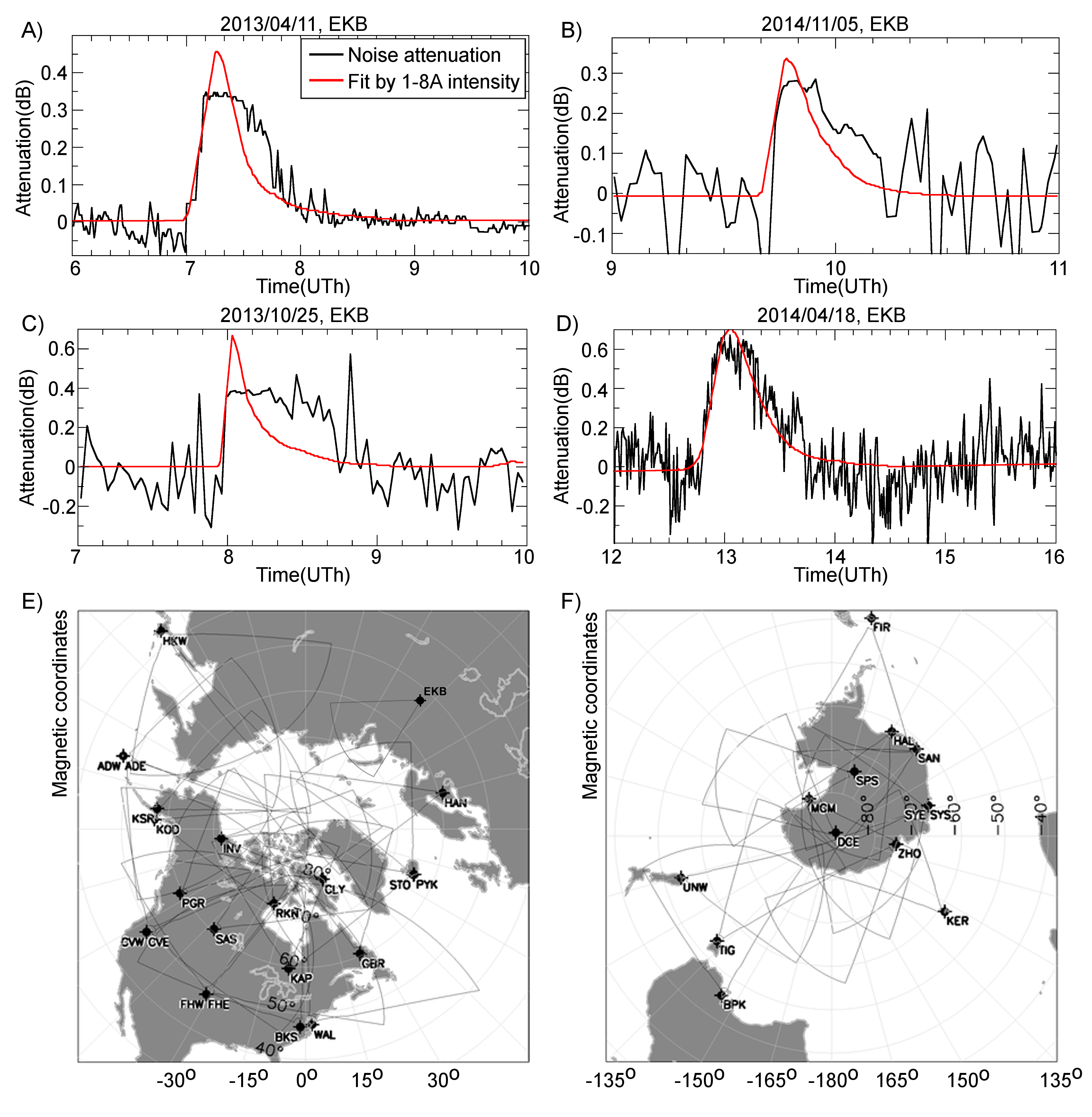
Figure 1: A-D) comparison of the X-ray intensity dynamics measured on GOES/XRS 1-8$\mathring{A}$ and the noise attenuation at EKB ISTP SB RAS radar during four flares; E-F) - fields of views of radars that participated in the work

In contrast to riometers which measure ionospheric absorption at relatively high frequencies (30-50 MHz), the SuperDARN coherent radars use lower operating frequencies and ionospheric refraction significantly affects the absorption level - the trajectory of propagation is distorted by the background ionosphere. To compare the data of different radars during different solar flares, our method requires taking into account the state of the background ionosphere during each experiment. This allows an oblique absorption measurement to be converted to an equivalent vertical measurement. In addition, the solution of this problem allows determination of the geographic location of the region in which the absorption takes place.

Among the factors that affect the error in estimating the absorption level is the frequency at which the radar operates and its irregular switching. It is known that the absorption of radio waves depends on frequency, but this dependence is taken into account in different ways in different papers. In order to make a reliable comparison of data collected from radars operating at different frequencies, it is necessary to find the frequency dependence of the HF noise absorption, and to take it into account. This will allow us to infer the absorption at any frequency from the observed absorption at the radar operating frequency.

The third factor that needs to be taken into account is the altitude localization of the absorption.

The present paper is devoted to solving these problems. An analysis is made of 80 X-ray solar flares during the years 2013-2017 , which were also considered in Berngardt . (2018) based on the available data of 34 high- and mid-latitude radars of SuperDARN network and on the EKB ISTP SB RAS Berngardt . (2015) radar data. The radar locations and their fields of view are shown in fig.1E-F, the radar coordinates are given in the Table LABEL:tab:rad_list. The X-ray solar flares dates are listed in Berngardt . (2018).

2 Taking into account the background ionosphere

As was shown in Berngardt . (2018), during solar X-ray flares attenuation of the minimal noise level in the frequency range 8-20 MHz is observed on the dayside by midlatitude coherent radars. The attenuation correlates with the increase of X-ray solar radiation 1-8$\mathring{A}$ and is associated with the absorption of the radio signal in the lower part of the ionosphere.

The HF radio noise intensity is known to vary with local time due different sources ITU-R P.372-13 (2016). At night, the noise is mostly atmospheric, and is formed by long-range propagation from noise sources around the world, mostly from regions of thunderstorm activity. In the daytime the atmospheric noise level significantly decreases due to regular absorption in the lower part of the ionosphere and the increasing number of propagation hops (caused by increasing electron density and lowering of the radiowave reflection point). As a result, in the daytime the multihop propagation part of the noise becomes small, and only noise sources from the first propagation hop (mostly anthropogenic noise) need to be taken into account Berngardt . (2018).

An important issue related to the interpretation of the noise level is the spatial localization of the effect. It can be estimated by taking into account the radiowave trajectory along which most of the noise is received and absorption is taking place. We will argue that ionization of the lower ionosphere is small enough and skip distance variability is less pronounced than the variations caused by other regular and irregular ionospheric variations.

Let us consider the problem of detecting the noise source from the data of a HF coherent radar. It is known that the intensity of the signal transmitted by an isotropic source and propagating in an inhomogeneous ionosphere substantially depends on the ground distance from the signal transmitter to receiver. If we consider only waves reflecting from the ionosphere, then at sounding frequencies above $foF2$ there is a spatial region where the signal cannot be received - the dead zone. At the boundary of this dead zone (skip distance) the signal appears and is significantly enhanced compared to other distances Shearman (1956); Bliokh . (1988).

More specifically, consider that, due to refraction, the signal transmitted by a point source produces a non-uniform distribution of power $P(x)$ over the range $x$. According to the theory of radio wave propagation, the distribution of signal power is determined by the spatial focusing of the radio wave in the ionosphere, and has a sharp peak at the boundary of the dead zone Kravtsov  Orlov (1983). According to Tinin (1983) in a plane-layered ionosphere, the distribution of the power over range is:

$$P(x)\simeq\frac{1}{\sqrt{\sigma_{x}(s_{m})\bar{x}^{\prime\prime}(s_{m})}}e^{-\frac{\xi^{2}}{4}}D_{-\frac{1}{2}}(\xi)$$ (1)

where $D_{-\frac{1}{2}}(\xi)$ is the parabolic cylinder function Weisstein (); $x_{m}$ - the distance at which the spatial focusing is observed; $\xi=\frac{x_{m}-x}{\sigma_{x}(s_{m})}$ is the normalized range relative to $x_{m}$; $s_{m}$ is the sine of elevation angle; $\sigma_{x}(s_{m})$ is the standard deviation of $x$ over the geometric optical rays ; $\bar{x}^{\prime\prime}$ is second differential of $x$ with respect to $s_{m}$.

Let us consider this signal after it is scattered by inhomogeneities on the Earth’s surface and then received by the radar. In the first approximation the power of the signal received by the radar will be proportional to the product of (i) the power of the incident signal $P(x)$ (related to spatial focusing when propagating from the radar to the Earth’s surface); (ii) the scattering cross-section $\sigma(x)$ (related to inhomogeneities of the Earth’s surface); and (iii) the incident power $P(x)$ (related to the propagation from the Earth’s surface to the radar).

This signal is received as a powerful signal coming from a small range of distances. When analyzing the data of coherent HF radars, this signal, associated with the focusing of the radio wave at the boundary of the dead zone, is referred to as ground scatter (GS) Shearman (1956).

The scattering cross section $\sigma(x)$ essentially depends on the angles of incidence and reflection of the wave, as well as on the properties and geometry of the scattering surface. This causes a significant dependence of the GS signal on the landscape and the season Ponomarenko . (2010). In the case of presence of significant inhomogeneities, for example, mountains Uryadov . (2018), $\sigma(x)$ may cause the appearance of additional maxima and minima in the GS signal. For relatively homogeneous surfaces, the position of the GS maximum remains almost unchanged, and the GS signal propagation trajectory (radar-surface-radar) can be used to estimate the trajectory of the propagation of the noise signal (surface-radar). Below we use this approximation to localize noise source using GS signal properties.

Let the independent noise sources be distributed over the Earth’s surface over the distance $x$ of the first hop (from 0 to 3000km). Let their intensity be $B(x)$ and the radiation pattern of each of them be nearly isotropic over the elevation angles forming the GS signal. Let the noise signals interfere incoherently. In this case the power of the signal $P_{0}(x_{1})$, received at the point $x=x_{1}$, in the first approximation becomes:

$$P_{0}(x_{1})\simeq\int_{-\infty}^{\infty}B(x)P(x_{1}-x)dx$$ (2)

Thus, one can represent the formation of the noise power from terrestrial sources, as a weighted sum of the contributions from individual noise sources. The function $P(x)$ is the weight, and the region of localization of the noise source is of the order of the maximal width of the GS signal (see equation 1). According to the experimental data it is of the order of several hundred kilometers. For the validity of equation (2), the characteristic scale of the homogeneity of the ionosphere in the horizontal direction should be about the width of the GS signal maximum. The process of forming the received signal is illustrated in Fig.2B.

Thus, the problem of localization of the noise source can be reduced to determining the geographic location of the region forming the GS signal and determining the propagation path of the signal from this region to the receiver.

In radar techniques, there are a number of procedures for separating the GS signal from other scattered signal types KB. Baker . (1988); Barthes . (1998); Blanchard . (2009); Ribeiro . (2011); Liu . (2012), but using them for automatic location of the effective noise source causes some problems. To begin with the GS signal can have several ranges at one time (for example first-hop GS and second-hop GS, or multimode propagation due to mid-scale irregularities Stocker . (2000)). It may be discontinuous in time due to defocusing (refraction) and absorption processes. Finally, it may have irregular temporal dynamics due to large scale ionospheric variations (for example, internal atmospheric waves Oinats . (2016); Stocker . (2000)). These problems significantly complicate the automatic interpretation of the radar data for our task, especially for high-latitude radars where the ionosphere is essentially heterogeneous with latitude. Therefore, for automatic estimation of the effective noise location, it was decided to use a smooth adaptive model of GS position, automatically corrected by the experimental data.

The study of absorption on the long paths using GS signal or noise requires knowledge of the trajectory of radio space signal propagation especially in the two regions where it intersects the D-layer - near the receiver (radar) and near the transmitter source (point of focusing, where the GS signal is formed). According to the Breit-Tuve principle Davies (1969), it is sufficient to know the angle of arrival of the GS signal and the radar range. In practice, however, there are two significant problems: the separation of the GS signal from the ionospheric scatter (IS) signal Blanchard . (2009); Ribeiro . (2011) and the calibration of the arrival angle measurements Ponomarenko . (2015); Shepherd (2017); Chisham (2018).

Fig.2C-H presents examples of the location of signals detected as GS by the standard FitACF algorithm (used on these radars for signal processing). It can be seen from the figure that the scattered signal can include several propagation paths (Fig.2E, 16-24UT), variations in the GS signal range (associated, for example, with the propagation of internal atmospheric waves Stocker . (2000); Oinats . (2016) (Fig.2C, 14-18UT ; Fig.2G, 18-21UT)), as well as ionospheric and meteor trail scattering ( Fig.2C-H, ranges below 400km)Hall . (1997); Yukimatu  Tsutsumi (2002); Ponomarenko . (2016). The signal that qualitatively corresponds to F-layer GS is marked at Fig.2C-H by enclosed regions (the modeling results demonstrating this will be shown later in the paper). These examples demonstrate that the problem of stable and automatic selection of the GS region associated with reflection from the F-layer is rather complicated even with use of the standard processing techniques.

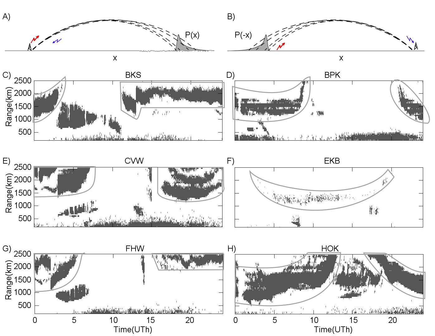
Figure 2: A) - formation of GS signal; B) - formation of noise power level by distribution of noise sources. Red and blue arrows in A-B) mark transmitted and received signals; C-H) - the position of the signals, defined by FitACF algorithm as GS, during 18/04/2016 on the radars BKS, BPK, CVW, EKB, FHW, HOK. Gray enclosed areas correspond to GS when focusing in the F-layer. Other areas are defined by the algorithm, as GS, but having, sometimes, an ionospheric origin.

In this study, the position of the F-layer GS signal was solved for each radar beam separately and independently. To generate input data for the GS positioning algorithm for each moment we identify the ranges where the signals have the maximum amplitude in the radar data. For this purpose we select only signals determined by the standard FitACF algorithm to be GS signal.

Using these prepared input data, we determine the smooth curve of the distribution of GS with range, within the framework of an empirical ionospheric model with a small number of parameters, adapted to the experimental data. The problem of determining the position of the GS signal causes certain difficulties connected to the presence of a large number of possible focusing points associated with the heterogeneity of the ionosphere along the signal propagation path Stocker . (2000) and ionospheric scattered signals incorrectly identified as GS signals.

For an approximate single-valued solution of this problem, we reformulate the problem as the problem of producing a GS signal in a plane-layered ionosphere with a parabolic layer with parameters estimated from the GS signal. In the framework of the plane-layered ionosphere with a parabolic F-layer, we have the following expression for the radar range to the boundary of the dead zone Chernov (1971):

$$R_{model}=\frac{f_{0}}{f_{oF2}}\left\{2h_{mF2}\sqrt{\chi}+\Delta h\cdot ln\left(\frac{1+\sqrt{\chi}}{1-\sqrt{\chi}}\right)\right\}$$ (3)

where $\chi=\frac{h_{mF2}-\Delta h}{h_{mF2}}$; $h_{min}=h_{mF2}-\Delta h$ - is the minimal height of the ionosphere, obtained from the condition $N_{e}(h_{min})=0$; $h_{mF2}$ is the height of the electron density maximum in the ionosphere, obtained from the condition $N_{e}(h_{mF2})=max$; $f_{oF2}$ is the plasma frequency of the F2 layer; $f_{0}$ is the carrier frequency of the sounding signal.

In this model, the geometric distance $D$ over the Earth surface to the point of focusing is defined as Chernov (1971):

$$D_{model}=R_{model}cos(\Theta_{model})$$ (4)

The elevation angle $\Theta_{model}$ of the signal arriving from the dead zone boundary according to this model is calculated as:

$$cos(\Theta_{model})=\sqrt{1-\chi\left(\frac{f_{0}}{f_{oF2}}\right)^{-2}}$$ (5)

For interpretation of absorption the elevation angle is very important: in the model of the plane-layered ionosphere it also corresponds to the elevation angle in the D-layer, and relates the observed absorption to absorption of vertically propagating radio space signal. So, this angle is important for the interpretation of absorption, both in the case of observing GS Watanabe  Nishitani (2013); Chakraborty . (2018); Fiori . (2018) and in the case of minimal noise analysis Berngardt . (2018); Bland . (2018). Most of the radars do measure the elevation angle. However, since many antenna characteristics in the HF range vary with time it is very important to calibrate the angle. This should be performed on each radar separately and regularly Ponomarenko . (2015); Chisham (2018); Shepherd (2017) and requires significant computations. To simplify the problem of smooth and continuous calculation of the GS elevation, we decided to use model calculations of the angle based on propagation in the adapted ionosphere model. In this sense this method is close to the approach used in Ponomarenko . (2015). One needs to just choose a proper ionospheric model.

The reference ionospheric model IRI Bilitza . (2017) is a median model and sufficiently smooth in time, but by default it does not correctly describe fast changes of $foF2$ in some situations, especially at high latitudes Blagoveshchenskii . (2015). This problem becomes especially critical for GS signal range calculations for sunset and sunrise periods. Searching for one or several IRI parameters that are constant during the day will not solve the problem, so it is necessary to use either an adaptive model that more adequately describes these periods, or to use IRI model corrected for each moment using data from an ionosonde network Galkin . (2012); Blagoveshchenskii . (2015). We use an adaptive model, which is easier to implement and does not require additional data and instruments.

The adaptive model of the parabolic-layer ionosphere was used with a nonlinear model for $foF2(t)$ and constant values for $h_{mF2}$ and $\Delta h$:

$$f_{oF2}(t)=f_{oF2,min}+\left(f_{oF2,max}-f_{oF2,min}\right)\varepsilon(t)$$ (6)

$$\varepsilon(t)=\frac{atan\left(\beta\cdot\left(\Theta(t-\Delta T)-\alpha\right)\right)-atan\left(\beta\cdot\left(\Theta_{min}-\alpha\right)\right)}{atan\left(\beta\cdot\left(\Theta_{max}-\alpha\right)\right)-atan\left(\beta\cdot\left(\Theta_{min}-\alpha\right)\right)}$$ (7)

where $\Theta(t)$ is the cosine of the solar zenith angle at the radar location as a function of the time $t$; $\Theta_{min},\Theta_{max}$ is the maximal and minimal cosine of the solar zenith angle during the day; $\alpha,\beta,\Delta T$ are modeled parameters, computed during the fitting procedure. More correctly solar zenith angle should be calculated at the point of radiowave absorption but in this paper we do not use this. The parameter $\Delta T$ compensates the difference in the first approximation.

The required strong nonlinearity of the model during sunset and sunrise moments is provided by the $atan()$ function, by the cosine of the solar zenith angle $\Theta(t)$ and controlled by several parameters: $\alpha,\beta,\Delta T,f_{oF2,max},f_{oF2,min}$. The model has enough degrees of freedom to describe the fast dynamics of $f_{oF2}(t)$ during solar terminator transitions. Taking into account the diurnal variation of $h_{max},\Delta h$ does not significantly improve the model, since these changes can be compensated by changes in the $f_{oF2}$ parameter.

The use of the cosine of solar zenith angle $\Theta(t)$ and the small time delay $\Delta T$ allows us describing the GS dynamics during sunrise and sunset more accurately and including the geographic position of the radar into the model. The choice of normalization in (7) is made so that $\varepsilon(t)$ takes values in the range [0,1] during the day. Therefore $\varepsilon(t)$ reaches its maximal value near noon and its minimal value near midnight. As a result the model for $f_{oF2}(t)$ (6) also reaches its maximal value $f_{oF2,max}$ near noon and its minimal value $f_{oF2,min}$ - near midnight.

When searching for optimal parameters of the model (3), the constant height of the maximum $h_{mF2}$ and the half-thickness of the parabolic layer $\Delta h$ were assumed to be 350 km and 100 km, respectively. The variations allowed in the model are the following:

$$\left\{\begin{array}[]{l}f_{oF2,max}\in[1,33]MHz;\\ f_{oF2,min}\in[\frac{1}{16},\frac{7}{16}]\cdot f_{oF2,max}MHz;\\ \beta\in[1,5];\\ \alpha\in[-1,1];\\ \Delta T\in[0,3]hours\end{array}\right.$$ (8)

An important problem in approximating the experimental data is the fitting method. A feature of the GS signal is its asymmetric character (1): it has a shorter front at ranges below GS signal power maximum, and a longer rear at ranges above GS signal power maximum. Therefore, the distribution of errors in determining the GS signal can be asymmetric near the mean value. Because of this, the use of the standard least squares method, oriented to "white" symmetrical noise, can produce a regular error. The existence of ionospheric scattering and several propagation modes aggravates the situation even more and substantially increases the approximation errors.

To improve the accuracy of the approximation, a special fitting method has been developed to detect GS-signal smooth dynamics in the presence of signals not described by the GS model. The fitting method consists of three stages. At the first stage, the preliminary fitting of the model is made. This stage is required for preliminary rejection of ionospheric scattering and possible additional modes of propagation. At the second stage, we reject those signals, which differ significantly by range from the model. At the third stage, the final fitting of the model is made. During the first and third stages, a genetic algorithm is used Simon (2013), as a method of searching for an optimum, but with different input data and with different functionals of the optimum. At the second stage a kind of cluster analysis Bailey (1994) is used.

An illustration of the algorithm operation is shown in Fig.3A-F for 18/04/2016 experimental data. There is good correspondence between the model range and the regular dynamics of the power of the scattered signal, which indicates a generally good stability of the technique. Violet circles denote the points of the GS, extracted from the radar data and serve as input for the first algorithm stage. The blue crosses denote the points that passed the second stage (exclusion of ionospheric scattering). The black lines represent the model dynamics of the GS signal range calculated at the third stage. The line can be discontinuous due to changes of radar operational frequency or night propagation conditions. It can be seen from the figure that qualitatively the technique fits the GS radar range quite well.

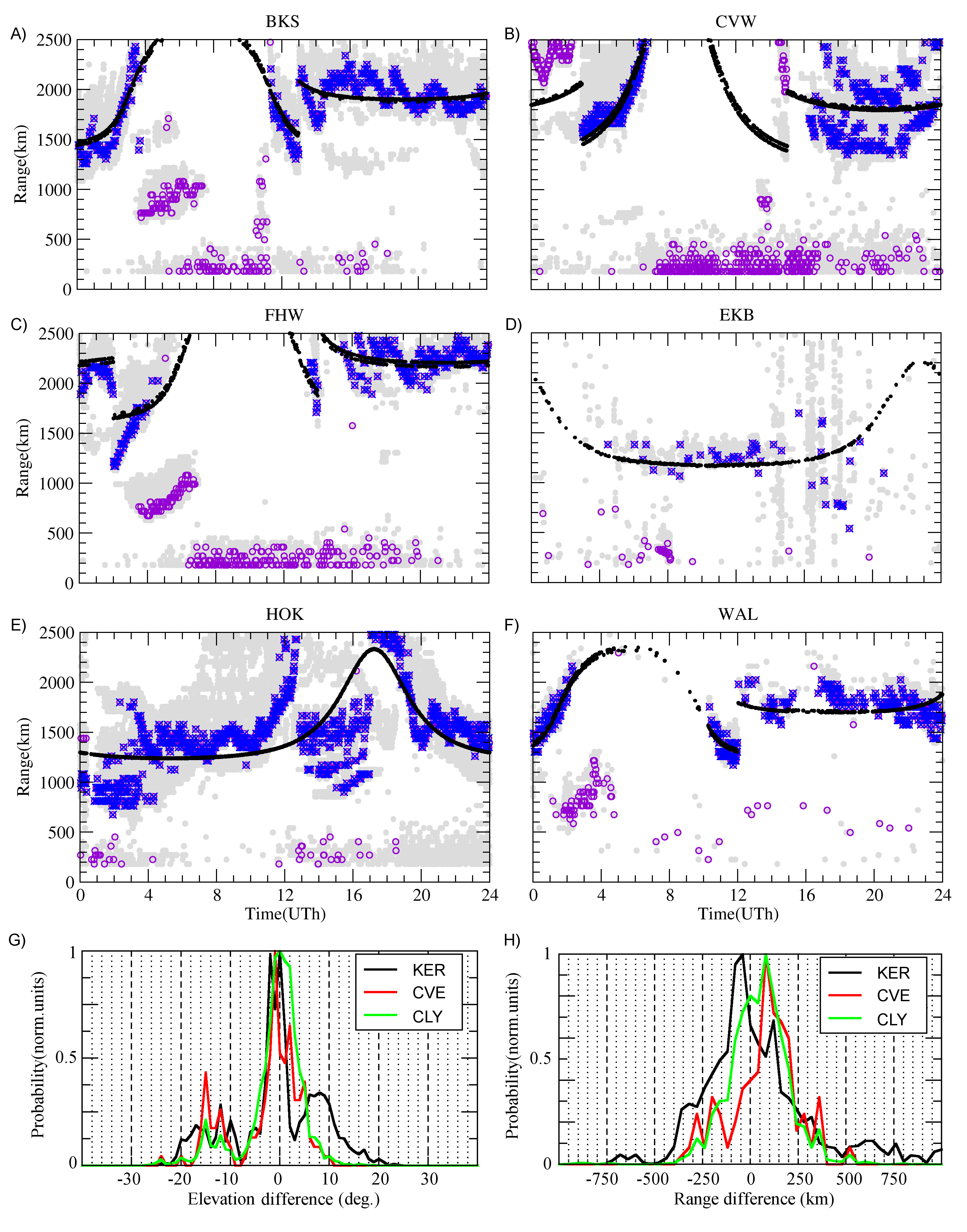
Figure 3: A-F) Illustration of the work of the fitting technique on various radars during 18/04/2016. Violet - non-GS data, detected at the second stage; blue - GS data, used for 3rd stage; black - GS distance, detected at 3rd stage. G) - the distribution of difference between model and measured GS elevation angles according to the KER, CVE and CLY radar data 18/04/2016. H) - the distribution of difference between model and measured GS range according to KER, CVE and CLY radar data 18/04/2016.

Let us describe the fitting stages in detail.

The points participating in the first stage fitting were determined by the following condition:

$$R_{exp}(Bm,t)=argmax_{R}(P(Bm,t,R):GSFLAG(Bm,t,R)=true)$$ (9)

where $Bm$ is the beam number, $t$ is the time, $GSFLAG$ is the GS attribute at the given range, calculated by the standard FitACF algorithm Ponomarenko  Waters (2006) . The selection rule (9) means that at each moment and on each beam a single point is found in which the power of the scattered signal is the maximal over all the signals defined as a GS at this moment and this beam. Thus, at each moment and for each beam, not more than a single point is selected, which is used later for fitting. A complete set of points participating in the fitting on a single beam is shown in Fig.3A-F by violet circles.

At the first stage, the fitting of the model (3,6,8) is made over these selected points (this corresponds to 24 hours of measurements at a single beam). In order to reduce the error in the presence of ionospheric scatter and additional modes, we used the following optimizing condition for the fitting:

$$\Omega(Bm)=\sum_{i=0}^{N}W(\delta R_{exp,i})=max$$ (10)

where $N$ is the total number of selected points (9) in the data involved in the fitting, and $W(\delta R_{exp,i})$ is the weight function. The maximization function (10) and the determination of the ionospheric parameters are carried out separately for each beam $Bm$. We do not require these model parameters to be close to each other on different beams. Our aim is to get smooth and physically reasonable radar distances and elevation angles. Their correctness will be discussed later.

The difference $\delta R_{exp,i}$ of the experimental range from the model range is defined as:

$$\delta R_{exp,i}=R_{model,i}-R_{exp,i}$$ (11)

Due to the asymmetric structure of GS signal over range, an asymmetric weight function $W$ was chosen:

$$W(\delta R_{exp})=\left\{\begin{array}[]{l}e^{-\frac{\delta R_{exp}}{200[km]}};\delta R_{exp}\geq 0\\ e^{\frac{\delta R_{exp}}{20[km]}};\delta R_{exp}<0\end{array}\right.$$ (12)

This function $W$ takes its maximal value when the experimental data coincide with the model data ($\delta R_{exp}=0$), and falls to zero if they differ too much ($|\delta R_{exp}|\rightarrow\infty$).

The choice of characteristic scales of 20 and 200 km is related to the characteristic durations of the edges of the GS signal. It is obvious that using such a weight in white noise conditions give a biased estimate - the model curve passes on average not in the middle of the experimental points set, but closer to its lower boundary, approximately with the ratio 1:10. However, in this problem the result corresponds well to the physical meaning and structure of the GS signal: its maximal power position is shifted to smaller distance, so this should qualitatively compensate the ’non-whiteness’ of the observed GS range variations. It should set the model of GS range closer to reality than the range calculated by the standard least-squares method. On the other hand, the use of such a weight function makes it possible to minimize the contribution of points substantially away from the model track (these are ionospheric scatter and other propagational modes) and to discard them from consideration during fitting.

As shown by qualitative analysis, the use of the weight function makes it possible to increase the stability of the technique in the presence of other modes and ionospheric scatter, and to carry out a model track near the lower boundary of the experimental GS data, which corresponds to the maximal energy of the GS signal.

The second stage of the algorithm is the rejection of ionospheric scattering and other propagation modes from the data. It is based on the cluster analysis technique, and close to the one used in Ribeiro . (2011). All the points are put into range-time grid of values (100x100). Thus the normalized range and moment of each point are scaled to integer values [0,100]. For all the combinations of such points (i.e. pairs), an Euclidean distance is calculated, and the points are divided into a clusters based on the distances between them. Every point in a single cluster has a nearest neighbor point in the same cluster at distance that does not exceed the doubled median distance calculated over the whole dataset. This allows us to separate the dataset into isolated clusters.

If the optimal model GS curve, calculated at the first stage, crosses a cluster at least at one point, the whole cluster is considered a GS signal. Otherwise the cluster is considered as not GS signal, and all the cluster points are excluded from subsequent consideration. The signals defined in the second stage as GS signals are shown by blue crosses in the Fig.3A-F, other signals are rejected at this stage and marked in the Fig.3A-F by violet circles.

In the third stage we believe that only F-layer GS signal points exist in the filtered data, and we can use the traditional least squares method to fit the model GS range function to the data:

$$\Omega(Bm)=\sum_{i=0}^{M}\delta R_{exp,i}^{2}=min$$ (13)

where $M$ is the number of GS points remaining after the second stage. The fitting of the modelled GS range at the third stage is shown in the Fig.3A-F by the black line.

In Fig.3A-F one can also see conditions for which the algorithm does not work well. This happens when ionospheric scattering appears at distances that are close to the daytime GS distance (Fig.3E, 00-03UT, 12-17UT; Fig.3F, 15-19UT). Since X-ray solar flares effects are observed mostly during the day Berngardt . (2018), the nighttime areas are not statistically important for this paper. So we do not pay attention to possible nighttime model range errors. A more critical problem is the case when the 1st and 2nd hop signals (Fig.3B, 17-24UT) are observed equally clearly and with nearly the same amplitude. So the model signal is forced to pass in the middle between these tracks. In this case, a significant regular error appears. Therefore, for a small amount of validated data, (Fig.3D), the algorithm can fail.

The model results have been compared with measurements made by the polar cap (CLY), sub-auroral (KER) and mid-latitude (CVE) radars on 18/04/2016. The root-mean-square error between the model elevation angle and the experimental measurements calculated from the interferometric data is $6-9^{o}$, with an average error of $1-3^{o}$ (Fig.3G). The root-mean-square error between the model GS range and the experimental measurements calculated for 18/04/2016 for these radars is 166-315 km , with an average error of 7-47 km (Fig.3H). The comparison shows that the technique can be used for processing polar cap, sub-auroral, and mid-latitude radar data.

In conlusion, in most cases, the algorithm works well enough to enable proper statistical conclusions. The smallness of the average range and elevation angle errors make it possible to use this technique for determining the model GS to carry out statistical studies on a large volume of experimental radar data.

Finally, to identify which hop produces most of the noise absorption, we analyzed the cases when the 1st hop and 2nd hop GS signal locations are at opposite sides of the solar terminator (i.e. in lit and unlit regions). We studied only cases when the noise absorption correlates well with X-rays at 1-8$\mathring{A}$. The 2nd hop GS distance was estimated by doubling the first hop GS distance (4). This allows us to estimate geographical location of 2nd hop GS region. Since the absorption correlating with X-rays is mainly associated with the lit area Berngardt . (2018), the studied cases allow us to statistically identify the (lit) hop of most effective absorption. For the $\approx 400$ cases found with the correlation coefficient $R>0.6$ the probability of the absorption at the 1st hop is $78\%$. For the $\approx 70$ cases found with $R>0.9$ the probability of absorption at the 1st hop is $95.5\%$.

We made a similar comparison of the point above the radar and the point near the edge of the GS region. Our analysis has shown that the probability of absorption near GS region for $R>0.8$ (over 15 cases) is $54\%$, for $R>0.85$ (over 10 cases) is $75\%$ , and for $R>0.9$ (over 4 cases) is $100\%$.

Therefore, in most situations, the daytime noise absorption can be interpreted as absorption on the 1st hop, with the most probable location near the dead zone.

3 Dependence of the absorption on the sounding frequency

Using the model of the GS signal range described above, it is possible to automatically estimate the elevation angle of the incoming noise signal and, thereby, to transform the oblique absorption to the vertical absorption. Knowing the height of the absorbing region and the range to GS, it is possible to estimate the geographical position of the absorbing region.

Another important factor that needs to be taken into account is the frequency dependence of the absorption. Using it one can interpolate the absorption measured at the radar operating frequency to the absorption at a fixed frequency. At present, several variants of absorption frequency dependence are used in the analysis of experimental data and forecasting. The DRAP2 model DRAP Documentation (2010); Akmaev, R. A. (2010) and some nowcast PCA models Rogers  Honary (2015) use a frequency dependence given by $A[dB]=A_{0}f^{-1.5}$, based on Sauer  Wilkinson (2008). A frequency dependence $A=A_{0}f^{-1.24}$ is proposed in Schumer (2010). From the theory of propagation of radio waves, the frequency dependence for sufficiently high probing frequencies exceeding the collision frequency $2\pi f\gg\nu$ absorption should have the dependence $A=A_{0}f^{-2}$ Davies (1969); Hunsucker  Hargreaves (2002). Computational models like Eccles . (2005); Pederick  Cervera (2014) use an ionospheric and a radio wave propagation model to calculate the absorption on each particular path and do not use an explicit frequency dependence.

To perform a comparative statistical analysis on a larger radar dataset, it is necessary to retrieve the experimental dependence of the absorption on the frequency of the radar. To determine this dependence, a correlation analysis of the absorption at various frequencies was carried out. We selected ’multi-frequency experiments’, that is, experiments for which, during 6 minutes, a certain radar simultaneously operated at least on 2 frequencies, separated by at least 10%, at the same azimuth. After selecting these experiments we built regression coefficients between the noise levels at different frequencies for each ’multi-frequency experiment’ , taking into account the possibility of different background noise levels and their various (linear) time dependencies. Thus, the regression coefficient $A_{0}$ for each ’multi-frequency experiment’ was determined as the value minimizing the root-mean-square deviation of noise attenuation $P_{1}(t),P_{2}(t)$ at frequencies $f_{1},f_{2}$ respectively. In other words, $A_{0}$ is defined as the solution to the problem:

$$\Omega=\int_{T_{flare}-1h}^{T_{flare}+2h}\left(P_{1}(t)[dB]-\left\{A_{0}P_{2}(t)[dB]+A_{1}+A_{2}t\right\}\right)^{2}dt=min$$ (14)

The integration was made over the regions $P_{1}(t)<0.9\cdot max(P_{1}),P_{2}(t)<0.9\cdot max(P_{2})$ to exclude noise saturation effects from consideration. To increase the validity of the retrieved data, we analyzed only the cases where the correlation coefficient between the noise attenuation and the variations of the intensity of solar radiation in the 1-8$\mathring{A}$ band exceeded 0.4, which indicates a statistically significant absorption effect Berngardt . (2018). As a result, we obtained a statistical distribution of the exponent of the power-law dependence of the absorption on the frequency

$$A[dB]\sim f^{-\alpha}$$ (15)

by calculating the ratio for every experiment:

$$\alpha_{i}=\frac{log(A_{0,i})}{log(f_{1,i}/f_{2,i})}$$ (16)

where $f_{2,i},f_{1,i}$ are the frequencies of noise observation simultaneously on the same beam at the same radar, and $A_{0,i}$ is the coefficient of regression between the absorption and X-ray flare dynamics at different sounding frequencies; $i$ is the experiment number.

Fig.4A shows the parameters of statistical distribution of $\alpha$ calculated over ’multi-frequency experiments’ for relatively high frequency difference ($f_{1}/f_{2}\in[1.2,1.3];f_{1}/f_{2}\in[1.3,1.5];f_{1}/f_{2}\in[1.5,1.6]$) and absorption for correlating ($|R|>0.4$) with 1-8$\mathring{A}$ solar radiation. To improve the estimates, we selected only experiments with small carrier frequency variations $\delta f_{1},\delta f_{2}$ during flare observations ($|\delta f_{1}|,|\delta f_{2}|<150kHz$) around the average sounding frequencies ($f_{1},f_{2}$). In other words, we investigated multi-frequency experiments with a large enough difference between two frequencies, that is, we required

$$|f_{1}-f_{2}|>3\cdot(|\delta f_{1}|+|\delta f_{2}|)$$ (17)

This final distribution corresponds to 1662 individual experiments at 18 different radars (BKS, BPK, CLY, DCE, EKB, GBR, HKW, HOK, INV, KAP, KOD, KSR, MCM, PGR, RKN, SAS, TIG, WAL). It can be seen from Figure 4 that the distribution of $\alpha$ has an average around 1.6 (for $f_{1}/f_{2}>1.3$) and RMS can reach about 0.3 (at $f_{1}/f_{2}>1.5$). The statistics indicate that the dependence of the absorption on the frequency in the range 8-20 MHz can be described more stably by the empirical dependence $A[dB]\sim f^{-1.6}$, which is close to $\alpha=1.5$, used in the conventional absorption forecast model DRAP2 DRAP Documentation (2010); Akmaev, R. A. (2010). Therefore, we will use the empirically found value $\alpha=1.6\pm 0.3$ in the following work.

4 Correlation of absorption dynamics with solar radiation of different wavelengths

The next important issue arising in the investigation of noise data by coherent radars is the interpretation of the detailed temporal dynamics of the noise absorption. As shown in Berngardt . (2018) and seen in fig.1A-C, the front of noise absorption at the radar correlates well with the shape of the X-ray flare according to GOES/XRS 1-8$\mathring{A}$. The rear is substantially delayed with respect to the X-ray 1-8$\mathring{A}$ flare. As the preliminary analysis showed, this is a relatively regular occurrence for the data from 2013 to 2017. Since the absorption from the rear is delayed for tens of minutes, it cannot be explained only in terms of recombination in the ionized region.

One possible explanation for the delay in the rear is the contribution to ionospheric absorption of regions higher than the D layer, ionized by solar radiation lines other than the X-ray 1-8 $\mathring{A}$. It is known that the lower part of the ionosphere (layers D- and E-) is ionized by wavelengths <100 $\mathring{A}$ Banks  Kockarts (1973) as well as by Lyman-$\alpha$ line (about 1200$\mathring{A}$). Most often, researchers analyze the association of absorption with X-ray radiation 1-8 $\mathring{A}$ only, measured by GOES/XRS and associated with the ionization of the D-layer Rogers  Honary (2015); Warrington . (2016), see fig.1D. However, the absorption is important not only in the D-layer but also in the E-layer, the ionization of which is caused by other components of the solar radiation. In particular, soft X-ray 10-50 $\mathring{A}$ radiation is taken into account in modern D-layer ionization models Eccles . (2005) (where it is taken into account using a solar spectrum model) . The combined effect of increasing absorption in the E-layer and a slight refraction extending the path length in the absorbing layer leads to the need to take into account the ionization of the E-layer.

To analyze the correlation of the noise attenuation with various solar radiation lines, we carried out a joint analysis of the absorption during the 80 flares of 2013-2017 and data from varied instruments, namely: GOES/XRS Hanser  Sellers (1996); Machol  Viereck (2016), GOES/EUVS Machol . (2016), SDO/AIA Lemen . (2012), PROBA2/LYRA Hochedez . (2006); Dominique . (2013), SOHO/SEM Didkovsky . (2006), SDO/EVE(ESP) Didkovsky . (2012). These instruments provide direct and regular observations of solar radiation in the wavelength range 1-2500$\mathring{A}$ during the period under study (see Table 2 for details). It is well known that at different wavelengths the solar radiation dynamics during flares is different Donnelly (1976). This allows us to find the solar radiation lines that most strongly influence the dynamics of the noise variations at the coherent radars.

To determine the effective ionization lines, we calculate the following probability:

$$P\left({\Lambda}\right)=P\left(R(P(t),I_{\Lambda}(t))\geq R(P(t),I_{1-8\mathring{A}}(t))|R(P(t),I_{1-8\mathring{A}}(t))\geq 0.4\right)$$ (18)

In this expression, $P\left({\Lambda}\right)$ is the probability that the correlation coefficient $R(P(t),I_{\Lambda}(t))$ of the observed absorption $P(t)$ with the intensity $I_{\Lambda}(t)$ of a given solar radiation line $\Lambda$ during the X-ray flare period will not be lower than the correlation coefficient $R(P(t),I_{1-8\mathring{A}}(t))$ of the observed absorption $P(t)$ with the intensity $I_{1-8\mathring{A}}(t)$ of GOES/XRS 1-8$\mathring{A}$ line. The calculations are carried out only for cases during which the correlation coefficient between absorption and GOES/XRS solar radiation is greater than 0.4.

It should be noted that if the distribution of values of the correlation coefficients are similar and independent for different wavelengths of solar radiation, then $P(\Lambda)$ should not exceed 0.5. Exceeding this level indicates a line of solar radiation to be a controlling factor for the attenuation of the noise. Figure 4B shows the results of this analysis based on the processing of over 11977 individual observations.

One can see from Figure 4B that very often (in 62 to 68% of the cases) $P(\Lambda)$ exceeds 0.5 for $\Lambda$ in the ranges SDO/AIA 94$\mathring{A}$, SDO/EVE 1-70$\mathring{A}$, 300-340$\mathring{A}$, SDO/AIA 304,335$\mathring{A}$, SOHO/SEM 1-500$\mathring{A}$. This indicates the need to take these solar radiation lines into account when interpolating the HF noise attenuation. All these lines are absorbed below 150 km (Tobiska ., 2008, fig.2). They are therefore sources of ionization in the lower part of the ionosphere and are contributing to the radio noise absorption observed in the experiment.

Let us demonstrate the potential of using the linear combination of six lines from these spectral ranges (1-8$\mathring{A}$, 94$\mathring{A}$, 304$\mathring{A}$, 335$\mathring{A}$, 1-70$\mathring{A}$, 1-500$\mathring{A}$) instead of just single 1-8$\mathring{A}$ GOES/XRS line. Let us assume that ionization is produced by different lines independently, the contributions of each line to ionization are positive, and are retrievable. To search for the amplitude of these contributions , we used the non-negative least-squares method Lawson  Hanson (1995). It provides an iterative search for the best approximation of experimental noise attenuation $P_{att}(t)$ by a linear combination of solar radiation dynamics at different wavelengths ($P_{1-8\mathring{A}}(t)$, $P_{94\mathring{A}}(t)$, $P_{304\mathring{A}}(t)$, $P_{335\mathring{A}}(t)$, $P_{1-70\mathring{A}}(t)$, $P_{1-500\mathring{A}}(t)$) with unknown nonnegative weighting multipliers. In addition we also take into account slow background noise dynamics by adding a linear dependence $C_{0}+C_{1}t$ into the regression.

Finally, we search for parameters $C_{0..7}$ that solve the problem:

$$\int_{T_{flare}-1h}^{T_{flare}+2h}(P_{att}(t)-C_{0}-C_{1}t-C_{2}P_{1-8\mathring{A}}(t)-C_{3}P_{94\mathring{A}}(t)-C_{4}P_{304\mathring{A}}(t)$$ (19)

$$-C_{5}P_{335\mathring{A}}(t)-C_{6}P_{1-70\mathring{A}}(t)-C_{7}P_{1-500\mathring{A}}(t))^{2}dt=min$$ (20)

under the limitation that $C_{2},C_{3},C_{4},C_{5},C_{6},C_{7}$ be all positive.

Examples of approximations and statistical results are shown in Fig.4C-F. It can be seen that the sum of four lines (dot-dashed green line) approximates the experimental data much better than just a single GOES/XRS (dotted black line) solar radiation line. Fig.4C shows the distribution of the correlation coefficients when the experimental data are approximated by linear combinations of the lines 1-8$\mathring{A}$, 94$\mathring{A}$, 304$\mathring{A}$, 335$\mathring{A}$, 1-70$\mathring{A}$, and 1-500$\mathring{A}$ . The figure shows that the combination of the lines 1-8$\mathring{A}$ and 94$\mathring{A}$ (solid black line) fits the experimental data no worse than the combination of all six lines (dot-dashed green line), and significantly better than the single line 1-8$\mathring{A}$ (dotted black line). This allows us to use a combination of the two lines 1-8$\mathring{A}$ and 94$\mathring{A}$ as parameters of the noise attenuation model during X-ray solar flares at these radars.

In this paper we analyze only X-ray flares, and the level of Lyman-$\alpha$ line is comparatively weak. Therefore the well-known dependence of the D-layer ionization with Lyman-$\alpha$ is not detected (see Fig.4B).

Lines 10-100$\mathring{A}$ are usually absorbed at heights of the order of and below 100 km (Banks  Kockarts, 1973, fig.1.7, par.6.3.), This indicates a significant contribution of the lower part of the E-layer to the noise absorption observed by the radars.

The median value of the correlation coefficient of the noise attenuation with 1-8$\mathring{A}$ is 0.62, with the combination of 1-8$\mathring{A}$ + 94$\mathring{A}$ lines is 0.76, and with the combination of all 6 lines is 0.73.

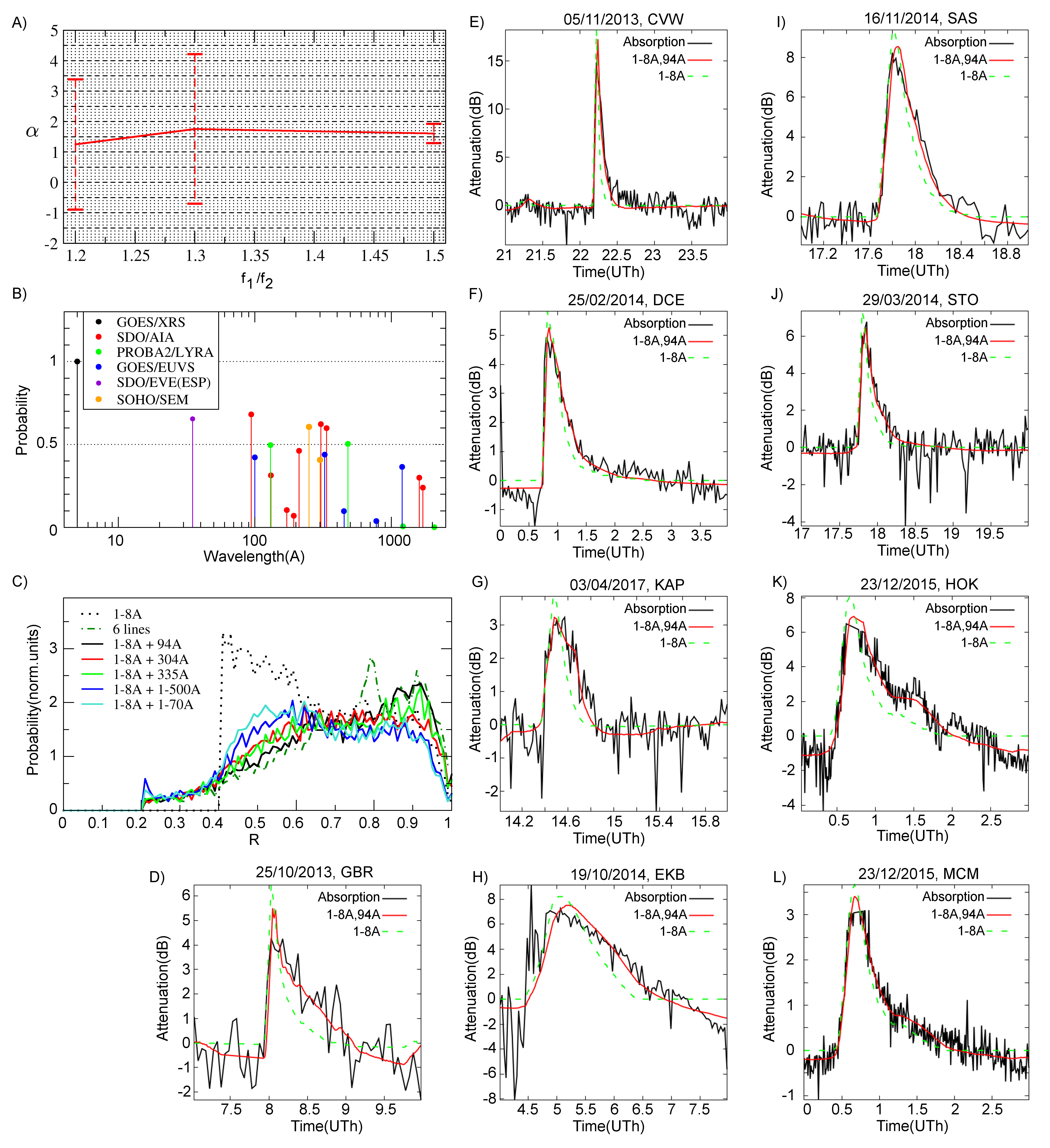
Figure 4: A) Average and RMS of the power-law (15) coefficient $\alpha$ of the absorption frequency dependence as a function of relation of frequencies during multi-frequency experiments; B) The probability $P\left({\Lambda}\right)$ (18) over all the flares and the radars; C) Distribution of correlation coefficients for various approximations of the noise absorption experimental data; D-L) are examples of fitting the attenuation of HF noise by different combinations of solar spectrum lines (at different radars during different X-ray flares).

Thus, taking into account the line 94$\mathring{A}$ leads to an increase in the median correlation coefficient from 0.62 to 0.76, while adding other lines does not significantly increase the correlation. This allows us concluding that use of the 1-8$\mathring{A}$ and 94$\mathring{A}$ solar radiation lines as a proxy of the noise attenuation profile potentially allows a more accurate approximation of the temporal dynamics of the experimentally observed noise attenuation, and as a result, of the temporal dynamics of the absorption of the HF radio signals in the lower part of the ionosphere. Fig.4D-L shows the attenuation of HF noise dynamics when it is approximated only by GOES/XRS 1-8$\mathring{A}$ (green dashed line) and by a combination of GOES/XRS 1-8$\mathring{A}$ and SDO/AIA 94$\mathring{A}$ solar radiation (red line). The approximations are shown for several radars during several flares. It can be seen from the figure that taking into account intensity of the SDO/AIA 94$\mathring{A}$ line significantly improve the accuracy of fitting the noise attenuation dynamics. Therefore it is necessary to take into account not only the D-layer, but also the E-layer of the ionosphere for the interpretation of the noise absorption during X-ray solar flares. This corresponds well with the results obtained by Eccles . (2005).

5 Diagnostics of global absorption effects

Taking into account all of the above, it is possible to build an automatic system suitable for global analysis of ionospheric absorption of HF radio waves over the area covered by radar field-of-views. The algorithm for constructing the automatic absorption analysis system consists of the following stages.

At the first stage, the GS signal range curve is determined from the daily behavior of the GS signal. We model the ionosphere as a parabolic layer of known half-thickness $\Delta h$ and height $h_{mF2}$, but of unknown amplitude $f_{oF2}(t)$ and dynamics. The temporal dynamics of $f_{oF2}(t)$ is approximated by the nonlinear parametric function (6), and its parameters are calculated from experimental data via a fitting procedure.

Using this GS signal range curve, the elevation angle of the received GS signal is estimated as a function of time. The location of the region making the main contribution to the absorption of the radio noise is found simultaneously. Its calculation is based on the Breit-Tuve principle Davies (1969) and on the assumption that the signal is reflected at the virtual height $h_{mF2}$. Such a calculation is carried out separately for each radar, for each beam. The algorithm for constructing the dynamics of GS range and the elevation angle is given above (3,5).

At the second stage, the noise absorption level $\widetilde{P}_{vert,10MHz}(t,\phi(t),\lambda(t))$ is estimated for the vertical radio wave propagation in the absorbing layer at a frequency of 10MHz for each beam of the radar, at a geographical point $(\phi(t),\lambda(t))$ corresponding to the position of the effective absorbing region. It is calculated from the noise variations $\widetilde{P}(t)$ detected by the radar, taking into account the elevation angle $\Theta_{model}$ of the radio signal propagation in the absorbing layer, which was calculated at the first stage. The absorption corresponds to the geographic coordinates $(\phi(t),\lambda(t))$, also calculated in the first stage, and set to the point which is farthest away from the radar (the trajectory crosses D-layer at two points). The observed dependence of absorption on frequency $f(t)$ is interpolated to 10MHz frequency using our retrieved median frequency dependence. The resulting expression for the vertical absorption is:

$$\widetilde{P}_{vert,10MHz}(t,\phi(t),\lambda(t))=\widetilde{P}(t)sin(\Theta_{model}(t))\left(\frac{f(t)}{f_{0}}\right)^{1.6}$$ (21)

where $f_{0}=10$MHz, and $f(t)$ is the radar sounding frequency.

Fig.5A-H shows the absorption dynamics over the radars field-of-views during the 07/01/2014 solar flare based on the proposed algorithm. One can see the global-scale absorption effect between 18:18 UT and 19:12 UT that corresponds to the solar X-ray flare. Each radar produces several measurement points, corresponding to the number of beams, one beam - one measurement point.

So the spatial resolution and resolved areas depend on radiowave propagation characteristics and could vary from flare to flare. For future practical purposes one can fit the obtained absorption measurements over space by a smoothing function or join them with regular riometric measurements.

One of the ways to smooth the obtained data is through their accumulation over latitude or longitude. It allows us to more clearly distinguish the temporal dynamics of absorption and to reveal its average latitudinal or longitudinal dependencies.

Fig.5I shows the dynamics of median absorption as a function of latitude during this event. The median was calculated over 3 geographical degrees. Fig.5J shows the dynamics of median absorption as a function of longitude during this event. The median was calculated over 3 geographical degrees. For comparison solar radiation at 1-8$\mathring{A}$ and 94$\mathring{A}$ is shown in Fig.5K. It can be seen from the figure that the proposed method makes it possible to investigate the spatio-temporal dynamics of absorption over a significant part of the Earth’s surface.

A joint analysis of Fig.5A-J allows, for example, to distinguish absorption regions in the lit area that correlate well with the flare (green regions) from the effects in the unlit area that can not be correctly interpreted with the approach taken in this paper. The system that we have constructed can be used for studies of spatio-temporal features of daytime absorption both as a separate network and with other instruments and techniques.

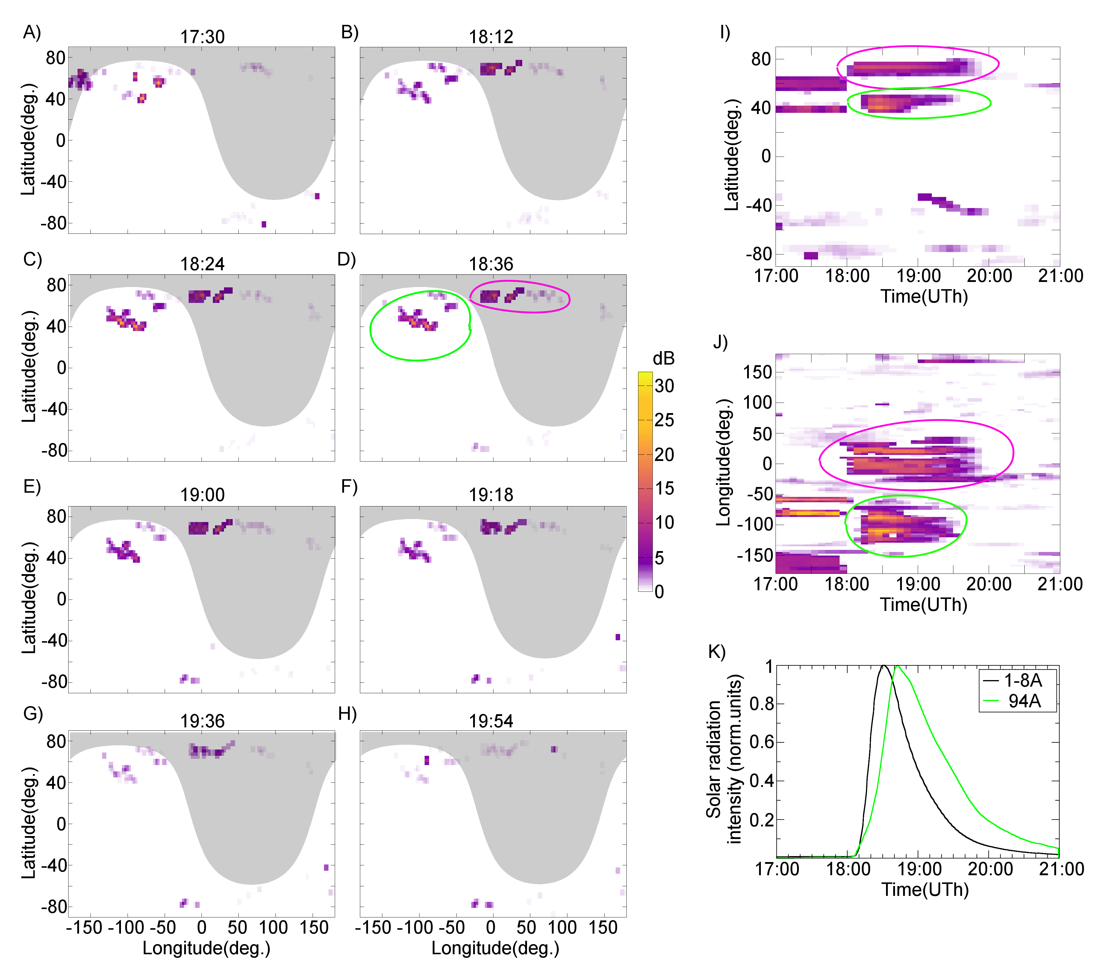
Figure 5: A-H) - vertical absorption dynamics at 10MHz during solar X-ray flare X1.2 07/01/2014 according to the radar network and model (21). Grey region marks unlit area at 100km height. I) - latitude absorption dynamics during the flare, median over all the longitudes; J) - longitude absorption dynamics during the flare, median over all the latitudes; K) the intensity of solar radiation from the data of GOES/XRS 1-8$\mathring{A}$ and SDO/AIA 94$\mathring{A}$. Color scale is the same for the figures A-J). Green and violet regions mark effects in lit and unlit conditions.

6 Conclusion

In the present work, a joint analysis was carried out of the data of 35 HF over-the-horizon radars (34 SuperDARN radars and the EKB ISTP SB RAS radar) during 80 solar flares of 2013-2017. The analysis shows the following features of the absorption of 8-20MHz radio noise.

The position of an effective noise source on the ground and the error in determining its location can be determined by the position of spatial focusing at the boundary of the dead zone and the form of this focusing (ground scatter signal). This allows using the GS signal to estimate the position of the region that makes the main contribution to the observed absorption of the HF radio noise at a particular radar frequency.

The analysis of the correlation between different solar radiation lines and HF noise dynamics has shown that the temporal variation of the absorption is well described by a linear combination of the solar radiation intensity at the wavelengths 1-8$\mathring{A}$ measured by GOES/XRS and at the wavelength of 94$\mathring{A}$ measured by SDO/AIA. This allows us to conclude that the main absorption is caused by ionospheric D and E layers. The assumption we used in our paper about a linear superposition of the contributions of each solar line to absoprtion is relatively rough. To solve more accurately for the reconstruction of the electron density profile from the experimentally observed noise absorption and from the solar spectrum, it is necessary to take into account the processes of ionization by the various radiation components and corresponding delays more correctly, for example, following the approach of Eccles . (2005).

The frequency dependence of the HF absorption is determined by the median dependence $A[dB]\sim f^{-1.6\pm 0.3}$.

A model and algorithms are constructed (21), that provides automatic radar estimates of vertical daytime absorption at 10 MHz. Using these model algorithms, it is possible to make statistical analysis and case-studies of the spatio-temporal dynamics of the absorption of HF radio waves globally, within the coverage area of radar field-of-views. Each radar produces several measurement points, corresponding to the number of beams, one beam - one measurement point. So the spatial resolution and resolved areas depend on radiowave propagation characteristics and will vary from flare to flare.

One important problem with the algorithm constructed here is the determination of the geographical location of the absorption region during the day. This location depends on whether the most intense 1-hop absorption is located near the radar or near the GS distance of the first hop. A similar problem arises with the URSI A1 method. For future applications, one might want to fit the retrieved absorption measurements through the use of a smoothing function over space. However, at night or near the terminator, this algorithm should not be used.

Another problem of the algorithm is the impossibility of taking into account irregular variations in the background ionosphere. This is important for a more correct estimation of ray trajectory and, as result, for more accurate estimation of the vertical absorption from the experimental data for specific observations. The use of calibrated experimental mesurements of the ray elevation angles of GS signals and new techniques for identifying GS signals from radar data should help to solve this problem in the future.

References

- Akmaev, R. A. (\APACyear2010) \APACinsertmetastarDRAP2{APACrefauthors}Akmaev, R. A. \APACrefYearMonthDay2010. \APACrefbtitleDRAP Model Validation: I.Scientific Report. DRAP Model Validation: I.Scientific Report. {APACrefURL} https://www.ngdc.noaa.gov/stp/drap/DRAP-V-Report1.pdf \PrintBackRefs\CurrentBib
- Bailey (\APACyear1994) \APACinsertmetastarbailey1994{APACrefauthors}Bailey, K. \APACrefYear1994. \APACrefbtitleTypologies and Taxonomies: An Introduction to Classification Techniques Typologies and Taxonomies: An Introduction to Classification Techniques (\BNUM 102). \APACaddressPublisherSAGE Publications. \PrintBackRefs\CurrentBib
- J. Baker \BOthers. (\APACyear2007) \APACinsertmetastarBaker_2007{APACrefauthors}Baker, J., Greenwald, R., Ruohoniemi, J., Oksavik, K., Gjerloev, J\BPBIW., Paxton, L\BPBIJ.\BCBL \BBA Hairston, M. \APACrefYearMonthDay2007. \BBOQ\APACrefatitleObservations of ionospheric convection from the Wallops SuperDARN radar at middle latitudes Observations of ionospheric convection from the Wallops SuperDARN radar at middle latitudes.\BBCQ \APACjournalVolNumPagesJournal of Geophysical Research (Space Physics)112A01303. {APACrefDOI} \doi10.1029/2006ja011982 \PrintBackRefs\CurrentBib
- K\BPBIB. Baker \BOthers. (\APACyear1988) \APACinsertmetastarBaker_1988{APACrefauthors}Baker, K\BPBIB., Greenwald, R., Villian, J\BPBIP.\BCBL \BBA Wing, S. \APACrefYearMonthDay1988. \APACrefbtitleSpectral Characteristics of High Frequency (HF) Backscatter for High Latitude Ionospheric Irregularities: Preliminary Analysis of Statistical Properties Spectral Characteristics of High Frequency (HF) Backscatter for High Latitude Ionospheric Irregularities: Preliminary Analysis of Statistical Properties \APACbVolEdTR\BTR \BNUM ADA202998. \APACaddressInstitutionJohns Hopkins Univ Laurel Md Applied Physics Lab. \PrintBackRefs\CurrentBib
- Banks \BBA Kockarts (\APACyear1973) \APACinsertmetastarbanks1973aeronomy{APACrefauthors}Banks, P.\BCBT \BBA Kockarts, G. \APACrefYear1973. \APACrefbtitleAeronomy Aeronomy (\BVOL A). \APACaddressPublisherAcademic Press, New York and London. \PrintBackRefs\CurrentBib
- Barthes \BOthers. (\APACyear1998) \APACinsertmetastarBarthes_1998{APACrefauthors}Barthes, L., Andre, D., Cerisier, J\BPBIC.\BCBL \BBA Villain, J\BHBIP. \APACrefYearMonthDay1998. \BBOQ\APACrefatitleSeparation of multiple echoes using a high–resolution spectral analysis for SuperDARN HF radars Separation of multiple echoes using a high–resolution spectral analysis for SuperDARN HF radars.\BBCQ \APACjournalVolNumPagesRadio Science3341005–1017. {APACrefDOI} \doi10.1029/98rs00714 \PrintBackRefs\CurrentBib
- Berngardt \BOthers. (\APACyear2018) \APACinsertmetastarBERNGARDT_20181{APACrefauthors}Berngardt, O\BPBII., Ruohoniemi, J\BPBIM., Nishitani, N., Shepherd, S\BPBIG., Bristow, W\BPBIA.\BCBL \BBA Miller, E\BPBIS. \APACrefYearMonthDay2018. \BBOQ\APACrefatitleAttenuation of decameter wavelength sky noise during x–ray solar flares in 2013–2017 based on the observations of midlatitude HF radars Attenuation of decameter wavelength sky noise during x–ray solar flares in 2013–2017 based on the observations of midlatitude HF radars.\BBCQ \APACjournalVolNumPagesJournal of Atmospheric and Solar-Terrestrial Physics1731 - 13. {APACrefDOI} \doi10.1016/j.jastp.2018.03.022 \PrintBackRefs\CurrentBib
- Berngardt \BOthers. (\APACyear2015) \APACinsertmetastarBerngardt_2015{APACrefauthors}Berngardt, O\BPBII., Zolotukhina, N\BPBIA.\BCBL \BBA Oinats, A\BPBIV. \APACrefYearMonthDay2015. \BBOQ\APACrefatitleObservations of field–aligned ionospheric irregularities during quiet and disturbed conditions with EKB radar: first results Observations of field–aligned ionospheric irregularities during quiet and disturbed conditions with EKB radar: first results.\BBCQ \APACjournalVolNumPagesEarth, Planets and Space671143. {APACrefDOI} \doi10.1186/s40623-015-0302-3 \PrintBackRefs\CurrentBib
- Bilitza \BOthers. (\APACyear2017) \APACinsertmetastarBilitza_2017{APACrefauthors}Bilitza, D., Altadill, D., Truhlik, V., Shubin, V., Galkin, I\BPBIA., Reinisch, B\BPBIW.\BCBL \BBA Huang, X. \APACrefYearMonthDay2017. \BBOQ\APACrefatitleInternational Reference Ionosphere 2016: from ionospheric climate to real–time weather predictions International Reference Ionosphere 2016: from ionospheric climate to real–time weather predictions.\BBCQ \APACjournalVolNumPagesSpace Weather418–429. \APACrefnote2016SW001593 {APACrefDOI} \doi10.1002/2016sw001593 \PrintBackRefs\CurrentBib
- Blagoveshchenskii \BOthers. (\APACyear2015) \APACinsertmetastarBlagov_2015{APACrefauthors}Blagoveshchenskii, D\BPBIV., Maltseva, O\BPBIA., Anishin, M\BPBIM., Rogov, D\BPBID.\BCBL \BBA Sergeeva, M\BPBIA. \APACrefYearMonthDay2015. \BBOQ\APACrefatitleModeling of HF propagation at high latitudes on the basis of IRI Modeling of HF propagation at high latitudes on the basis of IRI.\BBCQ \APACjournalVolNumPagesAdvances in Space Research573821-834. {APACrefDOI} \doi10.1016/j.asr.2015.11.029 \PrintBackRefs\CurrentBib
- Blanchard \BOthers. (\APACyear2009) \APACinsertmetastarBlanchard_2009{APACrefauthors}Blanchard, G\BPBIT., Sundeen, S.\BCBL \BBA Baker, K\BPBIB. \APACrefYearMonthDay2009. \BBOQ\APACrefatitleProbabilistic identification of high–frequency radar backscatter from the ground and ionosphere based on spectral characteristics Probabilistic identification of high–frequency radar backscatter from the ground and ionosphere based on spectral characteristics.\BBCQ \APACjournalVolNumPagesRadio Science445RS5012. {APACrefDOI} \doi10.1029/2009rs004141 \PrintBackRefs\CurrentBib
- Bland \BOthers. (\APACyear2018) \APACinsertmetastarBland_2018{APACrefauthors}Bland, E\BPBIC., Heino, E., Kosch, M\BPBIJ.\BCBL \BBA Partamies, N. \APACrefYearMonthDay2018. \BBOQ\APACrefatitleSuperDARN radar–derived HF radio attenuation during the September 2017 solar proton events SuperDARN radar–derived HF radio attenuation during the September 2017 solar proton events.\BBCQ \APACjournalVolNumPagesSpace Weather. {APACrefDOI} \doi10.1029/2018sw001916 \PrintBackRefs\CurrentBib
- Bliokh \BOthers. (\APACyear1988) \APACinsertmetastarBliokh1988{APACrefauthors}Bliokh, P\BPBIV., Galushko, V\BPBIG., Minakov, A\BPBIA.\BCBL \BBA Yampolski, Y\BPBIM. \APACrefYearMonthDay1988. \BBOQ\APACrefatitleField interference structure fluctuations near the boundary of the skip zone Field interference structure fluctuations near the boundary of the skip zone.\BBCQ \APACjournalVolNumPagesRadiophysics and Quantum Electronics316480–487. {APACrefDOI} \doi10.1007/bf01044650 \PrintBackRefs\CurrentBib
- Chakraborty \BOthers. (\APACyear2018) \APACinsertmetastarChakraborty_2018{APACrefauthors}Chakraborty, S., Ruohoniemi, J\BPBIM., Baker, J\BPBIB\BPBIH.\BCBL \BBA Nishitani, N. \APACrefYearMonthDay2018. \BBOQ\APACrefatitleCharacterization of Short–Wave Fadeout Seen in Daytime SuperDARN Ground Scatter Observations Characterization of Short–Wave Fadeout Seen in Daytime SuperDARN Ground Scatter Observations.\BBCQ \APACjournalVolNumPagesRadio Science534472-484. {APACrefDOI} \doi10.1002/2017RS006488 \PrintBackRefs\CurrentBib
- Chernov (\APACyear1971) \APACinsertmetastarChernov1971{APACrefauthors}Chernov, Y\BPBIA. \APACrefYear1971. \APACrefbtitleBackward–oblique sounding of the ionosphere(in russian) Backward–oblique sounding of the ionosphere(in russian). \APACaddressPublisherMoscow,Svyaz. \PrintBackRefs\CurrentBib
- Chisham (\APACyear2018) \APACinsertmetastarChisham_2018{APACrefauthors}Chisham, G. \APACrefYearMonthDay2018. \BBOQ\APACrefatitleCalibrating SuperDARN Interferometers Using Meteor Backscatter Calibrating SuperDARN Interferometers Using Meteor Backscatter.\BBCQ \APACjournalVolNumPagesRadio Science536761-774. {APACrefDOI} \doi10.1029/2017RS006492 \PrintBackRefs\CurrentBib
- Chisham \BOthers. (\APACyear2007) \APACinsertmetastarChisham_2007{APACrefauthors}Chisham, G., Lester, M., Milan, S., Freeman, M., Bristow, W., McWilliams, K.\BDBLWalker, A. \APACrefYearMonthDay2007. \BBOQ\APACrefatitleA decade of the Super Dual Auroral Radar Network (SuperDARN): scientific achievements, new techniques and future directions A decade of the Super Dual Auroral Radar Network (SuperDARN): scientific achievements, new techniques and future directions.\BBCQ \APACjournalVolNumPagesSurveys in Geophysics2833-109. {APACrefDOI} \doi10.1007/s10712-007-9017-8 \PrintBackRefs\CurrentBib
- Davies (\APACyear1969) \APACinsertmetastarDavies_1969{APACrefauthors}Davies, K. \APACrefYear1969. \APACrefbtitleIonospheric radio waves Ionospheric radio waves. \APACaddressPublisherBlaisdell Pub. Co. \PrintBackRefs\CurrentBib
- Detrick \BBA Rosenberg (\APACyear1990) \APACinsertmetastarDetrick_1990{APACrefauthors}Detrick, D\BPBIL.\BCBT \BBA Rosenberg, T\BPBIJ. \APACrefYearMonthDay1990. \BBOQ\APACrefatitleA phased–array radiowave imager for studies of cosmic noise absorption A phased–array radiowave imager for studies of cosmic noise absorption.\BBCQ \APACjournalVolNumPagesRadio Science254325-338. {APACrefDOI} \doi10.1029/RS025i004p00325 \PrintBackRefs\CurrentBib
- Didkovsky \BOthers. (\APACyear2012) \APACinsertmetastarDidkovsky_2012{APACrefauthors}Didkovsky, L\BPBIV., Judge, D., Wieman, S., Woods, T.\BCBL \BBA Jones, A. \APACrefYearMonthDay2012. \BBOQ\APACrefatitleEUV SpectroPhotometer (ESP) in Extreme Ultraviolet Variability Experiment (EVE): Algorithms and Calibrations EUV SpectroPhotometer (ESP) in Extreme Ultraviolet Variability Experiment (EVE): Algorithms and Calibrations.\BBCQ \APACjournalVolNumPagesSolar Physics2751179–205. {APACrefDOI} \doi10.1007/s11207-009-9485-8 \PrintBackRefs\CurrentBib
- Didkovsky \BOthers. (\APACyear2006) \APACinsertmetastarDidkovsky_2006{APACrefauthors}Didkovsky, L\BPBIV., Judge, D\BPBIL., Jones, A\BPBIR., Wieman, S., Tsurutani, B\BPBIT.\BCBL \BBA McMullin, D. \APACrefYearMonthDay2006. \BBOQ\APACrefatitleCorrection of SOHO CELIAS/SEM EUV measurements saturated by extreme solar flare events Correction of SOHO CELIAS/SEM EUV measurements saturated by extreme solar flare events.\BBCQ \APACjournalVolNumPagesAstronomische Nachrichten328136-40. {APACrefDOI} \doi10.1002/asna.200610667 \PrintBackRefs\CurrentBib
- Dominique \BOthers. (\APACyear2013) \APACinsertmetastarDominique_2013{APACrefauthors}Dominique, M., Hochedez, J\BHBIF., Schmutz, W., Dammasch, I\BPBIE., Shapiro, A\BPBII., Kretzschmar, M.\BDBLBenMoussa, A. \APACrefYearMonthDay2013. \BBOQ\APACrefatitleThe LYRA Instrument Onboard PROBA2: Description and In–Flight Performance The LYRA Instrument Onboard PROBA2: Description and In–Flight Performance.\BBCQ \APACjournalVolNumPagesSolar Physics286121–42. {APACrefDOI} \doi10.1007/s11207-013-0252-5 \PrintBackRefs\CurrentBib
- Donnelly (\APACyear1976) \APACinsertmetastarDonnelly_1976{APACrefauthors}Donnelly, R\BPBIF. \APACrefYearMonthDay1976. \BBOQ\APACrefatitleEmpirical models of solar flare X ray and EUV emission for use in studying their E and F region effects Empirical models of solar flare X ray and EUV emission for use in studying their E and F region effects.\BBCQ \APACjournalVolNumPagesJournal of Geophysical Research81254745-4753. {APACrefDOI} \doi10.1029/JA081i025p04745 \PrintBackRefs\CurrentBib
- DRAP Documentation (\APACyear2010) \APACinsertmetastarDRAP{APACrefauthors}DRAP Documentation. \APACrefYearMonthDay2010. \APACrefbtitleGlobal D–region absorption prediction documentation, accessed September,2018. Global D–region absorption prediction documentation, accessed September,2018. {APACrefURL} https://www.swpc.noaa.gov/content/global-d-region-absorption-prediction-documentation \PrintBackRefs\CurrentBib
- Eccles \BOthers. (\APACyear2005) \APACinsertmetastarEccles_2005{APACrefauthors}Eccles, J\BPBIV., Hunsucker, R\BPBID., Rice, D.\BCBL \BBA Sojka, J\BPBIJ. \APACrefYearMonthDay2005. \BBOQ\APACrefatitleSpace weather effects on midlatitude HF propagation paths: Observations and a data–driven D region model Space weather effects on midlatitude HF propagation paths: Observations and a data–driven D region model.\BBCQ \APACjournalVolNumPagesSpace Weather31. \APACrefnoteS01002 {APACrefDOI} \doi10.1029/2004sw000094 \PrintBackRefs\CurrentBib
- Fiori \BOthers. (\APACyear2018) \APACinsertmetastarFiori_2018{APACrefauthors}Fiori, R\BPBIA\BPBID., Koustov, A\BPBIV., Chakraborty, S., Ruohoniemi, J\BPBIM., Danskin, D\BPBIW., Boteler, D\BPBIH.\BCBL \BBA Shepherd, S\BPBIG. \APACrefYearMonthDay2018. \BBOQ\APACrefatitleExamining the potential of the Super Dual Auroral Radar Network for monitoring the space weather impact of solar X–ray flares Examining the potential of the Super Dual Auroral Radar Network for monitoring the space weather impact of solar X–ray flares.\BBCQ \APACjournalVolNumPagesSpace Weather. {APACrefDOI} \doi10.1029/2018sw001905 \PrintBackRefs\CurrentBib
- Galkin \BOthers. (\APACyear2012) \APACinsertmetastarGalkin_2011{APACrefauthors}Galkin, I\BPBIA., Reinisch, B\BPBIW., Huang, X.\BCBL \BBA Bilitza, D. \APACrefYearMonthDay2012. \BBOQ\APACrefatitleAssimilation of GIRO data into a real–time IRI Assimilation of GIRO data into a real–time IRI.\BBCQ \APACjournalVolNumPagesRadio Science474. {APACrefDOI} \doi10.1029/2011RS004952 \PrintBackRefs\CurrentBib
- Greenwald \BOthers. (\APACyear1995) \APACinsertmetastarGreenwald_1995{APACrefauthors}Greenwald, R., Baker, K\BPBIB., Dudeney, J\BPBIR., Pinnock, M., Jones, T., Thomas, E.\BDBLYamagishi, H. \APACrefYearMonthDay1995. \BBOQ\APACrefatitleDarn/Superdarn: A Global View of the Dynamics of High–Lattitude Convection Darn/Superdarn: A Global View of the Dynamics of High–Lattitude Convection.\BBCQ \APACjournalVolNumPagesSpace Science Reviews71761–796. {APACrefDOI} \doi10.1007/BF00751350 \PrintBackRefs\CurrentBib
- Hall \BOthers. (\APACyear1997) \APACinsertmetastarHall_1997{APACrefauthors}Hall, G\BPBIE., MacDougall, J\BPBIW., Moorcroft, D\BPBIR., St.-Maurice, J\BHBIP., Manson, A\BPBIH.\BCBL \BBA Meek, C\BPBIE. \APACrefYearMonthDay1997. \BBOQ\APACrefatitleSuper Dual Auroral Radar Network observations of meteor echoes Super Dual Auroral Radar Network observations of meteor echoes.\BBCQ \APACjournalVolNumPagesJournal of Geophysical Research: Space Physics102A714603-14614. {APACrefDOI} \doi10.1029/97JA00517 \PrintBackRefs\CurrentBib
- Hanser \BBA Sellers (\APACyear1996) \APACinsertmetastarHanser_1996{APACrefauthors}Hanser, F\BPBIA.\BCBT \BBA Sellers, F\BPBIB. \APACrefYearMonthDay1996. \BBOQ\APACrefatitleDesign and calibration of the GOES–8 solar x–ray sensor: the XRS Design and calibration of the GOES–8 solar x–ray sensor: the XRS.\BBCQ \APACjournalVolNumPagesProc.SPIE28122812 - 2812-9. {APACrefDOI} \doi10.1117/12.254082 \PrintBackRefs\CurrentBib
- Hargreaves (\APACyear2010) \APACinsertmetastarHargreaves_2010{APACrefauthors}Hargreaves, J. \APACrefYearMonthDay2010. \BBOQ\APACrefatitleAuroral radio absorption: The prediction question Auroral radio absorption: The prediction question.\BBCQ \APACjournalVolNumPagesAdvances in Space Research4591075 - 1092. {APACrefDOI} \doi10.1016/j.asr.2009.10.026 \PrintBackRefs\CurrentBib
- Hochedez \BOthers. (\APACyear2006) \APACinsertmetastarHochedez_2006{APACrefauthors}Hochedez, J\BHBIF., Schmutz, W., Stockman, Y., Schühle, U., Benmoussa, A., Koller, S.\BDBLRochus, P. \APACrefYearMonthDay2006. \BBOQ\APACrefatitleLYRA, a solar UV radiometer on Proba2 LYRA, a solar UV radiometer on Proba2.\BBCQ \APACjournalVolNumPagesAdvances in Space Research37303-312. {APACrefDOI} \doi10.1016/j.asr.2005.10.041 \PrintBackRefs\CurrentBib
- Hunsucker \BBA Hargreaves (\APACyear2002) \APACinsertmetastarHunsucker_2002{APACrefauthors}Hunsucker, R\BPBID.\BCBT \BBA Hargreaves, J\BPBIK. \APACrefYear2002. \APACrefbtitleThe High–Latitude Ionosphere and its Effects on Radio Propagation The High–Latitude Ionosphere and its Effects on Radio Propagation. \APACaddressPublisherCambridge University Press. \PrintBackRefs\CurrentBib
- ITU-R P.372-13 (\APACyear2016) \APACinsertmetastarITU_R{APACrefauthors}ITU-R P.372-13. \APACrefYearMonthDay201609. \APACrefbtitleRecommendation ITU-R P.372-13. Radio noise. Recommendation ITU-R P.372-13. Radio noise. {APACrefURL} https://www.itu.int/rec/R-REC-P.372-13-201609-I/en \PrintBackRefs\CurrentBib
- Kravtsov \BBA Orlov (\APACyear1983) \APACinsertmetastarKravtsov_1983{APACrefauthors}Kravtsov, Y.\BCBT \BBA Orlov, Y. \APACrefYearMonthDay1983. \BBOQ\APACrefatitleCaustics, catastrophes, and wave fields Caustics, catastrophes, and wave fields.\BBCQ \APACjournalVolNumPagesSoviet Physics Uspekhi26121038. \PrintBackRefs\CurrentBib
- Lawal \BOthers. (\APACyear2018) \APACinsertmetastarLawal_2018{APACrefauthors}Lawal, H\BPBIA., Lester, M., Cowley, S\BPBIW\BPBIH., Milan, S\BPBIE., Yeoman, T\BPBIK., Provan, G.\BDBLRabiu, A\BPBIB. \APACrefYearMonthDay2018. \BBOQ\APACrefatitleUnderstanding the global dynamics of the equatorial ionosphere in Africa for space weather capabilities: A science case for AfrequaMARN Understanding the global dynamics of the equatorial ionosphere in Africa for space weather capabilities: A science case for AfrequaMARN.\BBCQ \APACjournalVolNumPagesJournal of Atmospheric and Solar-Terrestrial Physics. {APACrefDOI} \doi10.1016/j.jastp.2018.01.008 \PrintBackRefs\CurrentBib
- Lawson \BBA Hanson (\APACyear1995) \APACinsertmetastarLawson_Hanson_1995{APACrefauthors}Lawson, C.\BCBT \BBA Hanson, R. \APACrefYear1995. \APACrefbtitleSolving Least Squares Problems Solving least squares problems. \APACaddressPublisherSociety for Industrial and Applied Mathematics. {APACrefDOI} \doi10.1137/1.9781611971217 \PrintBackRefs\CurrentBib
- Lemen \BOthers. (\APACyear2012) \APACinsertmetastarLemen_et_al_2012{APACrefauthors}Lemen, J., Title, A., Akin, D., Boerner, P., Chou, C., Drake, J.\BDBLWaltham, N. \APACrefYearMonthDay2012. \BBOQ\APACrefatitleThe Atmospheric Imaging Assembly (AIA) on the Solar Dynamics Observatory (SDO) The Atmospheric Imaging Assembly (AIA) on the Solar Dynamics Observatory (SDO).\BBCQ \APACjournalVolNumPagesSolar Physics275117–40. {APACrefDOI} \doi10.1007/s11207-011-9776-8 \PrintBackRefs\CurrentBib
- Liu \BOthers. (\APACyear2012) \APACinsertmetastarLiu_2012{APACrefauthors}Liu, E\BPBIX., Hu, H\BPBIQ., Liu, R\BPBIY., Wu, Z\BPBIS.\BCBL \BBA Lester, M. \APACrefYearMonthDay2012. \BBOQ\APACrefatitleAn adjusted location model for SuperDARN backscatter echoes An adjusted location model for SuperDARN backscatter echoes.\BBCQ \APACjournalVolNumPagesAnnales Geophysicae30121769–1779. {APACrefDOI} \doi10.5194/angeo-30-1769-2012 \PrintBackRefs\CurrentBib
- Machol \BBA Viereck (\APACyear2016) \APACinsertmetastarMachol_2016b{APACrefauthors}Machol, J.\BCBT \BBA Viereck, R. \APACrefYearMonthDay2016Jun10. \APACrefbtitleGOES X–ray Sensor (XRS) Measurements. GOES X–ray Sensor (XRS) Measurements. \APAChowpublishedhttps://www.ngdc.noaa.gov/stp/satellite/goes/doc/GOES_XRS_readme.pdf. \PrintBackRefs\CurrentBib
- Machol \BOthers. (\APACyear2016) \APACinsertmetastarMachol_2016{APACrefauthors}Machol, J., Viereck, R.\BCBL \BBA Jones, A. \APACrefYearMonthDay2016Nov08. \APACrefbtitleGOES EUVS Measurements. GOES EUVS Measurements. \APAChowpublishedhttps://www.ngdc.noaa.gov/stp/satellite/goes/doc/GOES_NOP_EUV_readme.pdf. \PrintBackRefs\CurrentBib
- Oinats \BOthers. (\APACyear2016) \APACinsertmetastarOinats2016{APACrefauthors}Oinats, A., Nishitani, N., Ponomarenko, P., Berngardt, O.\BCBL \BBA Ratovsky, K. \APACrefYearMonthDay2016. \BBOQ\APACrefatitleStatistical characteristics of medium–scale traveling ionospheric disturbances revealed from the Hokkaido East and Ekaterinburg HF radar data Statistical characteristics of medium–scale traveling ionospheric disturbances revealed from the Hokkaido East and Ekaterinburg HF radar data.\BBCQ \APACjournalVolNumPagesEarth, Planets and Space6818. {APACrefDOI} \doi10.1186/s40623-016-0390-8 \PrintBackRefs\CurrentBib
- Pederick \BBA Cervera (\APACyear2014) \APACinsertmetastarPederick_2014{APACrefauthors}Pederick, L\BPBIH.\BCBT \BBA Cervera, M\BPBIA. \APACrefYearMonthDay2014. \BBOQ\APACrefatitleSemiempirical Model for Ionospheric Absorption based on the NRLMSISE–00 atmospheric model Semiempirical Model for Ionospheric Absorption based on the NRLMSISE–00 atmospheric model.\BBCQ \APACjournalVolNumPagesRadio Science49281-93. {APACrefDOI} \doi10.1002/2013RS005274 \PrintBackRefs\CurrentBib
- Ponomarenko \BOthers. (\APACyear2016) \APACinsertmetastarPonomarenko_2016{APACrefauthors}Ponomarenko, P., Iserhienrhien, B.\BCBL \BBA St.-Maurice, J\BHBIP. \APACrefYearMonthDay2016. \BBOQ\APACrefatitleMorphology and possible origins of near-range oblique HF backscatter at high and midlatitudes Morphology and possible origins of near-range oblique HF backscatter at high and midlatitudes.\BBCQ \APACjournalVolNumPagesRadio Science516718-730. {APACrefDOI} \doi10.1002/2016rs006088 \PrintBackRefs\CurrentBib
- Ponomarenko \BOthers. (\APACyear2015) \APACinsertmetastarPonomarenko_2015{APACrefauthors}Ponomarenko, P., Nishitani, N., Oinats, A\BPBIV., Tsuya, T.\BCBL \BBA St.-Maurice, J\BHBIP. \APACrefYearMonthDay2015. \BBOQ\APACrefatitleApplication of ground scatter returns for calibration of HF interferometry data Application of ground scatter returns for calibration of HF interferometry data.\BBCQ \APACjournalVolNumPagesEarth, Planets and Space671138. {APACrefDOI} \doi10.1186/s40623-015-0310-3 \PrintBackRefs\CurrentBib
- Ponomarenko \BOthers. (\APACyear2010) \APACinsertmetastarPonomarenko_2010{APACrefauthors}Ponomarenko, P., St.-Maurice, J\BHBIP., Hussey, G.\BCBL \BBA Koustov, A. \APACrefYearMonthDay2010. \BBOQ\APACrefatitleHF ground scatter from the polar cap: Ionospheric propagation and ground surface effects HF ground scatter from the polar cap: Ionospheric propagation and ground surface effects.\BBCQ \APACjournalVolNumPagesJ. Geophys. Res11510310. {APACrefDOI} \doi10.1029/2010JA015828 \PrintBackRefs\CurrentBib
- Ponomarenko \BBA Waters (\APACyear2006) \APACinsertmetastarPonomarenko_2006{APACrefauthors}Ponomarenko, P.\BCBT \BBA Waters, C. \APACrefYearMonthDay2006. \BBOQ\APACrefatitleSpectral width of SuperDARN echoes: measurement, use and physical interpretation Spectral width of SuperDARN echoes: measurement, use and physical interpretation.\BBCQ \APACjournalVolNumPagesAnnales Geophysicae241115–128. {APACrefDOI} \doi10.5194/angeo-24-115-2006 \PrintBackRefs\CurrentBib
- Ribeiro \BOthers. (\APACyear2012) \APACinsertmetastarRibeiro_2012{APACrefauthors}Ribeiro, A\BPBIJ., Ruohoniemi, J., Baker, J., Clausen, L\BPBIB\BPBIN., Greenwald, R.\BCBL \BBA Lester, M. \APACrefYearMonthDay2012. \BBOQ\APACrefatitleA survey of plasma irregularities as seen by the midlatitude Blackstone SuperDARN radar A survey of plasma irregularities as seen by the midlatitude Blackstone SuperDARN radar.\BBCQ \APACjournalVolNumPagesJournal of Geophysical Research: Space Physics117A2A02311. {APACrefDOI} \doi10.1029/2011ja017207 \PrintBackRefs\CurrentBib
- Ribeiro \BOthers. (\APACyear2011) \APACinsertmetastarRibeiro_2011{APACrefauthors}Ribeiro, A\BPBIJ., Ruohoniemi, J., Baker, J., Clausen, S., de Larquier, S.\BCBL \BBA Greenwald, R. \APACrefYearMonthDay2011. \BBOQ\APACrefatitleA new approach for identifying ionospheric backscatter in midlatitude SuperDARN HF radar observations A new approach for identifying ionospheric backscatter in midlatitude SuperDARN HF radar observations.\BBCQ \APACjournalVolNumPagesRadio Sci.46RS4011. {APACrefDOI} \doi10.1029/2011RS004676 \PrintBackRefs\CurrentBib
- Rogers \BBA Honary (\APACyear2015) \APACinsertmetastarRogers_2015{APACrefauthors}Rogers, N\BPBIC.\BCBT \BBA Honary, F. \APACrefYearMonthDay2015. \BBOQ\APACrefatitleAssimilation of real–time riometer measurements into models of 30 MHz polar cap absorption Assimilation of real–time riometer measurements into models of 30 MHz polar cap absorption.\BBCQ \APACjournalVolNumPagesJ. Space Weather Space Clim.5A8. {APACrefDOI} \doi10.1051/swsc/2015009 \PrintBackRefs\CurrentBib
- Sauer \BBA Wilkinson (\APACyear2008) \APACinsertmetastarSauer_2008{APACrefauthors}Sauer, H\BPBIH.\BCBT \BBA Wilkinson, D\BPBIC. \APACrefYearMonthDay2008. \BBOQ\APACrefatitleGlobal mapping of ionospheric HF/VHF radio wave absorption due to solar energetic protons Global mapping of ionospheric HF/VHF radio wave absorption due to solar energetic protons.\BBCQ \APACjournalVolNumPagesSpace Weather612. \APACrefnoteS12002 {APACrefDOI} \doi10.1029/2008sw000399 \PrintBackRefs\CurrentBib
- Schumer (\APACyear2010) \APACinsertmetastarSchumer2010{APACrefauthors}Schumer, E\BPBIA. \APACrefYear2010. \APACrefbtitleImproved modeling of midlatitude D–region ionospheric absorption of high frequency radio signals during solar X–ray flares Improved modeling of midlatitude D–region ionospheric absorption of high frequency radio signals during solar X–ray flares \APACtypeAddressSchoolPh.D. dissertation. \APACaddressSchoolAir Force Institute of Technology. \PrintBackRefs\CurrentBib
- Shearman (\APACyear1956) \APACinsertmetastarShearman_1956{APACrefauthors}Shearman, E\BPBID\BPBIR. \APACrefYearMonthDay1956. \BBOQ\APACrefatitleA study of ionospheric propagation by means of ground back–scatter A study of ionospheric propagation by means of ground back–scatter.\BBCQ \APACjournalVolNumPagesProceedings of the IEE - Part B: Radio and Electronic Engineering1038203-209. {APACrefDOI} \doi10.1049/pi-b-1.1956.0145 \PrintBackRefs\CurrentBib
- Shepherd (\APACyear2017) \APACinsertmetastarShepherd_2017{APACrefauthors}Shepherd, S\BPBIG. \APACrefYearMonthDay2017. \BBOQ\APACrefatitleElevation angle determination for SuperDARN HF radar layouts Elevation angle determination for SuperDARN HF radar layouts.\BBCQ \APACjournalVolNumPagesRadio Science528938-950. \APACrefnote2017RS006348 {APACrefDOI} \doi10.1002/2017rs006348 \PrintBackRefs\CurrentBib
- Simon (\APACyear2013) \APACinsertmetastarsimon2013{APACrefauthors}Simon, D. \APACrefYear2013. \APACrefbtitleEvolutionary Optimization Algorithms Evolutionary Optimization Algorithms. \APACaddressPublisherWiley. \PrintBackRefs\CurrentBib
- Squibb \BOthers. (\APACyear2015) \APACinsertmetastarSquibb_2015{APACrefauthors}Squibb, C\BPBIO., Frissell, N\BPBIA., Ruohoniemi, J\BPBIM., Baker, J\BPBIB\BPBIH., Fiori, R.\BCBL \BBA Moses, M\BPBIL. \APACrefYearMonthDay2015. \BBOQ\APACrefatitleDayside Ionospheric Response to X–Class Solar Flare Events Observed with Reverse Beacon Network High Frequency Communication Links Dayside Ionospheric Response to X–Class Solar Flare Events Observed with Reverse Beacon Network High Frequency Communication Links.\BBCQ \BIn \APACrefbtitleVirginia Tech REU Symposium – Poster Presentation. Virginia tech reu symposium – poster presentation. \APACaddressPublisherBlacksburg, VAVirginia Tech REU Program. \PrintBackRefs\CurrentBib
- Stocker \BOthers. (\APACyear2000) \APACinsertmetastarStocker_2000{APACrefauthors}Stocker, A\BPBIJ., Arnold, N\BPBIF.\BCBL \BBA Jones, T\BPBIB. \APACrefYearMonthDay2000. \BBOQ\APACrefatitleThe synthesis of travelling ionospheric disturbance (TID) signatures in HF radar observations using ray tracing The synthesis of travelling ionospheric disturbance (TID) signatures in HF radar observations using ray tracing.\BBCQ \APACjournalVolNumPagesAnnales Geophysicae18156–64. {APACrefDOI} \doi10.1007/s00585-000-0056-4 \PrintBackRefs\CurrentBib
- Tinin (\APACyear1983) \APACinsertmetastarTinin1983{APACrefauthors}Tinin, M\BPBIV. \APACrefYearMonthDay1983. \BBOQ\APACrefatitlePropagation of waves in a medium with large–scale random inhomogeneities Propagation of waves in a medium with large–scale random inhomogeneities.\BBCQ \APACjournalVolNumPagesRadiophysics and Quantum Electronics26129–36. {APACrefDOI} \doi10.1007/BF01038771 \PrintBackRefs\CurrentBib
- Tobiska \BOthers. (\APACyear2008) \APACinsertmetastarTOBISKA2008803{APACrefauthors}Tobiska, K\BPBIW., Bouwer, D\BPBIS.\BCBL \BBA Bowman, B\BPBIR. \APACrefYearMonthDay2008. \BBOQ\APACrefatitleThe development of new solar indices for use in thermospheric density modeling The development of new solar indices for use in thermospheric density modeling.\BBCQ \APACjournalVolNumPagesJournal of Atmospheric and Solar-Terrestrial Physics705803 - 819. {APACrefDOI} \doi10.1016/j.jastp.2007.11.001 \PrintBackRefs\CurrentBib
- Uryadov \BOthers. (\APACyear2018) \APACinsertmetastarUryadov_2018{APACrefauthors}Uryadov, V\BPBIP., Vertogradov, G., Sklyarevsky, M\BPBIS.\BCBL \BBA Vybornov, F\BPBII. \APACrefYearMonthDay2018. \BBOQ\APACrefatitlePositioning of Ionospheric Irregularities and the Earth’s Surface Roughness Using an Over-the-Horizon HF Radar Positioning of Ionospheric Irregularities and the Earth’s Surface Roughness Using an Over-the-Horizon HF Radar.\BBCQ \APACjournalVolNumPagesRadiophysics and Quantum Electronics. {APACrefDOI} \doi10.1007/s11141-018-9838-y \PrintBackRefs\CurrentBib
- Warrington \BOthers. (\APACyear2016) \APACinsertmetastarWarrington_2016{APACrefauthors}Warrington, E., Stocker, A\BPBIJ., Siddle, D\BPBIR., Hallam, J., Al-Behadili, H\BPBIA\BPBIH., Zaalov, N\BPBIY.\BDBLDanskin, D. \APACrefYearMonthDay2016. \BBOQ\APACrefatitleNear real–time input to a propagation model for nowcasting of HF communications with aircraft on polar routes Near real–time input to a propagation model for nowcasting of HF communications with aircraft on polar routes.\BBCQ \APACjournalVolNumPagesRadio Science1048–1059. \APACrefnote2015RS005880 {APACrefDOI} \doi10.1002/2015rs005880 \PrintBackRefs\CurrentBib
- Watanabe \BBA Nishitani (\APACyear2013) \APACinsertmetastarWatanabe_2014{APACrefauthors}Watanabe, D.\BCBT \BBA Nishitani, N. \APACrefYearMonthDay2013. \BBOQ\APACrefatitleStudy of ionospheric disturbances during solar flare events using the SuperDARN Hokkaido radar Study of ionospheric disturbances during solar flare events using the SuperDARN Hokkaido radar.\BBCQ \APACjournalVolNumPagesAdvances in Polar Science24112–18. {APACrefDOI} \doi10.3724/sp.j.1085.2013.00012 \PrintBackRefs\CurrentBib
- Weisstein (\APACyear\bibnodate) \APACinsertmetastarWeisstein_2018{APACrefauthors}Weisstein, E. \APACrefYearMonthDay\bibnodate. \APACrefbtitleParabolic Cylinder Function. Parabolic Cylinder Function. \APAChowpublishedhttp://mathworld.wolfram.com/ParabolicCylinderFunction.html. \PrintBackRefs\CurrentBib
- Yukimatu \BBA Tsutsumi (\APACyear2002) \APACinsertmetastarYukimatu_2002{APACrefauthors}Yukimatu, A\BPBIS.\BCBT \BBA Tsutsumi, M. \APACrefYearMonthDay2002. \BBOQ\APACrefatitleA new SuperDARN meteor wind measurement: Raw time series analysis method and its application to mesopause region dynamics A new SuperDARN meteor wind measurement: Raw time series analysis method and its application to mesopause region dynamics.\BBCQ \APACjournalVolNumPagesGeophysical Research Letters292042-1-42-4. {APACrefDOI} \doi10.1029/2002GL015210 \PrintBackRefs\CurrentBib