A Finite Volume method for the simulation of elastoviscoplastic flows and its application to the lid-driven cavity case

Abstract

We propose a Finite Volume Method for the simulation of elastoviscoplastic flows, modelled after the extension to the Herschel-Bulkley model by Saramito [J. Non-Newton. Fluid Mech. 158 (2009) 154–161]. The method is akin to methods for viscoelastic flows. It is applicable to cell-centred grids, both structured and unstructured, and includes a novel pressure stabilisation technique of the “momentum interpolation” type. Stabilisation of the velocity and stresses is achieved through a “both sides diffusion” technique and the CUBISTA convection scheme, respectively. A second-order accurate temporal discretisation scheme with adaptive time step is employed. The method is used to obtain benchmark results of lid-driven cavity flow, with the model parameters chosen so as to represent Carbopol. The results are compared against those obtained with the classic Herschel-Bulkley model. Simulations are performed for various lid velocities, with slip and no-slip boundary conditions, and with different initial conditions for stress. Furthermore, we investigate the cessation of the flow, once the lid is suddenly halted.

1 Introduction

Viscoplastic (VP) fluids are a class of materials whose distinctive property is that they flow as fluids if subjected to large enough stresses but behave as solids if the applied stress is below a critical value, termed the yield stress. Although solids can also undergo plastic deformation, viscoplastic fluids are characterised by reversibility of the structural changes caused during plastic flow once the flow ceases [1, 2]. The class of VP fluids includes a variety of materials such as foams, emulsions, colloids and physical gels, with possibly different microscopic mechanisms being responsible for the emergence of a yield stress in each case [3]. Viscoplastic flows are of major relevance in many industries (oil, construction, cosmetics, foodstuffs, etc.) and many natural flows can be classified as such (mud and lava flows, landslides, avalanches etc.).

Viscoplastic fluids were first studied in depth by Eugene Bingham [1] who proposed the renowned constitutive equation named after him to describe their behaviour [4]. A short time later, Herschel and Bulkley [5] extended the Bingham model to describe also the shear-thinning (or shear-thickening) post-yield behaviour that most of these materials exhibit, by assuming a power-law dependence of the viscosity on the shear rate. These models were originally proposed in scalar form, but it was not long until a full tensorial form was proposed, employing the von Mises yield criterion [6]. The empirical Herschel-Bulkley (HB) constitutive equation has been found to represent well the behaviour of yield stress fluids under steady shear flow, and is arguably the most popular model for VP fluids. It is commonly given in the following form:

$$\left\{\begin{array}[]{ll}\tau\leq\tau_{y}&\Rightarrow\quad\underline{\underline{\dot{\gamma}}}\;=\;0\\ \tau>\tau_{y}&\Rightarrow\quad\underline{\underline{\tau}}\;=\;\left(\dfrac{\tau_{y}}{\dot{\gamma}}\;+\;k\dot{\gamma}^{n-1}\right)\underline{\underline{\dot{\gamma}}}\end{array}\right.$$ (1)

where $\underline{\underline{\tau}}$ is the deviatoric stress tensor; $\underline{\underline{\dot{\gamma}}}=\nabla\underline{u}+(\nabla\underline{u})^{\mathrm{T}}$ is the rate-of-strain tensor, $\underline{u}$ being the fluid velocity vector and T denoting the tensor transpose; and $\tau\equiv(\frac{1}{2}\underline{\underline{\tau}}:\underline{\underline{\tau}})^{\frac{1}{2}}$ and $\dot{\gamma}\equiv(\frac{1}{2}\underline{\underline{\dot{\gamma}}}:\underline{\underline{\dot{\gamma}}})^{\frac{1}{2}}$ are their magnitudes. The HB model includes three parameters, the yield stress $\tau_{y}$, the consistency index $k$, and the exponent $n$; the latter is usually in the range $0.2-0.8$ [3, 2], which represents a shear-thinning behaviour.

Equation (1) predicts two possible phases of the material, either rigid solid ($\tau<\tau_{y}$) or fluid ($\tau>\tau_{y}$), separated by the yield surface ($\tau=\tau_{y}$). In order to express the von Mises yield criterion, $\underline{\underline{\tau}}$ in Eq. (1) is defined to be the deviatoric component of the total stress tensor $\underline{\underline{\sigma}}$; such a decomposition of $\underline{\underline{\sigma}}$ into deviatoric (traceless), $\underline{\underline{\sigma}}{}_{d}$, and isotropic, $\underline{\underline{\sigma}}{}_{i}$, components is useful for solids:

$$\underline{\underline{\sigma}}\;=\;\underbrace{\underline{\underline{\sigma}}\;-\;\frac{1}{3}\,\mathrm{tr}(\underline{\underline{\sigma}})\,\underline{\underline{I}}}_{\underline{\underline{\sigma}}{}_{d}}\;+\;\underbrace{\frac{1}{3}\,\mathrm{tr}(\underline{\underline{\sigma}})\,\underline{\underline{I}}}_{\underline{\underline{\sigma}}{}_{i}}$$ (2)

where $\mathrm{tr}(\underline{\underline{\sigma}})\equiv\sum_{i}\sigma_{ii}$ is the trace of $\underline{\underline{\sigma}}$. Therefore, in the common form (1) of the HB equation, $\underline{\underline{\tau}}$ identifies with $\underline{\underline{\sigma}}{}_{d}$ of Eq. (2). However, from a constitutive equation for a fluid one expects a decomposition of $\underline{\underline{\sigma}}$ into the extra-stress tensor (for which the symbol $\underline{\underline{\tau}}$ is usually reserved) which expresses the forces that arise due to deformation of the fluid, and an isotropic pressure component which is responsible for enforcing continuity in incompressible fluids:

$$\underline{\underline{\sigma}}\;=\;\underline{\underline{\tau}}\;-\;p\underline{\underline{I}}$$ (3)

where $\underline{\underline{I}}$ is the identity tensor. Equation (1) does not suffice to define the HB extra-stress tensor because it allows the possibility that this tensor has an isotropic part, for which no information is given. This ambiguity is removed by the tacit assumption that the HB extra-stress tensor is traceless, so that decompositions (2) and (3) become equivalent and $\underline{\underline{\tau}}$ of Eq. (1) also happens to equal the extra-stress tensor (hence the symbol $\underline{\underline{\tau}}$ instead of $\underline{\underline{\sigma}}{}_{d}$ in (1)). This makes the HB fluid a generalised Newtonial one, for which the extra and deviatoric stresses are identical since the former is traceless due to the incompressible continuity equation. When elasticity is introduced into the HB equation in Sec. 2, the extra-stress $\underline{\underline{\tau}}$ will no longer be traceless and thus can no longer identify with $\underline{\underline{\sigma}}{}_{d}$.

In the solid region, the concepts of extra-stress and pressure are not meaningful, since the HB solid does not deform, and the continuity equation is already enforced by the rigidity condition without a need for pressure. The symbols $\underline{\underline{\tau}}$ and $p$ are still used there, but it must be kept in mind that they simply refer to the deviatoric and isotropic components of $\underline{\underline{\sigma}}$. In other words, in the HB solid the stress decomposition is written as in Eq. (3), but what is really meant is the decomposition (2).

With some manipulations, noticing that in the fluid branch the stress tensor and the rate-of-strain tensor are parallel and thus the unit tensors $\underline{\underline{\dot{\gamma}}}/\dot{\gamma}$ and $\underline{\underline{\tau}}/\tau$ are equal, the solid and fluid branches of Eq. (1) can be combined into a single expression for $\underline{\underline{\dot{\gamma}}}$ [7]:

$$\underline{\underline{\dot{\gamma}}}\;=\;\left(\frac{\max(0,\tau-\tau_{y})}{k}\right)^{\frac{1}{n}}\frac{1}{\tau}\;\underline{\underline{\tau}}$$ (4)

Viscoplastic constitutive equations such as the HB have been studied extensively during the past decades. Their discontinuity at the yield surfaces and their inherent indeterminacy of the stress tensor within the unyielded regions require specialised numerical techniques for performing flow simulations [8, 9, 10]. Furthermore, there is the question of whether their assumptions of a completely rigid (inelastic) solid phase and a purely viscous fluid phase are physically realistic. Allowing for some deformation of the solid phase under stress seems more natural and indeed experimental studies on Carbopol, a prototypical material often used in experimental studies on viscoplasticity, have shown that prior to yielding it exhibits elastic deformation under stress [11, 12]. Elastic effects can be observed also in the fluid phase. For example, bubbles rising in Carbopol solutions usually acquire the shape of an inverted teardrop, with a cusp at their leeward side [13, 14], but the classical Bingham and HB viscoplastic models fail to predict such behaviour [15, 16]; on the other hand, such shapes are observed also in viscoelastic fluids, and are correctly captured by viscoelastic constitutive equations [17]. Similarly, for the settling of spherical particles in Carbopol, classical VP models cannot predict phenomena such as the loss of fore-aft symmetry under creeping flow conditions and the formation of a negative wake behind the sphere, but these phenomena are predicted if elasticity is incorporated into the constitutive modelling [18].

Therefore, recently the focus has been shifting towards constitutive equations that incorporate both plasticity and elasticity, usually called elastoviscoplastic (EVP) constitutive equations. Actually, EVP constitutive modelling dates back to the beginning of the previous century – a nice historical overview can be found in [19]. Although several EVP models have been proposed (see e.g. the literature reviews in [19, 20]), many of them appear only in scalar form. To be applicable in complex two- and three-dimensional flow simulations (2D/3D), a full tensorial form is required; some such models are compared in [21].

Complex simulations also require that these models be accompanied by appropriate numerical solvers characterised by accuracy, robustness and efficiency. Usually, FEM solvers are employed in EVP flow simulations (e.g. [22, 23, 21]). An alternative, very popular discretisation / solution method in Computational Fluid Dynamics is the Finite Volume Method (FVM); it has been successfully applied to viscoplastic (e.g. [24, 25]) and viscoelastic (e.g. [26, 27, 28, 29]) flows individually, but not to EVP flows, to the best of our knowledge (a hybrid FE/FV method was used in [30]). In this paper a FVM for the simulation of EVP flows is described. The EVP constitutive equation chosen is that of Saramito [31] which introduces elasticity into the classic HB model, to which it reduces in the limit of inelastic behaviour. This model shall be referred to as the Saramito-Herschel-Bulkley (SHB) model. We chose this model because of its simplicity, its potential as revealed in a number of recent studies on materials such as foams [32] and Carbopol [33], and because of the popularity of the classic HB model. Nevertheless, the general framework of the presented FVM should be applicable to a range of other EVP models, particularly those that can be regarded as modifications / extensions of viscoelastic constitutive equations.

The presentation of the method in Sections 3 and 4 and its validation in Sec. 5 are followed by application of the method to simulate EVP flow in a lid-driven cavity. The lid-driven cavity test case is arguably the most popular benchmark test case for new numerical methods for flow simulations. As such, it has been used also as a benchmark problem for viscoplastic [24, 34] and viscoelastic [35] flows; there exist also the EVP flow studies of [36, 23], but with a different EVP model that incorporates a kind of regularisation. In the present study the parameters of the SHB model are chosen so as to represent Carbopol, which is regarded as a simple VP fluid (more complex behaviour such as thixotropy [37] and kinematic hardening [38] are not considered, but may be incorporated into the model in the future). The lid-driven cavity problem constitutes a convenient “playground” for testing the numerical method, testing the behaviour of the SHB model under conditions of complex 2D flow, comparing its predictions against those of the classic HB model, and providing benchmark results. The tests include varying the lid velocity to vary the flow character as quantified by dimensionless numbers, flow cessation (which occurs in finite time for VP flows), and varying the initial conditions to investigate the issue of multiplicity of solutions of the SHB model.

2 Governing equations

The flow is governed by the continuity, momentum, and constitutive equations. The first two are:

$$\nabla\cdot\left(\rho\underline{u}\right)\;=\;0$$ (5)

$$\frac{\partial(\rho\underline{u})}{\partial t}\;+\;\nabla\cdot\left(\rho\underline{u}\underline{u}\right)\;=\;-\nabla p\;+\;\nabla\cdot\underline{\underline{\tau}}$$ (6)

where $t$ is time, and $\rho$ is the density of the material, assumed to be constant; the rest of the variables have been defined in Sec. 1. The right-hand side of Eq. (6) can be written collectively as $\nabla\cdot\underline{\underline{\sigma}}$.

Closure of the system of governing equations requires that the extra stress tensor be related to the flow kinematics through a constitutive equation. In the present work we use the EVP equation of Saramito [31], which assumes that the total deformation of the material is equal to the sum of an elastic strain $\gamma_{e}$ (applicable in both the solid and fluid phases) and the provisional (if the yield stress is exceeded) viscous deformation $\gamma_{v}$ predicted by the HB model (4). This behaviour is depicted schematically in Fig. 1 by a mechanical analogue. In terms of the rate-of-strain this is written as:

$$\underbrace{\vphantom{\left(\frac{\max(0,\tau_{d}-\tau_{y})}{k}\right)^{\frac{1}{n}}\frac{1}{\tau}\;\underline{\underline{\tau}}}\frac{1}{G}\,\overset{\scriptscriptstyle\triangledown}{\underline{\underline{\tau}}}}_{\dot{\underline{\underline{\gamma}}}{}_{e}}\;+\;\underbrace{\left(\frac{\max(0,\tau_{d}-\tau_{y})}{k}\right)^{\frac{1}{n}}\frac{1}{\tau_{d}}\;\underline{\underline{\tau}}}_{\dot{\underline{\underline{\gamma}}}{}_{v}}\;=\;\dot{\underline{\underline{\gamma}}}$$ (7)

where $G$ is the elastic modulus, the triangle denotes the upper-convected time derivative

$$\overset{\scriptscriptstyle\triangledown}{\underline{\underline{\tau}}}\;\equiv\;\frac{\partial\underline{\underline{\tau}}}{\partial t}\;+\;\underline{u}\cdot\nabla\underline{\underline{\tau}}\;-\;(\nabla\underline{u})^{\mathrm{T}}\!\cdot\underline{\underline{\tau}}\;-\;\underline{\underline{\tau}}\cdot\nabla\underline{u}$$ (8)

and $\tau_{d}\equiv(\frac{1}{2}\underline{\underline{\tau_{d}}}:\underline{\underline{\tau_{d}}})^{\frac{1}{2}}$ is the magnitude of the deviatoric part of the EVP stress tensor,

$$\underline{\underline{\tau}}{}_{d}\;\equiv\;\underline{\underline{\tau}}\;-\;\frac{1}{3}\mathrm{tr}(\underline{\underline{\tau}})\underline{\underline{I}}$$ (9)

Note that because $\underline{\underline{\tau}}$ and $\underline{\underline{\sigma}}$ differ only by an isotropic quantity ($-p\underline{\underline{I}}$, Eq. (3)) it holds that $\underline{\underline{\tau}}{}_{d}=\underline{\underline{\sigma}}{}_{d}$. An important difference with the classic HB model (4) is that, due to the last two terms of the upper convected derivative (8), the trace of $\underline{\underline{\tau}}$ is now not necessarily zero and thus, in general, $\underline{\underline{\tau}}{}_{d}\neq\underline{\underline{\tau}}$, necessitating explicit use of $\tau_{d}$ inside the “max” term of Eq. (7) in order to express the von Mises yield criterion. The full 3D formula (9) must be used for the deviatoric stress even in 1D or 2D simulations: a 2D stress state where all $\tau_{ij}$ are zero except $\tau_{11}=\tau_{22}\neq 0$ is not isotropic ($\tau_{33}\neq\tau_{11},\tau_{22}$) and $\tau_{d}$ is not zero.

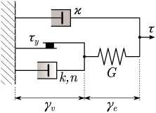
Figure 1: A mechanical analogue of the Saramito-Herschel-Bulkley (SHB) model [31].

Other qualitative differences with the HB model exist. For example, the SHB model allows non-zero rate of strain in the unyielded regions, arising from elastic deformations of the solid phase. Conversely, it is theoretically possible that the rate of strain is zero in yielded material because the stresses there have not had enough time to relax. In particular, in the SHB model, contrary to the HB model, the stresses do not respond instantaneously to changes in the rate of strain; rather, the EVP stress tensor is also a function of all past states of $\dot{\underline{\underline{\gamma}}}$, as in viscoelastic fluids.

Furthermore, as noted in [39, 32], the combination of plastic and elastic terms in the SHB Eq. (7) can produce complex behaviour not observed in either purely viscoplastic or purely viscoelastic flows. One such feature is that the extra stress tensor and the velocity gradient can vary discontinuously across yield surfaces [39]. Another feature is that flows are inherently transient, in the sense that there exist an infinitude of steady states which depend in a continuous manner on the initial conditions. Even if it is just the steady state that is sought, one cannot simply discard the time derivatives in Eqs. (6) and (7); the steady state must be obtained by a transient simulation with appropriate initial conditions. It is not only the steady state stresses that depend on the initial conditions, but also the steady state velocity. This issue was studied in [32] in the context of cylindrical Couette flow. In fact, actual EVP materials do behave this way in experiments, with the steady state depending on the residual stresses present in the unyielded, stationary material at the start of the experiment [32]. The residual stresses are stresses that are “trapped” inside unyielded material because there is no relaxation mechanism there. E.g. for stationary ($\underline{u}=0$) unyielded material, Eq. (7) predicts $\partial\underline{\underline{\tau}}/\partial t=0$. In experiments, residual stresses do develop during the preparation of the material and are difficult to eliminate.

This contrasts the behaviour of classic VP models such as the HB, where there is a stress indeterminacy in the unyielded regions: there exist infinite $\underline{\underline{\sigma}}$ fields within these regions that have the same divergence $\nabla\cdot\underline{\underline{\sigma}}$ which yields $\dot{\underline{\underline{\gamma}}}=0$ when substituted in the momentum equation (6). Each of these fields is a valid solution. The HB steady-state does not depend on the initial conditions, and can be obtained directly, by dropping the time derivative from Eq. (6). The HB model makes no connection between this indeterminacy and the initial conditions, and in fact it even allows that stresses in the unyielded regions vary discontinuously in time. No such indeterminacy is exhibited by the SHB model, the stresses in both the yielded and unyielded regions being precisely determined for given initial conditions.

In the limit of very high elastic modulus, $G\rightarrow\infty$, the SHB material becomes so stiff that it behaves as an inelastic fluid or solid; the importance of the first term on the left-hand side of the SHB constitutive equation (7) diminishes and that equation tends to become identical to the classic HB equation (4). However, it must be kept in mind that the difference in character between the SHB and HB models is in some respects retained no matter how large the value of $G$ is. This concerns mostly the stress state in the unyielded regions, which for the SHB model remains uniquely determined by the initial conditions whereas that of the HB model is indeterminate. Also, as discussed in Appendix A, in the HB model $\underline{\underline{\tau}}$ was defined to equal $\underline{\underline{\sigma}}{}_{d}$ whereas for the SHB model the identification of $\underline{\underline{\tau}}$ with $\underline{\underline{\sigma}}{}_{d}$ as $G\rightarrow\infty$ is not guaranteed.

Figure 1 shows that the complete SHB model contains an additional viscous component labelled $\kappa$ not discussed thus far. This is a Newtonian component, of viscosity $\kappa$, which makes the unyielded phase behave as a Kelvin-Voigt solid. The entire extra stress tensor is then

$$\underline{\underline{\tau_{e}}}\;=\;\underline{\underline{\tau}}\;+\;\kappa\dot{\underline{\underline{\gamma}}}$$ (10)

The SHB model then reduces to the Oldroyd-B viscoelastic model when $\tau_{y}=0$ and $n=1$. However, in the main results of Sec. 6 we will use $\kappa=0$.

Finally, concerning the boundary conditions, we consider solid wall boundaries. We will mostly employ the no-slip condition, but since (elasto)viscoplastic materials are usually slippery we will also employ a Navier slip condition, according to which the relative velocity between the fluid and the wall, in the tangential direction, is proportional to the tangential stress. For two-dimensional flows this is expressed as follows: Let $\underline{n}$ be the unit vector normal to the wall, and $\underline{s}$ be the unit vector tangential to the wall within the plane in which the equations are solved. Let also $\underline{u}$ and $\underline{u}_{w}$ be the fluid and wall velocities, respectively. Then,

$$\left(\underline{u}-\underline{u}_{w}\right)\cdot\underline{s}\;=\;\beta\left(\underline{n}\cdot\underline{\underline{\tau}}\right)\cdot\underline{s}$$ (11)

where the parameter $\beta$ is called the slip coefficient.

2.1 Nondimensionalisation of the governing equations

In the present work we will solve the dimensional governing equations. Nevertheless, nondimensionalisation of the equations reveals a number of dimensionless parameters that characterise the flow. So, let $L$ and $U$ be characteristic length and velocity scales of the problem, with $T=L/U$ the associated time scale, and choose the following characteristic value of stress, $S$ (the Newtonian viscosity $\kappa$, Eq. (10), is omitted):

$$S\;\equiv\;\tau_{y}\;+\;k\left(\frac{U}{L}\right)^{n}$$ (12)

Then, we define the dimensionless variables, denoted with a tilde (~), as $x_{i}=\tilde{x}_{i}L$, $t=\tilde{t}T$, $\underline{u}=\tilde{\underline{u}}U$, $p=\tilde{p}S$, and $\underline{\underline{\tau}}=\tilde{\underline{\underline{\tau}}}S$. Substituting these into the governing equations (5), (6), and (7)-(8), we obtain their dimensionless forms:

$$\tilde{\nabla}\cdot\tilde{u}\;=\;0$$ (13)

$$\operatorname{\mathit{Re}}\left(\frac{\partial\tilde{\underline{u}}}{\partial\tilde{t}}\;+\;\tilde{\nabla}\cdot(\tilde{u}\tilde{u})\right)\;=\;-\tilde{\nabla}\tilde{p}\;+\;\tilde{\nabla}\cdot\tilde{\underline{\underline{\tau}}}$$ (14)

$$\operatorname{\mathit{Wi}}\left(\frac{\partial\tilde{\underline{\underline{\tau}}}}{\partial\tilde{t}}\;+\;\tilde{\underline{u}}\cdot\tilde{\nabla}\tilde{\underline{\underline{\tau}}}\;-\;(\tilde{\nabla}\tilde{\underline{u}})^{\mathrm{T}}\cdot\tilde{\underline{\underline{\tau}}}\;-\;\tilde{\underline{\underline{\tau}}}\cdot\tilde{\nabla}\tilde{\underline{u}}\right)\;+\;\left(\frac{\max\left(0,\tilde{\tau}_{d}-\operatorname{\mathit{Bn}}\right)}{1-\operatorname{\mathit{Bn}}}\right)^{\frac{1}{n}}\frac{1}{\tilde{\tau}_{d}}\;\tilde{\underline{\underline{\tau}}}\;=\;\tilde{\dot{\underline{\underline{\gamma}}}}$$ (15)

where $\tilde{\nabla}=(1/L)\nabla$ and $\tilde{\dot{\underline{\underline{\gamma}}}}=\dot{\underline{\underline{\gamma}}}/(U/L)$. The following dimensionless numbers appear:

Reynolds number $$\operatorname{\mathit{Re}}\;\equiv\;\frac{\rho U^{2}}{S}$$ (16)

Weissenberg number $$\operatorname{\mathit{Wi}}\;\equiv\;\frac{S}{G}$$ (17)

Bingham number $$\operatorname{\mathit{Bn}}\;\equiv\;\frac{\tau_{y}}{S}$$ (18)

A more standard choice for $S$ would account only for viscous effects, omitting plasticity: $S=k(U/L)^{n}$. This would lead to more standard definitions of the Reynolds and Bingham numbers:

$$\operatorname{\mathit{Re}}^{\prime}\; \equiv\;\frac{\rho U^{2-n}L^{n}}{k}\; =\;\frac{\operatorname{\mathit{Re}}}{1-\operatorname{\mathit{Bn}}}$$ (19)

$$\operatorname{\mathit{Bn}}^{\prime}\; \equiv\;\frac{\tau_{y}L^{n}}{kU^{n}}\; =\;\frac{\operatorname{\mathit{Bn}}}{1-\operatorname{\mathit{Bn}}}$$ (20)

However, it was shown in [40] (see also the discussion in [41]) that in viscoplastic flows $\operatorname{\mathit{Re}}$ suffices as a standalone indicator of inertial effects in the flow, whereas $\operatorname{\mathit{Re}}^{\prime}$ does not (the inertial character must be inferred from the values of $\operatorname{\mathit{Re}}^{\prime}$ and $\operatorname{\mathit{Bn}}^{\prime}$ combined). Hence the definition (12) was preferred. Concerning the Bingham number, $\operatorname{\mathit{Bn}}\in[0,1]$ and $\operatorname{\mathit{Bn}}^{\prime}\in[0,\infty)$ are simply related through Eq. (20) and carry exactly the same information. Because of familiarity with $\operatorname{\mathit{Bn}}^{\prime}$ that is almost universally used in the literature, we will use both $\operatorname{\mathit{Bn}}$ and $\operatorname{\mathit{Bn}}^{\prime}$ in this study.

The Weissenberg number $\operatorname{\mathit{Wi}}$ is an indicator of elastic effects in the flow. Unlike the $\operatorname{\mathit{Re}}$ and $\operatorname{\mathit{Bn}}$ numbers, it is not a ratio between stresses of different nature or momentum fluxes. In fact, as seen in the mechanical analogue of Fig. 1, omitting the Newtonian component $\kappa$, the viscoplastic and elastic components are connected in series and thus carry the same load. Therefore, the representative stress $S$, although defined by considerations pertaining to the viscoplastic component of the material behaviour (Eq. (12)), is borne also by the elastic component of the material structure and thus $\operatorname{\mathit{Wi}}\equiv S/G$ is a typical elastic deformation. In the literature, the standard form for the Weissenberg number is $\operatorname{\mathit{Wi}}=\lambda U/L$, where $\lambda$ is a relaxation time, which becomes equivalent to our definition if we define

$$\lambda\;\equiv\;\frac{\eta}{G}\qquad\text{where}\qquad\eta\equiv\frac{S}{U/L}$$ (21)

The relaxation time $\lambda$ is proportional to the apparent viscosity $\eta$ (the more viscous the flow is, the slower the recovery from elastic deformations) and inversely proportional to the elastic modulus $G$ (the stiffer the material is, the faster it recovers). Note that $\lambda$ and $\eta$ as defined by (21) are not material constants but reflect also the influence of the flow, as they depend on $U$ and $L$ in addition to the material parameters $\tau_{y}$, $G$, $k$ and $n$ (Eq. (12)). The definition $\operatorname{\mathit{Wi}}=\lambda U/L$ is also interpreted as a typical elastic strain: it is the product of the strain rate $U/L$ by the time period $\lambda$ during which the material has not yet significantly relaxed.

Finally, an important dimensionless number is the yield strain,

$$\gamma_{y}\;=\;\frac{\tau_{y}}{G}\;=\;\operatorname{\mathit{Bn}}\cdot\operatorname{\mathit{Wi}}$$ (22)

which depends only on the material parameters and not on kinematic or geometric parameters of the flow such as $U$ and $L$. The fact that it is equal to the product of $\operatorname{\mathit{Bn}}$ and $\operatorname{\mathit{Wi}}$ means that these two numbers are not independent but their product is constant for a given material. Since $\operatorname{\mathit{Bn}}\in[0,1]$, it follows that $\operatorname{\mathit{Wi}}\in[\gamma_{y},\infty)$. That $\operatorname{\mathit{Wi}}$ is bounded from below by $\gamma_{y}$ follows also directly from the definitions (17) and (12), and derives from the characteristic stress definition (12) which assumes the existence of unyielded regions; in such regions the strain, of which $\operatorname{\mathit{Wi}}$ is a measure, is higher than the yield strain $\gamma_{y}$.

3 Discretisation of the governing equations

3.1 Preliminary considerations

In this section we propose a Finite Volume Method (FVM) for the discretisation of the governing equations. The method will be described for two-dimensional problems, but extension to three dimensions is straightforward. The first step is the tessellation of the domain $\Omega$ into a number of non-overlapping volumes, or cells. Each cell is bounded by straight faces, each of which separates it from another single cell or from the exterior of the domain (the latter are called boundary faces). Figure 2 shows such a cell $P$ along with its faces and neighbours, and the associated nomenclature. Our FVM is applicable to grids of arbitrary polygonal cells, although for the results of Sec. 6 we will employ Cartesian grids due to the regularity of the problem geometry. Grids will be labelled after a characteristic cell length $h$.

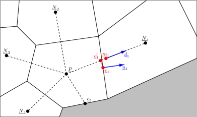
Figure 2: Cell $P$ and its neighbouring cells, each having a single common face with $P$. Its faces and neighbours are numbered in anticlockwise order, with face $f$ separating $P$ from its neighbour $N_{f}$. The shaded area lies outside the domain, so face 5 is a boundary face. The geometric characteristics of face 1 are displayed. The position vectors of the centroids of cells $P$ and $N_{f}$ are denoted as $\underline{P}$ and $\underline{N}_{f}$; $\underline{c}_{f}$ is the centroid of face $f$ and $\underline{c}^{\prime}_{f}$ is its closest point on the line connecting $\underline{P}$ and $\underline{N}_{f}$; $\underline{m}_{f}$ is the midpoint between $\underline{P}$ and $\underline{N}_{f}$; $\underline{n}_{f}$ is the unit vector normal to face $f$, pointing outwards of $P$, and $\underline{d}_{f}$ is the unit vector pointing from $\underline{P}$ towards $\underline{N}_{f}$. The volume of cell $P$ is denoted as $\Omega_{P}$.

The discretisation procedure will convert the governing equations into a large set of algebraic equations involving only (approximate) values of the dependent variables at the cell centroids. These values will be denoted using the cell index as a subscript, i.e. $\phi_{P}$ is the value of the variable $\phi$ at the centroid of cell $P$; if the variable name already includes a subscript then the cell index will be separated by a comma (e.g. $\tau_{d,P}$ is the deviatoric stress at cell $P$). We aim for a second-order accurate method, i.e. one whose discretisation error scales as $h^{2}$. With the present governing equations, a difficulty arises from the fact that they all contain only first spatial derivatives because this allows the development of spurious oscillations in the solution. For example, assume that on the grid of Fig. 3, a quantity $\phi$ has the value zero at the boundary points ($\bullet$), the value $+1$ at points ($\blacktriangle$), and the value $-1$ at points ($\blacktriangledown$). FVM integration of first derivatives of $\phi$ over each cell eventually comes down to a calculation involving values of $\phi$ at face centres ($\circ$) and ($\bullet$), due to application of the Gauss theorem. If we use linear interpolation to approximate the values of $\phi$ at the face centroids ($\circ$) from the values at the cell centres on either side of each face, then we obtain $\phi=0$ at every face centre ($\circ$). This ultimately results in obtaining a zero integral of the first derivative of $\phi$ over any cell. Thus, interpolation filters out the oscillating cell-centre field and leaves a smooth field over the face centres, which in turn produces an image of the discrete operator that varies smoothly from one cell to the next.

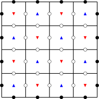
Figure 3: A checkerboard distribution of values on a Cartesian grid. Different values are stored at points $\blacktriangle$ and $\blacktriangledown$.

To see how this creates a problem, consider the FVM discretisation on grid $h$ of the following PDE

$$f(\phi)\;=\;b$$ (23)

where $b$ is a known function. The FVM produces a system of algebraic equations that can be written as

$$F_{h}(\phi_{h})\;=\;B_{h}$$ (24)

where $\phi_{h}$ is the vector of unknown values of $\phi$ at the cell centroids, $F_{h}$ is the discrete operator representing the integral of the differential operator $f$ over each cell, and $B_{h}$ is the vector of integrals of the known function $b$ over each cell. The aforementioned filtering action of the face interpolation scheme means that $F_{h}$ will filter out any oscillations in $\phi_{h}$, producing a smooth image $F_{h}(\phi_{h})$; therefore, the solution $\phi_{h}$ to the system (24) can be oscillatory even if the right-hand side $B_{h}$ is smooth. This is not just a remote possibility, but it does occur in practice, a notorious example being the spurious pressure oscillations produced by the FVM solution of the Navier-Stokes equations (see [42] for a demonstration). But, if the discretisation schemes incorporated in the operator $F_{h}$ are designed so as to reflect any oscillations in the vector $\phi_{h}$ onto the image $F_{h}(\phi_{h})$, then for a smooth right-hand side $B_{h}$ the system (24) can only have a smooth solution $\phi_{h}$. For the Navier-Stokes equations, the main concern is the pressure oscillations because any velocity oscillations will be reflected onto the second derivatives of velocity present in the momentum equations and are therefore inhibited. But in our case, all three of the governing equations, (5), (6) and (7)–(8), only contain first derivatives and thus we have to be concerned about the possibility of spurious oscillations in all three variables $\underline{u}$, $p$, and $\underline{\underline{\tau}}$. In the following subsections the adopted measures will be described.

In what follows we will need a “characteristic viscosity”, a quantity with units of viscosity somewhat characteristic of the flow’s viscous character. Our first choice is the following:

$$\eta_{a}\;\equiv\;\kappa\;+\;\frac{S}{U/L}$$ (25)

where $S$ is given by (12). This value is constant throughout the domain. A second option we tried is similar to the coefficient of the DAVSS-G technique proposed in [43] and varies throughout the domain, depending on the ratio between the magnitudes of the stress and rate-of-strain tensors:

$$\eta_{a}\;\equiv\;\kappa\;+\;\frac{1}{2}\,\frac{S}{U/L}\;+\;\frac{1}{2}\,\frac{S\,+\,\tau_{P}\,+\,\tau_{N_{f}}}{U/L\,+\,\dot{\gamma}_{P}\,+\,\dot{\gamma}_{N_{f}}}$$ (26)

The above formula gives $\eta_{a}$ at face $f$ of cell $P$. With definition (26), $\eta_{a}$ never falls below $\kappa+0.5S/(U/L)$, tends to $\kappa+S/(U/L)$ when both $\tau$ and $\dot{\gamma}$ are small, and tends to $\kappa+0.5S/(U/L)+\tau/\dot{\gamma}$ when both $\tau$ and $\dot{\gamma}$ are large. Also, it does not tend to infinity when $\dot{\gamma}\rightarrow 0$, although it has no upper bound.

The discretisation of several terms (e.g. the calculation of $\underline{\underline{\dot{\gamma}}}\equiv\nabla\underline{u}+(\nabla\underline{u})^{\mathrm{T}}$ and its magnitude) requires the use of a discrete gradient operator which approximates $\nabla\phi$ at the cell centres. We employ the least-squares operator described in detail in [44], denoted here as $\nabla_{h}^{q}$, the superscript $q$ being the exponent employed; in [44] it was shown that on smooth structured grids the choice $q=1.5$ engenders second-order accuracy ($\nabla_{h}^{1.5}\phi=\nabla\phi+O(h^{2})$) while with other $q$ values the accuracy degrades to first-order at boundary cells. On irregular (unstructured) grids all choices of $q$ result in first order accuracy everywhere. Nevertheless, first-order accurate gradients suffice for second-order accuracy of the differentiated variables, i.e. are compatible with second-order accurate FVMs [44].

Finally, linear interpolation for calculating face centre values on unstructured grids is performed as

$$\bar{\phi}_{c_{f}}\;=\;\bar{\phi}_{c^{\prime}_{f}}\;+\;\bar{\nabla}^{q}_{h}\phi_{c^{\prime}_{f}}\!\cdot\!(\underline{c}_{f}-\underline{c}^{\prime}_{f})$$ (27)

where the overbar denotes an interpolated value, and in the right-hand side both $\phi$ and its gradient are interpolated linearly to point $\underline{c}^{\prime}_{f}$ (the closest point to the face centre lying on the line joining $\underline{P}$ to $\underline{N}_{f}$, Fig. 2) according to the formula

$$\bar{\phi}_{c^{\prime}_{f}}\;\equiv\;\frac{\|\underline{c}^{\prime}_{f}-\underline{N}_{f}\|}{\|\underline{N}_{f}-\underline{P}\|}\,\phi_{P}\;+\;\frac{\|\underline{c}^{\prime}_{f}-\underline{P}\|}{\|\underline{N}_{f}-\underline{P}\|}\,\phi_{N_{f}}$$ (28)

3.2 Discretisation of the continuity equation

Integrating Eq. (5) over cell $P$ and applying the divergence theorem, we get the mass flux balance for that cell:

$$\sum_{f}\int_{s_{f}}\underline{n}\cdot\left(\rho\underline{u}\right)\,\mathrm{d}s\;=\;0$$ (29)

where $s_{f}$ is the surface of face $f$, $\underline{n}$ is the outward (of $P$) unit vector normal to that face, and $\mathrm{d}s$ is an infinitesimal surface element. The integrals summed are the outward mass fluxes through the respective faces of cell $P$. They are approximated by midpoint rule integration with additional stabilising terms:

$$\int_{s_{f}}\underline{n}\cdot\left(\rho\underline{u}\right)\,\mathrm{d}s\;\approx\;\rho\,s_{f}\,\left[\bar{\underline{u}}{}_{c_{f}}\!\cdot\underline{n}{}_{f}\;+\;u^{p+}_{f}\;-\;u^{p-}_{f}\right]\;\equiv\;\dot{M}_{f}$$ (30)

where

$$u^{p+}_{f}\; \equiv\;a_{f}^{mi}\left(p_{P}-p_{N_{f}}\right)$$ (31)

$$u^{p-}_{f}\; \equiv\;a_{f}^{mi}\>\bar{\nabla}^{q}_{h}p_{m_{f}}\cdot(\underline{P}-\underline{N}{}_{f}),\qquad\bar{\nabla}^{q}_{h}p_{m_{f}}\;\equiv\;\frac{1}{2}\left(\nabla^{q}_{h}p_{P}+\nabla^{q}_{h}p_{N_{f}}\right)$$ (32)

$$a_{f}^{mi}\; \equiv\;\frac{1}{\rho\left(\|\underline{u}_{N_{f}}-\underline{u}_{P}\|\>+\>\dfrac{h_{f}}{\Delta t}\right)\;+\;\dfrac{2\eta_{a}}{h_{f}}},\qquad h_{f}\;\equiv\;\left[\frac{1}{2}\left(\Omega_{P}+\Omega_{N_{f}}\right)\right]^{\frac{1}{D}}$$ (33)

where $\Delta t$ is the current time step (see Sec. 3.5), $\Omega_{P}$ and $\Omega_{N_{f}}$ are the cell volumes, and $D$ equals either 2 or 3, for 2D and 3D problems, respectively. With the definition (30), the discrete version of the continuity equation for a cell $P$ is

$$\sum_{f}\dot{M}_{f}\;=\;0$$ (34)

To expound the above scheme, we make the following remarks:

Remark 1: If $u_{f}^{p+}$ and $u_{f}^{p-}$ are omitted from Eq. (30) then we are left with simple midpoint rule integration ($\bar{\underline{u}}{}_{c_{f}}$ is obtained using the scheme (27)). The part of $\dot{M}_{f}$ due to $u_{f}^{p+}$ and $u_{f}^{p-}$ can be viewed as belonging to the truncation error of the continuity equation of cell $P$:

$$\frac{1}{\Omega_{P}}\rho\,s_{f}\left(u_{f}^{p+}-u_{f}^{p-}\right)\;=\;\frac{\rho\,s_{f}}{\Omega_{P}}a_{f}^{mi}\left[\left(p_{P}-p_{N_{f}}\right)\>-\>\bar{\nabla}^{q}_{h}p_{m_{f}}\cdot(\underline{P}-\underline{N}{}_{f})\right]$$ (35)

(the truncation error is defined per unit volume, hence we divide by the cell volume $\Omega_{P}$). It is easy to show, by expanding the pressure in a Taylor series about point $\underline{m}_{f}$ (Fig. 2), that $(p_{P}-p_{N_{f}})-\nabla p(\underline{m}_{f})\cdot(\underline{P}-\underline{N}_{f})=O(h^{3})$. However, since we use only an approximation to the pressure gradient, $\nabla_{h}^{q}p=\nabla p+O(h)$, the term in square brackets in Eq. (35) is $O(h^{2})$ (because $O(h)\cdot(\underline{P}-\underline{N}_{f})=O(h^{2})$). Given also that $\Omega_{P}=O(h^{2})$, $s_{f}=O(h)$ and $a_{f}^{mi}=O(h)$, the whole term (35) is $O(h^{2})$, which is compatible with a second-order accurate method such as the present one.

Remark 2: The term (35) inhibits spurious pressure oscillations by reflecting them on the image of the discrete continuity operator (see Eq. (24) and associated discussion). Pressure oscillations cause the term $u_{f}^{p+}$ to oscillate from face to face, and are thus reflected on the continuity image. On the other hand, such oscillations are filtered out by the gradient operator $\nabla_{h}^{q}$, so that the term $u_{f}^{p-}$ varies smoothly from face to face (it does not pass the oscillations on to the image). The $u_{f}^{p-}$ term is used simply for counterbalancing the truncation error introduced by $u_{f}^{p+}$.

Remark 3: The coefficient $a_{f}^{mi}$ is chosen so that the terms $u_{f}^{p+}$ and $u_{f}^{p-}$ of the mass flux expression (30), which have units of velocity, are neither too small to have a stabilising effect nor so large that they dominate the mass flux. The “velocities” $u_{f}^{p+}$ and $u_{f}^{p-}$ are functions of local pressure variations, and attempt to quantify the contributions of these pressure variations to the velocity field. Pressure and velocity are connected through the momentum equation, so consider this equation in the following non-conservative form, where we assume that the stress tensor can be approximated through the use of a characteristic viscosity such as (25) or (26) as $\underline{\underline{\tau}}\approx\eta(\nabla\underline{u}+(\nabla\underline{u})^{\mathrm{T}})$:

$$\rho\left(\frac{\partial\underline{u}}{\partial t}\>+\;\underline{u}\cdot\nabla\underline{u}\right)\;=\;-\nabla p\;+\;\nabla\cdot(\eta\nabla\underline{u})$$ (36)

where we have neglected the term $\nabla\cdot(\eta(\nabla\underline{u})^{\mathrm{T}})$, assuming that it is small (it is zero if $\eta$ is constant). We are free to make these sorts of approximations because all we want is a rough estimate of the effect that the pressure gradient has on velocity. So, consider the simple uniform grid, of spacing $h$, shown in Fig. 4, where $u$ denotes the velocity component normal to the face separating cells $P$ and $N$. We will employ a simple FV discretisation of Eq. (36) in order to relate the velocity $u_{c}$ at the face centre $c$ to the pressures at the centres of the adjacent cells $P$ and $N$. The momentum conservation, Eq. (36), in the direction $x$ normal to the face, for the imaginary cell drawn in dashed line surrounding that face, can be discretised as

$$\rho\frac{u_{c}-u_{c}^{old}}{\Delta t}h^{2}\;+\;\rho u_{c}\left.\frac{\mathrm{d}u}{\mathrm{d}x}\right|_{c}h^{2}\;=\;-\frac{p_{N}-p_{P}}{h}h^{2}\;+\;\frac{1}{h}\left(\eta_{N}\frac{u_{c_{N}}-u_{c}}{h}-\eta_{P}\frac{u_{c}-u_{c_{P}}}{h}\right)h^{2}$$ (37)

where $u_{c}^{\mathrm{old}}$ was the velocity at time $\Delta t$ ago. Assuming that $(\eta_{N}+\eta_{P})u_{c}\approx 2\eta_{c}u_{c}$ we can solve this for $u_{c}$:

$$u_{c}\;=\;\frac{1}{\rho\left(\left.\dfrac{\mathrm{d}u}{\mathrm{d}x}\right|_{c}h\>+\;\dfrac{h}{\Delta t}\right)\;+\;\dfrac{2\eta_{c}}{h}}\,\left(p_{P}-p_{N}\right)\;+\;\cdots$$ (38)

where the dots ($\cdots$) denote the terms that are not related to pressure. The above equation provides a quantification of the local effect of pressure gradient on velocity. It was derived from a simplistic one-dimensional consideration; for more general flows, the coefficient $a_{f}^{mi}$ (33) can be seen to be a generalisation of the coefficient multiplying the pressure difference in Eq. (38). It should be noted that the one-dimensional momentum equation (37) accounts for the viscous force due to the velocity variation in the direction perpendicular to the face, but omits that due to the velocity variation in the direction parallel to the face; had the latter also been accounted for, the viscous term in the denominator of (38), and of $a_{f}^{mi}$ (33), would have been $4\eta/h$ (or $6\eta/h$ in 3D) instead of $2\eta/h$, which would have reduced the magnitude of the stabilisation terms in the mass flux scheme (30), but would also likely somewhat increase the accuracy, according to the results of Sec. 5. We did not investigate this issue further, but the choice is not crucial as it affects neither the stabilisation ability of the technique nor the $O(h^{2})$ magnitude of the error (35) that it introduces.

Figure 4: A row of grid cells.

Remark 4: An explanation of how the scheme retains its oscillation-inhibiting effect when $h\rightarrow 0$ despite $u_{f}^{p+}$, $u_{f}^{p-}$ tending to zero is given in Appendix B.

The scheme (30) – (33) is a variant of the popular technique known as momentum interpolation, which was originally proposed in [45]. Ever since, many variants of this technique have been proposed (see [46] and references therein) almost all of which are intertwined with the SIMPLE algebraic solver (exceptions include [47, 42]). Although this connection with SIMPLE can be useful in some respects [48], and SIMPLE is employed in the present work, we prefer an independent method such as the presently proposed because it is more general, transparent, and easily adaptable. It can be used with other algebraic solvers such as Newton’s method, and it does not lead to dependence of the solution on underrelaxation factors.

3.3 Discretisation of the momentum equation

As for the continuity equation, the FVM discretisation of the momentum equation (6) begins by integrating it over a cell $P$ and applying the divergence theorem, to get

$$\int_{\Omega_{P}}\frac{\partial(\rho\underline{u})}{\partial t}\,\mathrm{d}\Omega\;+\;\sum_{f}\int_{s_{f}}\underline{n}\cdot\left(\rho\underline{u}\underline{u}\right)\,\mathrm{d}s\;=\;-\sum_{f}\int_{s_{f}}\underline{n}\,p\,\mathrm{d}s\;+\;\sum_{f}\int_{s_{f}}\underline{n}\cdot\underline{\underline{\tau}}\,\mathrm{d}s$$ (39)

Using midpoint rule integration, the above equation is approximated by

$$\left.\frac{\partial(\rho\underline{u})}{\partial t}\right|^{a}_{P}\Omega_{P}\;+\;\sum_{f}\dot{M}_{f}\,\bar{\underline{u}}{}_{c_{f}}\;=\;-\sum_{f}\bar{p}_{c_{f}}\,s_{f}\,\underline{n}{}_{f}\;+\;\sum_{f}\underline{F}^{\tau}_{f}$$ (40)

where $\partial/\partial t|^{a}_{P}$, the approximate time derivative at $\underline{P}$, will be defined in Sec. 3.5, $\dot{M}_{f}$ is the mass outflux through face $f$ defined by Eq. (30), $\bar{\underline{u}}{}_{c_{f}}$ and $\bar{p}_{c_{f}}$ are approximated from cell-centre values with the interpolation scheme (27), and $\underline{F}^{\tau}_{f}$ is the approximation of the force on face $f$ due to the EVP stress tensor $\underline{\underline{\tau}}$. Note that Eq. (40) is a vector equation, with two (in 2D) or three (in 3D) scalar components. The force $\underline{F}^{\tau}_{f}$ is calculated as

$$\int_{s_{f}}\underline{n}\cdot\underline{\underline{\tau}}\,\mathrm{d}s\;\approx\;\underline{F}^{\tau}_{f}\;\equiv\;s_{f}\,\left[\underline{n}{}_{f}\cdot\bar{\underline{\underline{\tau}}}{}_{c_{f}}\;+\;\underline{D}^{\tau+}_{f}\;-\;\underline{D}^{\tau-}_{f}\right]$$ (41)

Again, the stress tensor at the face centroid, $\bar{\underline{\underline{\tau}}}{}_{c_{f}}$, is calculated via the linear interpolation scheme (27) (applied component-wise). The viscous pseudo-stresses $\underline{D}_{f}^{\tau+}$ and $\underline{D}_{f}^{\tau-}$ are stabilisation terms employed to suppress spurious velocity oscillations. They are vectors, whose $i$-th components are

$$D_{f,i}^{\tau+}\; \equiv\;\eta_{a}\frac{u_{i,N_{f}}-u_{i,P}}{\|\underline{N}_{f}-\underline{P}\|}$$ (42)

$$D_{f,i}^{\tau-}\; \equiv\;\eta_{a}\bar{\nabla}^{q}_{h}u_{i,m_{f}}\cdot\underline{d}_{f},\qquad\bar{\nabla}^{q}_{h}u_{i,m_{f}}\;\equiv\;\frac{1}{2}\left(\nabla^{q}_{h}u_{i,P}+\nabla^{q}_{h}u_{i,N_{f}}\right)$$ (43)

where $u_{i}$ is the $i$-th velocity component ($\underline{u}=(u_{1},u_{2})$ in 2D), and $\underline{d}_{f}=(\underline{N}_{f}-\underline{P})/\|\underline{N}_{f}-\underline{P}\|$ is the unit vector pointing from $\underline{P}$ to $\underline{N}_{f}$ (Fig. 2). It can be seen that both $D_{f,i}^{\tau+}$ and $D_{f,i}^{\tau-}$ equal a characteristic viscosity, given by (25) or (26), times the velocity gradient in the direction $\underline{d}_{f}$, albeit calculated differently: the gradient as computed in $D_{f,i}^{\tau+}$ is sensitive to velocity oscillations whereas that computed in $D_{f,i}^{\tau-}$ is not. The mechanism of oscillation suppression is similar to that for momentum interpolation: in the presence of spurious velocity oscillations, the smooth part of $D_{f,i}^{\tau+}$ is cancelled out by $D_{f,i}^{\tau-}$, but the oscillatory part produces oscillations in the operator image (in $F_{h}(\phi_{h})$, in the terminology of Eq. (24)).

In the context of colocated FVMs for viscoelastic flows, this technique was first proposed in [26], inspired from the corresponding “momentum interpolation” technique for pressure. A question concerning the method is the appropriate choice of the parameter $\eta_{a}$. The original method [26] as well as some subsequent variants (e.g. [49, 50]), similarly to the original momentum interpolation [45], derived the coefficient from the SIMPLE matrix of the linearised discrete constitutive equation, arriving at complicated expressions. The present simpler approach is essentially equivalent to that adopted by [51, 52] who, for viscoelastic flows, set the coefficient $\eta_{a}$ equal to the polymeric viscosity. The aim is that $\underline{D}_{f}^{\tau+}$ and $\underline{D}_{f}^{\tau-}$ are of the same order of magnitude as the EVP stress acting on the cell face, and this can be achieved using a characteristic viscosity $\eta_{a}$ defined as the ratio of a typical stress to a typical rate of strain for the given problem.

The present technique can also be interpreted as a “both-sides diffusion” technique [52] where the momentum equation discretised by the FVM is not (6) but an equivalent equation where the same diffusion term $\nabla\cdot(\eta_{a}\nabla\underline{u})$ has been subtracted from both sides:

$$\frac{\partial(\rho\underline{u})}{\partial t}\;+\;\nabla\cdot\left(\rho\underline{u}\underline{u}\right)\;-\;\nabla\cdot(\eta_{a}\nabla\underline{u})\;=\;-\nabla p\;+\;\nabla\cdot\underline{\underline{\tau}}\;-\;\nabla\cdot(\eta_{a}\nabla\underline{u})$$ (44)

The left-hand side such term is not discretised in the same way as the right-hand side term; in particular, the component $\underline{D}_{f}^{\tau+}$ in (41) comes from the discretisation of the left-hand side term, whereas the component $\underline{D}_{f}^{\tau-}$ comes from the discretisation of the right-hand side term. The other components of these diffusion terms are discretised in exactly the same way for both of them and cancel out, leaving only $\underline{D}_{f}^{\tau+}$ and $\underline{D}_{f}^{\tau-}$. Since both of these diffusion terms are discretised by central differences they contribute $O(1)$ to the truncation error [44] but $O(h^{2})$ to the discretisation error. In particular, consider that Eq. (44) corresponds to Eq. (23), and its FVM discretisation with the present schemes leads to the algebraic system (24), with the dependent variable $\phi\equiv\underline{u}$ being the velocity. If $\phi^{e}$ is the exact velocity (the solution of Eq. (23)) and $\phi$ is the approximate velocity obtained by solving the system (24), then the discretisation error is $\varepsilon=\phi^{e}-\phi$. The latter is related to the truncation error $\alpha$ by $F^{\prime}_{h}(\phi_{h})\cdot\varepsilon_{h}\approx-\alpha_{h}$, where $F^{\prime}_{h}(\phi_{h})$ is the Jacobian matrix of the operator $F_{h}$ evaluated at the approximate solution $\phi_{h}$ (see e.g. [53] for a derivation). Let us focus on the $\nabla\cdot(\eta_{a}\nabla\underline{u})$ term of the left-hand side of (44), which is discretised with a compact stencil giving rise to the $\underline{D}_{f}^{\tau+}$ term of the scheme (41) (a similar analysis of the term on the right-hand side can be made). Because the diffusion operator is linear, its contribution to the truncation error $F^{\prime}_{h}(\phi_{h})\cdot\varepsilon_{h}$ is equal to its contribution to $F_{h}(\varepsilon_{h})$, i.e. it can be calculated by replacing the velocities by their discretisation errors in (42) (we neglect the rest of the contributions, which cancel out with the corresponding ones of the diffusion term of the right side of Eq. (44)). So, plugging $\varepsilon$ into Eq. (42) instead of $u_{i}$ we get a contribution to the truncation error of cell $P$ of $(s_{f}/\Omega_{P})\eta_{a}(\varepsilon_{N_{f}}-\varepsilon_{P})/\|\underline{N}_{f}-\underline{P}\|=O(h^{-2})(\varepsilon_{N_{f}}-\varepsilon_{P})$. If our method is second-order accurate then $\varepsilon=O(h^{2})$. On unstructured grids, the variation of discretisation error in space has a random component [53] so that $\varepsilon_{N_{f}}-\varepsilon_{P}=O(h^{2})$ as well, which results in a $O(1)$ contribution to the truncation error. On smooth structured grids the discretisation error varies smoothly [53] so that $\varepsilon_{N_{f}}-\varepsilon_{P}=O(h^{3})$ and each face contributes $O(h)$ to the truncation error (on such grids there is also a cancellation between opposite faces for each cell which reduces the net contribution to the truncation error to $O(h^{2})$).

Another benefit that comes from the incorporation of the stabilisation terms in the scheme (41) concerns the algebraic solver, SIMPLE [54]. Within each SIMPLE iteration a succession of linearised systems of equations are solved, one for each dependent variable. The systems for the velocity components $u_{i}$ are derived from linearisation of the (discretised) momentum equation (6). The latter, unlike in (generalised) Newtonian flows, contains no diffusion terms and the velocity appears directly only in the convection terms of the left-hand side. In low Reynolds number flows, these terms play only a minor role and the momentum balance involves mainly the pressure and stress. Constructing the linear systems for the velocity components only from these inertial terms would lead to bad convergence of the SIMPLE algorithm. Nevertheless, velocity plays an important indirect role in the momentum equation through the EVP stress tensor, to which it is related via the constitutive equation (7). Therefore, either the momentum and constitutive equations have to be solved in a coupled manner, or the effect of velocity on the stress tensor has to somehow be directly quantified in the momentum equation, which is precisely what the stabilisation term $\underline{D}_{f}^{\tau+}$ achieves; in particular, the diffusion term on the left-hand side of Eq. (44) contributes to the matrix of coefficients of the linear systems for $u_{i}$, making this matrix very similar to those for (generalised) Newtonian flows.

Finally, the momentum balance for cells that lie at the wall boundaries involves the pressure and the stress tensor at these boundaries. The pressure is linearly extrapolated from the interior, as is a common practice [55]. For stress two possible options are linear extrapolation, as for pressure, and the imposition of a zero-gradient condition which is roughly equivalent to setting the stress at the boundary face equal to that at the owner cell centre. In [56], the former approach was found, as expected, to be more accurate, while the latter was found to be more robust. In the present work we employed either linear extrapolation or a modified extrapolation which is akin to the scheme (41). So, if $b$ is a boundary face of cell $P$, the linearly extrapolated value of stress at its centre is calculated as

$$\bar{\underline{\underline{\tau}}}{}_{c_{b}}\;=\;\underline{\underline{\tau}}{}_{P}\;+\;\nabla_{h}^{1}\underline{\underline{\tau}}{}_{P}\cdot(\underline{c}_{b}-\underline{P})$$ (45)

where the least-squares stress gradient $\nabla_{h}^{1}\underline{\underline{\tau}}{}_{P}$ is calculated with $q=1$ and using only the stress values at the centres of $P$ and its neighbour cells. This scheme is used also for extrapolation of pressure, but when it comes to stress we can go a step further: the force due to the EVP stress tensor on boundary face $b$ can be calculated by a scheme that has precisely the form (41) only that the interpolated stress $\bar{\underline{\underline{\tau}}}{}_{c_{f}}$ (27) is replaced by the extrapolated value $\bar{\underline{\underline{\tau}}}{}_{c_{b}}$ (45) and the $D$ terms are replaced by

$$D_{b,i}^{\tau+}\; \equiv\;\eta_{a}\frac{u_{i,c_{b}}-u_{i,P}}{\|\underline{c}_{b}-\underline{P}\|}$$ (46)

$$D_{b,i}^{\tau-}\; \equiv\;\eta_{a}\bar{\nabla}^{q}_{h}u_{i,m_{b}}\cdot\underline{d}_{b}$$ (47)

where $\underline{d}_{b}$ is the unit vector pointing from $\underline{P}$ to $\underline{c}_{b}$ and the gradient in (47) is extrapolated to point $\underline{m}_{b}\equiv(\underline{P}+\underline{c}_{b})/2$ via the scheme (45) with $\underline{c}_{b}$ replaced by $\underline{m}_{b}$. The terms (46) – (47) do not have an apparent stabilising effect, and in fact our experience has shown that they sometimes can cause convergence difficulties to the algebraic solver. Such is the case with wall slip examined in Sec. 6.4, where we had to set these terms to zero and use simple linear extrapolation of stresses at the walls. Nevertheless, we also found that these terms can increase the accuracy of the solution (see Sec. 5) and therefore we employed them whenever possible (they were used for all the main results except those of Sec. 6.4).

3.4 Discretisation of the constitutive equation

Again, by integrating the SHB equation (7) – (8) and applying the divergence theorem we obtain

$$\int_{\Omega_{P}}\frac{\partial\underline{\underline{\tau}}}{\partial t}\,\mathrm{d}\Omega\;+\;\sum_{f}\int_{s_{f}}\underline{n}\cdot\underline{u}\underline{\underline{\tau}}\,\mathrm{d}s\;=\;$$

$$G\int_{\Omega_{P}}\dot{\underline{\underline{\gamma}}}\,\mathrm{d}\Omega\;-\;G\int_{\Omega_{P}}\left(\frac{\max(0,\tau_{d}-\tau_{y})}{k}\right)^{\frac{1}{n}}\frac{1}{\tau_{d}}\;\underline{\underline{\tau}}\,\mathrm{d}\Omega\;+\;\int_{\Omega_{P}}\left((\nabla\underline{u})^{\mathrm{T}}\cdot\underline{\underline{\tau}}\;+\;\underline{\underline{\tau}}\cdot\nabla\underline{u}\right)\mathrm{d}\Omega$$ (48)

The surface integral on the left-hand side derives from application of the divergence theorem to the second term on the right-hand side of Eq. (8), using the identity $\underline{u}\cdot\nabla\underline{\underline{\tau}}=\nabla\cdot(\underline{u}\underline{\underline{\tau}})-(\nabla\cdot\underline{u})\underline{\underline{\tau}}$ and the incompressibility condition $\nabla\cdot\underline{u}=0$. Equation (48) has the form of a conservation equation for stress. In the left-hand side, there is the rate of change of stress in the volume plus the outflux of stress, which equal the rate of change of stress in a fixed mass of fluid moving with the flow. In the right-hand side, there are three source terms which express, respectively, stress generation (the $\dot{\underline{\underline{\gamma}}}$ term), relaxation (the viscous term), and transformation (the upper convective derivative term). Equation (48) is then discretised as:

$$\left.\frac{\partial\underline{\underline{\tau}}}{\partial t}\right|^{a}_{P}\Omega_{P}\;+\;\frac{1}{\rho}\sum_{f}\dot{M}_{f}\bar{\underline{\underline{\tau}}}{}^{{}_{C}}_{c_{f}}\;=\;$$

$$G\,\Omega_{P}\,\dot{\underline{\underline{\gamma}}}{}_{P}\;-\;G\,\Omega_{P}\,\left(\frac{\max(0,\tau_{d,P}-\tau_{y})}{k}\right)^{\frac{1}{n}}\frac{1}{\tau_{d,P}}\;\underline{\underline{\tau}}{}_{P}\;+\;\Omega_{P}\,\left((\nabla_{h}^{q}\underline{u})^{\mathrm{T}}_{P}\cdot\bar{\underline{\underline{\tau}}}{}_{P}\;+\;\bar{\underline{\underline{\tau}}}{}_{P}\cdot\nabla_{h}^{q}\underline{u}_{P}\right)$$ (49)

where $\partial/\partial t|^{a}_{P}$ is the approximate time derivative at $\underline{P}$ (Sec. 3.5), $\dot{M}_{f}$ is the mass flux (30), $\dot{\underline{\underline{\gamma}}}{}_{P}=\nabla_{h}^{q}\underline{u}_{P}+(\nabla_{h}^{q}\underline{u})^{\mathrm{T}}_{P}$ is the discrete value of $\dot{\underline{\underline{\gamma}}}$ at $\underline{P}$, and $\tau_{d,P}$ is the value of $\tau_{d}$ at $\underline{P}$, calculated from $\underline{\underline{\tau}}{}_{P}$ via Eq. (9).

In the convection term of Eq. (49) (the second term on the left-hand side), $\bar{\underline{\underline{\tau}}}{}^{{}_{C}}_{c_{f}}$ is the value of $\underline{\underline{\tau}}$ interpolated at the face centre $\underline{c}_{f}$, but not by the linear interpolation (27). Since the constitutive equation lacks diffusion terms, there is a danger of spurious stress oscillations, and a common preventive measure is to use so-called high resolution schemes [57] for the discretisation of the convection term. In viscoelastic flows, the CUBISTA scheme [58] has proved to be effective and is widely adopted (e.g. [59, 60, 61, 29]). In the present work, we adapted it for use on unstructured grids as follows. To account for skewness, a scheme similar to (27) is used, but the value at point $\underline{c}^{\prime}_{f}$ is interpolated with CUBISTA:

$$\bar{\phi}^{{}_{C}}_{c_{f}}\;=\;\bar{\phi}^{{}_{C}}_{c^{\prime}_{f}}\;+\;\bar{\nabla}^{q}_{h}\phi_{c^{\prime}_{f}}\!\cdot\!(\underline{c}_{f}-\underline{c}^{\prime}_{f})$$ (50)

Note that the second term of the right-hand side is exactly the same as for the scheme (27) (the gradient is interpolated linearly). The first term of the right-hand side is the value at point $\underline{c}^{\prime}_{f}$ interpolated via CUBISTA. CUBISTA is a high-resolution scheme based on the Normalised Variable Formulation [62], and on structured grids such schemes interpolate the value at a face from the values at two upwind cell centres and one downwind cell centre; these are the two cells on either side of the face, labelled $P$ and $D$ in Fig. 5, and a farther cell $U$. But on an unstructured grid the farther-upwind cell $U$ is not straightforward (or even not possible) to identify. To overcome this hurdle, we follow an approach [63, 57] which is based on the observation that, on a uniform structured grid such as that shown in Fig. 5, it holds that

$$\phi_{U}\;=\;\phi_{D}\;-\;\nabla_{h}^{q}\phi_{P}\cdot(\underline{D}-\underline{U})$$ (51)

because the least-squares gradient is such that $\nabla_{h}^{q}\phi_{P}\cdot(\underline{D}-\underline{U})=\phi_{D}-\phi_{U}$. On unstructured grids, following [63, 57] we define the location $\underline{U}\equiv\underline{P}-(\underline{D}-\underline{P})$ which lies at the diametrically opposite position of $\underline{D}$ relative to $\underline{P}$; since the grid is unstructured, it is unlikely that $\underline{U}$ coincides with an actual cell centre, but still we can use Eq. (51) to estimate a value there, $\phi_{U}$. Information from the upwind side of cell $P$ is implicitly incorporated into $\phi_{U}$ through the gradient $\nabla_{h}^{q}\phi_{P}$, and if the scheme is used on a uniform structured grid then it automatically retrieves the value at the centroid of the actual cell $U$.

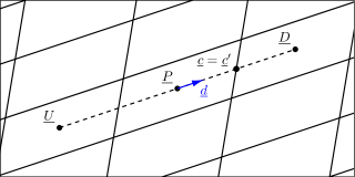
Figure 5: On a uniform structured grid, CUBISTA interpolates the value at face centre $\underline{c}$ from the values at the downwind ($D$), upwind ($P$), and farther-upwind ($U$) cells (assuming the mass flux is directed from cell $P$ to cell $D$).

So now we have a set of three co-linear and equidistant points, $\underline{U}$, $\underline{P}$ and $\underline{D}$, and three corresponding values, $\phi_{U}$, $\phi_{P}$ and $\phi_{D}$, and CUBISTA can be employed to calculate the value at point $\underline{c}^{\prime}_{f}$, which lies on the same line as these three points. Defining the normalised variables as

$$\xi\;=\;\frac{\|\underline{c}^{\prime}-\underline{P}\|}{\|\underline{D}-\underline{P}\|}$$ (52)

$$\tilde{\phi}_{P}\;=\;\frac{\phi_{P}-\phi_{U}}{\phi_{D}-\phi_{U}}$$ (53)

$$\tilde{\phi}_{c^{\prime}_{f}}(\xi,\tilde{\phi}_{P})\;=\;\frac{\bar{\phi}^{{}_{C}}_{c^{\prime}_{f}}-\phi_{U}}{\phi_{D}-\phi_{U}}$$ (54)

(note that $\xi$ is just the linear interpolation factor multiplying $\phi_{N_{f}}$ in Eq. (28)), CUBISTA blends Quadratic Upwind Interpolation (QUICK) and first-order upwinding (UDS) as follows:

$$\tilde{\phi}_{c^{\prime}_{f}}(\xi,\tilde{\phi}_{P})\;=\;\left\{\begin{array}[]{l l l}\tilde{\phi}_{P}&\quad\text{if }\tilde{\phi}_{P}\leq 0&\text{(UDS)}\\[5.69046pt] \frac{1}{3}(1+\xi)(3+\xi)\tilde{\phi}_{P}&\quad\text{if }0<\tilde{\phi}_{P}<\frac{3}{8}&\text{(Transition 1)}\\[5.69046pt] (1-\xi^{2})\tilde{\phi}_{P}\;+\;\frac{1}{2}\xi(1+\xi)&\quad\text{if }\frac{3}{8}<\tilde{\phi}_{P}\leq\frac{3}{4}&\text{(QUICK)}\\[5.69046pt] (1-\xi)^{2}\tilde{\phi}_{P}\;+\;\xi(2-\xi)&\quad\text{if }\frac{3}{4}<\tilde{\phi}_{P}\leq 1&\text{(Transition 2)}\\[5.69046pt] \tilde{\phi}_{P}&\quad\text{if }\tilde{\phi}_{P}>1&\text{(UDS)}\end{array}\right.$$ (55)

From $\tilde{\phi}_{c^{\prime}_{f}}$ the un-normalised value $\bar{\phi}^{{}_{C}}_{c^{\prime}_{f}}$ can be recovered via (54) for use in Eq. (50). However, the scheme can be conveniently reformulated in terms of un-normalised $\phi$ values using the median function [64] as:

$$\bar{\phi}^{{}_{C}*}_{c^{\prime}_{f}}\; =\;\text{median}\left(\quad\phi_{P},\quad\phi_{U}\,+\,\frac{(1+\xi)(3+\xi)}{3}(\phi_{P}-\phi_{U}),\quad\phi_{D}\,-\,(1-\xi)^{2}(\phi_{D}-\phi_{P})\quad\right)$$ (56)

$$\bar{\phi}^{{}_{C}}_{c^{\prime}_{f}}\; =\;\text{median}\left(\quad\phi_{P},\quad\bar{\phi}^{{}_{C}*}_{c^{\prime}_{f}},\quad\phi_{P}\,+\,\frac{\phi_{D}-\phi_{U}}{2}\xi\,+\,\frac{1}{2}(\phi_{D}-2\phi_{P}+\phi_{U})\xi^{2}\quad\right)$$ (57)

which also automatically sets $\bar{\phi}^{{}_{C}}_{c^{\prime}_{f}}=\phi_{P}$ (UDS) when $\phi_{D}=\phi_{U}$. The scheme (55) is based on QUICK, but switches to UDS when there is a local minimum or maximum at $\underline{P}$ ($\tilde{\phi}_{P}<0$ or $\tilde{\phi}_{P}>1$), which could indicate a spurious oscillation. The region $\tilde{\phi}_{P}\in[3/8,3/4]$, where the variation between the three values $\phi_{U}$, $\phi_{P}$ and $\phi_{D}$ is not far from linear, is considered to be “safe” and QUICK is applied unreservedly there. The upper bound of this region, which for non-uniform structured grids is given to be a $\xi$-dependent value in [58], is chosen here to be the fixed number $\tilde{\phi}_{P}=3/4$ based on the same criterion as in [58], namely the condition that the quadratic profile passing through the three points $\underline{U}$, $\underline{P}$ and $\underline{D}$ is monotonic (no overshoots / undershoots). In terms of normalised variables, this condition requires that $\tilde{\phi}_{c^{\prime}_{f}}(\xi,\tilde{\phi}_{P})$, as given by the QUICK branch of Eq. (55), increases monotonically towards the value 1 as $\xi\rightarrow 1$, which is ensured by the condition $\partial\tilde{\phi}_{c^{\prime}_{f}}(\xi,\tilde{\phi}_{P})/\partial\xi|_{\xi=1}\geq 0\Rightarrow\tilde{\phi}_{P}\leq 3/4$. We also note that, if CUBISTA achieves its goal of producing smooth $\phi$ distributions, then grid refinement, which brings the points $\underline{U}$, $\underline{P}$ and $\underline{D}$ closer together, will cause $\phi$ to vary more linearly in the neighbourhood of the three points, i.e. $\tilde{\phi}_{P}\rightarrow 0.5$ as the grid is refined. On fine grids, therefore, CUBISTA reduces to QUICK throughout the domain, except at local extrema of $\phi$.

Finally, one can notice an interpolated value $\bar{\underline{\underline{\tau}}}{}_{P}$ in the stress transformation terms in the right-hand side of Eq. (49). An obvious choice is to set $\bar{\underline{\underline{\tau}}}{}_{P}=\underline{\underline{\tau}}{}_{P}$, but it was found in [65] that using instead a weighted average of the stress at $P$ and its neighbours can mitigate the high-$\operatorname{\mathit{Wi}}$ problem. In the original scheme [65] the weighting was based on the mass fluxes through the cell’s faces. However, we noticed that this causes a noticeable accuracy degradation and instead used the following scheme (written here for 2D problems):

$$(\nabla_{h}^{q}\underline{u})^{\mathrm{T}}_{P}\cdot\bar{\underline{\underline{\tau}}}{}_{P}\;+\;\bar{\underline{\underline{\tau}}}{}_{P}\cdot\nabla_{h}^{q}\underline{u}_{P}\;=\;\left[\begin{array}[]{l}2\,\overline{\tau_{11,P}}\,\frac{\partial u_{1}}{\partial x_{1}}\>+\>2\,\tau_{12,P}\,\frac{\partial u_{1}}{\partial x_{2}}\\ \tau_{11,P}\frac{\partial u_{2}}{\partial x_{1}}\>+\>\overline{\tau_{12,P}}(\frac{\partial u_{1}}{\partial x_{1}}+\frac{\partial u_{2}}{\partial x_{2}})\>+\>\tau_{22,P}\frac{\partial u_{1}}{\partial x_{2}}\\ 2\,\overline{\tau_{22,P}}\frac{\partial u_{2}}{\partial x_{2}}\;+\;2\,\tau_{12,P}\frac{\partial u_{2}}{\partial x_{1}}\end{array}\right]\,\begin{array}[]{l}\text{\small{(1,1) component}}\\ \text{\small{(1,2) component}}\\ \text{\small{(2,2) component}}\end{array}$$ (58)

where the velocity derivatives are the components of $\nabla_{h}^{q}\underline{u}{}_{P}$ and

$$\overline{\tau_{ij,P}}\;=\;\frac{1}{D\,\Omega_{P}}\sum_{f=1}^{F}\bar{\tau}_{ij,c_{f}}^{{}_{C}}\,s_{f}\,(\underline{c}{}_{f}-\underline{P})\cdot\underline{n}{}_{f}$$ (59)

where $D$ = 2 or 3, for 2D or 3D problems, respectively. The interpolation scheme (59) is 2nd-order accurate (Appendix D). In the (1,2) component of (58), the middle term, although equal to zero in the limit of infinite grid fineness due to the continuity equation, has been retained for numerical stability. Compared to simply setting $\overline{\tau_{ij,P}}=\tau_{ij,P}$, this scheme was found, in the numerical tests of Sec. 5, to allow an increase of about 40% in the maximum solvable $\operatorname{\mathit{Wi}}$ number and to provide a slight increase of accuracy. At wall boundaries it was found that using linearly extrapolated stress values in (59) leads to convergence difficulties. Therefore, wall boundary values were omitted in the calculation, weighting the values at the remaining faces by their $s_{f}(\underline{c}_{f}-\underline{P})\cdot\underline{n}_{f}$ factors, i.e. by replacing $D\,\Omega_{P}$ in the denominator of (59) by

$$D\,\Omega_{P}^{\prime}\;=\;\sum_{f\notin\{W_{P}\}}s_{f}\left(\underline{c}_{f}-\underline{P}\right)\cdot\underline{n}_{f}\;=\;D\,\Omega_{P}\;-\;\sum_{f\in\{W_{P}\}}s_{f}\left(\underline{c}_{f}-\underline{P}\right)\cdot\underline{n}_{f}$$ (60)

where $\{W_{P}\}$ is the set of wall boundary faces of cell $P$. This is a 1st-order accurate interpolation.

In the simulations of Sec. 6 we did not encounter the high-$\operatorname{\mathit{Wi}}$ problem, but should it arise one can transform the constitutive equation in terms of a more weakly varying function of the stress tensor such as the logarithm of the conformation tensor [66, 67]. This has been applied to the Saramito model in [68].

3.5 Temporal discretisation scheme

The approximate time derivatives in the momentum and constitutive equations are calculated with a 2nd-order accurate, three-time level implicit scheme with variable time step. Suppose we enter time step $i$ and let $\phi_{P}^{i}$ be the current, yet unknown, value of $\phi$ at cell $P$. Fitting a quadratic Lagrange polynomial between the three points $(t_{i},\phi_{P}^{i})$, $(t_{i-1},\phi_{P}^{i-1})$ and $(t_{i-2},\phi_{P}^{i-2})$ and differentiating it at $t=t_{i}$ gives the following approximate time derivative:

$$\left.\frac{\mathrm{d}\phi}{\mathrm{d}t}\right|_{P}^{a}(t_{i})\;=\;l^{\prime}_{i,i}(t)\phi_{P}^{i}\;+\;l^{\prime}_{i,i-1}(t)\phi_{P}^{i-1}\;+\;l^{\prime}_{i,i-2}(t)\phi_{P}^{i-2}$$ (61)

where

$$l^{\prime}_{i,i}(t)=\frac{2t_{i}-t_{i-1}-t_{i-2}}{(t_{i}-t_{i-1})(t_{i}-t_{i-2})},\;\;l^{\prime}_{i,i-1}(t)=\frac{2t_{i}-t_{i}-t_{i-2}}{(t_{i-1}-t_{i})(t_{i-1}-t_{i-2})},\;\;l^{\prime}_{i,i-2}(t)=\frac{2t_{i}-t_{i}-t_{i-1}}{(t_{i-2}-t_{i})(t_{i-2}-t_{i-1})}$$ (62)

All other terms of the governing equations are evaluated at the current time (the scheme is fully implicit).

After solving the equations to obtain $\phi_{P}^{i}$ and deciding (as will be described shortly) the next time step size $\Delta t_{i+1}=t_{i+1}-t_{i}$, to facilitate the solution at the new time $t_{i+1}$ we can make a prediction by evaluating the aforementioned Lagrange polynomial at $t=t_{i+1}$ to obtain a provisional value $\phi_{P}^{i+1*}$. This value serves as an initial guess for solving the equations at the new time step $i+1$, offering significant acceleration. We perform such a prediction even for pressure, whose time derivative does not appear in the governing equations, as this was found to accelerate the solution of the continuity equation.

The subsequent solution at time $t_{i+1}$ will give us a value $\phi_{P}^{i+1}\neq\phi_{P}^{i+1*}$, in general. In order to obtain an estimate of the $O(h^{2})$ truncation error of scheme (61) we can augment our set of three points by the addition of the point $(t_{i+1},\phi_{P}^{i+1})$ and fit a cubic polynomial through the four points; the difference between $\partial\phi/\partial t|^{a}_{P}$ and $\partial\phi/\partial t|^{c}_{P}$, the derivatives predicted at time $t_{i}$ by the quadratic and cubic polynomials, respectively, is an approximation of the truncation error associated with $\partial\phi/\partial t|^{a}_{P}$. Omitting the details, it turns out that

$$\left.\frac{\partial\phi}{\partial t}\right|_{P}^{c}(t_{i})\;-\;\left.\frac{\partial\phi}{\partial t}\right|_{P}^{a}(t_{i})\;=\;c\,\frac{\phi_{P}^{i+1}-\phi_{P}^{i+1*}}{\Delta t_{i+1}}$$ (63)

where the factor $c=O(1)$ depends on the relative magnitudes of $\Delta t_{i-1}$, $\Delta t_{i}$ and $\Delta t_{i+1}$ ($c$ = 1/3 for $\Delta t_{i-1}=\Delta t_{i}=\Delta t_{i+1}$). This allows us to keep an approximately constant level of truncation error by adjusting the time step sizes so as to keep the right-hand side of Eq. (63) constant. We set the following goal, which accounts for all grid cells at once:

$$g_{t}^{i}\equiv\sqrt{\frac{1}{\Omega}\sum_{P}\Omega_{P}\left(\frac{\phi_{P}^{i}-\phi_{P}^{i*}}{\Delta t_{i}}\right)^{2}}\;=\;\tilde{g}^{0}_{t}\,\frac{\Phi}{T}$$ (64)

I.e. we want $g_{t}^{i}$, the $L_{2}$ norm of $(\phi_{P}^{i}-\phi_{P}^{i*})/\Delta t_{i}$, for any time step $i$, to equal a pre-selected non-dimensional target value $\tilde{g}_{t}^{0}$ times $\Phi/T$ where $\Phi$ is either $U$ (for the momentum equation, where $\phi\equiv u_{j}$) or $S$ (for the constitutive equation, where $\phi\equiv\tau_{jk}$). Suppose then that at some time step $i$ we are somewhat off target, i.e. Eq. (64) is not satisfied; we can try to amend this at the new time step $i+1$ by noting that the truncation error, and the associated metric $g_{t}$, are of order $O(\Delta t^{2})$, which means that $g_{t}^{i+1}/g_{t}^{i}=(\Delta t_{i+1}/\Delta t_{i})^{2}$. This relation allows us to choose $\Delta t_{i+1}$ so that $g_{t}^{i+1}$ will equal $\tilde{g}_{t}^{0}\Phi/T$ (Eq. (64)):

$$\Delta t_{i+1}\;=\;r_{t}^{i}\,\Delta t_{i}\qquad\text{where}\qquad r_{t}^{i}\;=\;\sqrt{\tilde{g}_{t}^{0}/\tilde{g}_{t}^{i}},\quad\tilde{g}_{t}^{i}\;=\;\frac{g_{t}^{i}}{\Phi/T}$$ (65)

In practice, we calculate the adjustment ratios $r_{t}^{i}$ for all variables whose time derivatives appear in the governing equations (one per velocity component and per stress component) and choose the smallest among them. We also limit the allowable values of $r_{t}^{i}$ to a range $r_{t}^{i}\in[r_{t}^{\min},r_{t}^{\max}]$, and also the overall time step size to $\Delta t_{i}\in[\Delta t_{\min},\Delta t_{\max}]$. Typical values used for these parameters in the simulations of Sec. 6 are $\tilde{g}_{t}^{0}$ = ${10}^{-4}$, $r_{t}^{\min}$ = $0.95$, $r_{t}^{\max}$ = $1.001$, $\Delta t_{\min}$ =$5\text{\times}{10}^{-5}$ $\mathrm{s}$, $\Delta t_{\max}$ = $2\text{\times}{10}^{-3}$ $\mathrm{s}$ (these may vary slightly between simulations). The scheme automatically chooses small time steps when the flow evolves rapidly, such as during the early stages of the flow, and large time steps when it evolves slowly, such as when the flow is nearing its steady state. A similar scheme is used in [69].

4 Solution of the algebraic system

Discretisation results in one large nonlinear algebraic system per time step. These systems are solved using the SIMPLE algorithm, with multigrid acceleration, where the algebraic equations are arranged into groups, one for each momentum and constitutive equation component, each of which through linearisation produces a linear system for one of the dependent variables. The algorithm is applied in the same manner as for viscoelastic flows [26, 28]; in each SIMPLE iteration, we solve successively: the linear systems for each stress component, the linear systems for the velocity components, and the pressure correction system to enforce continuity. The systems are solved with preconditioned conjugate gradient (pressure correction) or GMRES (all other variables) solvers.

In the velocity systems, derived from the components of the momentum eq. (40), the matrix of coefficients is constructed via a contribution from the time derivative, a UDS discretisation of the convective term, and the $D_{f,i}^{\tau+}$ (Eq. (42)) part of the EVP force $\underline{F}_{f}^{\tau}$. The remaining terms are evaluated from their currently estimated values and moved to the right-hand side vector, as is the difference between the UDS and CDS convection schemes (deferred correction). For the stress systems we follow the established practice in viscoelastic flows of constructing the matrix of coefficients with contributions only from the terms of the left-hand side of Eq. (49), breaking the CUBISTA flux into a UDS component and a remainder which is moved to the right-hand side vector (deferred correction). This poor representation of the constitutive equation by the matrix of coefficients may be responsible for the observed convergence difficulties of SIMPLE at large time steps; for small time steps the role of the time derivative in the constitutive equation becomes dominant and convergence is fast.

It was noticed that if the residual reduction within each time step is not at least a couple orders of magnitude, then the temporal prediction step (Sec. 3.5) may not produce good enough initial guesses and the solution may not be smooth in time. To avoid this possibility we set a maximum effort per time step of about 20 single-grid SIMPLE iterations followed by about 5 W(4,4) multigrid cycles [70, 24], and if further iterations are needed to accomplish the required residual reduction then the time step is reduced by a factor of $r_{t}^{\min}$ (Sec. 3.5). Setting $\Delta t_{\max}$ to an appropriate value avoids the need for this.

5 Validation and testing of the method in Oldroyd-B flow

For $\tau_{y}=0$ and $n=1$, the SHB model reduces to the Oldroyd-B viscoelastic model, for which benchmark results for square lid-driven cavity flow can be found in the literature. We apply our method to this problem to validate it and to evaluate alternative options for the FVM components. The problem is solved as steady-state, omitting the time derivatives from the governing equations. Table 1 lists the computed location and strength of the main vortex, along with values reported in the literature, with which there is very good agreement.

Table 1: $\tilde{x}-$ and $\tilde{y}-$ coordinates $(\tilde{x}_{c},\tilde{y}_{c})$ of the centre of the main vortex for Oldroyd-B flow in a square cavity of side $L$, and associated value of the streamfunction there, $\tilde{\psi}_{c}$. The top wall moves in the positive $x-$direction with variable velocity $u(x)=16U(x/L)^{2}(1-x/L)^{2}$. The coordinates are normalised by the cavity side $L$ and the streamfunction by $UL$. The flow is steady, the Reynolds number is zero, and the solvent and polymeric viscosities are equal ($\kappa=k$).

	$\operatorname{\mathit{Wi}}=0.5$			$\operatorname{\mathit{Wi}}=1.0$
	$\tilde{x}_{c}$	$\tilde{y}_{c}$	$\tilde{\psi}_{c}$	$\tilde{x}_{c}$	$\tilde{y}_{c}$	$\tilde{\psi}_{c}$
Pan et al. [71]	$0.469$	$0.798$	$-0.0700$	$0.439$	$0.816$	$-0.0638$
Saramito [72]				$0.429$	$0.818$	$-0.0619$
Sousa et al. [35]	$0.467$	$0.801$	$-0.0698$	$0.434$	$0.814$	$-0.0619$
Zhou et al. [65]	$0.468$	$0.798$		$0.430$	$0.818$
Present results	$0.468$	$0.799$	$-0.0698$	$0.434$	$0.818$	$-0.0619$

To estimate discretisation errors, we obtained accurate estimates of the $\operatorname{\mathit{Wi}}=0.5$ and $\operatorname{\mathit{Wi}}=1.0$ solutions by Richardson extrapolation of the solutions obtained on uniform Cartesian grids (Fig. 6(a)) of $512\times 512$ and $1024\times 1024$ cells; the procedure is described in detail in [53]. These extrapolated solutions served as “exact” solutions against which we calculated the discretisation errors of coarser grids. Figure 7 plots average velocity and stress discretisation errors defined as

$$\epsilon_{u}\;\equiv\;\frac{1}{\#\Omega^{\prime}}\sum_{P\in\Omega^{\prime}}\|\underline{u}^{e}_{P}-\underline{u}_{P}\|\;/\;\|\underline{u}^{e}\|_{\mathrm{avg}}$$ (66)

$$\epsilon_{\tau}\;\equiv\;\frac{1}{\#\Omega^{\prime}}\sum_{P\in\Omega^{\prime}}\|\underline{\underline{\tau}}^{e}_{P}-\underline{\underline{\tau}}_{P}\|\;/\;\|\underline{\underline{\tau}}^{e}\|_{\mathrm{avg}}$$ (67)

where the superscript $e$ denotes the “exact” solution, calculated by Richardson extrapolation. The summation is over all cells $P$ whose centres lie inside the area $\Omega^{\prime}=[0.05L,0.95L]\times[0.05L,0.95L]$ ($\#\Omega^{\prime}$ is the total number of such cells), $L$ being the cavity length, i.e. a strip of width $0.05L$ touching the boundary is excluded, because the stress magnitude ($\tau_{xx}$ in particular) appears to grow exponentially over part of the top boundary and this inflates the discretisation errors there. The vector and tensor magnitudes in (66) and (67) are $\|\underline{u}\|=(\sum_{i}u_{i}^{2})^{1/2}$ and $\|\underline{\underline{\tau}}\|=(\sum_{ij}\tau_{ij}^{2})^{1/2}$. The definitions (66) and (67) incorporate a normalisation of the errors by the average velocity and stress magnitudes over $\Omega^{\prime}$: $\|\underline{u}^{e}\|_{\mathrm{avg}}\equiv(1/\Omega^{\prime})\int_{\Omega^{\prime}}\|\underline{u}^{e}\|\mathrm{d}\Omega$ and $\|\underline{\underline{\tau}}^{e}\|_{\mathrm{avg}}\equiv(1/\Omega^{\prime})\int_{\Omega^{\prime}}\|\underline{\underline{\tau}}^{e}\|\mathrm{d}\Omega$. In Fig.  7 the discretisation errors are plotted with respect to the average grid spacing $h=(\Omega/\#\Omega)^{1/2}$ which equals $L/N$ for a $N\times N$ grid of any of the kinds shown in Fig. 6.

To ensure that our method is applicable to unstructured grids, although the geometry favours discretisation by uniform (Fig. 6(a), “CU”) or non-uniform (Fig. 6(b), “CN”) Cartesian grids, we also employed grids obtained from the CU ones by randomly perturbing their vertices as described in [44]. In particular, from a $N\times N$ CU grid (Fig. 6(a)) a $N\times N$ distorted grid is constructed (Fig. 6(c)) by moving each interior node $(x,y)$ to a location $(x^{\prime},y^{\prime})=(x+\delta x,y+\delta y)$ where $\delta x$ and $\delta y$ are randomly selected for each node under the restriction that $|\delta x|,|\delta y|<h/4$. This restriction ensures that all resulting grid cells are simple convex quadrilaterals. This procedure produces a series of grids whose skewness, unevenness and non-orthogonality do not diminish with refinement [44], as is typical of unstructured grids. Checking the convergence of the method on this sort of grids is important because in [44] it was shown that there are popular FVM discretisations, widely regarded as second-order accurate, which actually do not converge to the exact solution with refinement on unstructured grids. So, we employed three series of grids, one for each of the grid types shown in Fig. 6, having $32\times 32$, $64\times 64$, $128\times 128$, $256\times 256$ and $512\times 512$ cells. The CN grids were constructed as follows: in the $512\times 512$ such grid, the grid spacing at the walls equals $L/1024$ and grows under a constant ratio towards the cavity centre. Then, by removing every second grid line we obtain the $256\times 256$ grid, and so on for coarser grids.

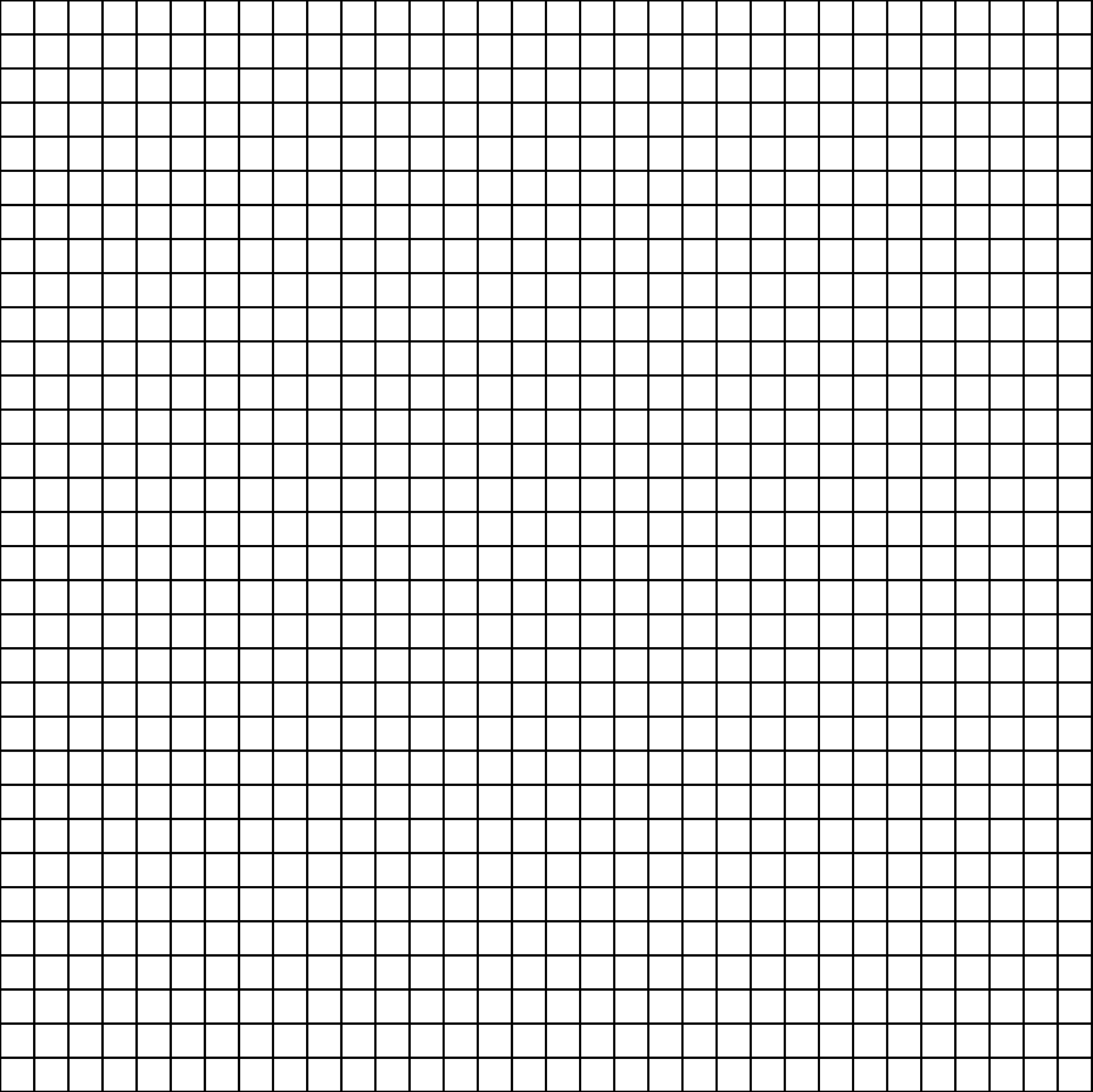
(a) Cartesian uniform (CU)

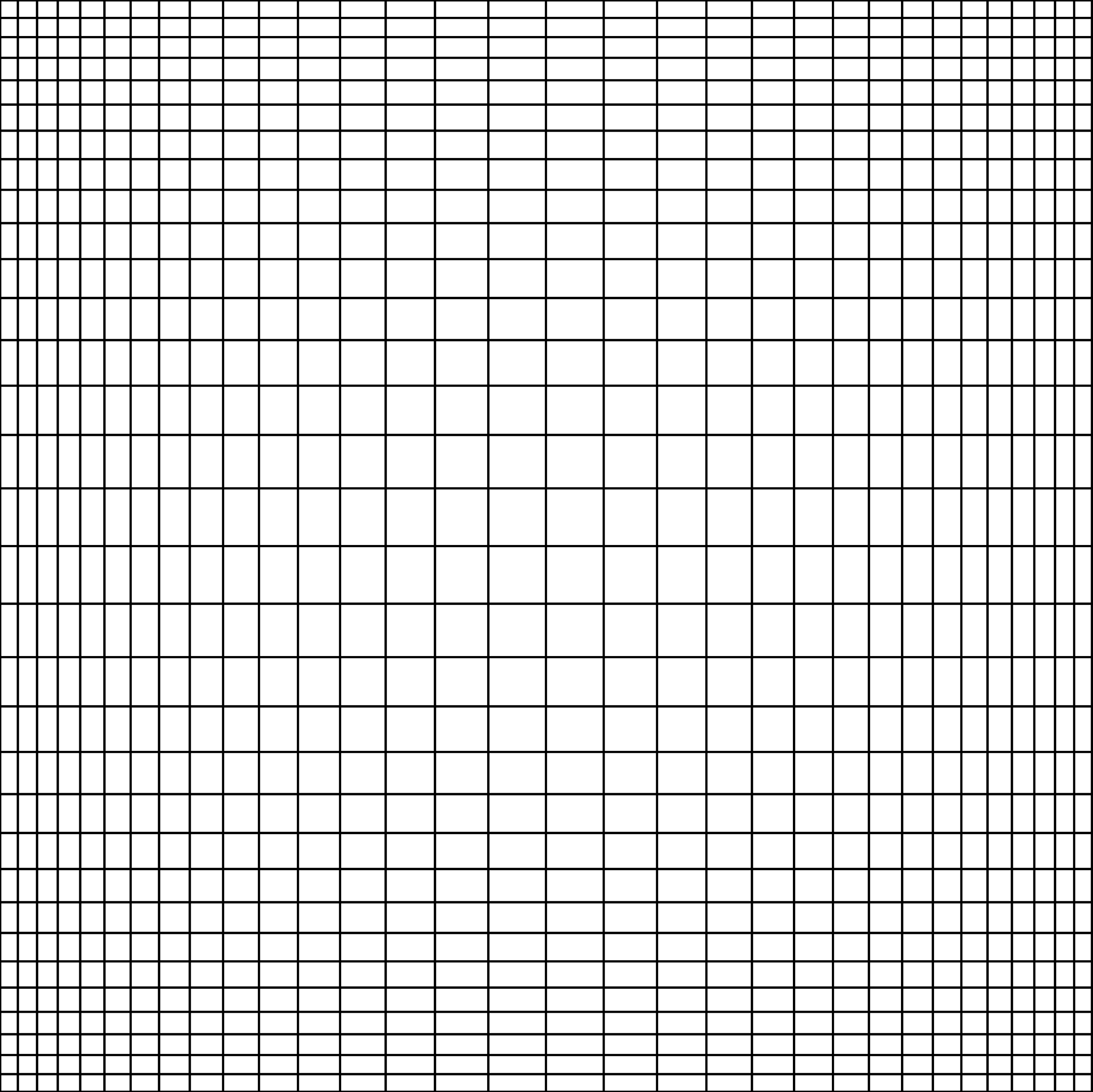
(b) Cartesian non-uniform (CN)

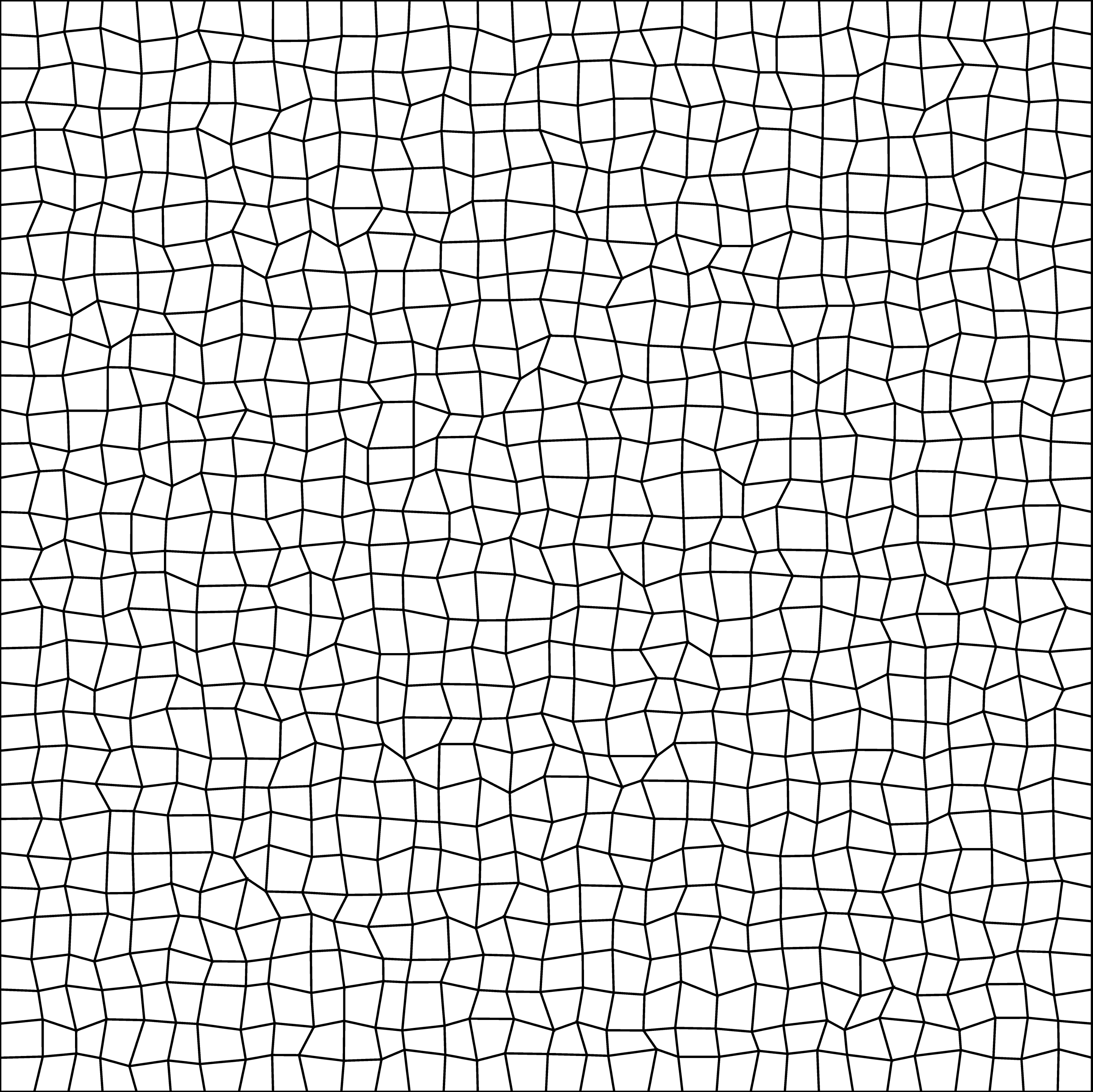
(c) Distorted (D)

Figure 6: $32\times 32$ grids of different kinds, used for the Oldroyd-B benchmark problems.

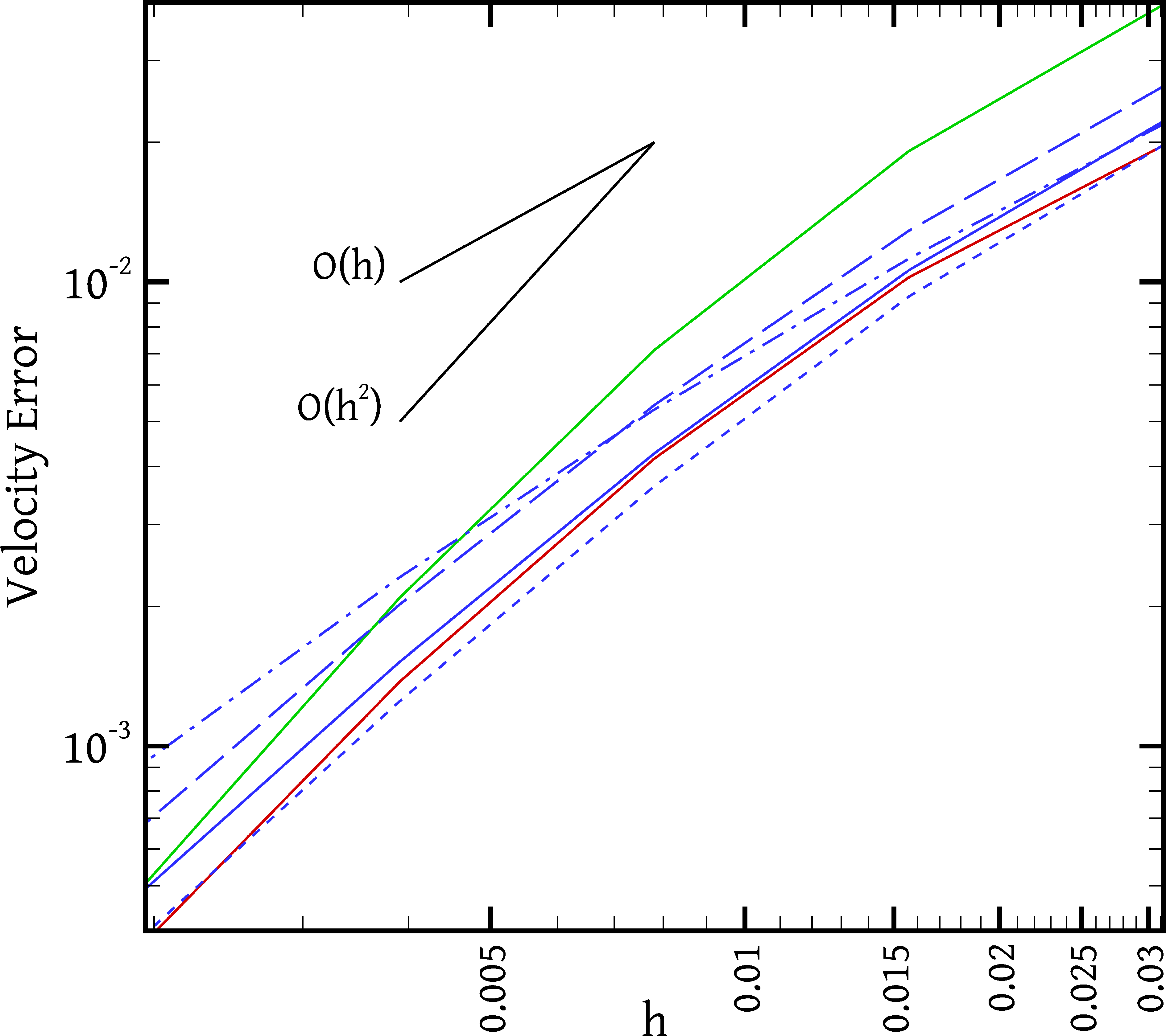
(a) $\operatorname{\mathit{Wi}}=0.5$, CU grids: $\epsilon_{u}$

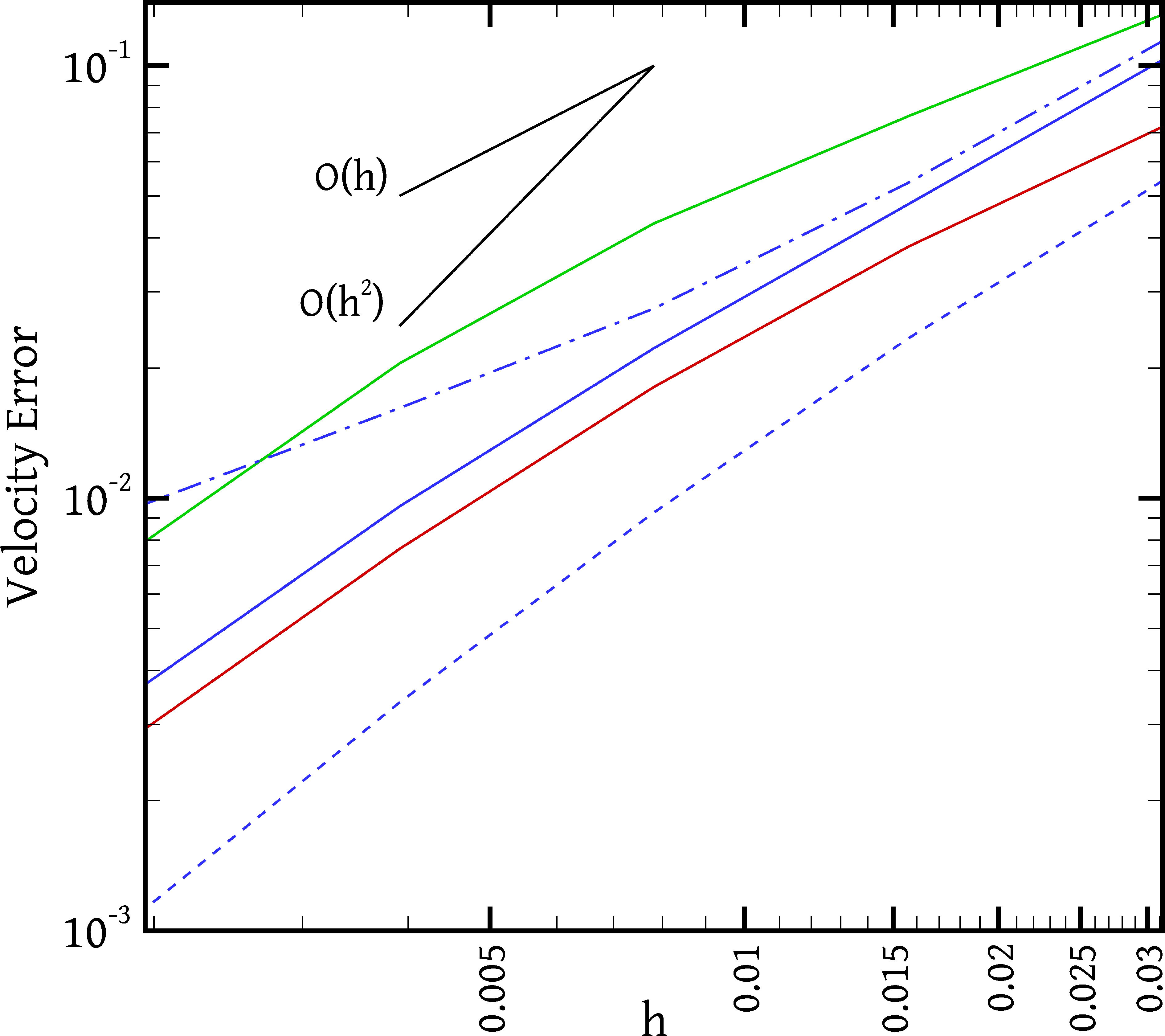
(b) $\operatorname{\mathit{Wi}}=1.0$: $\epsilon_{u}$

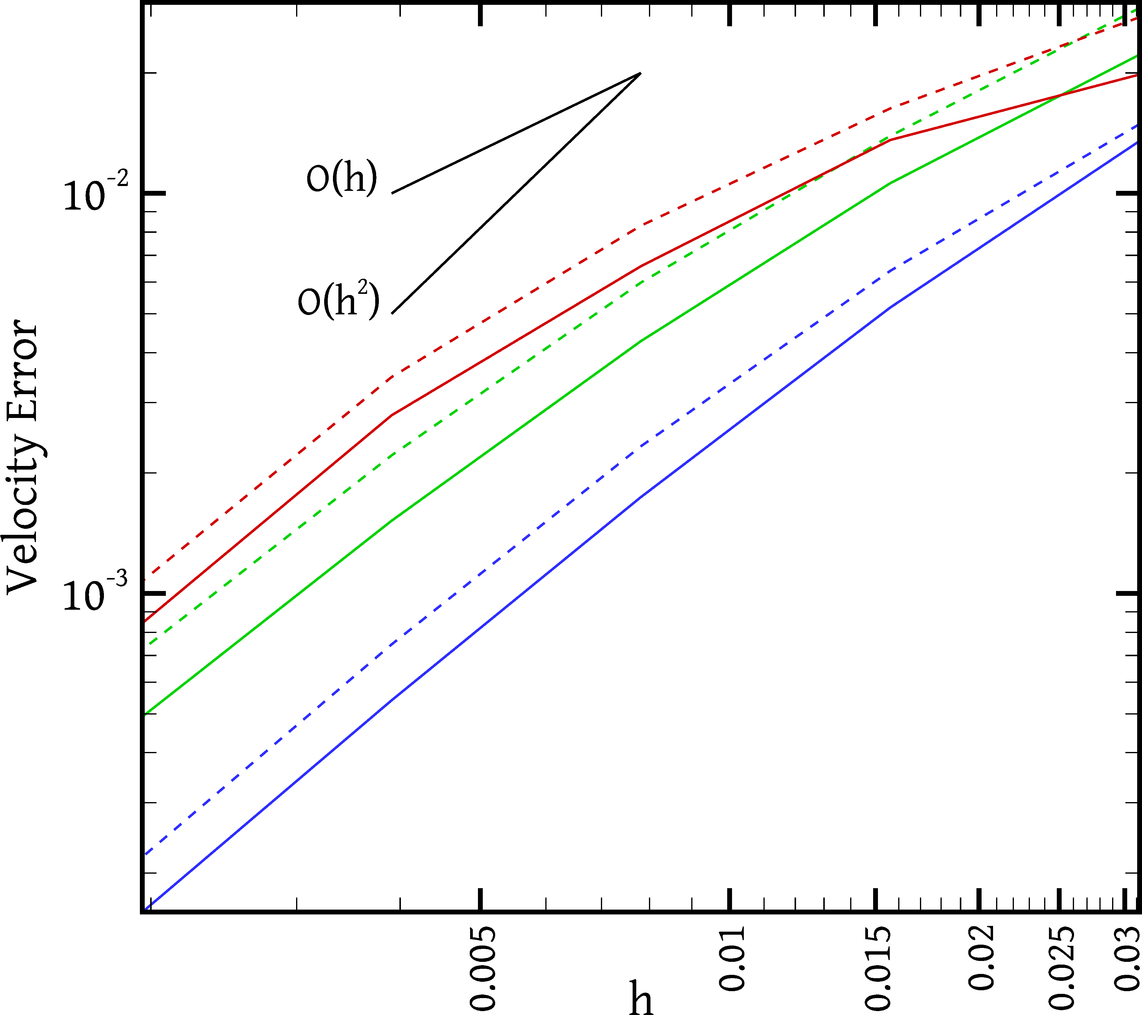
(c) $\operatorname{\mathit{Wi}}=0.5$; CU,CN,D grids: $\epsilon_{u}$

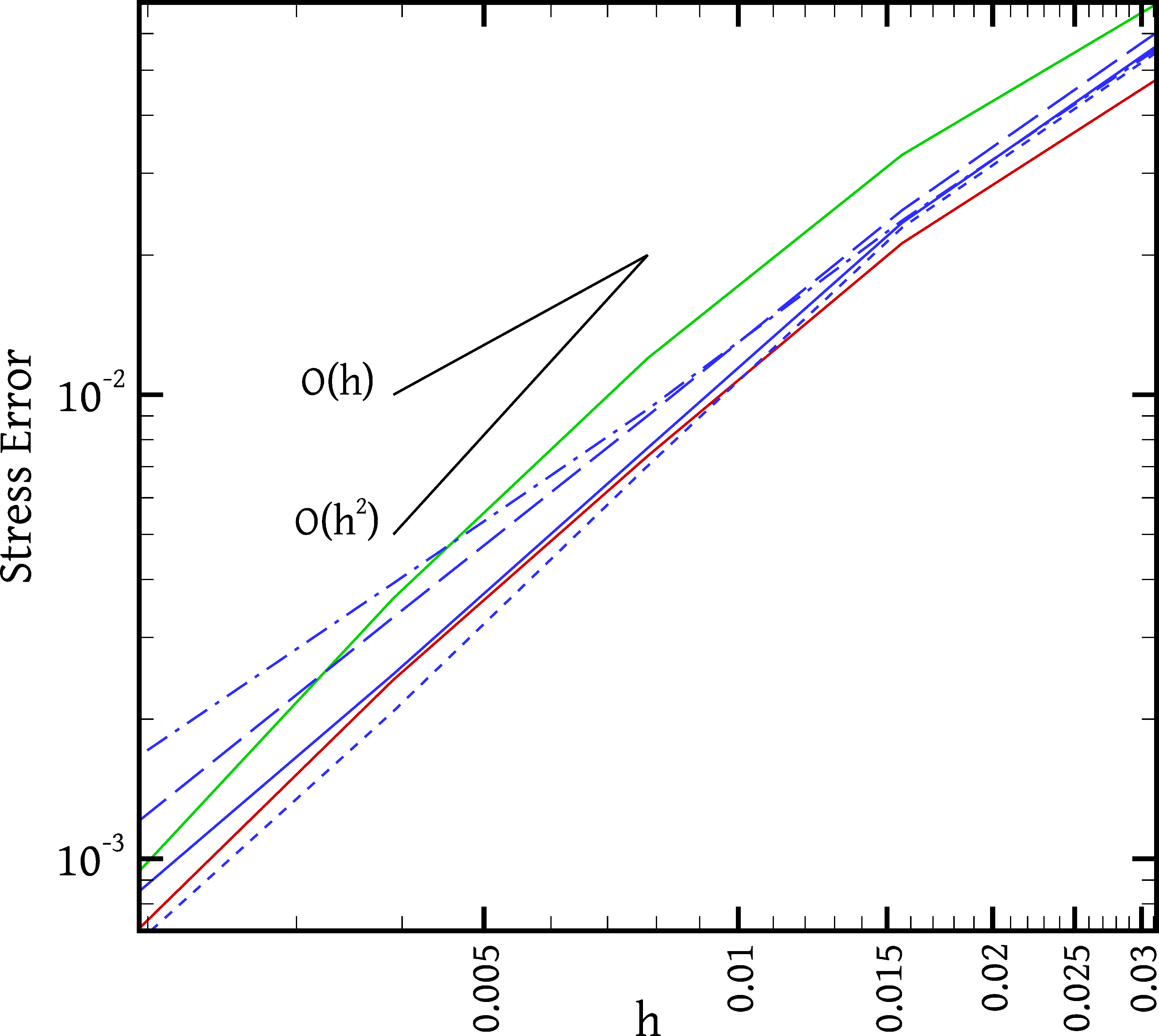
(d) $\operatorname{\mathit{Wi}}=0.5$, CU grids: $\epsilon_{\tau}$

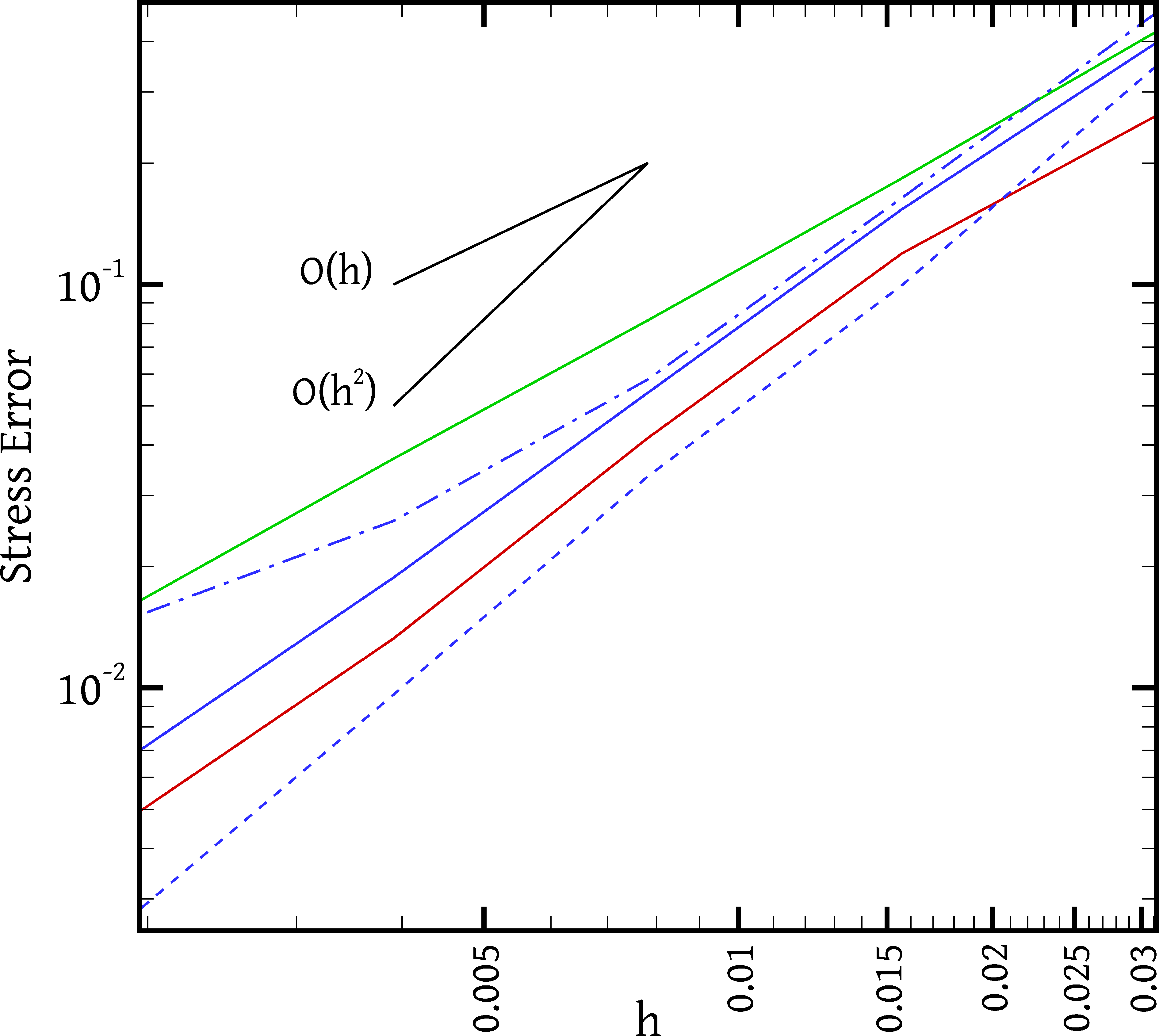
(e) $\operatorname{\mathit{Wi}}=1.0$: $\epsilon_{\tau}$

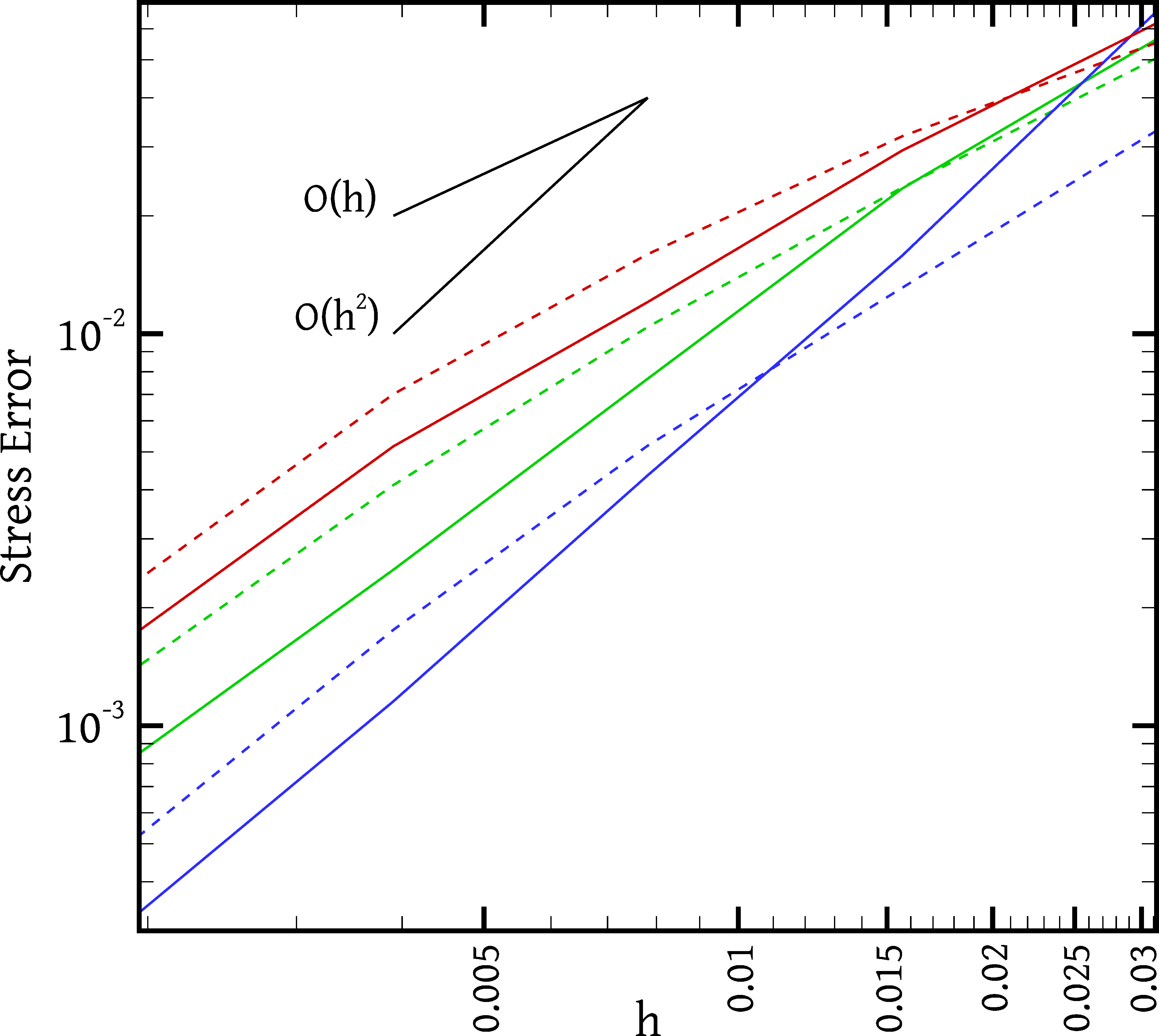
(f) $\operatorname{\mathit{Wi}}=0.5$; CU,CN,D grids: $\epsilon_{\tau}$

Figure 7: Velocity (top row) and stress (bottom row) discretisation errors (Eqs. (66) and (67)) of Oldroyd-B flow as a function of the grid spacing $h$, for various cases. Unless otherwise stated, the $\nabla_{h}^{1.5}$ gradient is used and the $D$’s at boundary faces are given by (46) – (47). Figs. 7(a), 7(d): $\operatorname{\mathit{Wi}}=0.5$, CU grids (Fig. 6(a)). Green, red and blue lines correspond to setting $\overline{\tau_{ij,P}}=\tau_{ij,P}$ in (58), using the log-conformation technique, and defining $\overline{\tau_{ij,P}}$ by (59) in (58), respectively. In the latter case, the solid and dash-dot lines correspond to the use of Eqs. (25) and (26), respectively. Dashed lines with short or long dashes correspond, respectively, to replacing $S$ by $S/2$ or $2S$ in (25). Figs. 7(b), 7(e): as for Figs. 7(a), 7(d), but for $\operatorname{\mathit{Wi}}=1.0$. The dashed line now corresponds to CN grids (Fig. 6(b)), using (25) and (12). Figs. 7(c), 7(f): $\operatorname{\mathit{Wi}}=0.5$, use of (25) and (12). Green, blue, and red lines: CU (Fig. 6(a)), CN (Fig. 6(b)), and D (Fig. 6(c)) grids, respectively. Dashed lines correspond to use of $\nabla^{1.0}_{h}$ and simple linear extrapolation of stresses to the walls (i.e. setting $D_{b,i}^{\tau+}=D_{b,i}^{\tau-}=0$ instead of (46) – (47)).

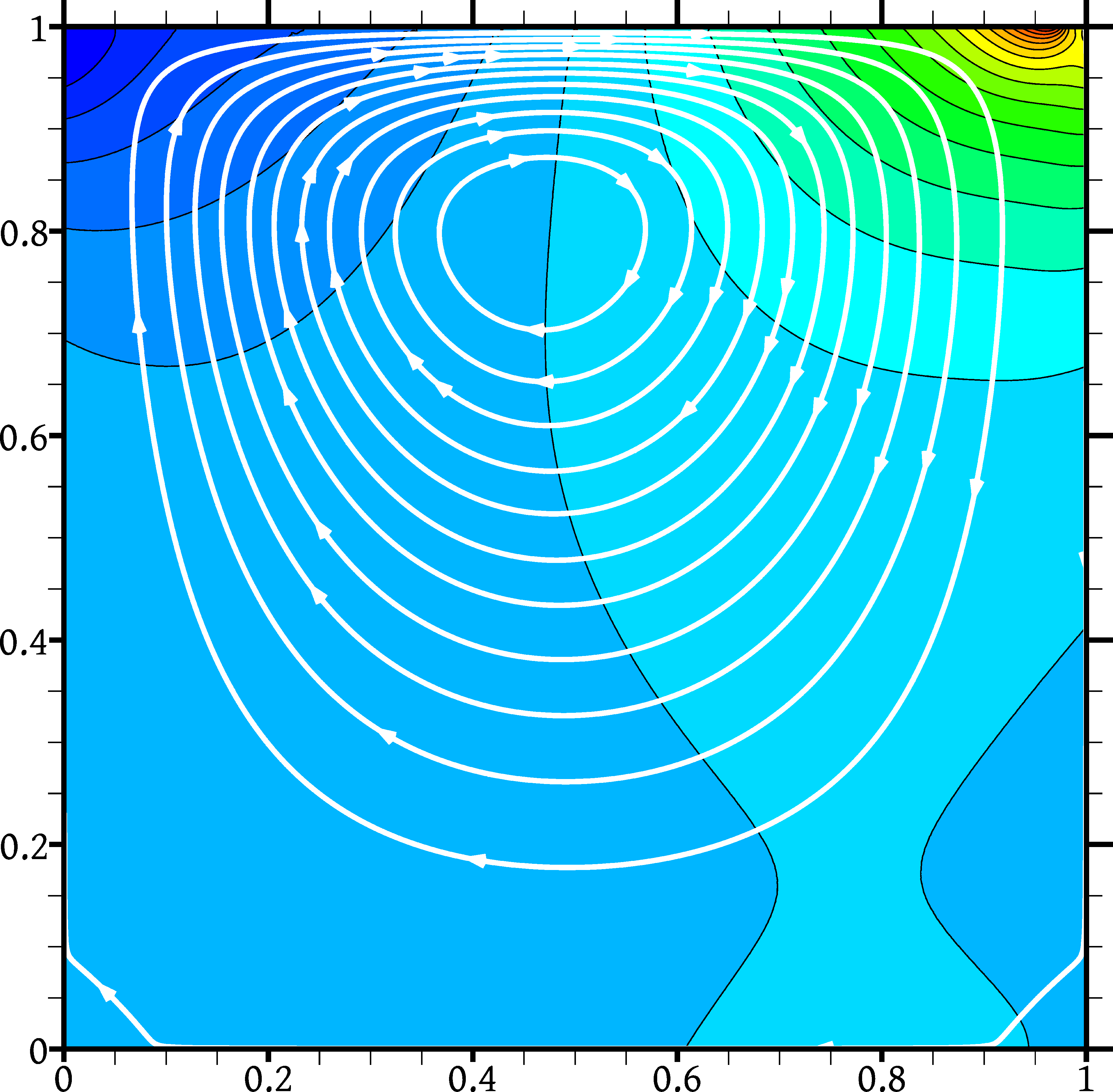
(a) Pressure

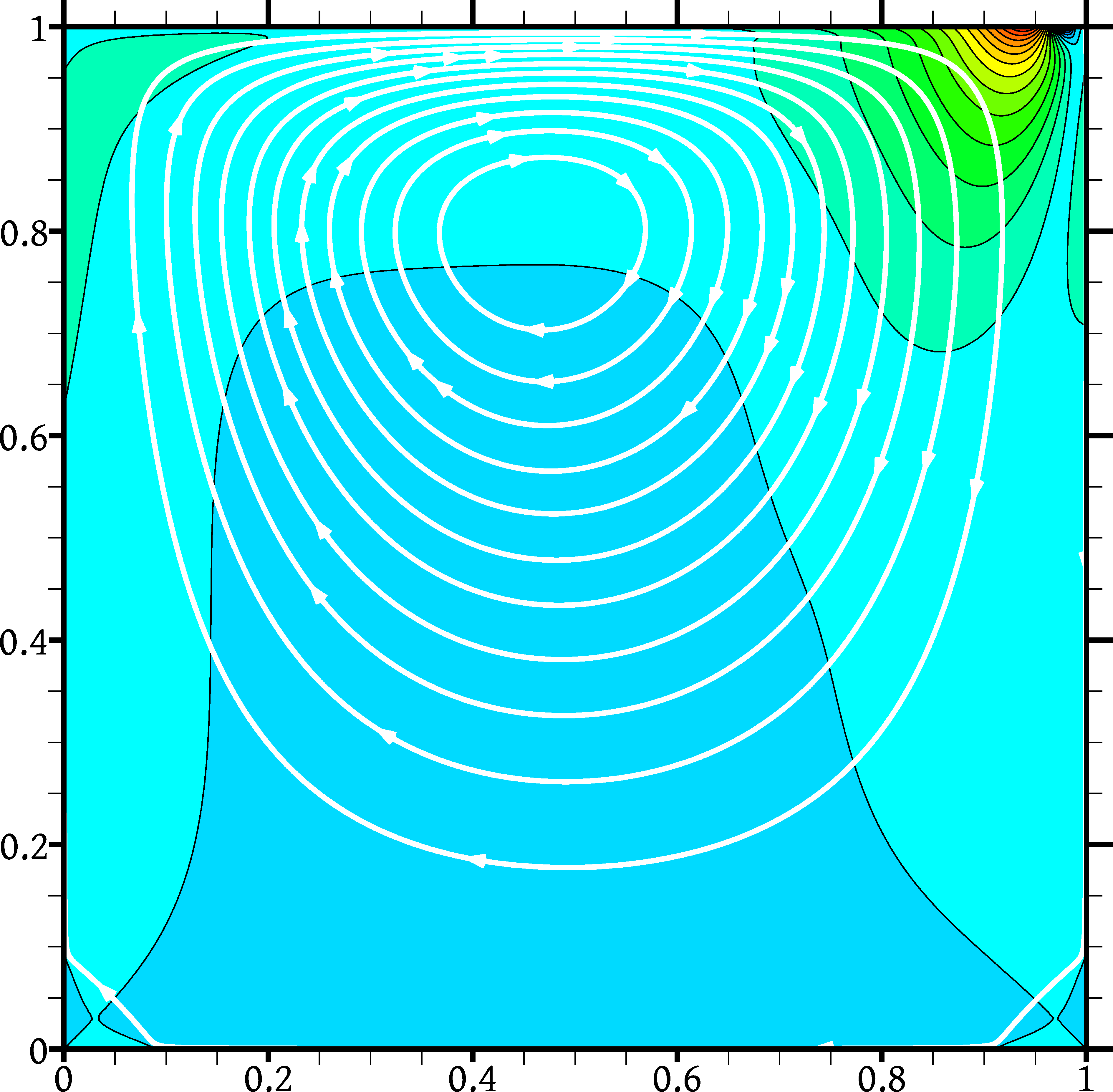
(b) Stress $\tau_{12}$

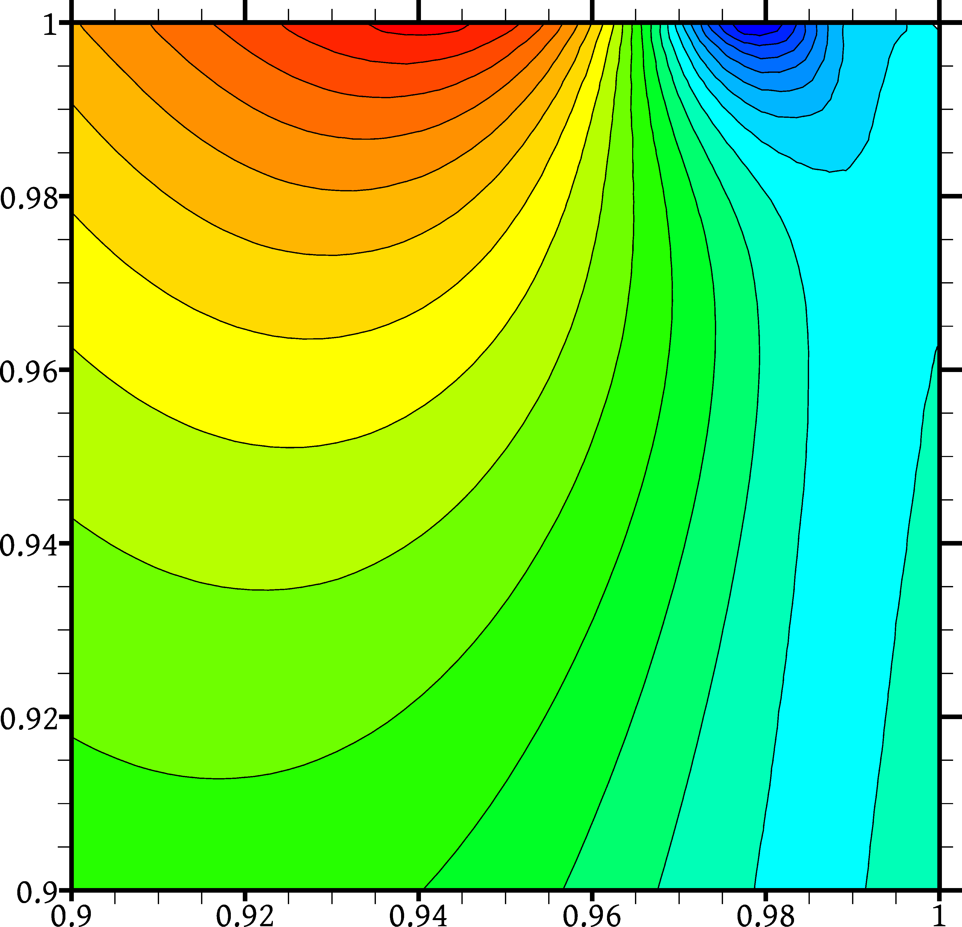
(c) Stress $\tau_{12}$

Figure 8: The Oldroyd-B, $\operatorname{\mathit{Wi}}=0.5$ flow field calculated on the $512\times 512$ distorted grid. 8(a) Pressure contours (colour, $\delta p=4S$ with $S$ given by Eq. (12)) and streamlines (white lines). 8(b) Contours of $\tau_{12}$ ($\delta\tau_{12}=2S$) and streamlines. 8(c) Close-up view of 8(b) near the upper-right corner.

The numerical tests led to the following observations. Concerning the oscillations issue, the stabilisation strategies achieved their goal as all dependent variables varied smoothly across the domain without spurious oscillations; Fig. 8 shows smooth pressure and $\tau_{12}$ fields and streamlines obtained on the $512\times 512$ distorted grid. Concerning the accuracy of the method, Fig. 7 shows convergence to the exact solution with grid refinement on any type of grid, including the randomly distorted type. The order of accuracy is close to 1 on coarse grids and increases towards 2 (the design value) as the grid is refined, but for the $\operatorname{\mathit{Wi}}=1$ case (Figs. 7(b), 7(e)) it is still quite far from 2 even on the finest ($512\times 512$) grids. Evidently, the convergence rates deteriorate at higher elasticity (compare Figs. 7(a),7(d) and 7(b),7(e)). The substandard accuracy performance of the method at high elasticity is most likely associated with the exponential stress growth near the lid. The Oldroyd-B predictions can be unrealistic, such as predicting unlimited extension of the material at finite extension rates; in such cases the accuracy of numerical methods can degrade significantly [73]. The SHB model suffers from these same issues as the Oldroyd-B model for $n\geq 1$, but not for $n<1$ [31].

With typical EVP materials it is usually the case that $\operatorname{\mathit{Wi}}<1$, which, combined with the fact that their behaviour is described by $n<1$, avoids the “high-$\operatorname{\mathit{Wi}}$” problem. Nevertheless, in the tests of the present Section we also tried the log-conformation technique [66, 67] which is implemented as an option in our code [29], and, interestingly, Fig. 7 shows that it can be beneficial even at low $\operatorname{\mathit{Wi}}$ as it provides enhanced accuracy. Interpolation (59) also appears to improve the accuracy compared to simply setting $\overline{\tau_{ij,P}}=\tau_{ij,P}$, although rate of convergence of the latter method appears to be higher for $\operatorname{\mathit{Wi}}=0.5$ so that it is expected to surpass the accuracy of interpolation (59) on even finer grids. Use of (59) was observed to enable obtaining a solution at slightly higher $\operatorname{\mathit{Wi}}$ compared to setting $\overline{\tau_{ij,P}}=\tau_{ij,P}$ (up to $\operatorname{\mathit{Wi}}\approx 1.4$ compared to $\operatorname{\mathit{Wi}}=1$). For the main results of Sec. 6 the scheme (59) was selected, given also that it is cheaper than the log-conformation method.

The scheme (26) performs poorly in terms of accuracy (Figs. 7(a),7(d) and 7(b),7(e), dash-dot lines) compared to the simpler scheme (25). Concerning the latter, it is noteworthy that the larger the value of $\eta_{a}$ (adjusted by replacing $S$ with larger / smaller values in (25)) the less accurate the results (Figs. 7(a),7(d), lines with long or short dashes). Thus, stabilisation should be exercised with parsimony. Henceforth we abandon the scheme (26) and employ scheme (25).

Fig. 7 shows that packing the grid lines close to the walls – i.e. using the CN grids – achieves a very significant increase of accuracy. This is likely related to the aforementioned singular behaviour near the lid. As expected, the discretisation errors are largest on the distorted grids (Figs. 7(c),7(f), red lines), but not by a great margin compared to the uniform Cartesian grids. The rates of error convergence towards zero are similar on all grid types. Another disadvantage of the distorted grids is that the high-$\operatorname{\mathit{Wi}}$ problem is intensified: for $\operatorname{\mathit{Wi}}=1$, we only managed to obtain a solution up to grid $64\times 64$ with the scheme (25), and up to grid $128\times 128$ with the scheme (26). Finally, we note that Figs. 7(c),7(f) show that the stress extrapolation scheme at the boundaries which uses (46) – (47), in combination with the gradient $\nabla_{h}^{1.5}$, which retains 2nd-order accuracy at the boundaries unlike the more popular $\nabla_{h}^{1}$ [44], leads to a noticeable accuracy improvement compared to simple linear extrapolation of stresses.

6 EVP flow in a lid-driven cavity

We now turn our attention to EVP flow in a lid-driven cavity. The SHB model parameters were chosen so as to represent the behaviour of Carbopol. Carbopol gels are used very frequently as prototypical viscoplastic fluids in experimental studies [11, 74]. In [33], the SHB model was fitted to experimental data for a Carbopol gel of concentration 0.2% in weight, and we rounded those parameters to arrive at our own chosen parameters, listed in Table 2. This material has a yield strain (Eq. (22)) of $\gamma_{y}=0.175$. It is enclosed in a square cavity of side $L$ = 0.1 $\mathrm{m}$ and the flow is driven by horizontal motion of the top wall (lid) towards the right. We employed a grid of $384\times 384$ cells, of uniform size in the $x$ direction but packed near the lid so that the vertical size of the cells touching the lid is $L/625$, and of those touching the bottom wall is about $L/252$. A coarse $48\times 48$ grid of similar packing is shown in Fig. 9.

Table 2: Properties of the fluid used in the EVP lid-driven cavity simulations.

$\rho$	1000	$\mathrm{k}\mathrm{g}\mathrm{/}\mathrm{m}^{3}$
$\tau_{y}$	70	$\mathrm{P}\mathrm{a}$
$G$	400	$\mathrm{P}\mathrm{a}$
$k$	20	$\mathrm{P}\mathrm{a}\,\mathrm{s}^{n}$
$n$	0.40

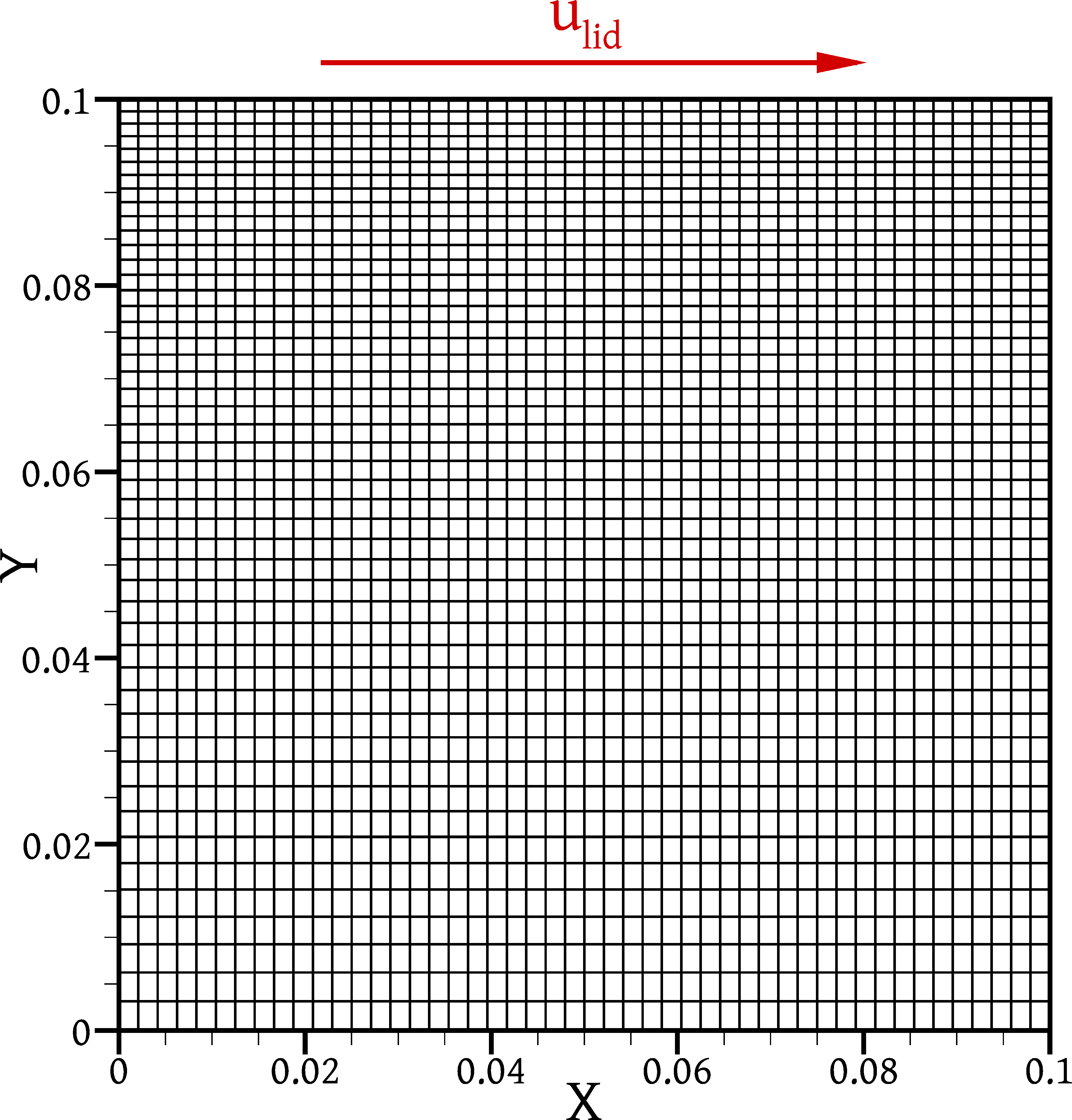
Figure 9: A coarse, $48\times 48$ cell grid, showing the packing of the cells near the lid (a coarse grid is shown for clarity; the EVP lid-driven cavity simulations were performed on a similar grid of $384\times 384$ cells).

6.1 The base case

We start with a case where the enclosed material is initially at rest and fully relaxed ($\underline{\underline{\tau}}=0$ everywhere). Starting from rest, the lid accelerates towards the right until it reaches a maximum velocity of $U$ = 0.1 $\mathrm{m}\mathrm{/}\mathrm{s}$ at time $T=L/U$ = 1 $\mathrm{s}$. The lid velocity remains constant thereafter:

$$u_{\mathrm{lid}}\;=\;U\sin\left(\frac{\min(t,T)}{T}\,\frac{\pi}{2}\right)$$ (68)

The dimensionless numbers for this case are listed in the “$U$ = 0.100 $\mathrm{m}\mathrm{/}\mathrm{s}$” column of Table 3.

Table 3: Values of the dimensionless numbers, and of the relaxation time (21), at different lid velocities.

$U$ [$\mathrm{m}\mathrm{/}\mathrm{s}$]	0.025	0.100	0.400
$\operatorname{\mathit{Bn}}^{\prime}$	6.094	3.500	2.010
$\operatorname{\mathit{Bn}}$	0.859	0.778	0.668
$\operatorname{\mathit{Wi}}$	0.204	0.225	0.262
$\operatorname{\mathit{Re}}$	0.008	0.111	1.526
$\lambda$ [$\mathrm{s}$]	0.815	0.255	0.066

Figure 10 shows the evolution in time of the normalised kinetic energy of the fluid and of the normalised average absolute value of the trace of the stress tensor, calculated as

$$\mathrm{N.K.E.}\;=\;\frac{1}{U^{2}\,\Omega}\sum_{P}\Omega_{P}\|\underline{u}_{P}\|^{2}$$ (69)

$$\mathrm{tr}(\underline{\underline{\tilde{\tau}}})_{\mathrm{avg}}\;=\;\frac{1}{S\,\Omega}\sum_{P}\Omega_{P}|\mathrm{tr}(\underline{\underline{\tau}}\!{}_{P})|$$ (70)

where $\Omega=L^{2}$ is the volume of the cavity. It is immediately obvious from Fig. 10 that the kinetic energy assumes a constant value very quickly, but the average stress trace evolves much more slowly. To investigate this, the simulation was carried on until a time of $t$ = 210 $\mathrm{s}$.

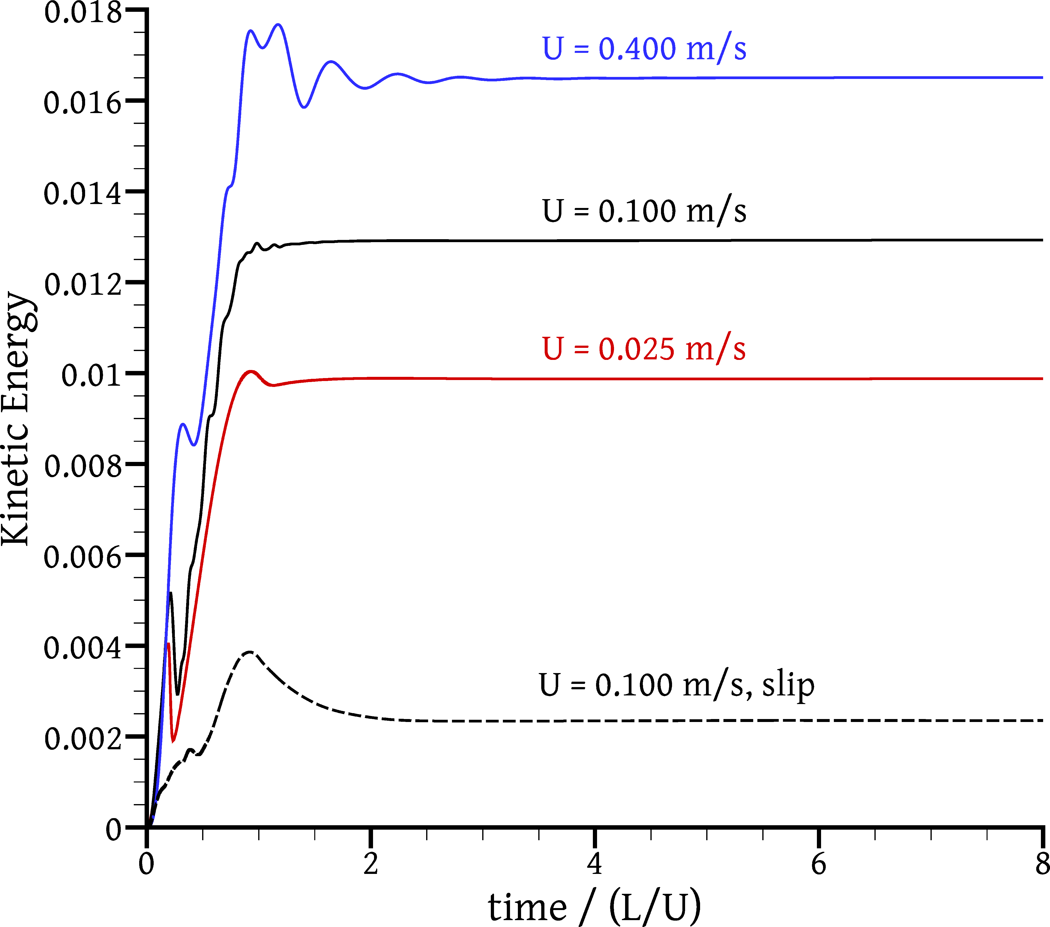
(a) N.K.E.

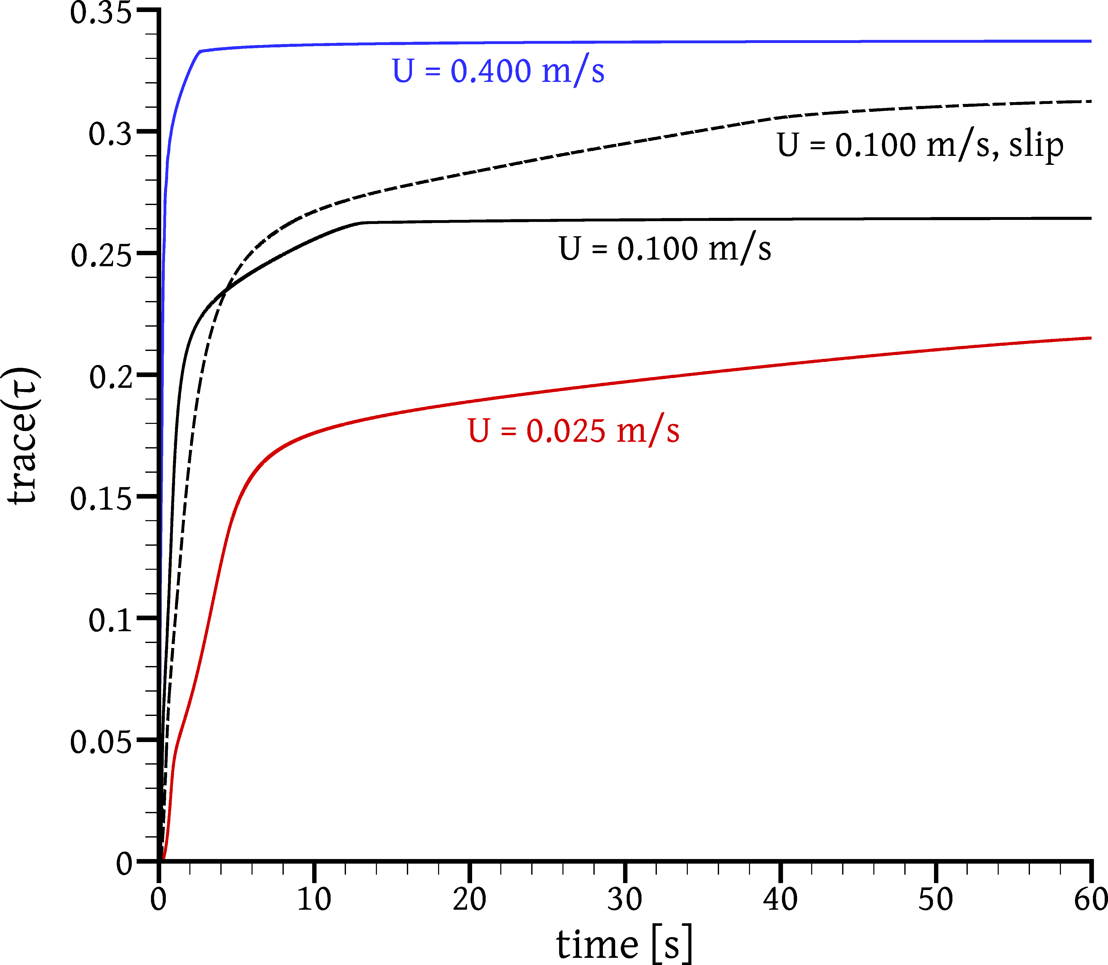
(b) $\mathrm{tr}(\underline{\underline{\tilde{\tau}}})_{\mathrm{avg}}$

Figure 10: 10(a) Normalised kinetic energy (Eq. (69)) and 10(b) normalised average trace of $\underline{\underline{\tau}}$ (Eq. (70)), versus time, for different lid velocities. In 10(a) time is normalised by $L/U$.

The flow field is visualised in Fig. 11. It resembles that for pure viscoplastic flow [24, 34], in that there are two unyielded zones ($\tau_{d}<\tau_{y}$), one at the bottom of the cavity touching the walls, containing stationary fluid, and one near the lid which is rotating with the flow and does not touch the walls, called a plug zone. Whether the material at a point is in a yielded or unyielded state is, of course, determined by whether $\tau_{d}$ is larger or smaller, respectively, than the yield stress $\tau_{y}$ there (Eq. (7)). Figure 11(b) shows that the streamlines do not cross into the lower unyielded zone, which therefore always consists of the same material, but they cross into and out of the plug zone. Thus, at every instant in time, liquefied particles are entering the plug zone, solidifying upon entry, while other, solidified particles, are exiting the zone, liquefying upon exit.

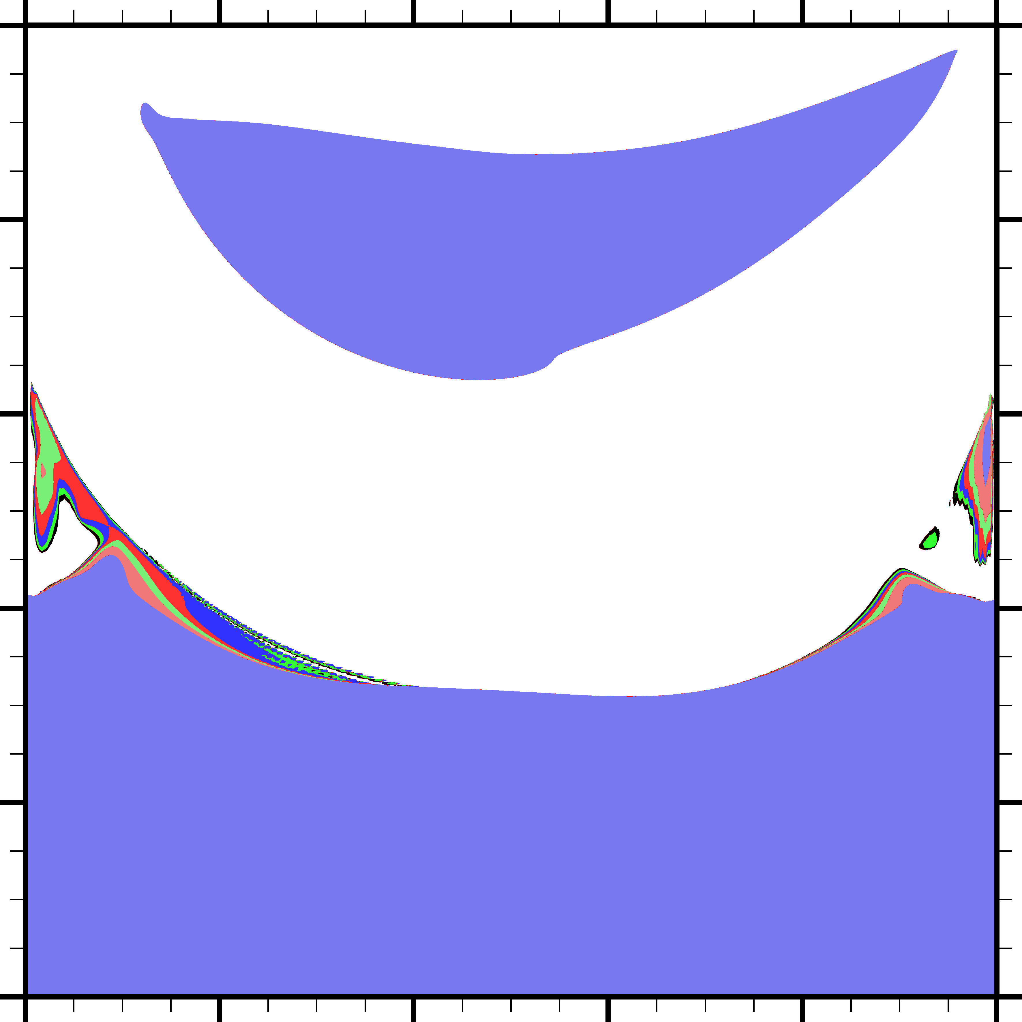
(a) Unyielded areas

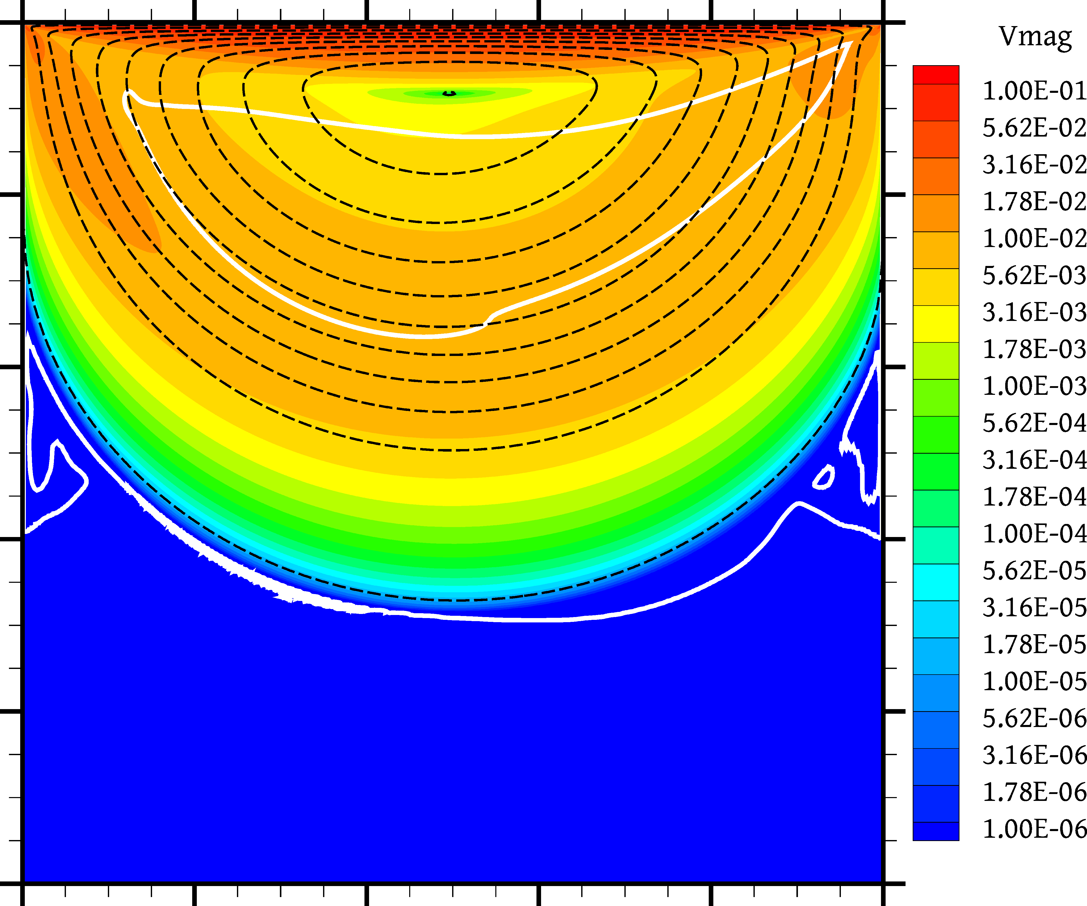
(b) $\|\underline{u}\|$ [$\mathrm{m}\mathrm{/}\mathrm{s}$]

Figure 11: 11(a) Yielded (white) and unyielded (colour) regions for the base case (Sec. 6.1). Different colours denote the extent of the unyielded regions at $t$ = 30, 60, 90, 120, 150, 180 and 210 $\mathrm{s}$ (the lower unyielded region is expanding with time). 11(b) Colour contours of the magnitude of the velocity vector at $t$ = 210 $\mathrm{s}$. The white lines are the yield lines ($\tau_{d}=\tau_{y}$) and the dashed black lines are streamlines, both at $t$ = 210 $\mathrm{s}$. The streamlines are plotted at equal streamfunction intervals.

A striking feature of the flow evolution is the slowness with which the stationary unyielded zone tends to obtain its final shape. Figure 11(a) shows that although the plug zone has reached its steady state already from $t$ = 30 $\mathrm{s}$, the stationary zone continues to expand even at $t$ = 210 $\mathrm{s}$. The shape of the yield line delimiting this zone is quite irregular. Furthermore, Fig. 11(b) shows that this zone is surrounded by an amount of fluid that is practically stationary and yet yielded. It is likely that this fluid will eventually become part of the stationary unyielded zone as $t\rightarrow\infty$, i.e. that the yield line will eventually lie somewhere close to the nearby streamline drawn in Fig. 11(b), which separates the fluid with near-zero velocity from that whose velocity is larger. However, to ascertain this the simulation would have to be prolonged to prohibitively long times; already the expansion of the lower unyielded zone from $t$ = 180 $\mathrm{s}$ to $t$ = 210 $\mathrm{s}$, marked in black colour in Fig. 11(a), is very small.

A related feature is that the magnitude of the deviatoric stress tensor, $\tau_{d}$, is very close to the yield stress throughout the aforementioned near-zero velocity region into which the lower unyielded zone is expanding. Thus, this region appears as an almost completely flat surface in the three-dimensional plot of $\tau_{d}$ in Fig. 12 (the surface outlined in dashed line contains fluid where $\tau_{d}$ is within $\pm 1$ $\mathrm{P}\mathrm{a}$ of $\tau_{y}$). Due to its distinctive features, we will refer to this region as a “transition zone”. In it, the fluid practically behaves as unyielded, although some of it can be formally yielded. The plug zone possesses no transition zone.

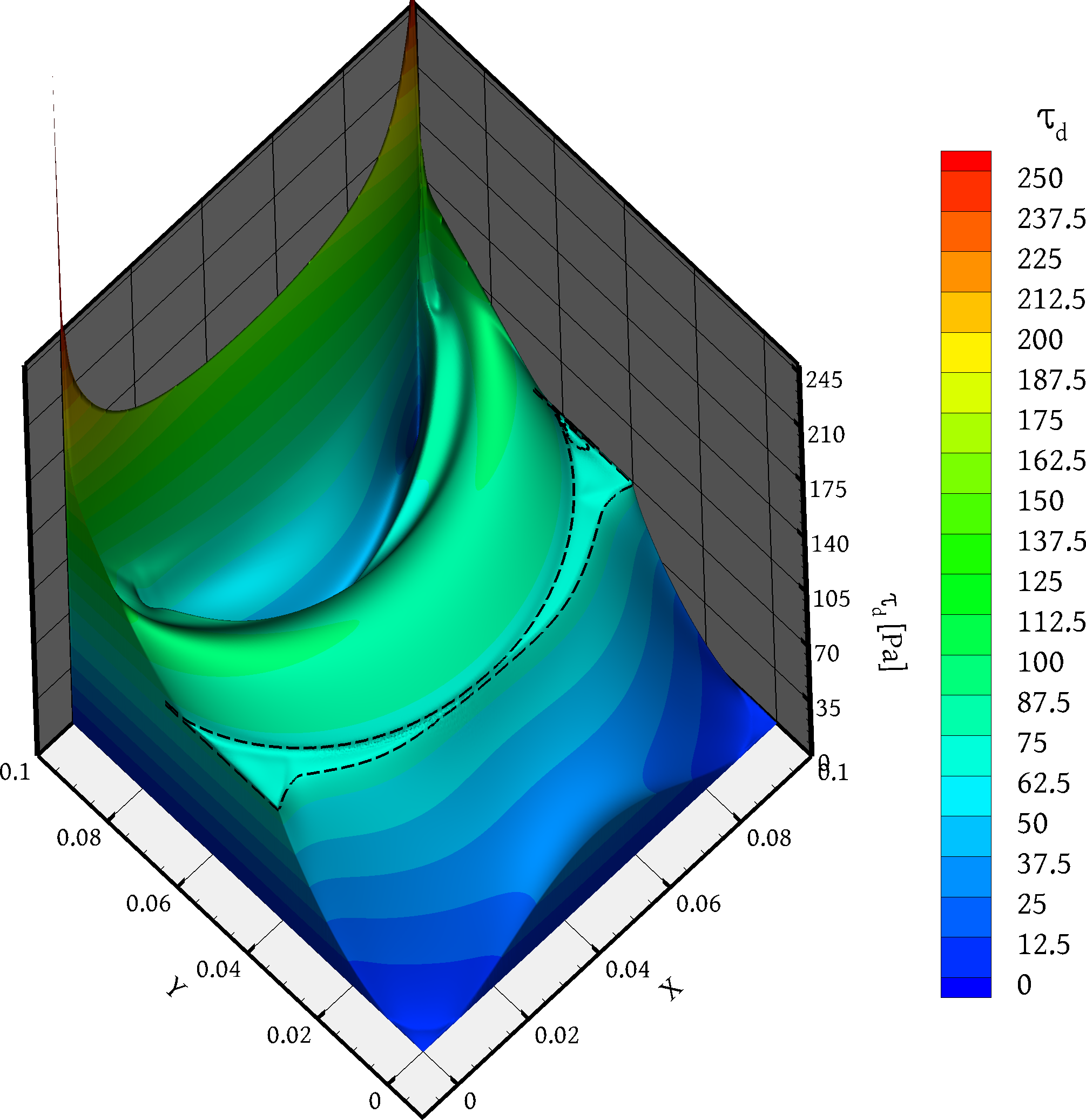
Figure 12: 3D contour plot of the base case results (Sec. 6.1) at $t$ = 210 $\mathrm{s}$. Both the colour contours and the plot height ($z$ axis) represent $\tau_{d}$. In addition, the dashed line encloses an area where $\tau_{d}\in[69,71]$ $\mathrm{P}\mathrm{a}$.

In order to explain the transition zone behaviour, we consider the constitutive equation (7) – (8) in the case that the fluid velocity is zero and $\tau_{d}$ is slightly above $\tau_{y}$. It becomes:

$$\frac{\partial\underline{\underline{\tau}}}{\partial t}\;=\;-\frac{G}{k^{\frac{1}{n}}}(\tau_{d}-\tau_{y})^{\frac{1}{n}}\frac{1}{\tau_{d}}\;\underline{\underline{\tau}}\;\equiv\;-r(\tau_{d})\;\underline{\underline{\tau}}$$ (71)

Since the function $r(\tau_{d})$ assumes only positive values, the minus sign on the right-hand side of Eq. (71) drives the components of $\underline{\underline{\tau}}$ towards zero as time passes, with a rate proportional to $r(\tau_{d})$ (and to the magnitude of those components themselves). Hence $\tau_{d}$ decreases towards zero as well (Eq. (9)). However, the rate at which they decrease, $r(\tau_{d})$, diminishes as $\tau_{d}\rightarrow\tau_{y}$ and in fact $r(\tau_{y})=0$. Therefore, $\tau_{d}$ actually converges towards $\tau_{y}$ and not to zero. This is what we observe happening inside the transition zone.

It is useful to consider also a scalar version of Eq. (71) ($\tau_{d}\equiv\tau$ in this case):

$$\frac{\mathrm{d}\tau}{\mathrm{d}t}\;=\;-\frac{G}{k^{\frac{1}{n}}}(\tau-\tau_{y})^{\frac{1}{n}}$$ (72)

For $n=1$, the solution to the above equation is

$$\tau-\tau_{y}\;=\;(\tau_{0}-\tau_{y})\,e^{-t/\lambda^{\prime}}$$ (73)

where $\tau_{0}$ is the value of $\tau$ at $t=0$ and $\lambda^{\prime}\equiv k/G$ is a relaxation time. This behaviour is similar to that of a Maxwell viscoelastic fluid, only that now $\tau$ decays exponentially towards $\tau_{y}$ instead of towards zero. For $n\neq 1$, Eq. (72) can be written as ($\lambda^{\prime}\equiv k^{1/n}/G$ now has units of $\mathrm{s}\mathrm{/}\mathrm{P}\mathrm{a}^{1-1/n}$):

$$\frac{\mathrm{d}(\tau-\tau_{y})}{\mathrm{d}t}\;=\;-\underbrace{\frac{1}{\lambda^{\prime}}(\tau-\tau_{y})}_{\mathclap{\text{rate of decay for }n=1}}(\tau-\tau_{y})^{\frac{1-n}{n}}$$ (74)

so that the rate of decay of $\tau$ towards $\tau_{y}$ equals that for $n=1$ multiplied by a factor of $(\tau-\tau_{y})^{(1-n)/n}$. If $n<1$, as is the present choice but also the most common case, then $(1-n)/n>0$ and as time progresses and $\tau\rightarrow\tau_{y}$, the extra factor $(\tau-\tau_{y})^{(1-n)/n}$ tends to zero, and the rate of decay becomes progressively smaller than that of the $n=1$ case, eventually becoming infinitesimal compared to it. This behaviour is explained physically by the fact that the relaxation time (Eq. (21)) is proportional to the fluid viscosity, which resists recovery from deformation (relaxation), and inversely proportional to the elastic modulus, which drives towards such recovery. For shear-thinning fluids ($n<1$), the viscosity increases as $\tau$ becomes smaller and, in the SHB and HB models, tends to infinity as $\tau\rightarrow\tau_{y}$. Thus, for these fluids the relaxation time tends to infinity as $\tau\rightarrow\tau_{y}$. The opposite happens in the less common case of $n>1$.

By dividing both sides of Eq. (14) by $\operatorname{\mathit{Re}}$, because $Re$ is very small (Table 3), it becomes apparent that the fluid particle accelerations (the left-hand side of that equation) are large and the velocity adjusts very quickly to force changes (the inertial time scales are very small). Thus, the velocity should vary at the same rate as these forces, i.e. the velocity and stress variations should go hand-in-hand (the boundary conditions are not a source of variation as the lid velocity remains constant for $t>T$ = 1 $\mathrm{s}$). However, in Fig. 10 the velocity field appears to reach a steady state much faster than the stress field. This can be explained by observing that the stress actually also evolves quickly over most of the domain, the relaxation time $\lambda$ = 0.255 $\mathrm{s}$ (Table 3) being quite small compared to the time scale of stress evolution in Fig. 10(b), except in the transition zone where the definition (21) is not representative and the actual relaxation time tends to infinity as time passes. There, the stress magnitude is of the order of $\tau_{y}$, so its local slow evolution has a noticeable impact on the average stress trace plotted in Fig. 10. The velocity does follow the stress evolution, but since it is almost zero in this zone its local variations caused by the local stress evolution have a negligible impact on the overall kinetic energy plotted in Fig. 10. We noticed that between $t$ = 30 $\mathrm{s}$ and $t$ = 210 $\mathrm{s}$ the change in the velocity components at any point in the domain is of the order of $10^{-6}$ $\mathrm{m}\mathrm{/}\mathrm{s}$, except in the transition zone where it can be about five times larger.

Figure 13 shows vertical profiles of most flow variables along the centreline ($x=L/2$, Figs. 13(a) and 13(b)) and close to the right wall ($x=0.95L$, Figs. 13(c) and 13(d)). Two profiles are drawn for each variable, one at time $t$ = 30 $\mathrm{s}$ and one at $t$ = 210 $\mathrm{s}$. These profiles are identical inside the yielded and plug zones, and only deviate very slightly inside the bottom unyielded zone. Thus the steady state has largely been reached already at $t$ = 30 $\mathrm{s}$. The vertical line at $x=0.95L$ cuts through a significant width of the transition zone, which can be recognised by the vertical line segment where $\tau_{d}\approx\tau_{y}$ in Fig. 13(c) (approximately from $y$ = 0.041 $\mathrm{m}$ to $y$ = 0.051 $\mathrm{m}$). A close-up view of the variation of $\tau_{d}$ in the transition zone is shown in the inset of the same figure, where one can see that as time passes, $\tau_{d}$ decreases towards $\tau_{y}$ throughout the zone.

Interestingly, Fig. 13(a) shows that the normal stress component $\tau_{11}$ tends to vary discontinuously across the boundary of the lower unyielded zone as time passes. The possibility of the SHB model producing solutions with discontinuous stress components and/or velocity gradients was noted and discussed in [39, 22], where it was attributed to the combination of the upper convective derivative and the viscoplastic “max” term. Nevertheless, as noted in [39], stress discontinuities must be such that the components of the force $\nabla\cdot\underline{\underline{\sigma}}=\nabla\cdot(\underline{\underline{\tau}}-p\underline{\underline{I}})$ remain bounded (discontinuities in $\underline{\underline{\tau}}$ that lead to infinite derivatives in $\nabla\cdot\underline{\underline{\tau}}$ can exist if they are counterbalanced by opposite discontinuities in $-p\underline{\underline{I}}$). Otherwise, at a point of discontinuity there will result a finite (i.e. non-zero) force acting on an infinitesimal mass, producing infinite acceleration and making the velocity field discontinuous, but this violates the continuity equation for an incompressible medium. In our case though, the variation of $\tau_{11}$ in the $x_{2}$ direction does not cause any force on the fluid (there is no $\partial\tau_{11}/\partial x_{2}$ derivative in $\nabla\cdot\underline{\underline{\tau}}$) and is therefore allowed to be discontinuous.

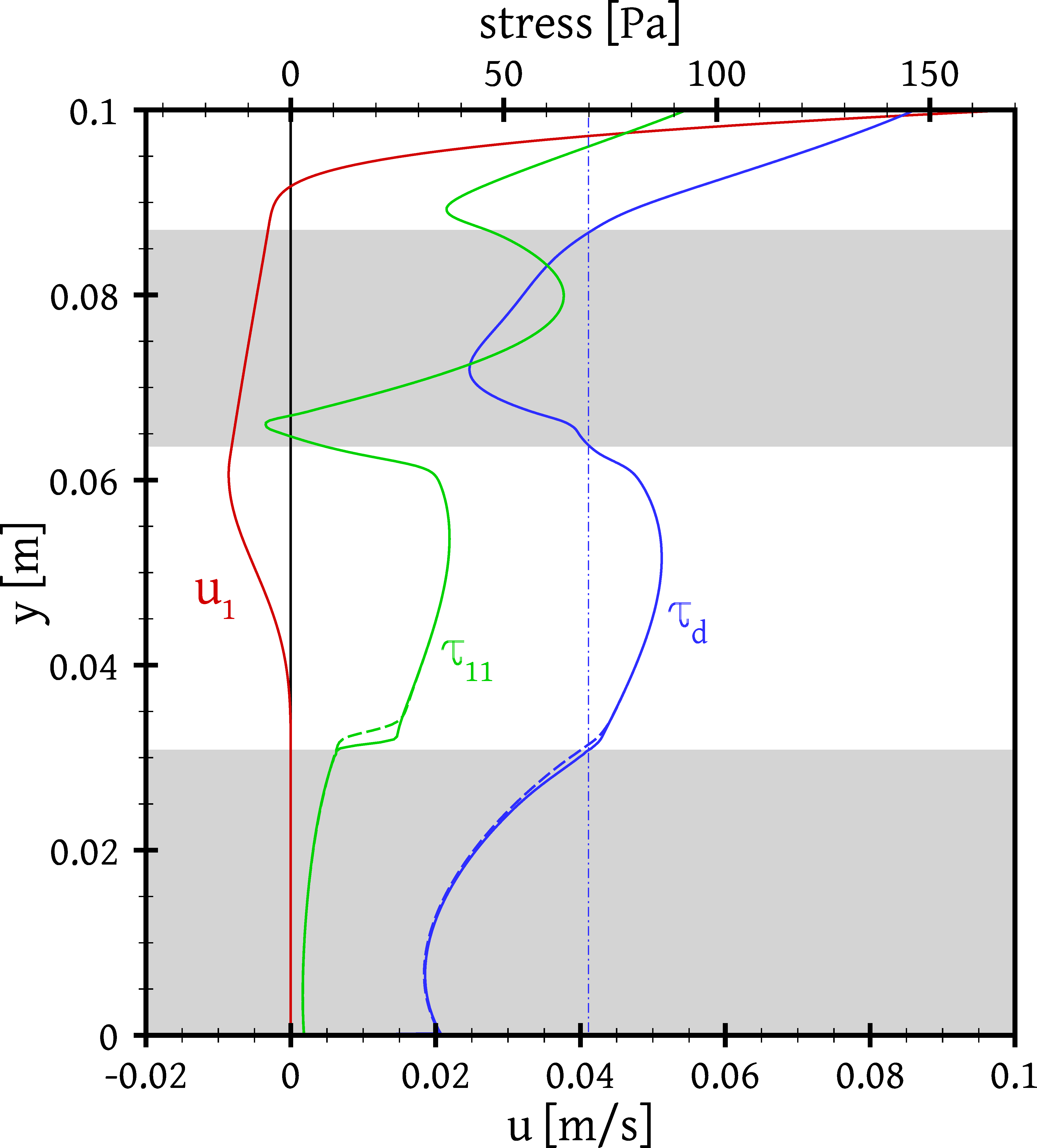
(a) $u_{1}$, $\tau_{11}$ and $\tau_{d}$ at $x=L/2$.

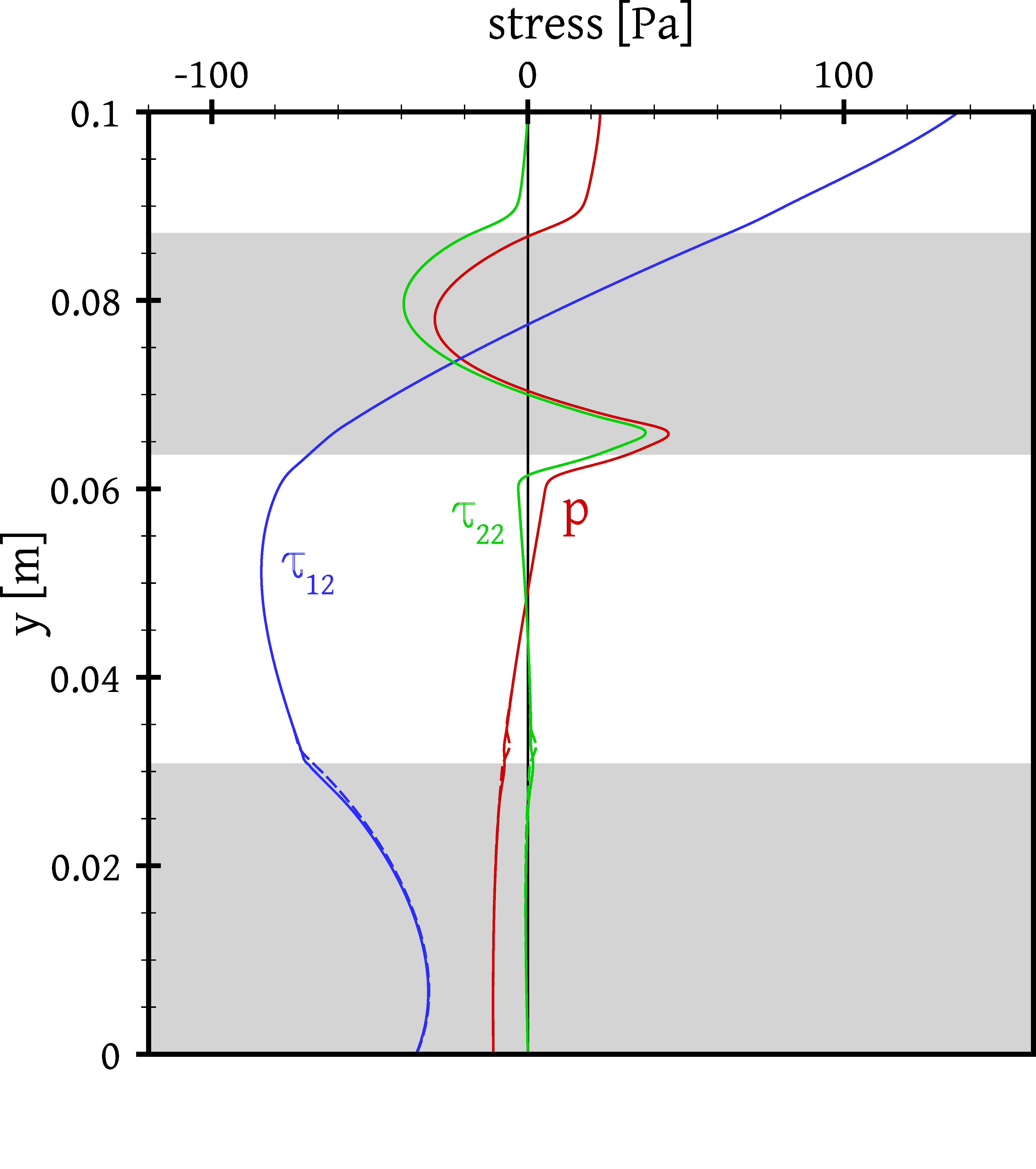
(b) $p$, $\tau_{22}$ and $\tau_{12}$ at $x=L/2$.

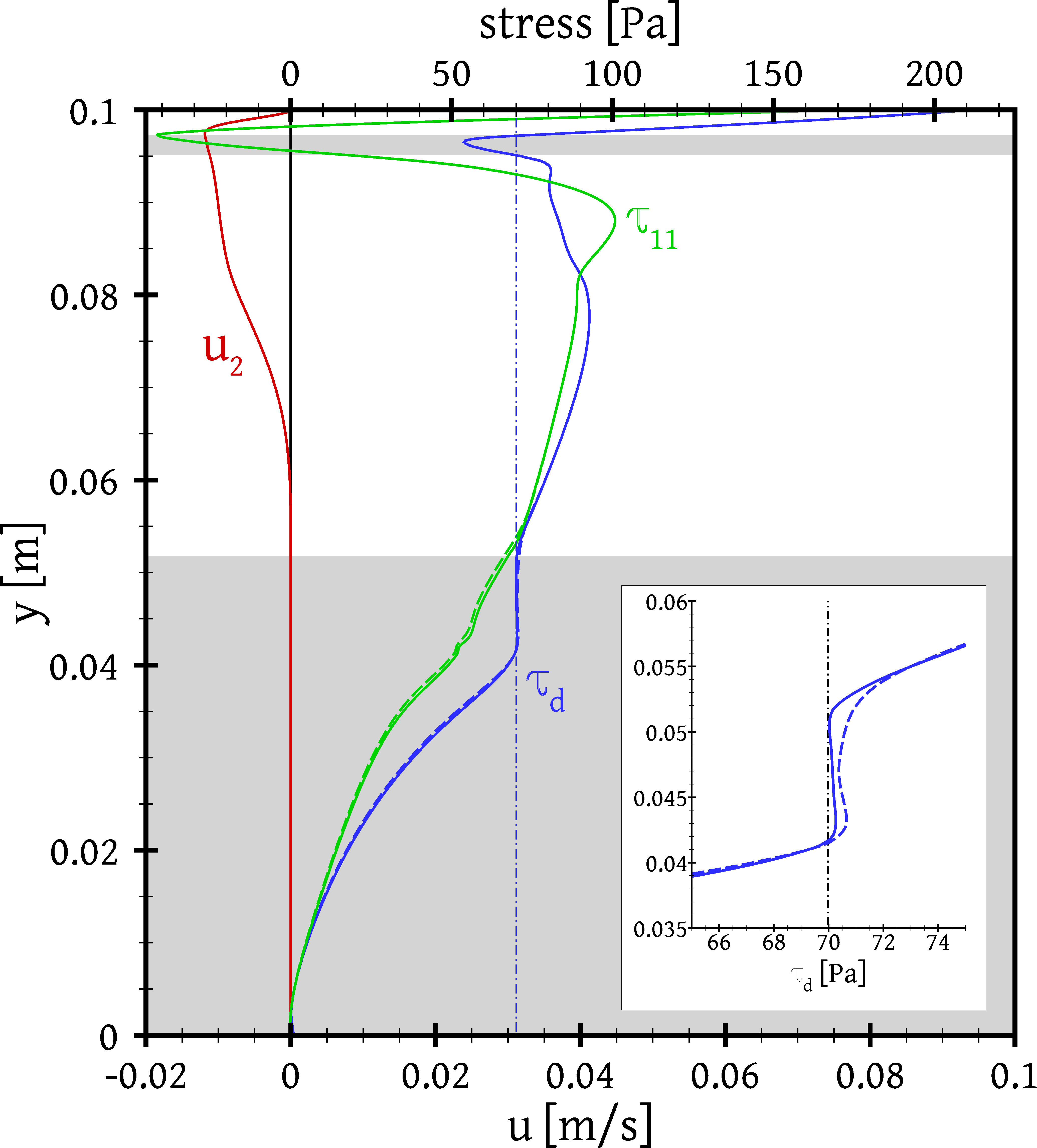
(c) $u_{2}$, $\tau_{11}$ and $\tau_{d}$ at $x=0.95L$.

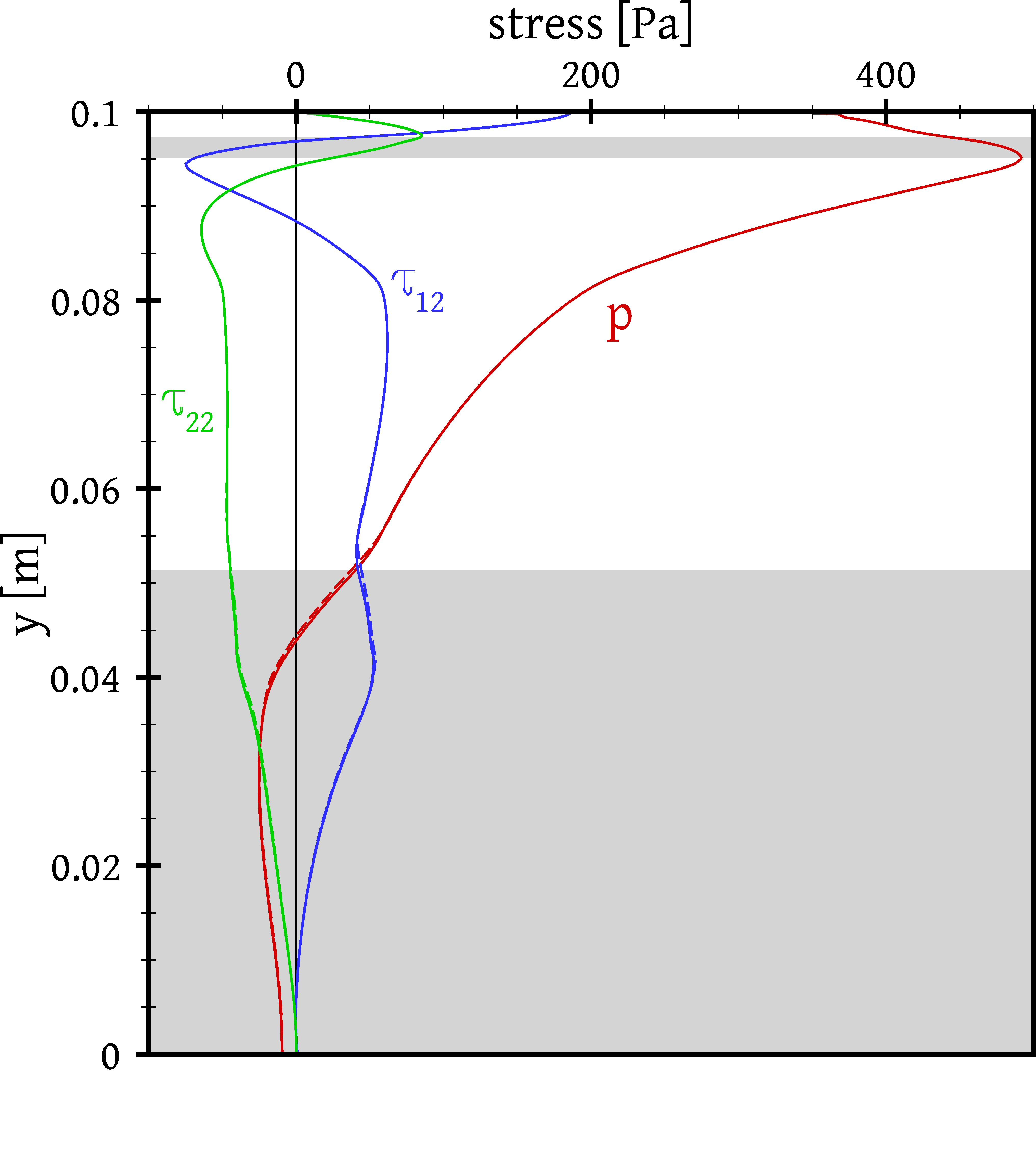
(d) $p$, $\tau_{22}$ and $\tau_{12}$ at $x=0.95L$.

Figure 13: Profiles of some dependent variables along vertical lines, for the base case (Sec. 6.1): 13(a), 13(b) at the vertical centreline ($x=0.5L$); 13(c), 13(d) close to the right wall ($x=0.95L$). Dashed / continuous lines denote profiles at $t$ = 30 $\mathrm{s}$ / 210 $\mathrm{s}$, respectively. The vertical dash-dot lines in 13(a) and 13(c) mark the yield stress value $\tau_{y}$. The unyielded and transition regions are shaded. The inset in 13(c) shows a close-up view of the $\tau_{d}$ profile at $y\in[0.035,0.060]$ $\mathrm{m}$.

6.2 Varying the lid velocity

Next we examine the flow driven by higher ($U$ = 0.4 $\mathrm{m}\mathrm{/}\mathrm{s}$) and lower ($U$ = 0.025 $\mathrm{m}\mathrm{/}\mathrm{s}$) lid velocities, which affects the dimensionless numbers as shown in Table 3. Lowering the velocity increases the Bingham number and decreases the Weissenberg number, i.e. it accentuates the plastic character of the flow at the expense of its elastic character. The $\operatorname{\mathit{Re}}$ values listed in Table 3 suggest that inertia effects should be negligible for $U$ = 0.025 and 0.100 $\mathrm{m}\mathrm{/}\mathrm{s}$, but should be slightly noticeable for $U$ = 0.400 $\mathrm{m}\mathrm{/}\mathrm{s}$. The Table shows also that $\lambda$ increases as $U$ decreases; at lower velocities the apparent viscosity $\eta$, Eq. (21), is higher and therefore the stresses relax more slowly. Thus, we expect the flow to evolve more slowly as $U$ is reduced.

The lid velocity is again increased gradually according to Eq. (68) with $T=L/U$. Figure 10(a) shows that the KE of the fluid builds up in an oscillatory manner, usually with an overshoot, due to elastic effects. The larger $U$ is, the more prominent and persistent the oscillations. Figure 10(b) confirms that the stress evolution is slower at lower $U$, as discussed above. The top row of Fig. 14 shows the corresponding near-steady-state flow fields. Increasing the lid velocity leads to less unyielded material in the cavity, and the vortex has more free space to move away from the lid (see the $y_{c}$ coordinate in Table 4). In each case there is a transition zone between the bottom unyielded zone and the yielded material, with the former not having yet expanded throughout the near-zero velocity region. The number and density of streamlines in Fig. 14 shows that at higher $\operatorname{\mathit{Bn}}$ the flow is weaker and more confined to a thin layer below the lid while circulation is very weak in the rest of the domain. This is reflected also in the normalised KE diagram 10(a), and also in the normalised vortex strengths listed in Table 4. That Table also shows that the vortex lies slightly to the left of the centreline, as is typical of viscoelastic lid-driven cavity flows, although this shift is not as pronounced as for the Oldroyd-B flows of Table 1. Interestingly, as $U$ is increased the vortex centre moves towards the centreline despite $\operatorname{\mathit{Wi}}$ increasing; this could be due to inertia effects that will be discussed in Sec. 6.3.

Table 4: Dimensionless coordinates of the centre of the vortex $(\tilde{x}_{c},\tilde{y}_{c})\equiv(x_{c}/L,y_{c}/L)$ and value of the streamfunction there $\tilde{\psi}_{c}\equiv\psi_{c}/(LU)$, for various cases, at steady-state.

	SHB			HB
	$\tilde{x}_{c}$	$\tilde{y}_{c}$	$\tilde{\psi}_{c}$	$\tilde{x}_{c}$	$\tilde{y}_{c}$	$\tilde{\psi}_{c}$
$U$ = 0.025 $\mathrm{m}\mathrm{/}\mathrm{s}$	$0.495$	$0.935$	$-0.0211$	$0.500$	$0.933$	$-0.0214$
$U$ = 0.100 $\mathrm{m}\mathrm{/}\mathrm{s}$	$0.495$	$0.917$	$-0.0270$	$0.500$	$0.915$	$-0.0281$
$U$ = 0.400 $\mathrm{m}\mathrm{/}\mathrm{s}$	$0.500$	$0.899$	$-0.0333$	$0.505$	$0.897$	$-0.0352$
$U$ = 0.100 $\mathrm{m}\mathrm{/}\mathrm{s}$, slip	$0.482$	$0.846$	$-0.0125$	$0.500$	$0.853$	$-0.0112$

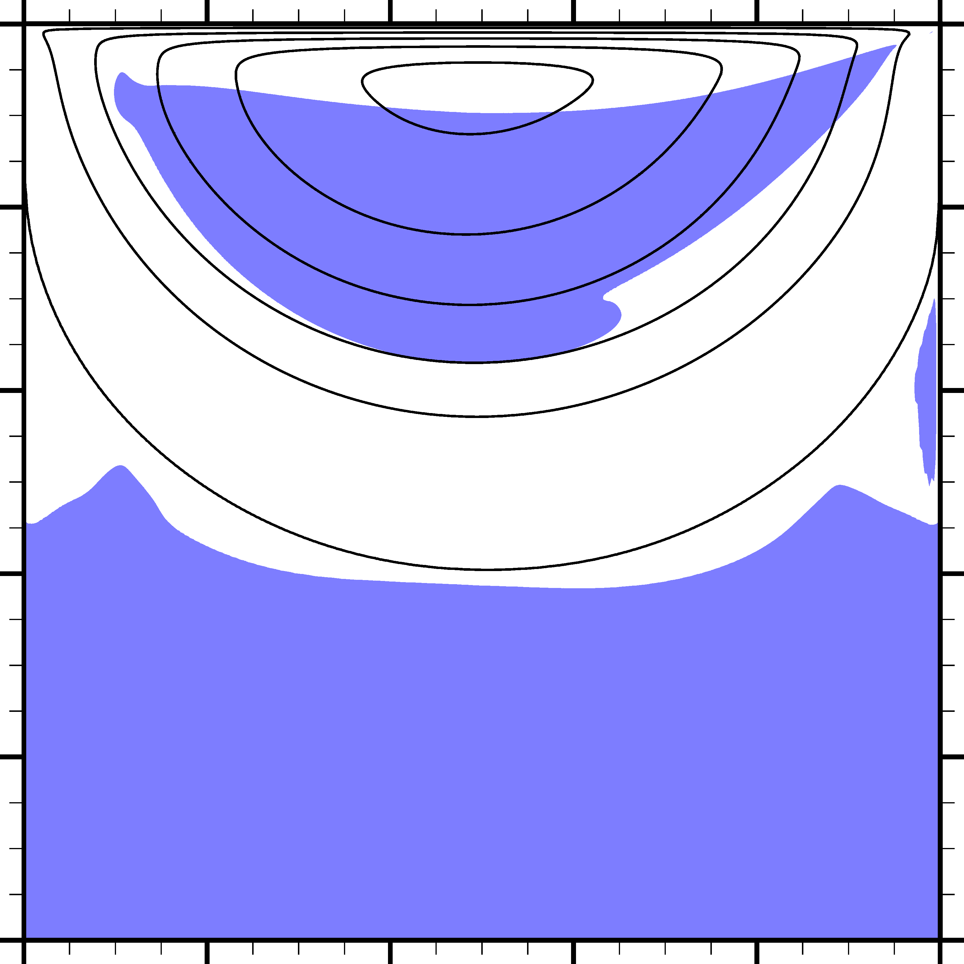
(a) SHB, $U=0.025$ $\mathrm{m}\mathrm{/}\mathrm{s}$, $t$ = 90 $\mathrm{s}$

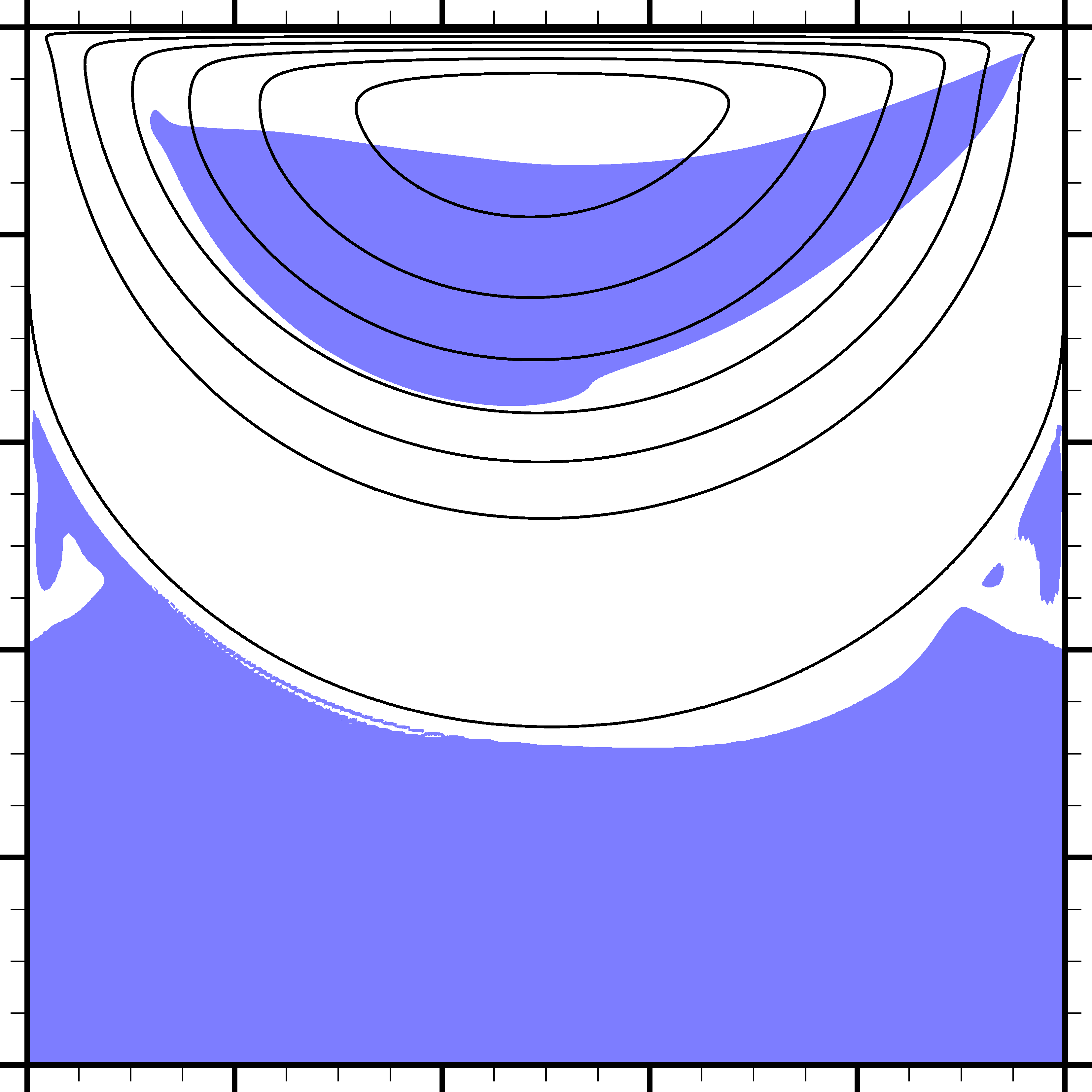
(b) SHB, $U=0.100$ $\mathrm{m}\mathrm{/}\mathrm{s}$, $t$ = 210 $\mathrm{s}$

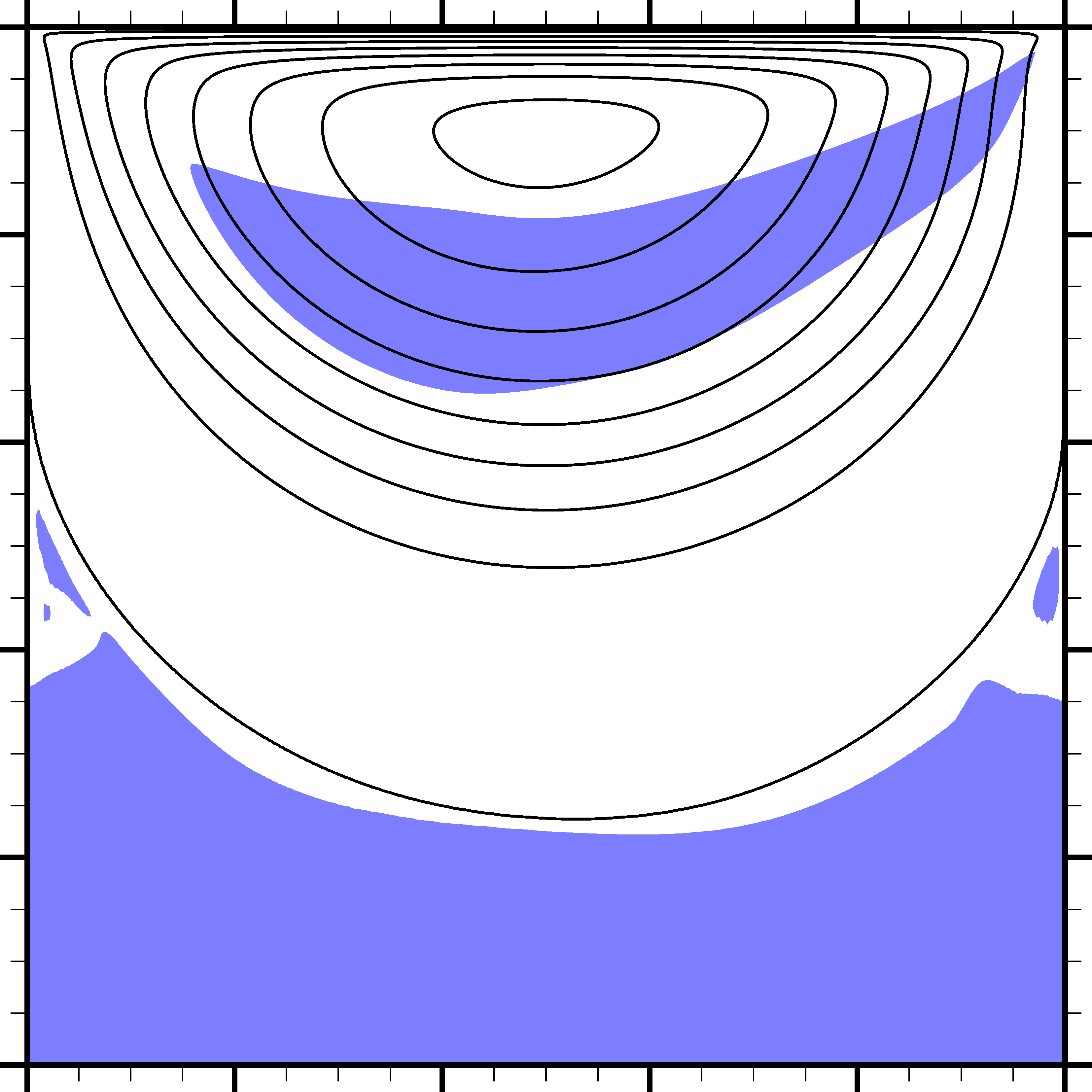
(c) SHB, $U=0.400$ $\mathrm{m}\mathrm{/}\mathrm{s}$, $t$ = 60 $\mathrm{s}$

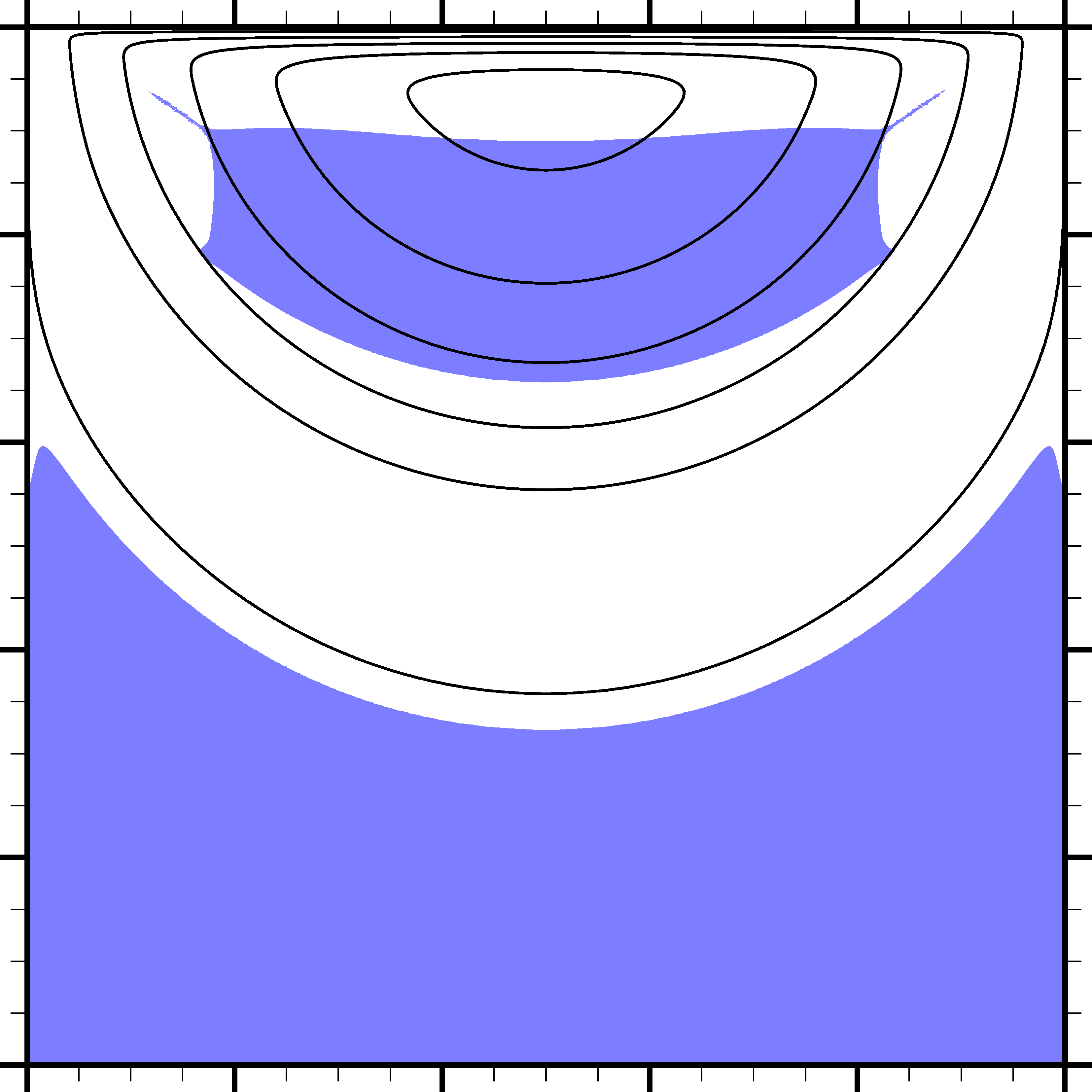
(d) HB, $U=0.025$ $\mathrm{m}\mathrm{/}\mathrm{s}$

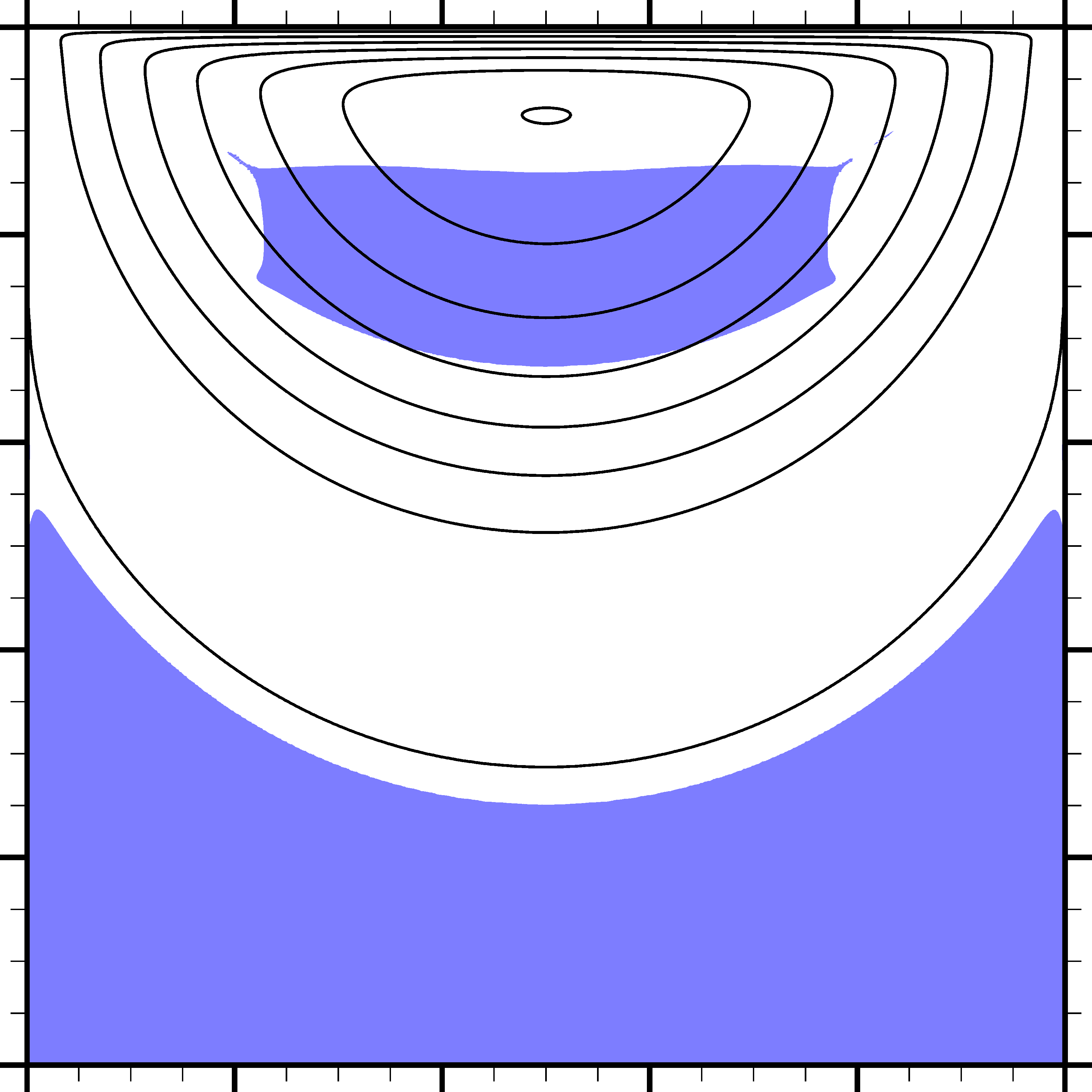
(e) HB, $U=0.100$ $\mathrm{m}\mathrm{/}\mathrm{s}$

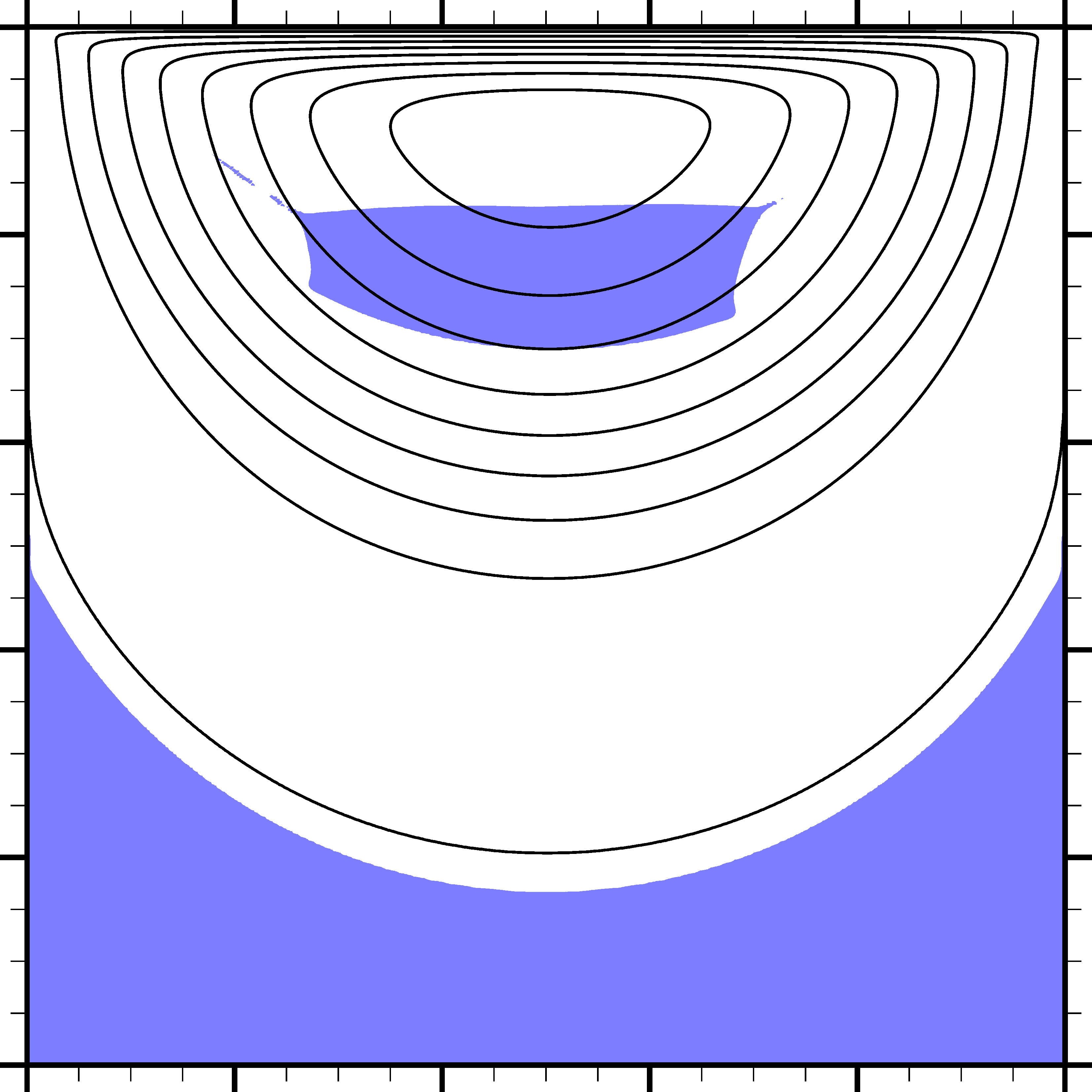
(f) HB, $U=0.400$ $\mathrm{m}\mathrm{/}\mathrm{s}$

Figure 14: Top row: SHB flow snapshots at the times indicated, for different lid velocities. Bottom row: corresponding HB steady-state flowfields. The unyielded regions are shown shaded; the lines are instantaneous streamlines, plotted at streamfunction values $\psi/(UL)$ = 0.04, 0.08, 0.12 etc., plus a $\psi$ = $5\text{\times}{10}^{-6}$ $\mathrm{m}^{3}\mathrm{/}\mathrm{s}$ streamline just above the lower unyielded region.

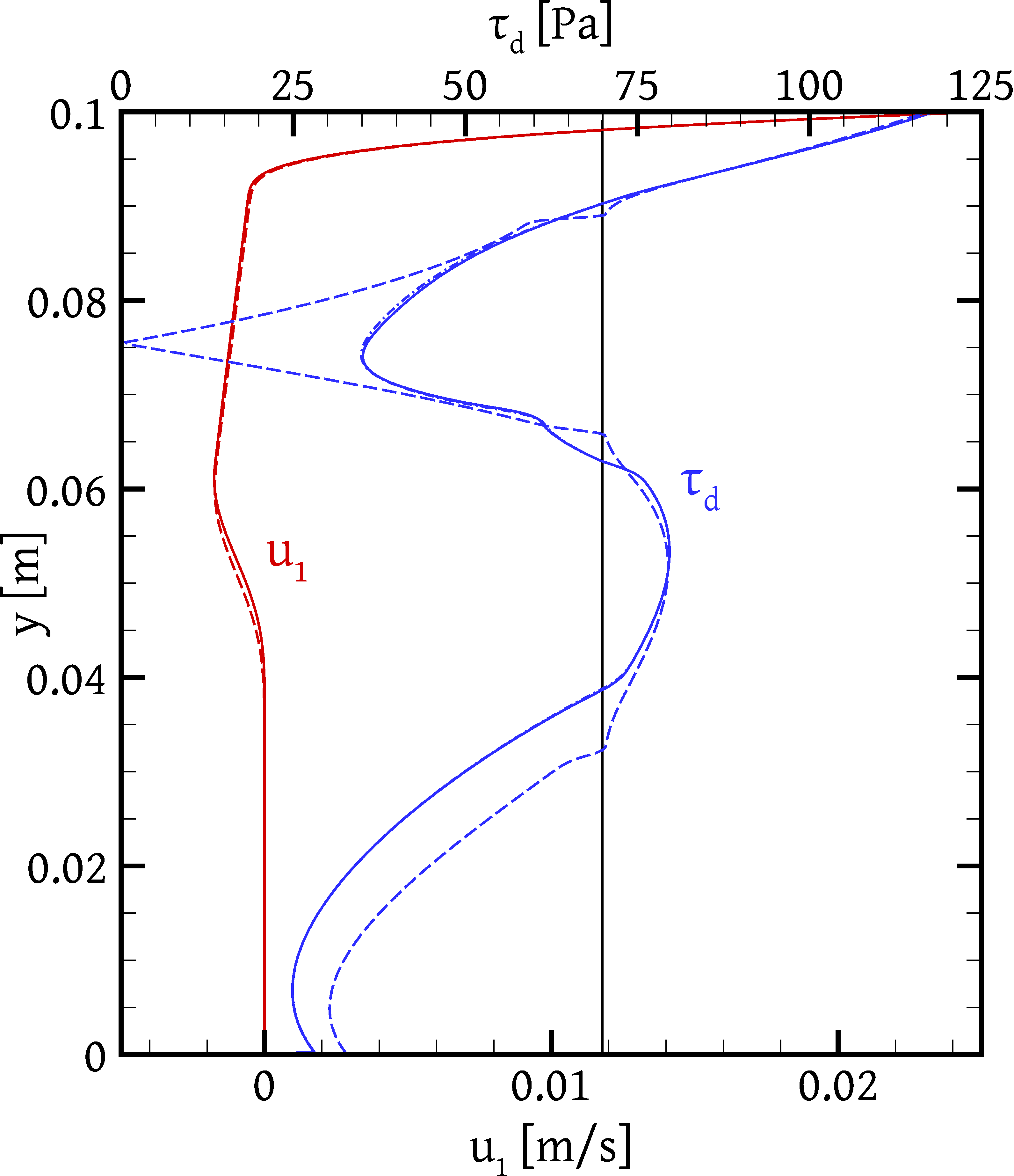
(a) $U=0.025$ $\mathrm{m}\mathrm{/}\mathrm{s}$

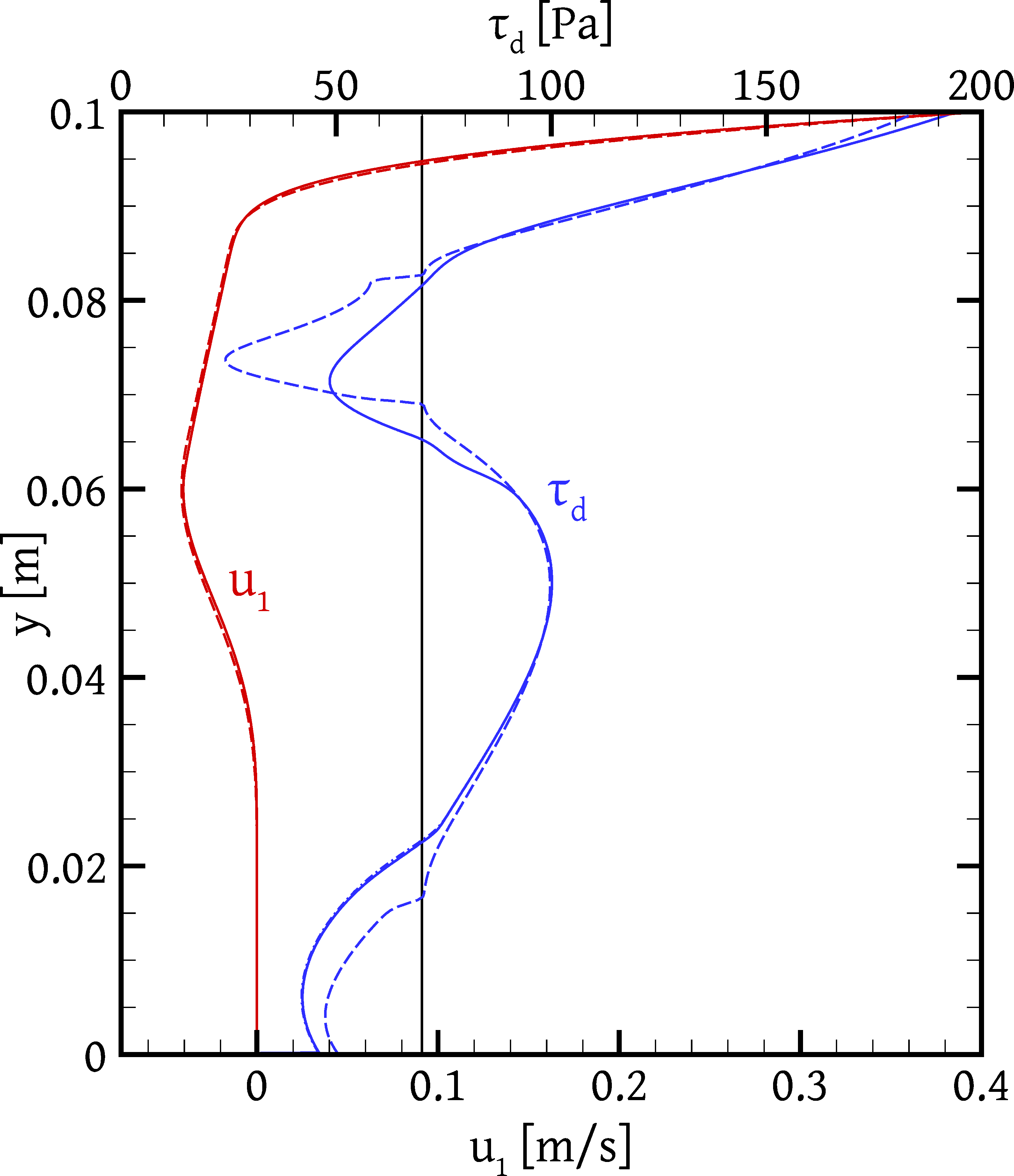
(b) $U=0.400$ $\mathrm{m}\mathrm{/}\mathrm{s}$

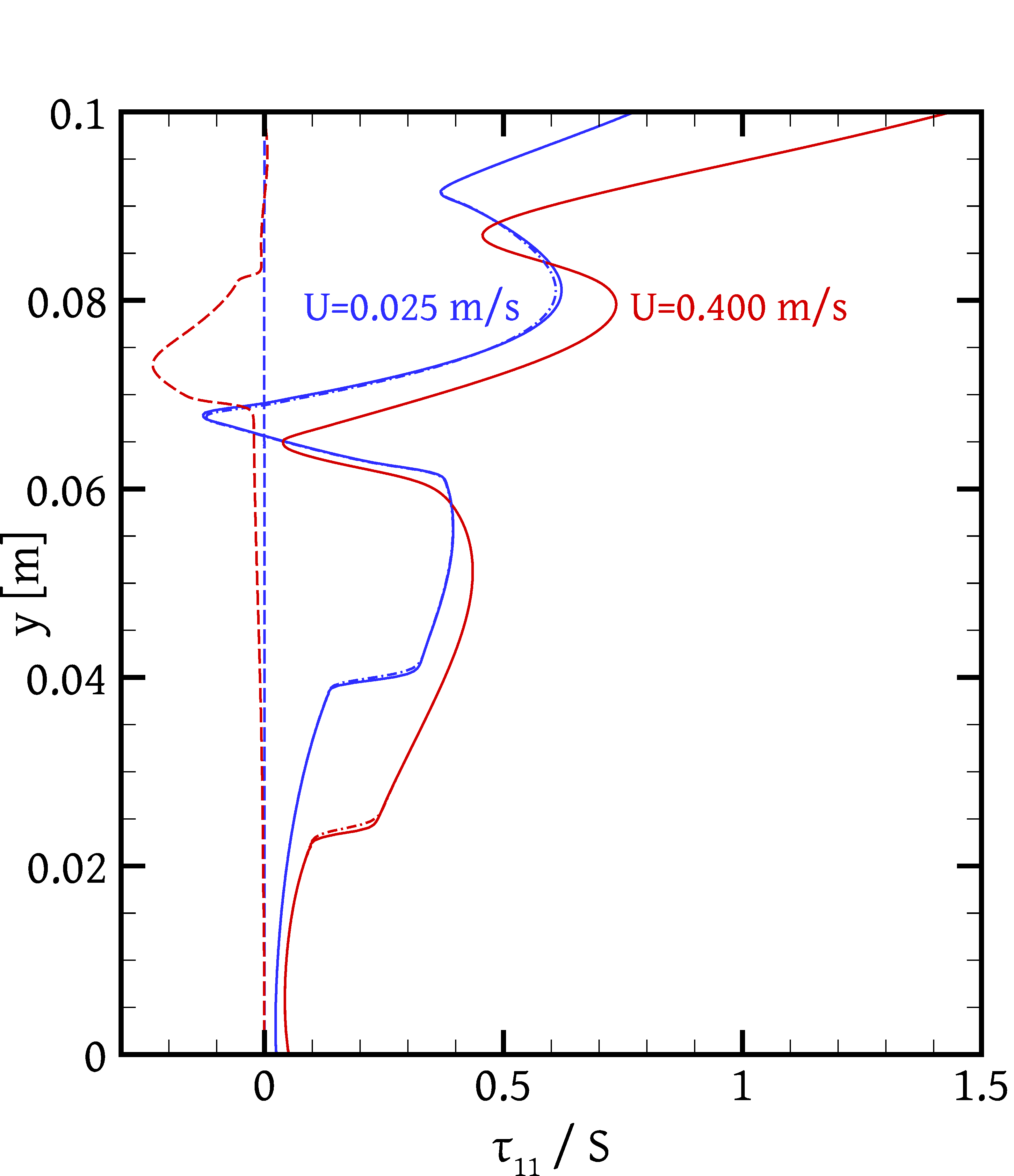
(c) $\tau_{11}/S$

Figure 15: Profiles of $u_{1}$ and $\tau_{d}$ for $U$ = 0.025 $\mathrm{m}\mathrm{/}\mathrm{s}$ 15(a) and $U$ = 0.400 $\mathrm{m}\mathrm{/}\mathrm{s}$ 15(b), and profiles of $\tau_{11}/S$ for both $U$’s 15(c). All profiles are along the vertical centreline ($x=L/2$). Continuous lines: SHB profiles at $t$ = 90 $\mathrm{s}$ ($U$ = 0.025 $\mathrm{m}\mathrm{/}\mathrm{s}$) and $t$ = 60 $\mathrm{s}$ ($U$ = 0.400 $\mathrm{m}\mathrm{/}\mathrm{s}$); dash-dot lines: SHB profiles at 30 $\mathrm{s}$ earlier; dashed lines: HB steady-state profiles. In 15(a) and 15(b) the vertical lines mark the yield stress.

6.3 Comparison with the classic HB model

Since the HB equation is used extensively to model viscoplastic flows, we compare its predictions against those of the SHB equation in order to get a feel of the error involved in neglecting elastic effects. The HB simulations were carried out by performing Papanastasiou regularisation [75], implemented as [76]:

$$\underline{\underline{\tau}}\;=\;\eta\dot{\underline{\underline{\gamma}}}\;,\qquad\eta\;=\;\frac{\tau}{\dot{\gamma}}\;\approx\;\frac{(\tau_{y}+k\dot{\gamma}^{n})(1-e^{-\dot{\gamma}/\epsilon})}{\dot{\gamma}}$$ (75)

where the regularisation parameter $\epsilon$ determines the accuracy of the approximation. This method was used for simulating lid-driven cavity Bingham flows in [24, 34], where it was noticed that the equations became too stiff to solve for $\epsilon<1/400$. However, with the present method, and using a continuation procedure where $\epsilon$ is progressively halved, solutions for $\epsilon$ = 1/128,000 were obtained. We performed steady-state simulations (since the steady-state of classic viscoplastic flows does not depend on the initial conditions) where the HB parameters $\tau_{y}$, $k$ and $n$ have the same values as for the SHB fluid (Table 2).

The flowfields, depicted in the second row of Fig. 14, are much more symmetric than their SHB counterparts. In HB lid-driven cavity flow, the only source of asymmetry is inertia. Inertial effects are imperceptible for $U$ = 0.025 and 0.100 $\mathrm{m}\mathrm{/}\mathrm{s}$ (Figs. 14(d) and 14(e)) and only slightly noticeable for $U$ = 0.400 $\mathrm{m}\mathrm{/}\mathrm{s}$ (Fig. 14(d)), which is in accord with the corresponding $\operatorname{\mathit{Re}}$ values listed in Table 3. So, for $U$ = 0.4 $\mathrm{m}\mathrm{/}\mathrm{s}$ the vortex centre is shifted slightly towards the right (Table 4), whereas at the lower $U$’s it is almost exactly on the centreline. Also, in Fig. 14(f) one can see that the upper unyielded (plug) region is somewhat stretched towards the left. These features are opposite to those of the SHB case, where elasticity causes the vortex centre to move towards the left and the plug region to stretch towards the right. The opposite effects of inertia and elasticity have been noted also in [36, 77, 29].

Figure 14 and Table 4 show that the union of the lower unyielded and transition zones in SHB flow is slightly larger than the corresponding HB stationary regions, pushing the SHB vortex upwards and lowering its strength compared to the HB case. Figures 15(a) and 15(b) show that the SHB and HB velocity profiles along the vertical centreline are very similar; the $\tau_{d}$ profiles are somewhat more dissimilar but still not far apart, especially in the yielded regions. In the unyielded regions they cannot be expected to be similar due to the stress indeterminacy of the HB model (the currently predicted HB stress field in the unyielded regions is one of infinite possibilities, the one conforming to the Papanastasiou regularisation). Profiles of $\tau_{11}$ are plotted in Fig. 15(c); for HB flow, due to the symmetric flowfield and $\tau_{11}$ being proportional to $\partial u_{1}/\partial x_{1}$, this stress component is nearly zero, except inside the plug region for $U$ = 0.400 $\mathrm{m}\mathrm{/}\mathrm{s}$, which is somewhat asymmetric (Fig. 14(f)). The SHB stresses, on the other hand, are significant due to elasticity, especially in the higher $U$ case which corresponds to higher $\operatorname{\mathit{Wi}}$. Finally, we note that in Fig. 15 two SHB profiles are plotted for each lid velocity: at $t$ = 60 and 90 $\mathrm{s}$ for $U$ = 0.025 $\mathrm{m}\mathrm{/}\mathrm{s}$, and at $t$ = 30 and 60 $\mathrm{s}$ for $U$ = 0.400 $\mathrm{m}\mathrm{/}\mathrm{s}$. These profiles are hardly distinguishable, indicating that the steady state for $U$ = 0.025 $\mathrm{m}\mathrm{/}\mathrm{s}$ has been practically reached at $t$ = 60 $\mathrm{s}$, and for $U$ = 0.400 $\mathrm{m}\mathrm{/}\mathrm{s}$ at $t$ = 30 $\mathrm{s}$.

Next, we performed a couple of simulations similar to the base case, only that we artificially increased the elastic modulus to 10 and 100 times the original value listed in Table 2. This reduces the relaxation times by factors of 10 and 100, respectively, so that the SHB material becomes more inelastic and its predictions should tend to match those of the HB model. Due to the smaller relaxation times, we also used smaller time steps: starting from an initial time step of $5\text{\times}{10}^{-5}$ $\mathrm{s}$ in both cases, we allowed the time step to increase up to $\Delta t_{\max}$ = $1.5\text{\times}{10}^{-3}$ $\mathrm{s}$ and ${10}^{-4}$ $\mathrm{s}$ in the $G$ = 4,000 $\mathrm{P}\mathrm{a}$ and $G$ = 40,000 $\mathrm{P}\mathrm{a}$ cases, respectively. The simulations were stopped at $t$ = 50 $\mathrm{s}$ and 10 $\mathrm{s}$ respectively, and in the $G$ = 40,000 $\mathrm{P}\mathrm{a}$ case the lid acceleration period (Eq. (68)) was reduced to 0.01 $\mathrm{s}$. Figure 16 shows that the SHB and HB streamlines converge rapidly with increasing $G$, while Fig. 17 shows that convergence is not as rapid for the stresses. Of course, for $\tau_{d}<\tau_{y}$ (top row of Fig. 17) we cannot expect the SHB and HB stresses to ever match, due to the aforementioned indeterminacy of the HB stress tensor in the unyielded regions. The yield lines (second row of Fig. 17) appear to converge, but at a slow pace. Despite the shorter duration of the $G$ = 40,000 $\mathrm{P}\mathrm{a}$ simulation, Fig. 17(f) shows that during this time the transition zone has evolved further than in the lower $G$ cases, due to the much shorter relaxation times. The same figure reveals some slight spurious stress oscillations on the lower yield line (can also be seen in Fig. 17(d)). They could be due to the near-zero velocities there, which complicates the application of upwinding within CUBISTA. Finally, the last row of Fig. 17 shows that within the yielded region the $\tau_{d}$ predictions of the two models are quite close, even for $G$ = 400 $\mathrm{P}\mathrm{a}$. A persistent discrepancy between the two models at the sides of the plug region seen in Fig. 17(i) may be due to spatial or temporal discretisation errors, regularisation, etc.

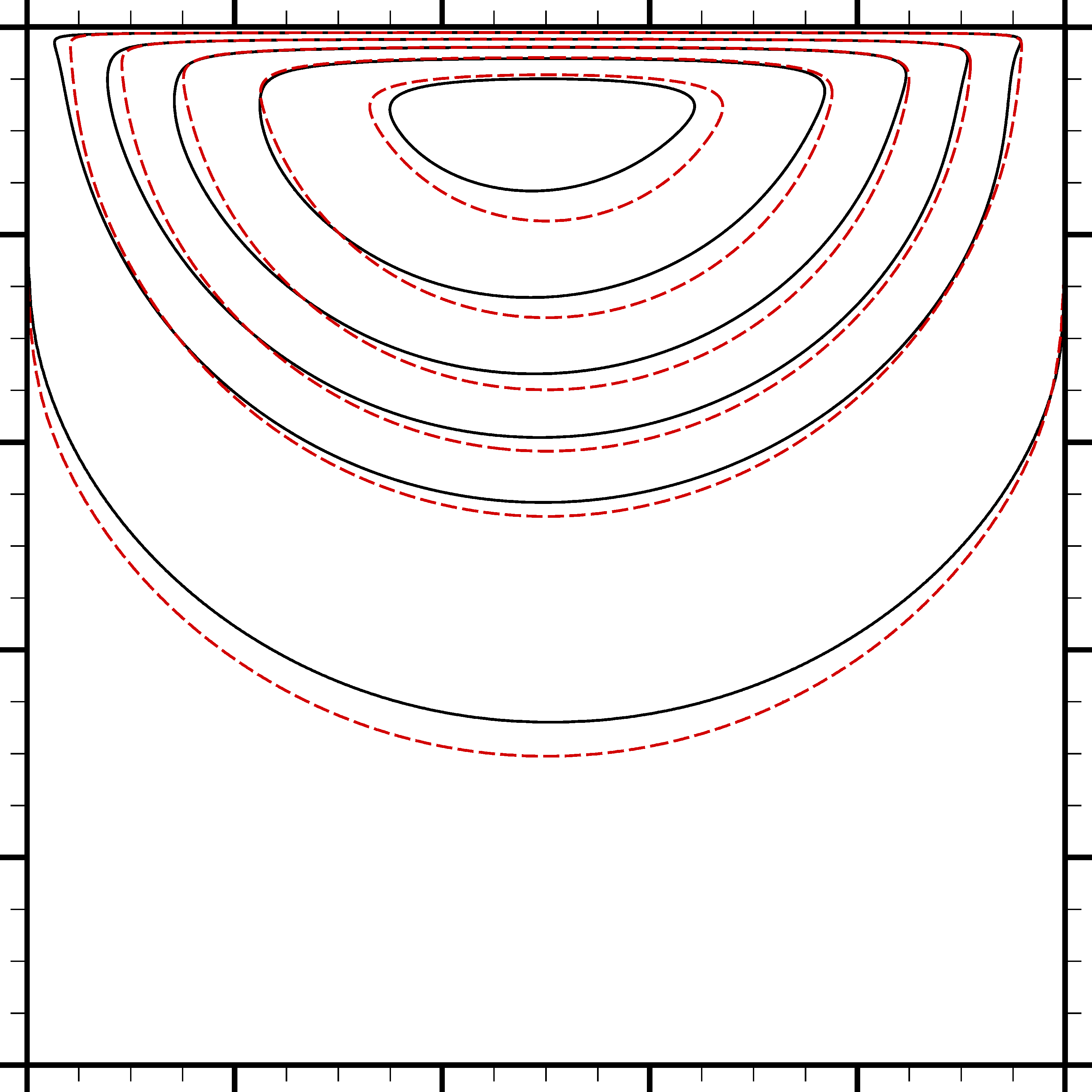
(a) $G=400$ $\mathrm{P}\mathrm{a}$

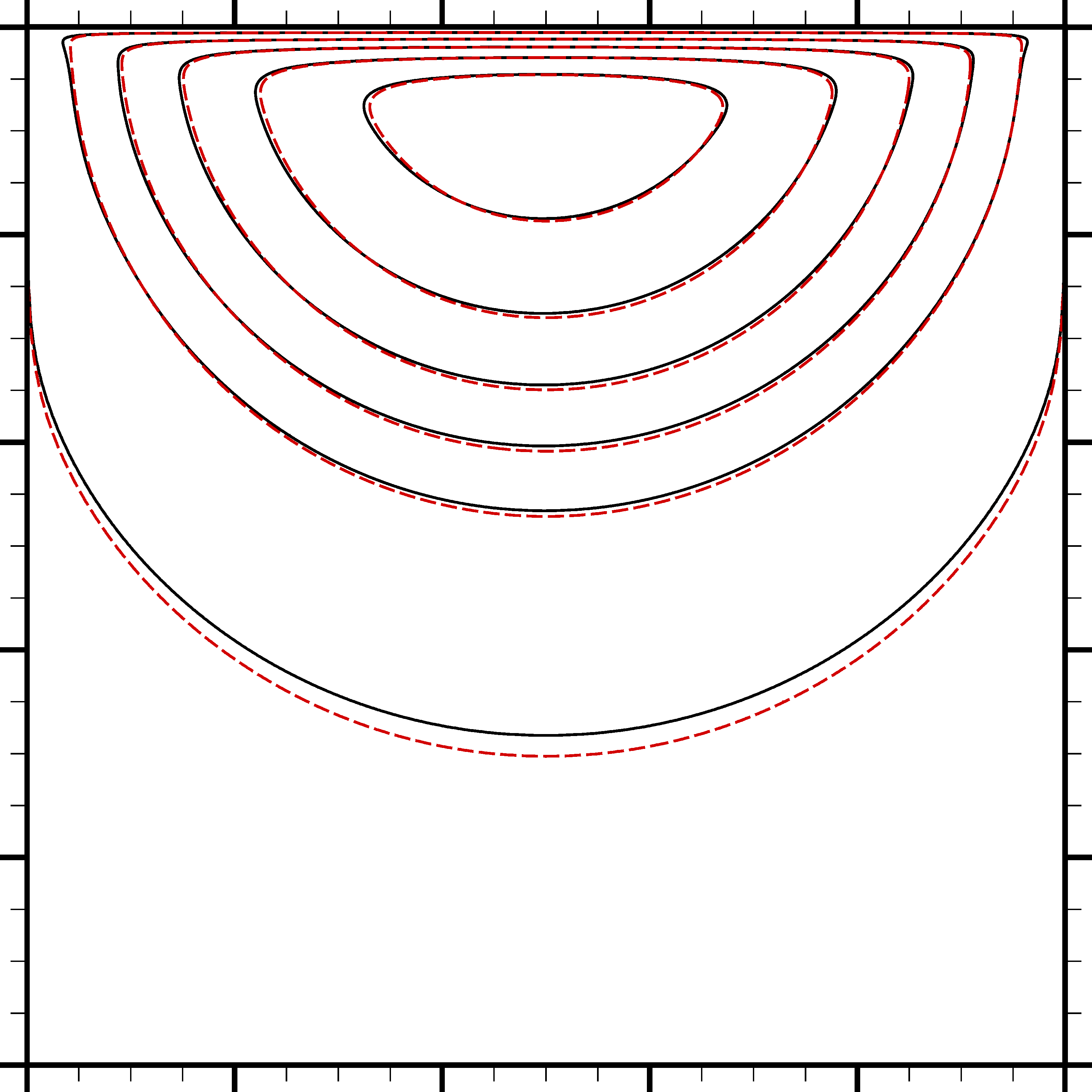
(b) $G=4,000$ $\mathrm{P}\mathrm{a}$

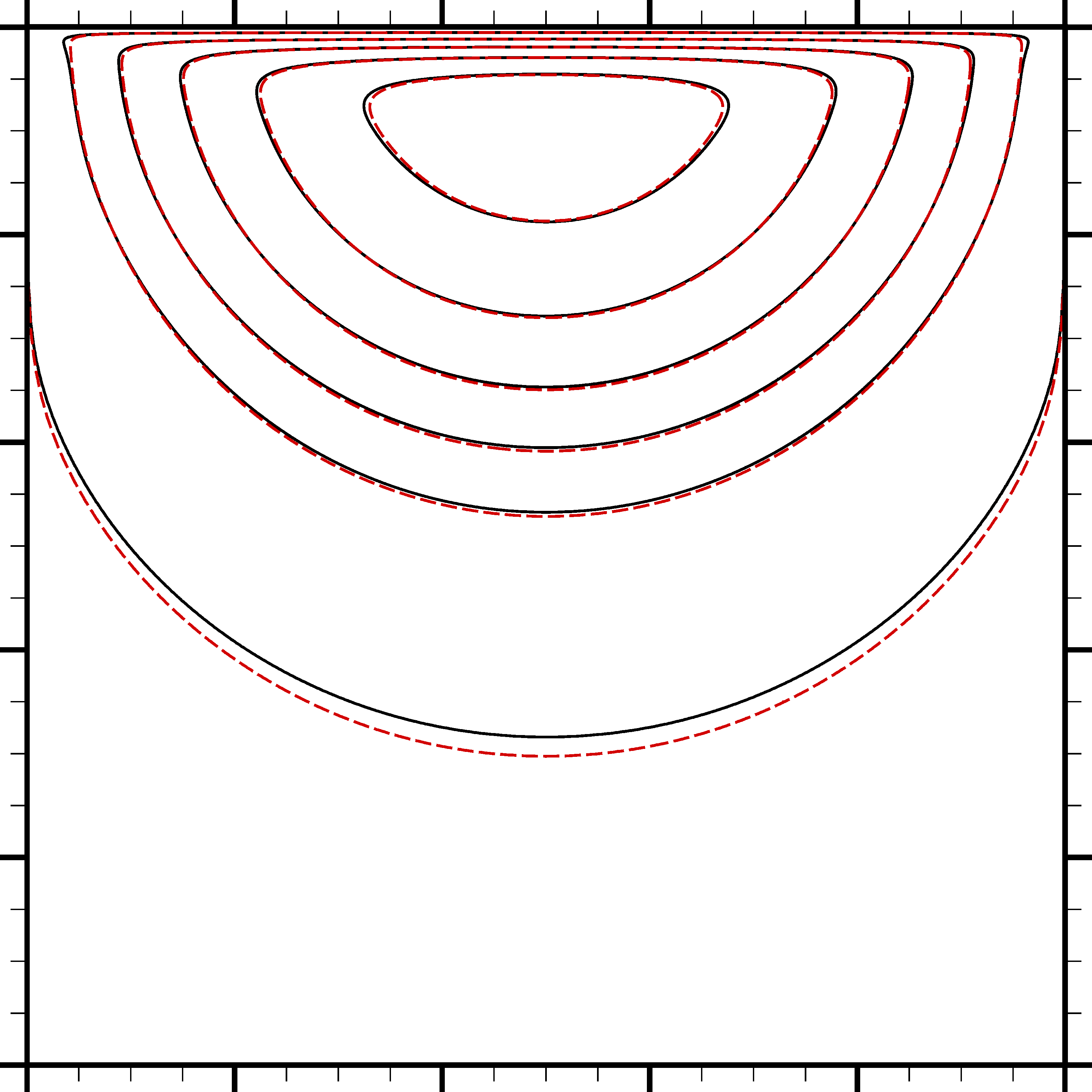
(c) $G=40,000$ $\mathrm{P}\mathrm{a}$

Figure 16: Continuous lines: SHB streamlines for various values of $G$, as indicated (the rest of the parameters are as in Table 2, and the lid velocity is $U$ = 0.1 $\mathrm{m}\mathrm{/}\mathrm{s}$). Dashed lines: corresponding HB streamlines, drawn at the same streamfunction values as for the SHB model. Since the HB predictions are independent of $G$, the dashed lines do not change between plots. The streamlines are drawn at fixed streamfunction intervals.

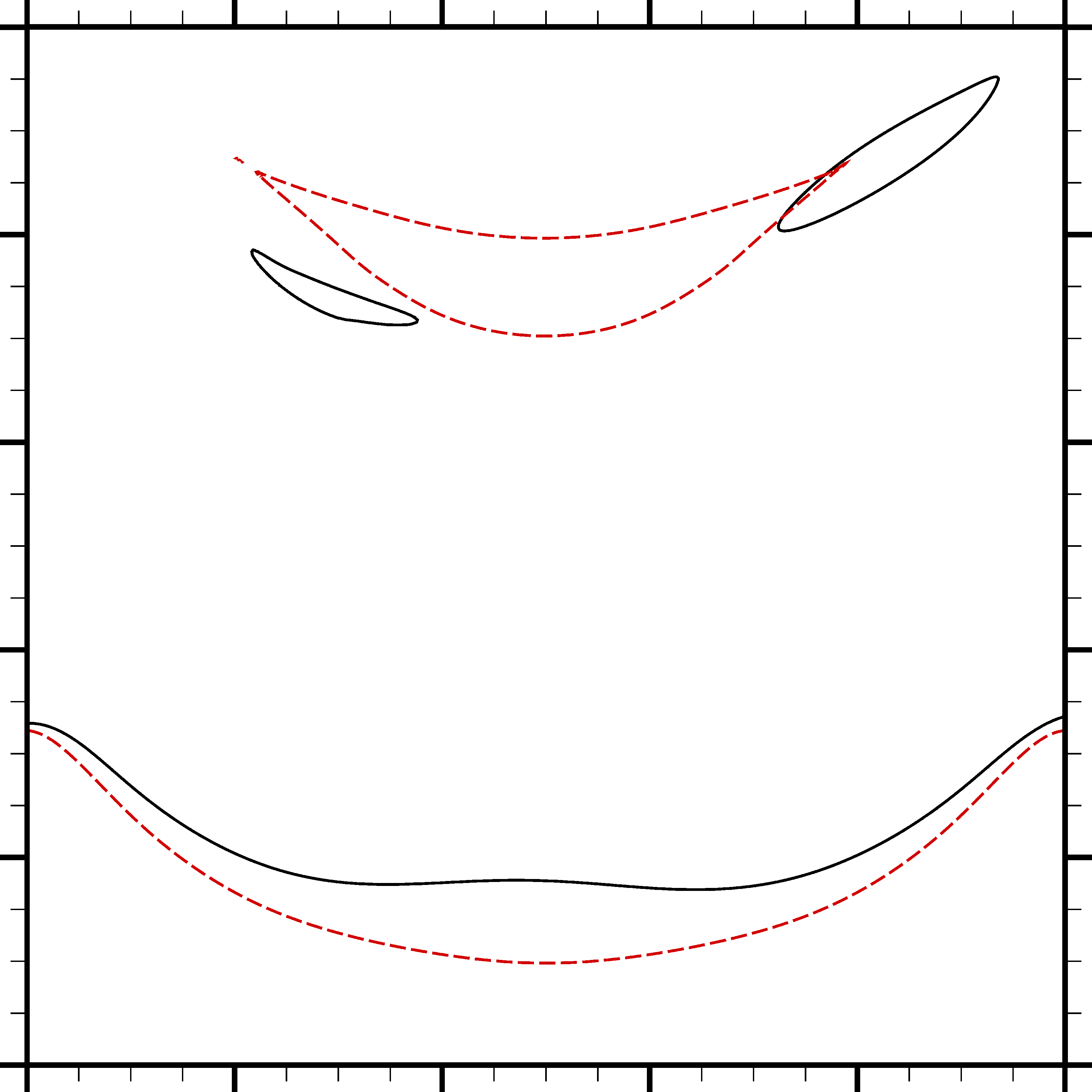
(a) $\tau_{d}=40$ $\mathrm{P}\mathrm{a}$; $G=400$ $\mathrm{P}\mathrm{a}$

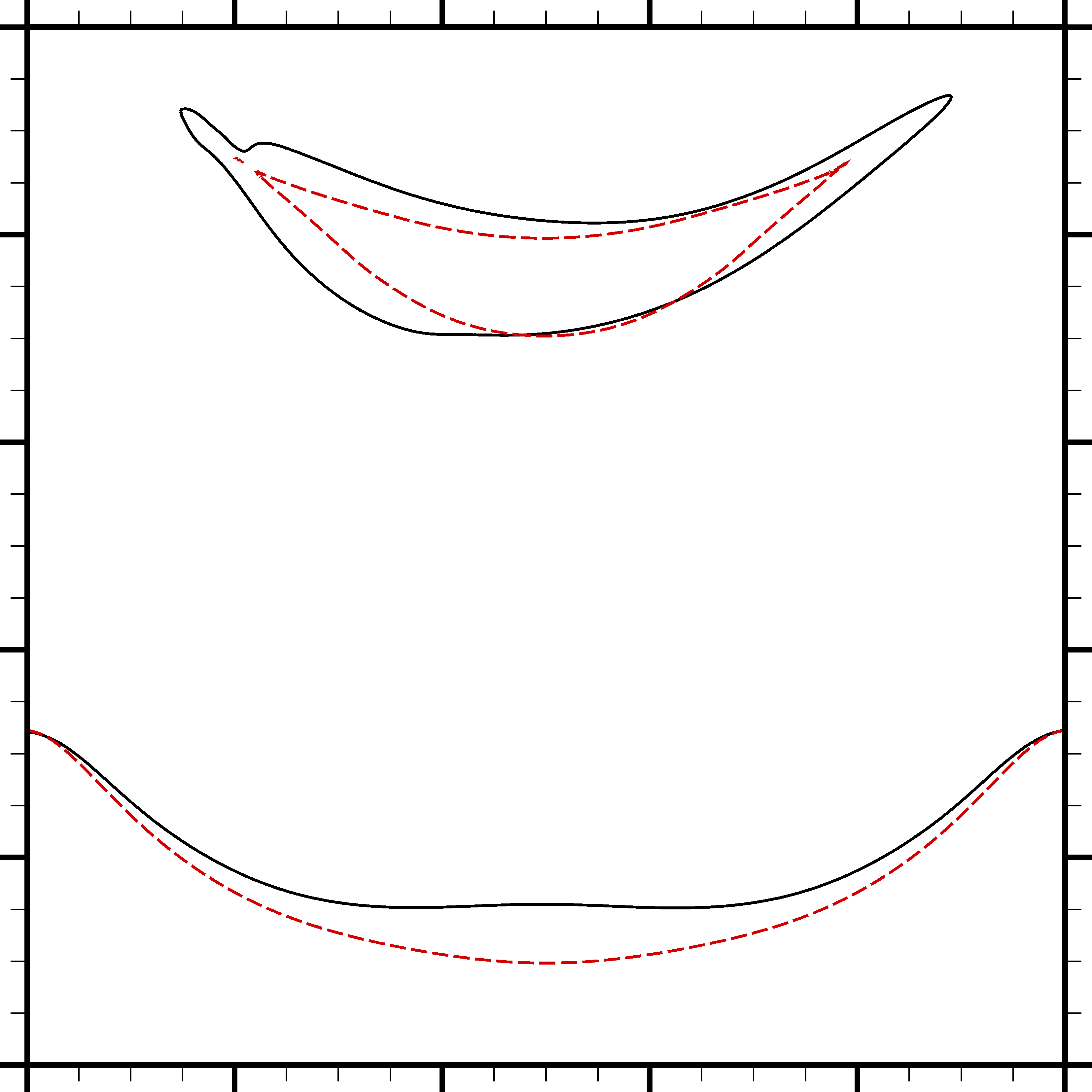
(b) $\tau_{d}=40$ $\mathrm{P}\mathrm{a}$; $G=4,000$ $\mathrm{P}\mathrm{a}$

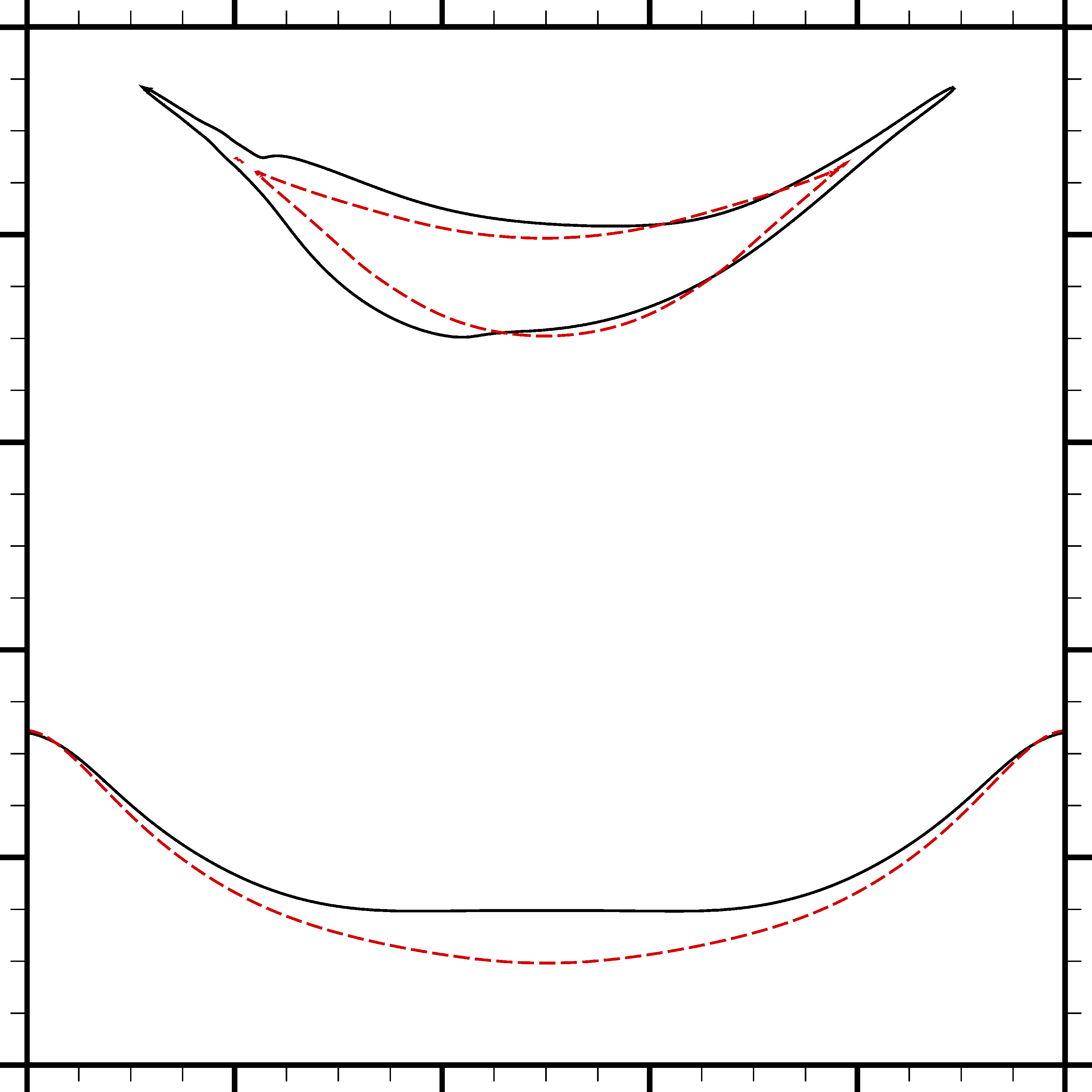
(c) $\tau_{d}=40$ $\mathrm{P}\mathrm{a}$; $G=40,000$ $\mathrm{P}\mathrm{a}$

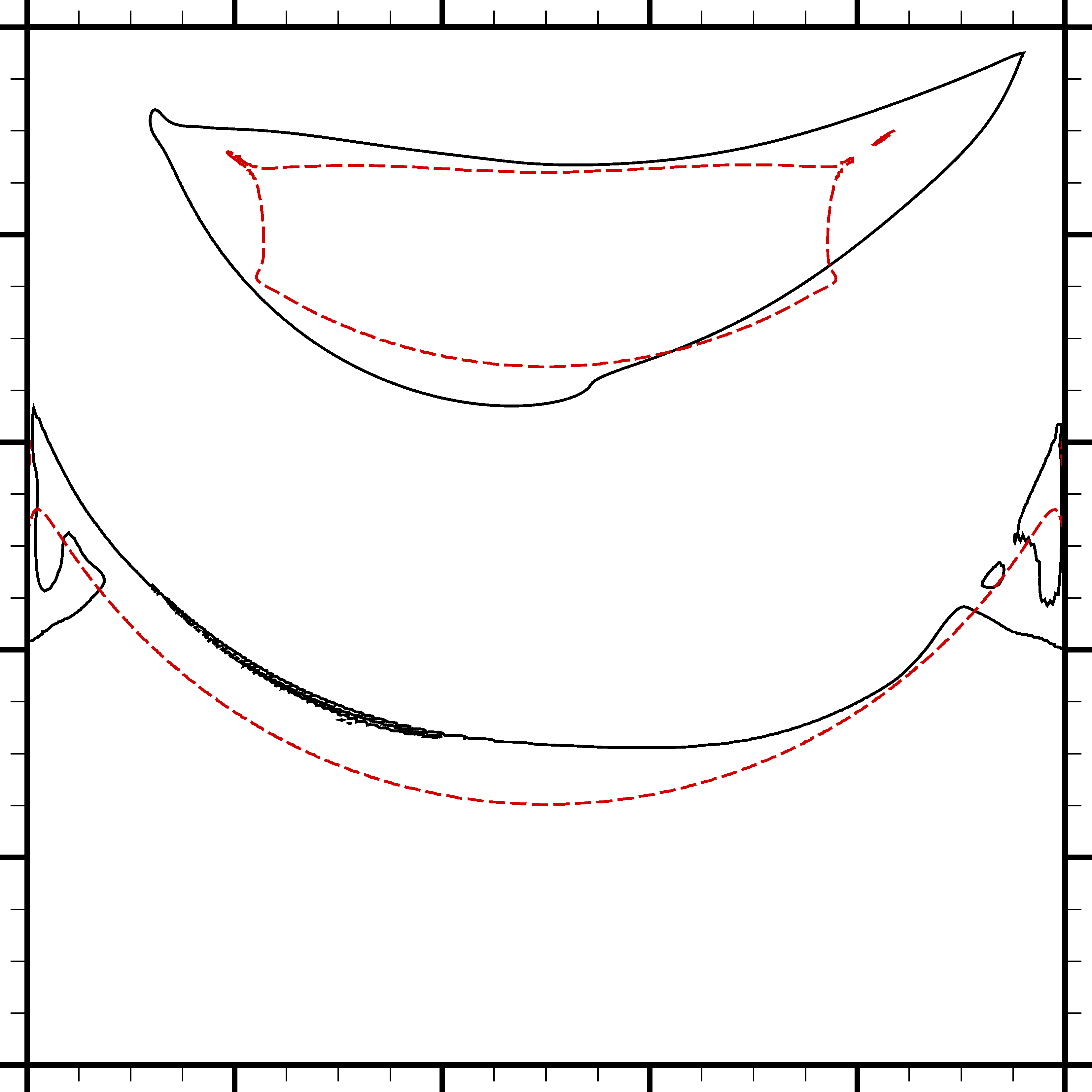
(d) $\tau_{d}=70$ $\mathrm{P}\mathrm{a}$; $G=400$ $\mathrm{P}\mathrm{a}$

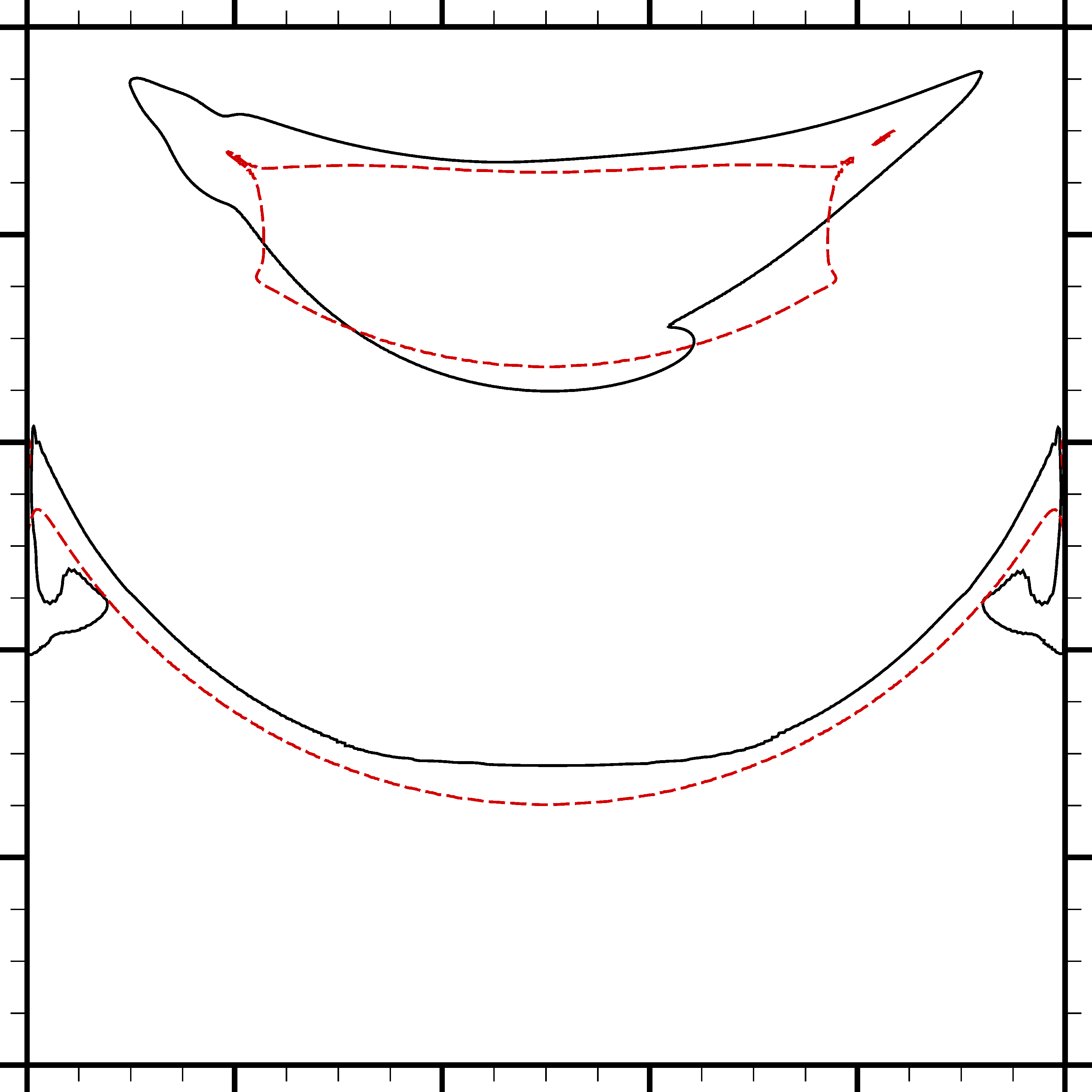
(e) $\tau_{d}=70$ $\mathrm{P}\mathrm{a}$; $G=4,000$ $\mathrm{P}\mathrm{a}$

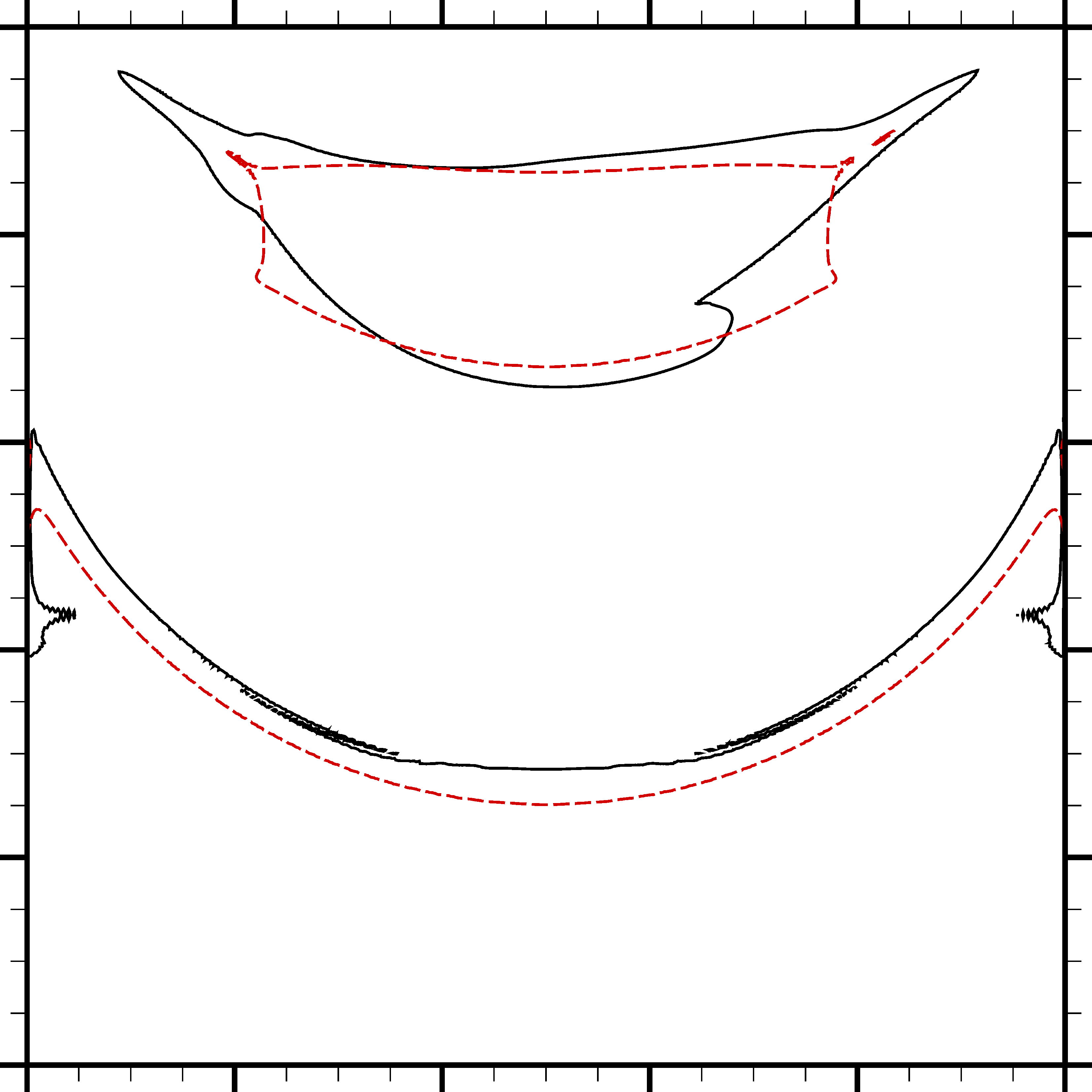
(f) $\tau_{d}=70$ $\mathrm{P}\mathrm{a}$; $G=40,000$ $\mathrm{P}\mathrm{a}$

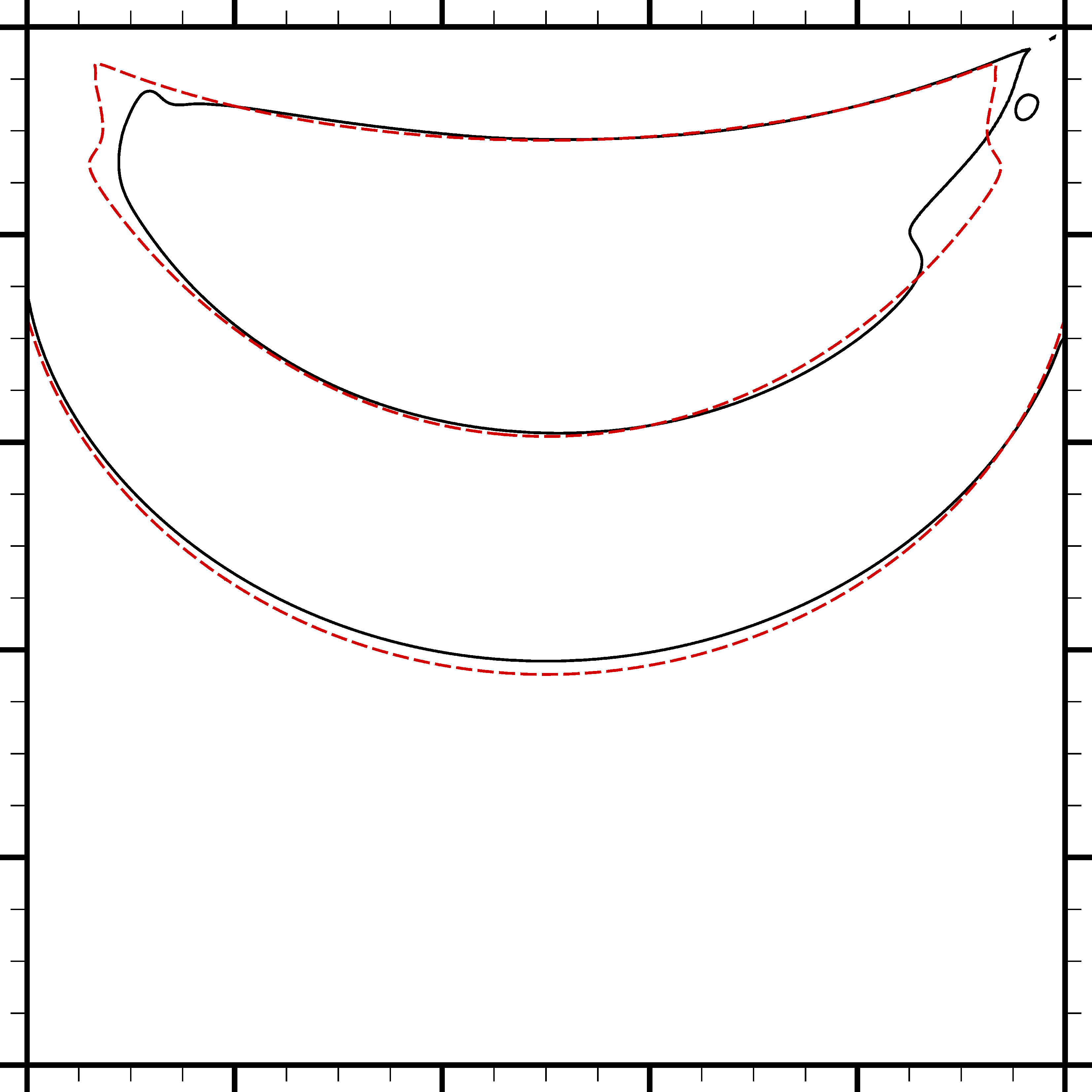
(g) $\tau_{d}=80$ $\mathrm{P}\mathrm{a}$; $G=400$ $\mathrm{P}\mathrm{a}$

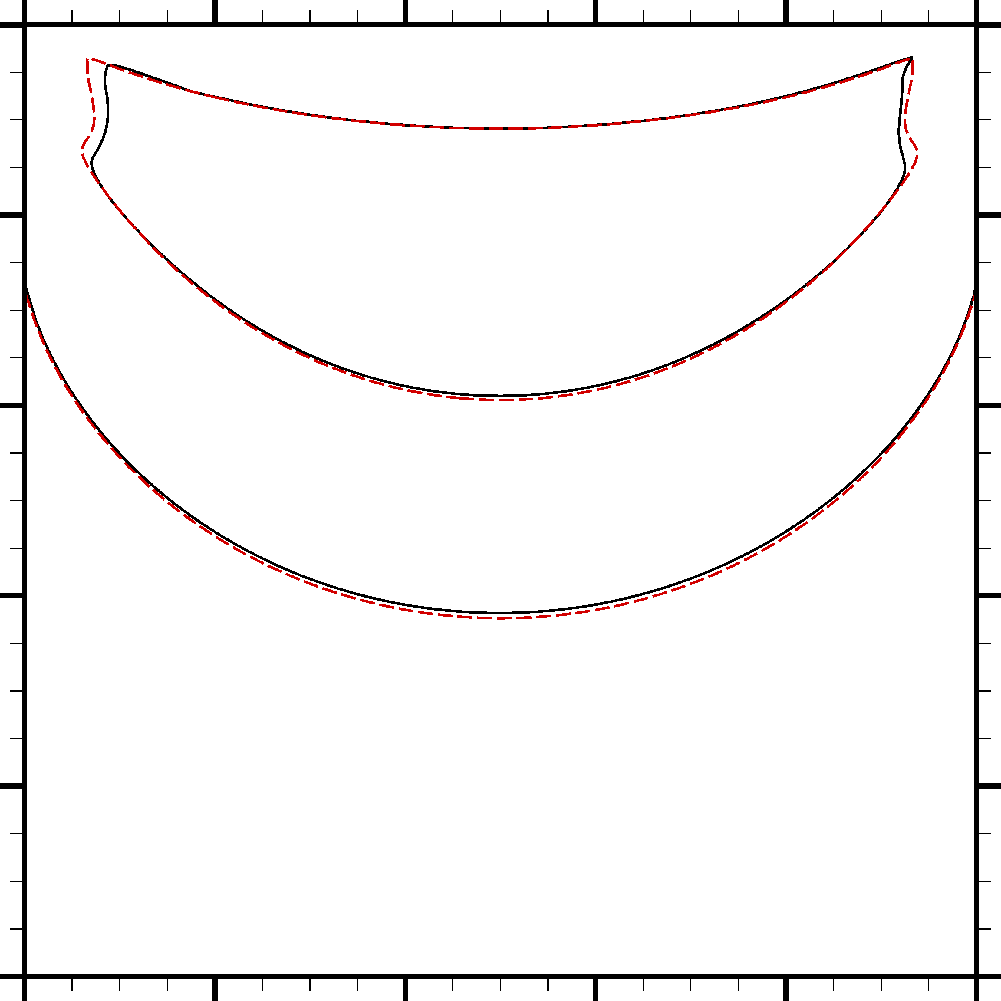
(h) $\tau_{d}=80$ $\mathrm{P}\mathrm{a}$; $G=4,000$ $\mathrm{P}\mathrm{a}$

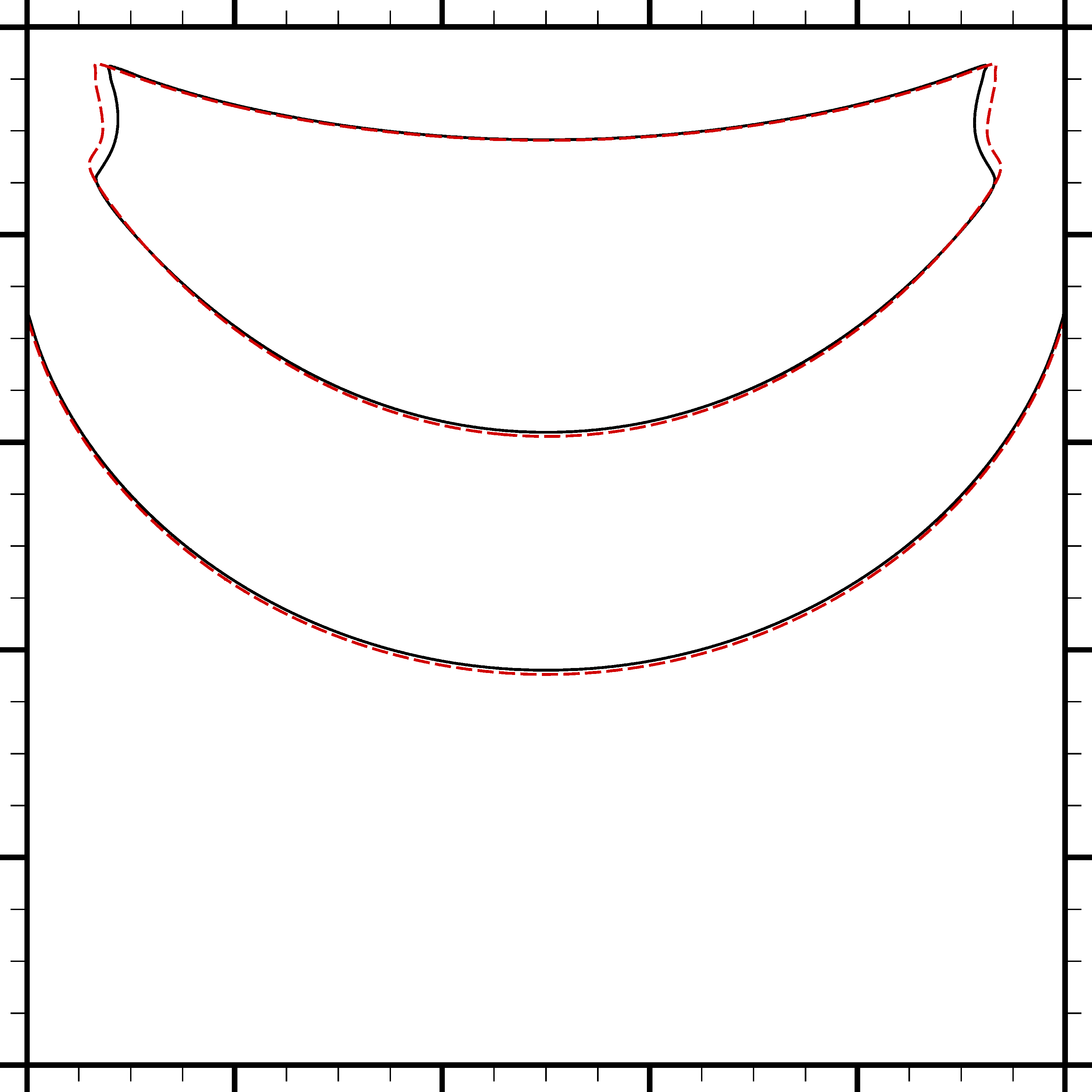
(i) $\tau_{d}=80$ $\mathrm{P}\mathrm{a}$; $G=40,000$ $\mathrm{P}\mathrm{a}$

Figure 17: Continuous lines: contours of $\tau_{d}$ predicted by the SHB model (top row: $\tau_{d}$ = 40 $\mathrm{P}\mathrm{a}$; middle row: $\tau_{d}=\tau_{y}$ = 70 $\mathrm{P}\mathrm{a}$; bottom row: $\tau_{d}$ = 80 $\mathrm{P}\mathrm{a}$) for various values of the elastic modulus $G$ (left column: $G$ = 400 $\mathrm{P}\mathrm{a}$; middle column: $G$ = 4,000 $\mathrm{P}\mathrm{a}$; right column: $G$ = 40,000 $\mathrm{P}\mathrm{a}$), the rest of the parameters having the values listed in Table 2, and the lid velocity being $U$ = 0.1 $\mathrm{m}\mathrm{/}\mathrm{s}$. Dashed lines: corresponding contours predicted by the HB model.

6.4 A case with slip

Carbopol gels are quite slippery [11, 78, 74]; the previous, no-slip results can be considered to correspond to roughened walls, like those used in rheological measurements to avoid slip [33]. However, if the walls are smooth then noticeable slip is expected. Viscoplastic and viscoelastic fluids can exhibit complex slip behaviour, e.g. power-law slip [79, 80], pressure dependence [81], or “slip yield stress” [82, 83]. However, experiments with Carbopol in [78] (0.2% by weight) and [74] (0.08% by weight) showed nearly Navier slip behaviour, $u_{s}=5.151\times 10^{-4}\,\tau_{w}^{0.876}$ and $u_{s}=2.3\times 10^{-4}\,\tau_{w}^{1.32}$, respectively, where $u_{s}$ is the slip velocity (the left-hand side of Eq. (11)) and $\tau_{w}$ is the wall tangential stress (the term $(\underline{n}\cdot\underline{\underline{\tau}})\cdot\underline{s}$ of the right-hand side of Eq. (11)). In [74] it is conjectured that this may be due to the formation of a thin layer of Newtonian fluid (solvent) that separates the wall surface from the gel micro-particles. In the present section we impose a Navier slip condition, Eq. (11), on all walls, with a slip coefficient $\beta=5\times 10^{-4}$ $\mathrm{m}\mathrm{/}\mathrm{P}\mathrm{a}\,\mathrm{s}$. For this case, concerning stress extrapolation to the walls, we could not get SIMPLE to converge with the $D$ coefficients given by (46) – (47) and we set them equal to zero.

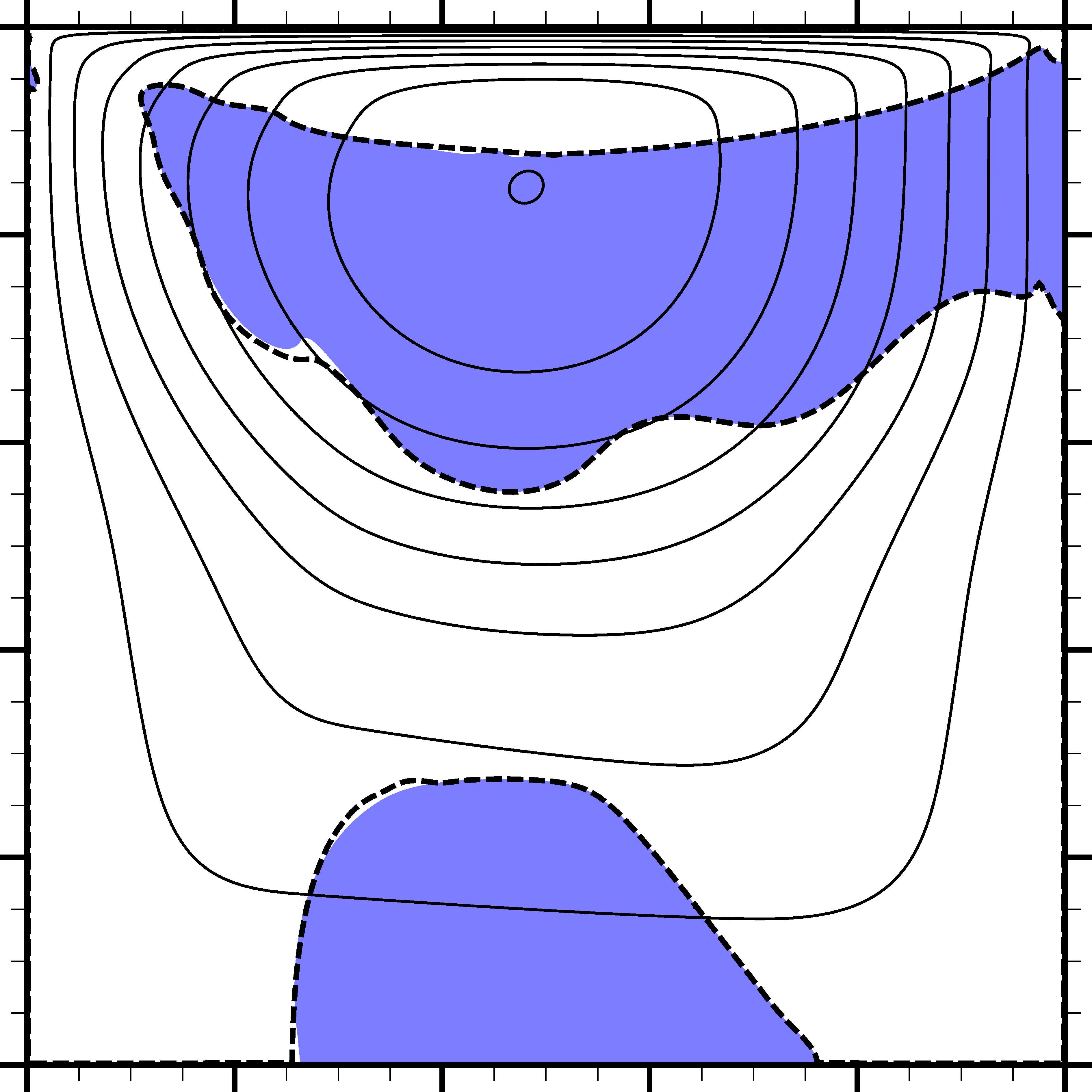
(a) SHB flowfield

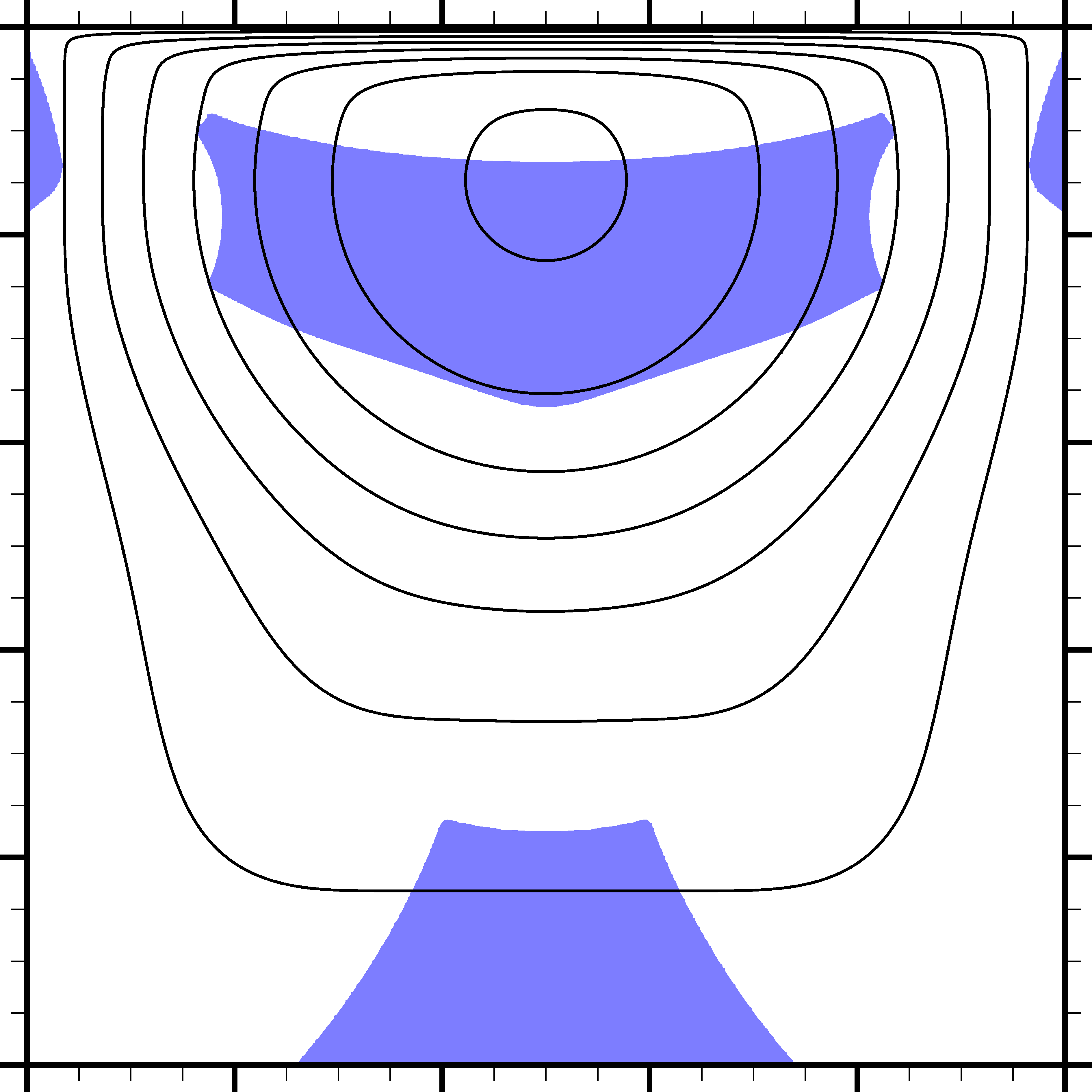
(b) HB flowfield

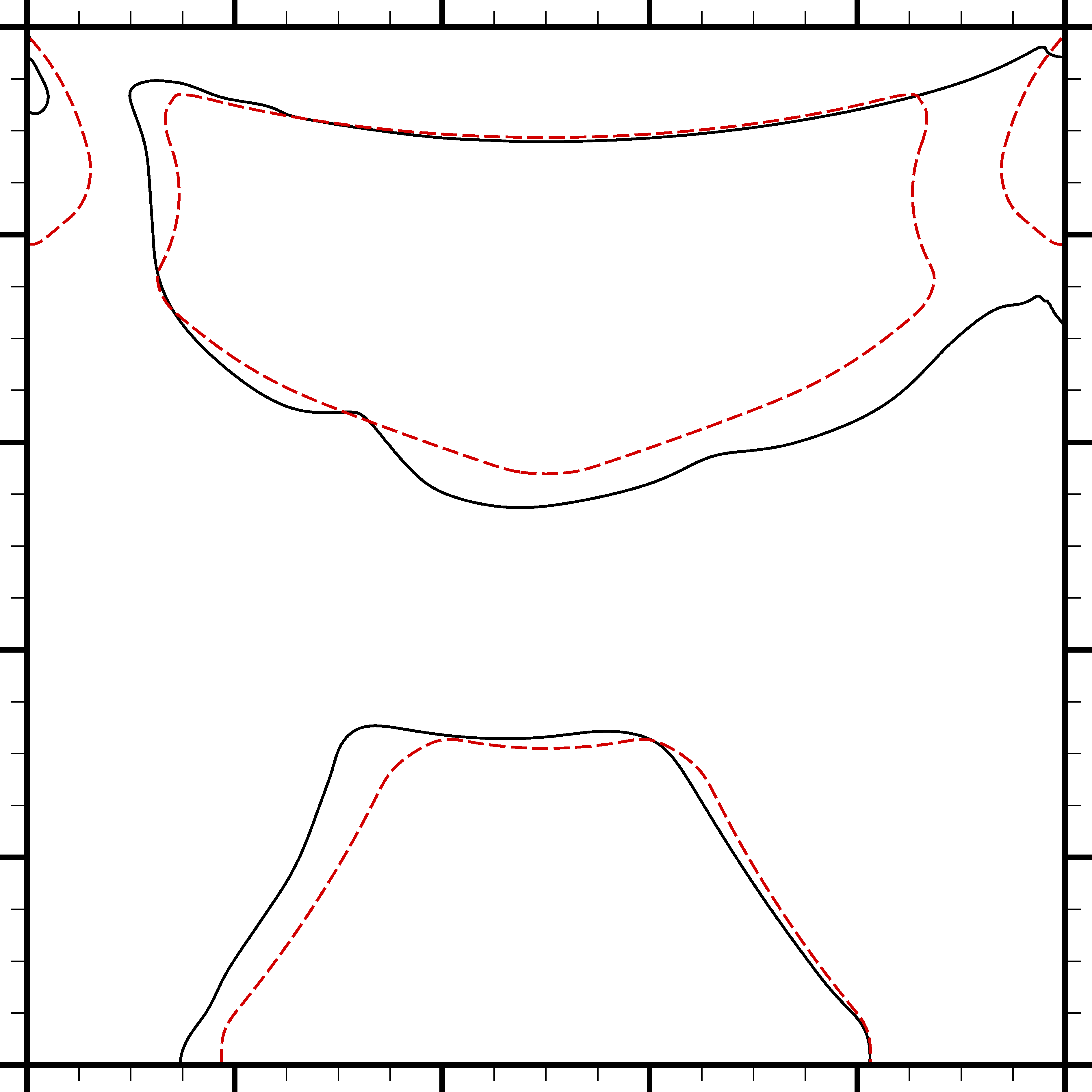
(c) $\tau_{d}$ = 75 $\mathrm{P}\mathrm{a}$

Figure 18: 18(a) SHB flowfield for the slip case; shaded region: unyielded material at $t$ = 60 $\mathrm{s}$; dashed lines: yield lines at $t$ = 30 $\mathrm{s}$; continuous lines: streamlines (they are drawn at equal streamfunction intervals). 18(b) Corresponding steady-state HB flowfield (the streamlines are drawn at the same values of streamfunction as in 18(a)). 18(c) The $\tau_{d}$ = 75 $\mathrm{P}\mathrm{a}$ contour of the SHB (continuous line) and HB (dashed line) flowfields.

Figure 18(a) shows the flowfield. A distinguishing feature is that the two unyielded zones touch the cavity walls and yet contain moving material which is sliding over the wall. This feature is common also to the HB flowfield, shown in Fig. 18(b), which is, again, much more symmetric. Figure 18(c) shows that SHB and HB contours of $\tau_{d}$ are more similar for $\tau_{d}>\tau_{y}$. Due to slip, the flow induced by the lid is much weaker than in the no-slip case, as can be seen from the lower kinetic energy in Fig. 10, the smaller vortex strength in Table 4, and the wider streamline spacing in Fig. 19(b) than in Fig. 19(a). On the other hand, the streamlines in Fig. 19(b) are more evenly spaced near the bottom of the cavity compared to Fig. 19(a) as slip allows the circulation to extend all the way down to the bottom wall, where now there is no stationary unyielded zone. Consequently, there is also no transition zone. Indeed, comparing in Fig. 18(a) the yield lines at $t$ = 30 $\mathrm{s}$ (dashed lines) and $t$ = 60 $\mathrm{s}$ (the boundary of the shaded regions) one sees that there is very little change, and the bottom unyielded zone even slightly contracts with time. The absence of a transition zone can be explained by examining the $\dot{\gamma}$ distributions of Fig. 19; whereas in the no-slip case (Fig. 19(a)) the velocity gradients are practically zero inside the bottom unyielded zone, in the slip case (Fig. 19(b)) they are non-zero throughout the domain, thus excluding the transition zone situation where the constitutive equation reduces to Eq. (71). Figure 19 also shows that in the upper part of the cavity $\dot{\gamma}$ is much lower in the presence of slip. Due to the shear-thinning nature of the fluid, this results in higher viscosities and associated relaxation times which may explain why the stress evolution is slower in the slip case than in the no-slip one as seen in Fig. 10(b) (and also in Figs. 18(a) and 20, where there are slight changes between $t$ = 30 and 60 $\mathrm{s}$). Surprisingly, Fig. 10(b) shows that $\mathrm{tr}(\underline{\underline{\tau}})_{\mathrm{avg}}$ is actually higher in the slip case, probably due to the absence of a bottom stationary zone. For benchmarking purposes we plot profiles of some dependent variables along the vertical centreline in Fig. 20.

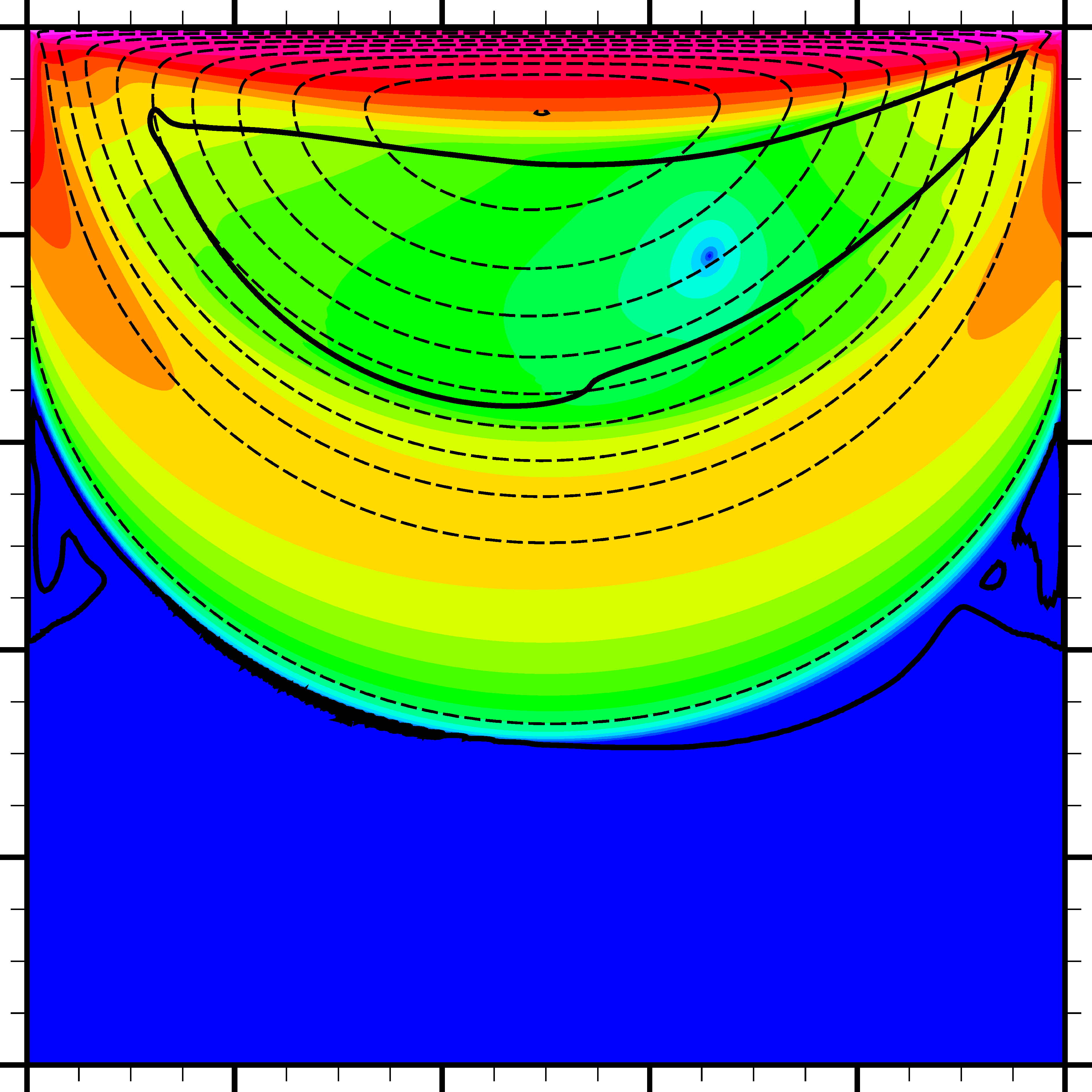
(a) No slip

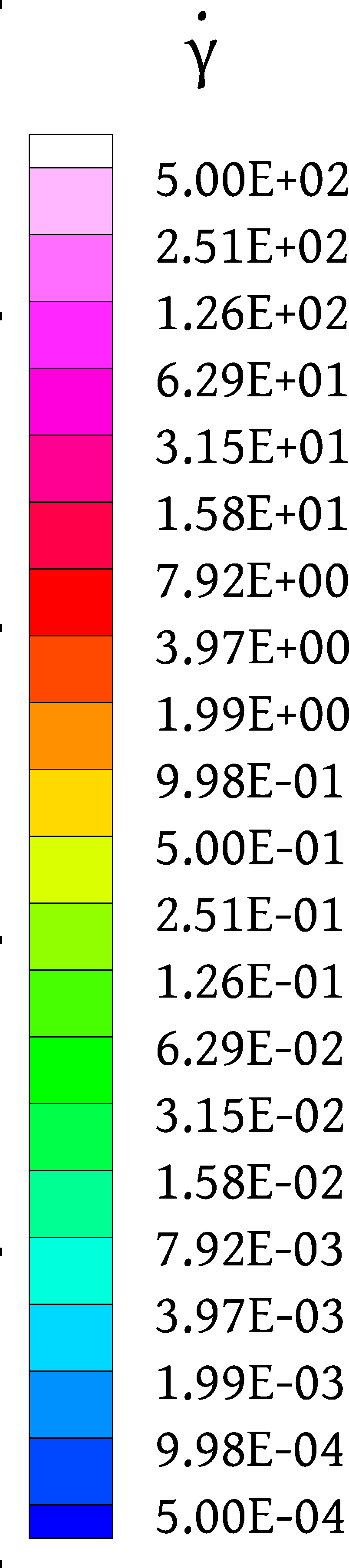
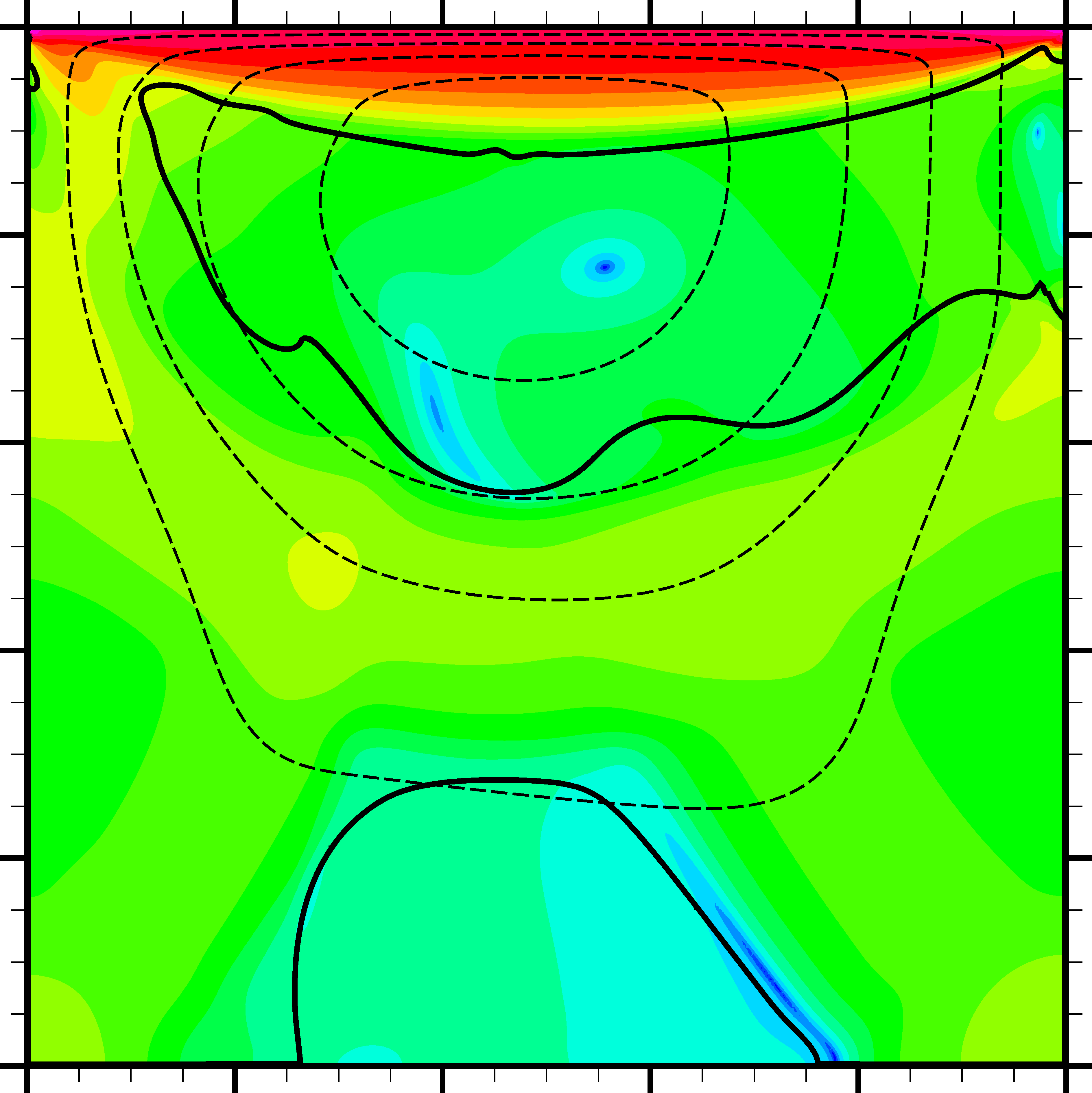
(b) Slip

Figure 19: Contours of $\dot{\gamma}$ [$\mathrm{s}^{-1}$] for $U$ = 0.100 $\mathrm{m}\mathrm{/}\mathrm{s}$ without wall slip 19(a) (base case) or with wall slip 19(b). The thick continuous lines are yield lines and the dashed lines are streamlines. The latter are plotted at equal streamfunction intervals (the same intervals in both figures).

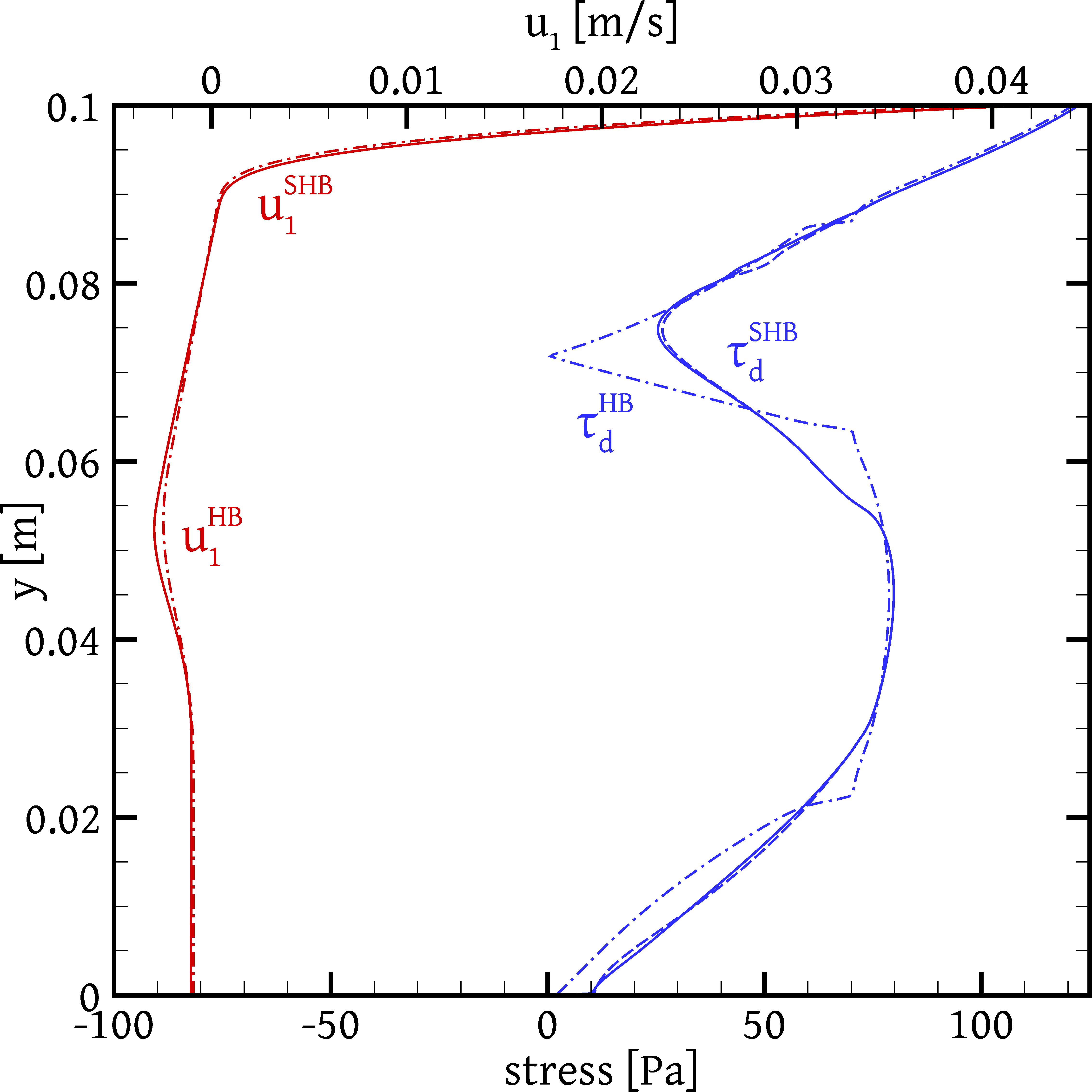
(a) $u_{1}$ and $\tau_{d}$ at $x=L/2$

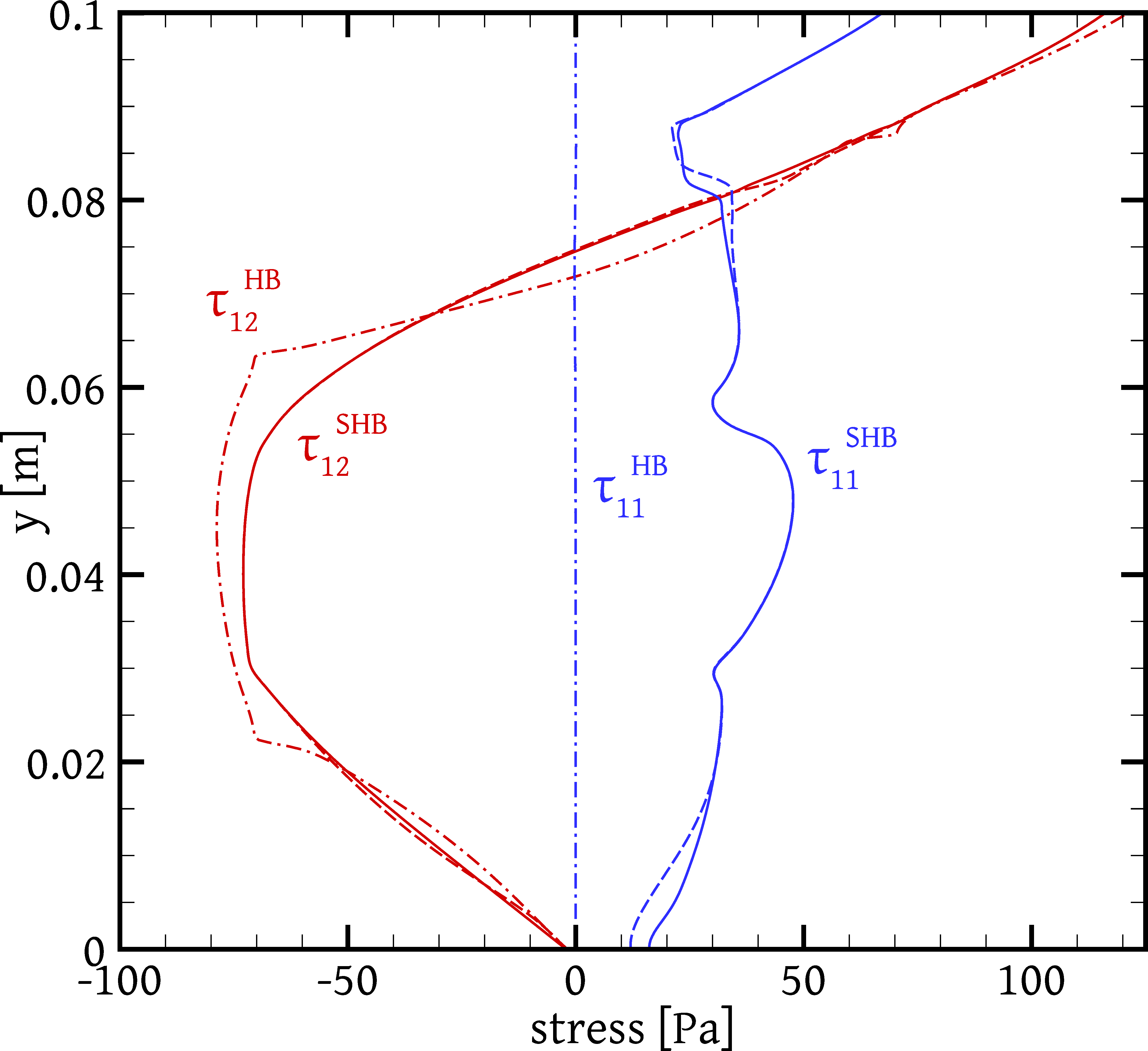
(b) $\tau_{11}$ and $\tau_{12}$ at $x=L/2$

Figure 20: Profiles of some dependent variables along the vertical centreline, for the slip case. SHB results at $t$ = 60 and 30 $\mathrm{s}$ are plotted in continuous and dashes lines, respectively, and steady state HB results in dash-dot line.

6.5 Multiplicity of solutions

It was mentioned in Sec. 2 that Cheddadi et al. [32] found that the steady state of a SHB flow (including the velocity field) can depend in a continuous manner on the initial conditions. That was observed in simple cylindrical Couette flow, where the shear stress is determined by the geometry and kinematics but the circumferential normal stress depends also on its initial value, which affects the final extent of the yield zone and therefore also the final velocity field. We performed analogous experiments to see if this can be observed also in the present, more complex flow. So, we solved two more cases that are identical to the “base case” of Sec. 6.1, except for the initial stress conditions: $\tau_{11}=\tau_{22}=+\sqrt{3}\tau_{y}$ (first case) or $-\sqrt{3}\tau_{y}$ (second case) throughout, the remaining stress components being zero. These initial conditions correspond, respectively, to tension and compression states that are isotropic in the $xy$ plane; from Eq. (9) it follows that $\tau_{d}(t=0)=\tau_{y}$ everywhere, i.e. the material is on the verge of yielding. The material is initially at rest ($\underline{u}=0$). The simulations were carried on until time $t$ = 60 $\mathrm{s}$.

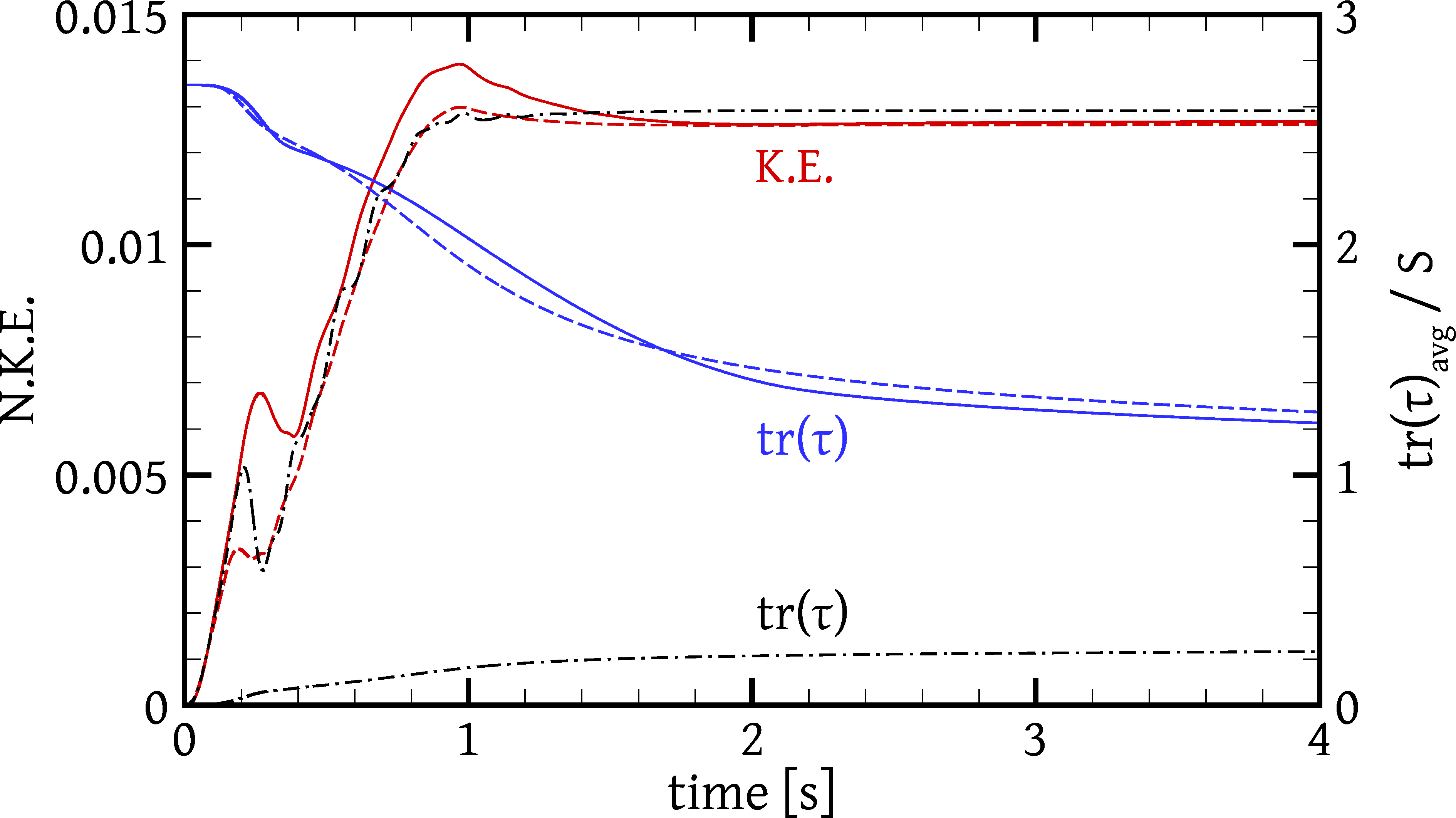
(a) $t\in[0,4]$ $\mathrm{s}$

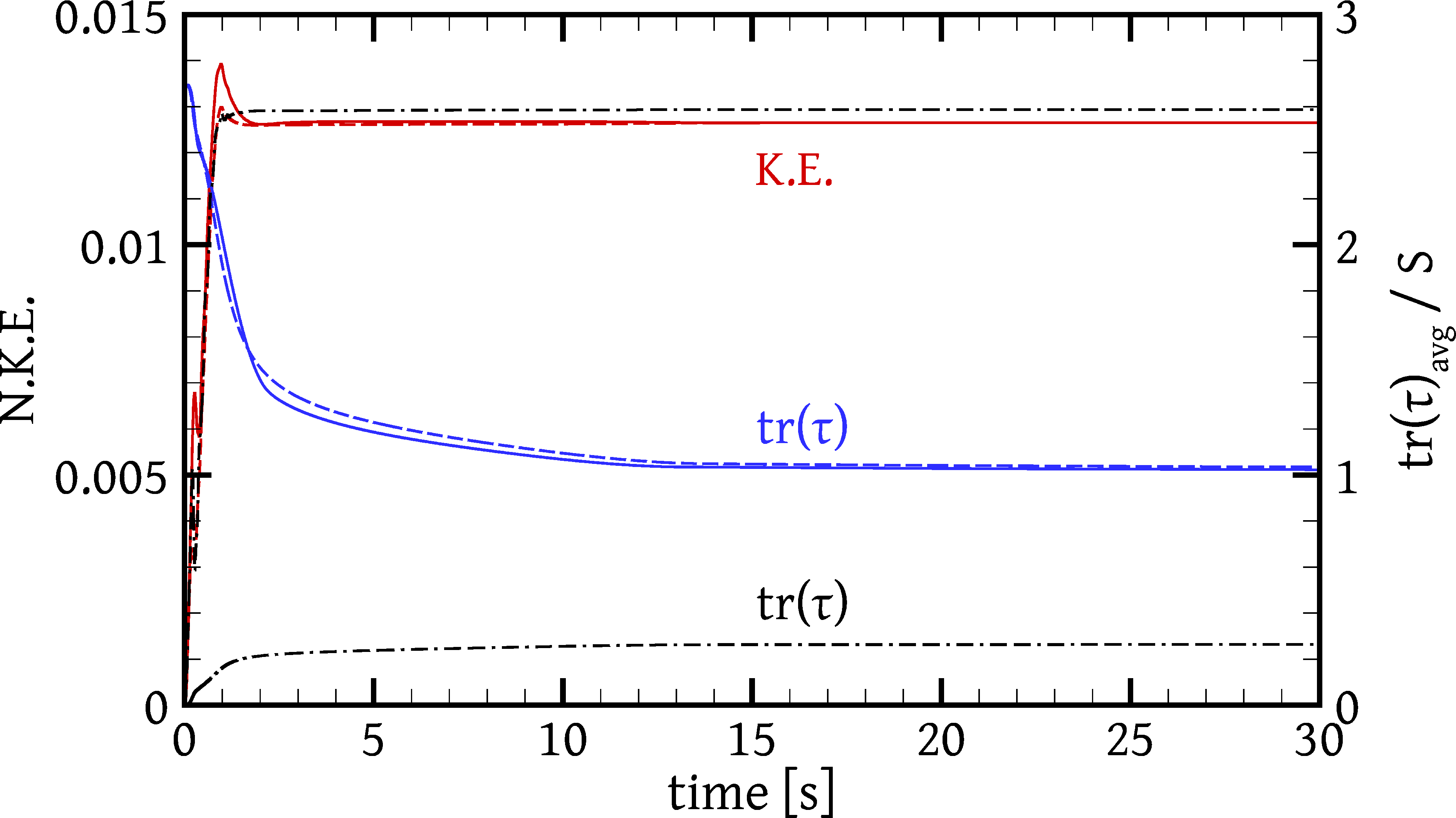
(b) $t\in[0,30]$ $\mathrm{s}$

Figure 21: Histories of N.K.E. (Eq. (69)) and $\mathrm{tr}(\underline{\underline{\tilde{\tau}}})_{\mathrm{avg}}$ (Eq. (70)) for the cases with initial conditions $\tau_{11}=\tau_{22}=-\sqrt{3}\tau_{y}$ (continuous lines), $\tau_{11}=\tau_{22}=+\sqrt{3}\tau_{y}$ (dashed lines) and $\tau_{11}=\tau_{22}=0$ (dash-dot lines, the base case).

Interestingly, the velocity fields of both of these new cases arrive at practically the same steady state; this can be seen in Fig. 21, where the kinetic energies of both cases converge, and more clearly in Fig. 22(a) where the respective streamlines can be seen to be identical. However, this steady-state is not the same as that arrived at in the base case ($\tau_{11}=\tau_{22}=0$); Fig. 21 shows that unlike in the two new cases, the kinetic energy of the base case does not exhibit an overshoot and eventually increases to a value which is about 2.25% larger than that of the other two cases. In Fig. 22(a) the base case streamlines are also not identical to those of the other two cases. As far as the main vortex is concerned, the new cases have it located at $(\tilde{x}_{c},\tilde{y}_{c})=(0.497,0.917)$ with a strength of $\tilde{\psi}_{c}=-0.0266$, which is located slightly to the right and is slightly weaker than that of the base case (Table 4). Of course, all these differences are small, but nevertheless they confirm the observation of Cheddadi et al. [32].

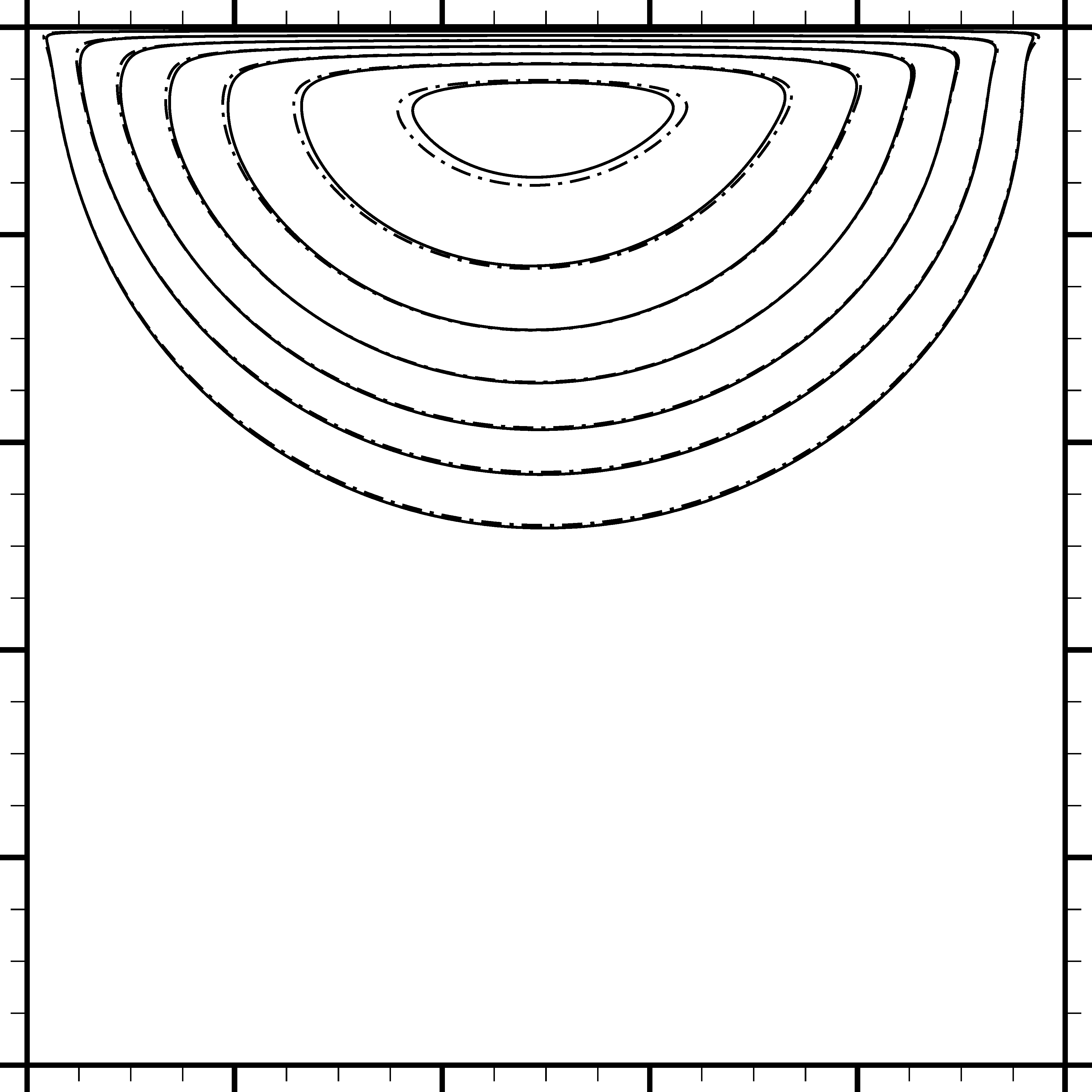
(a) streamlines

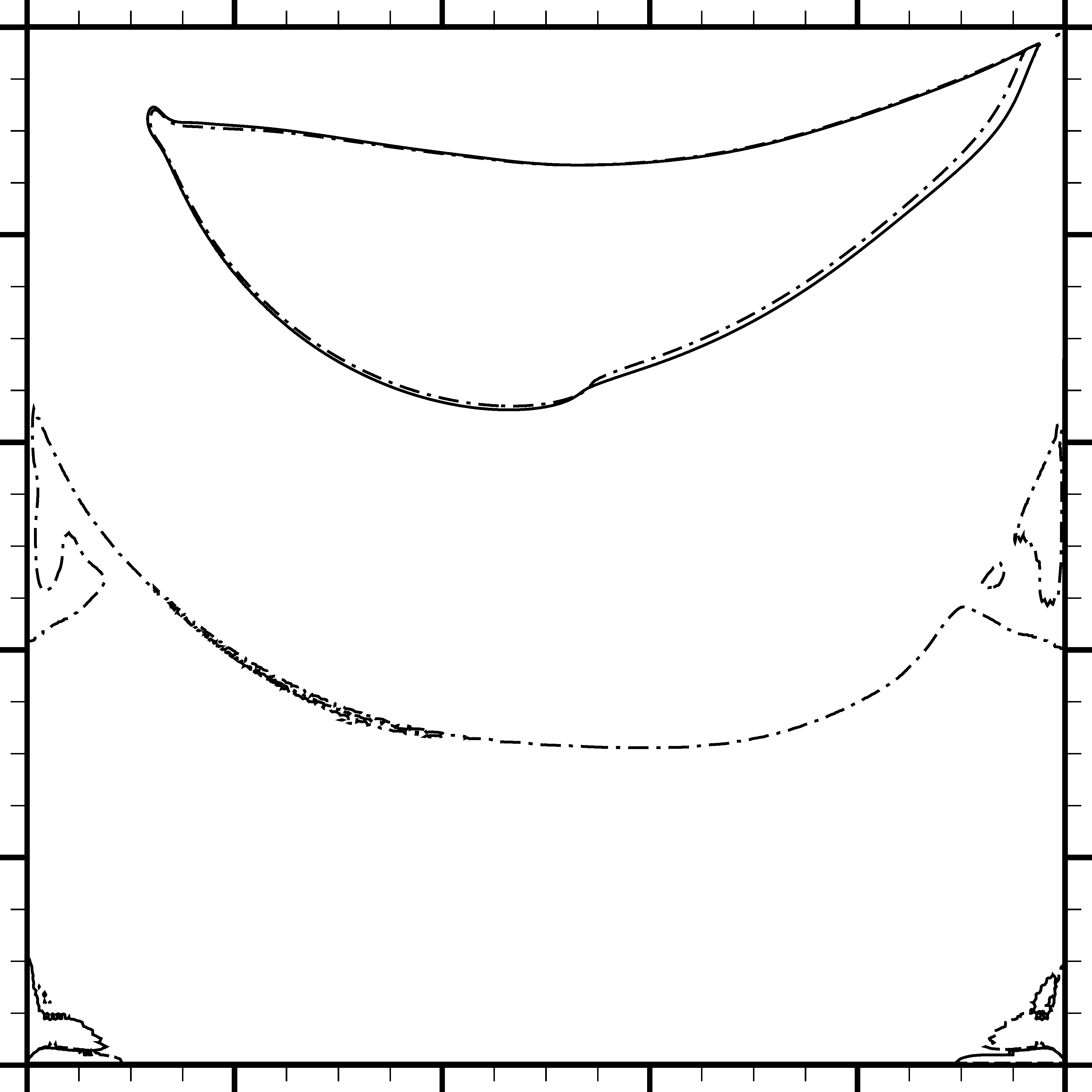
(b) yield lines

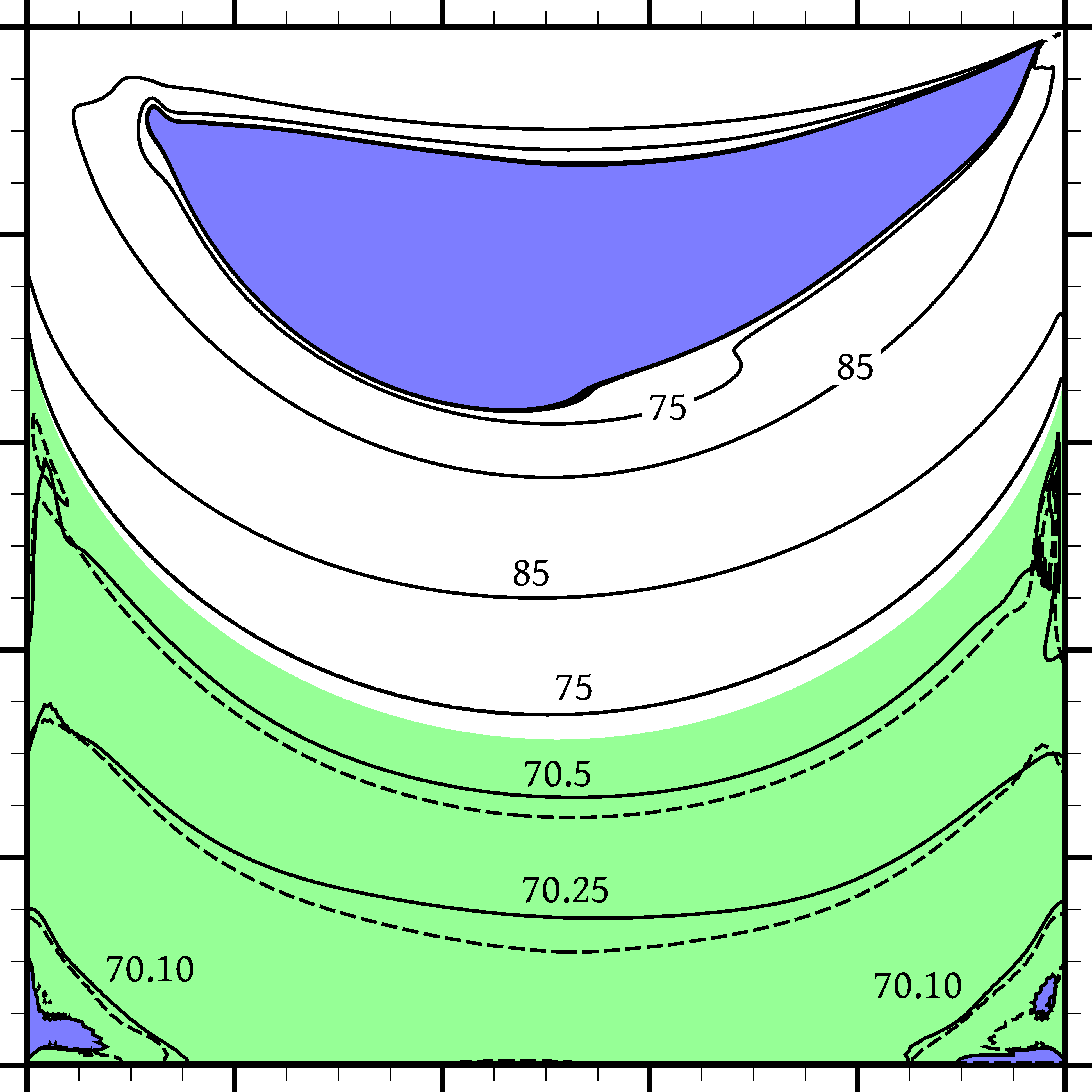
(c) $\tau_{d}$

Figure 22: Steady-state streamlines 22(a) (streamfunction interval $\delta\phi/(\rho U)$ = $3.6\text{\times}{10}^{-4}$), yield lines 22(b), and $\tau_{d}$ contours 22(c) for the cases with initial conditions $\tau_{11}=\tau_{22}=-\sqrt{3}\tau_{y}$ (continuous lines), $+\sqrt{3}\tau_{y}$ (dashed lines), and zero (dash-dot lines, only in 22(a) and 22(c)). In 22(c) the values of $\tau_{d}$, in $\mathrm{P}\mathrm{a}$, are indicated next to each contour. The unyielded region of the $\tau_{11}=\tau_{22}=-\sqrt{3}\tau_{y}$ case is shaded blue. The region where $\|\underline{u}\|<5\times 10^{-5}U$ is shaded green.

Concerning the stress fields, we can note the following. Firstly, a striking difference between the new cases and the base case is that in the former the bottom unyielded zone is largely absent and is replaced by a large transition zone; this is shown in Fig. 22(c) where the transition zone is approximately the green region, throughout which $\tau_{d}$ is slightly above $\tau_{y}$. Inside the transition region the $\tau_{d}$ fields of the two new cases are similar (Fig. 22(c)), but the individual $\tau_{11}$ and $\tau_{22}$ stress components have opposite signs which they have inherited from the initial conditions, as seen in Fig. 23; in fact, near the bottom wall these stress components retain values close to the initial ones, $\pm\sqrt{3}\tau_{y}\approx 121$ $\mathrm{P}\mathrm{a}$. On the other hand, the base case stresses are close to zero in that region, again an inheritance of the initial conditions. This reflects on the much lower stress trace values seen in Fig. 21. Outside of the transition region, where the rates of deformation are non-zero (including the plug zone), the two new cases have identical steady-state stress fields, as seen in Figs. 22(c) and 23, whereas those of the base case deviate slightly. This includes the yield line that forms the boundary of the plug zone: Fig. 22(b) shows that the plug zones of the two new cases are identical, but that of the base case is slightly smaller, which is likely the cause of the slightly different velocity field.

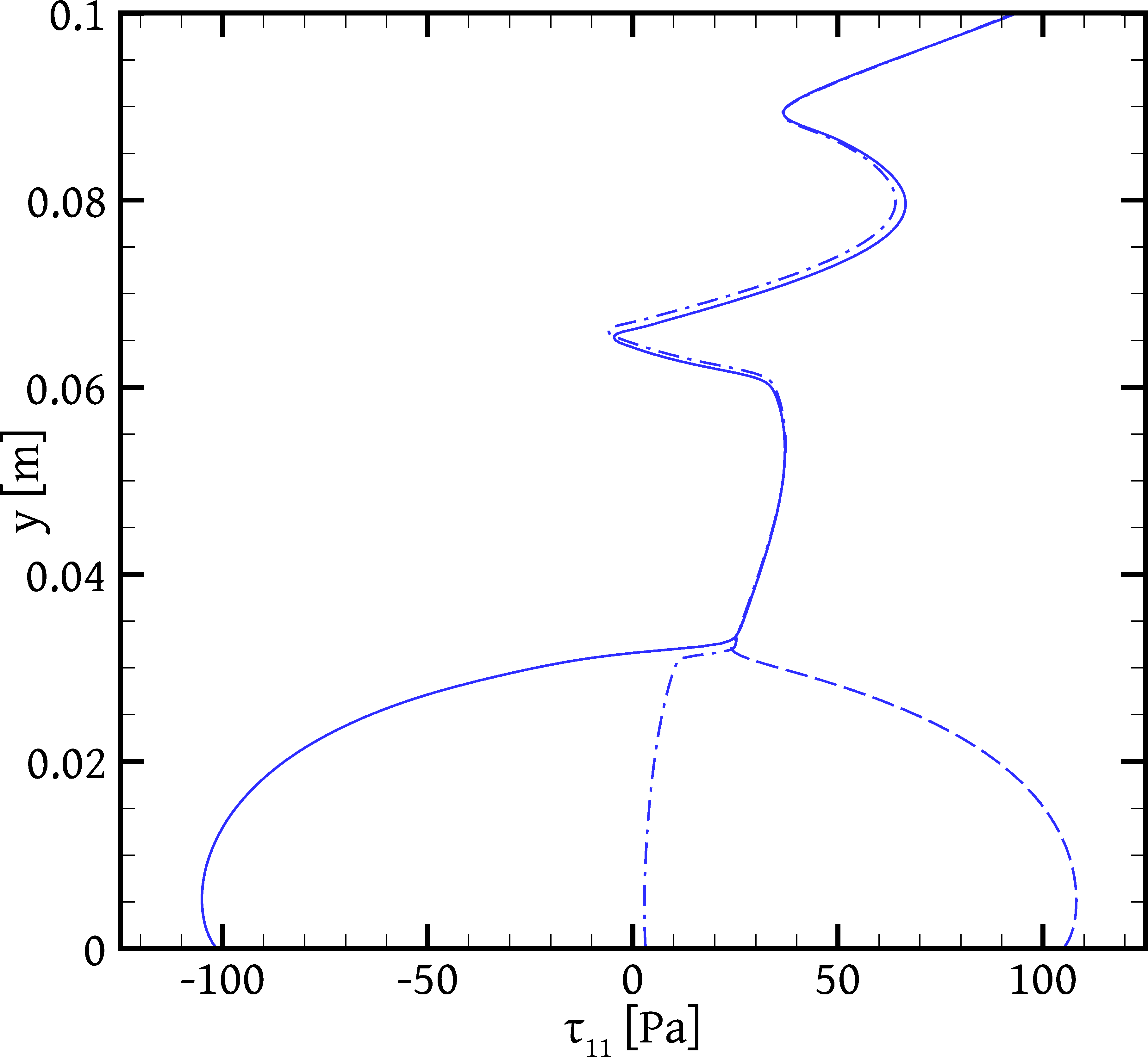
(a) $\tau_{11}$

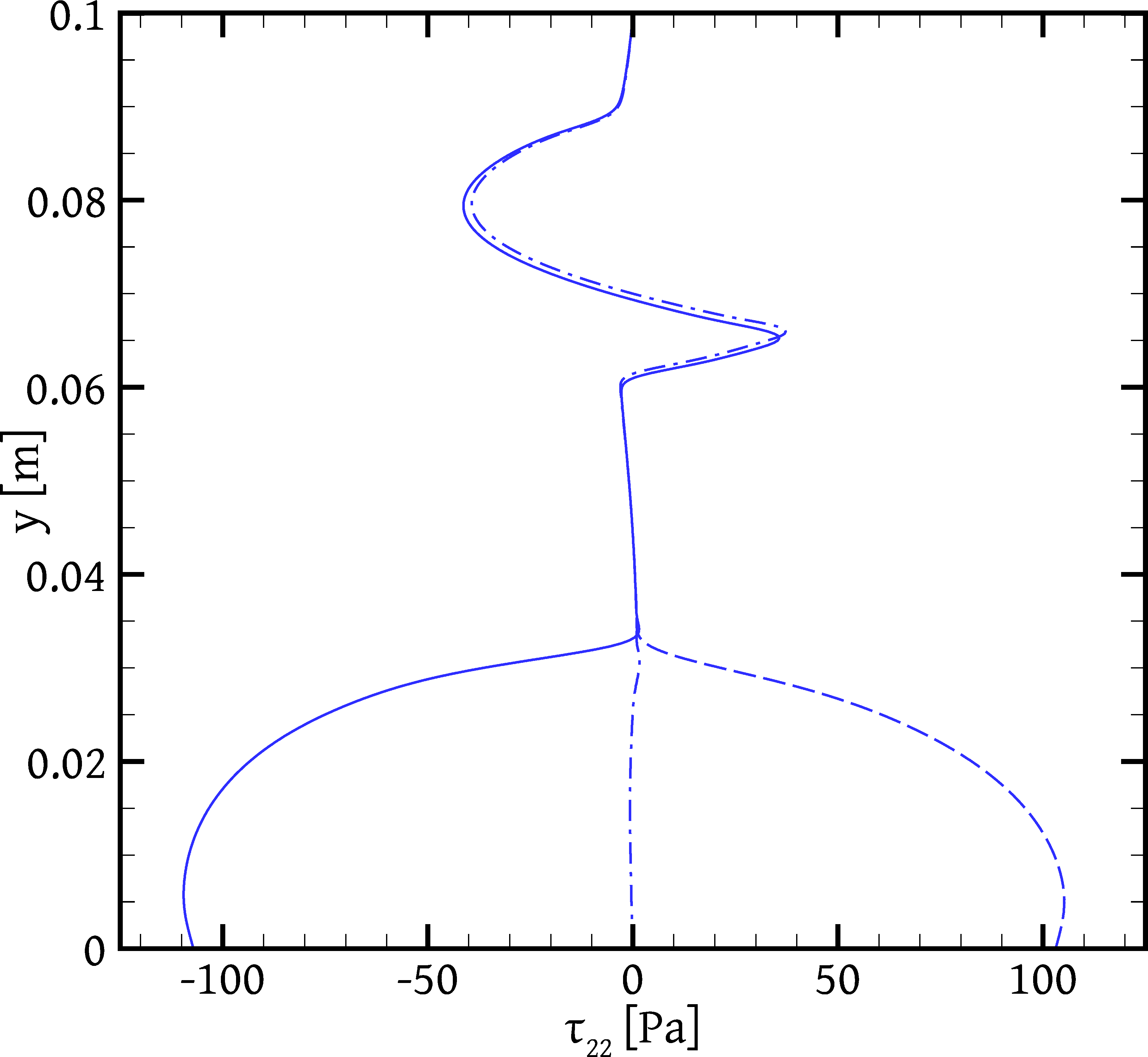
(b) $\tau_{22}$

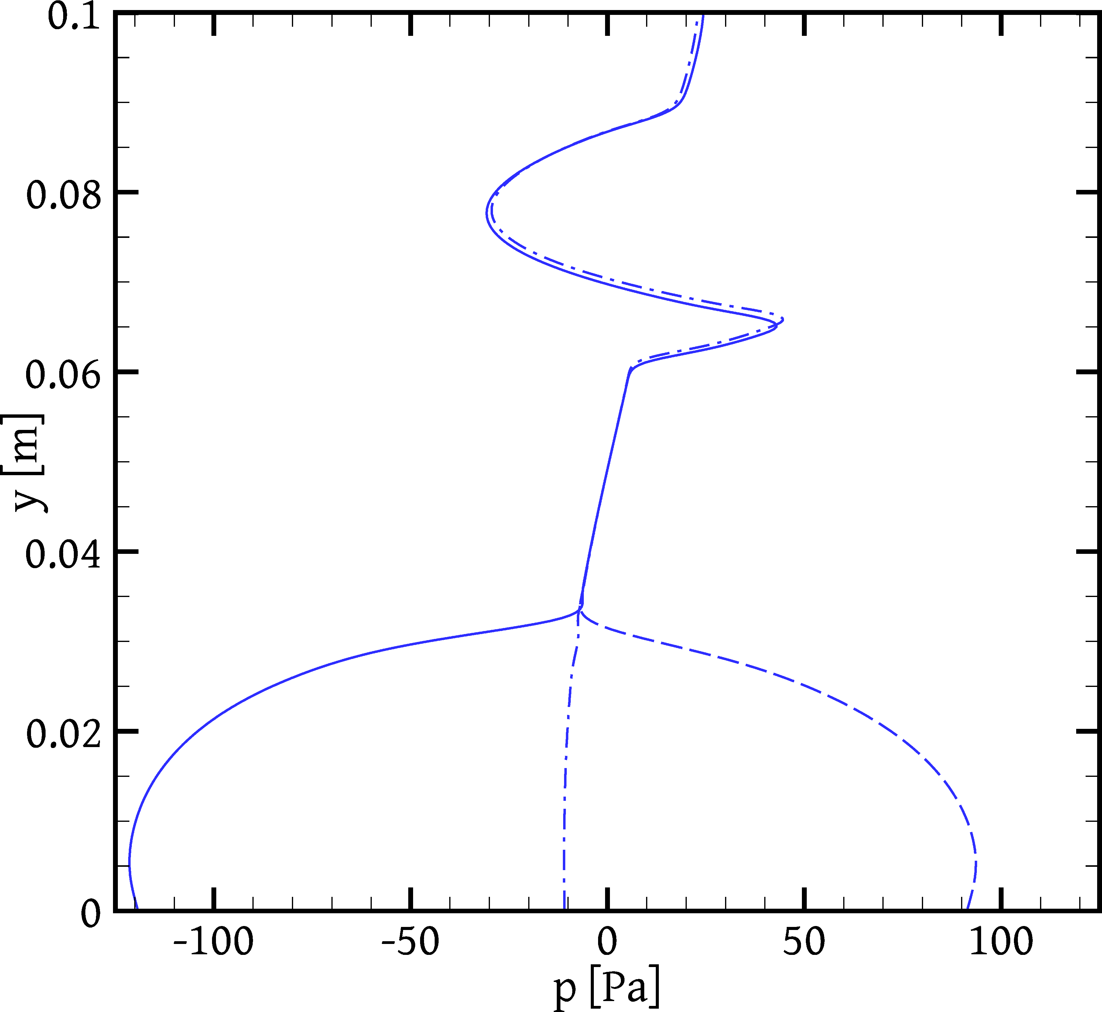
(c) pressure

Figure 23: Normal stress components 23(a)-23(b) and pressure 23(c) along the vertical centreline ($x=L/2$) for the cases with initial conditions $\tau_{11}=\tau_{22}=-\sqrt{3}\tau_{y}$ (continuous lines), $+\sqrt{3}\tau_{y}$ (dashed lines), and zero (dash-dot lines).

6.6 Cessation

Our final investigation concerns the sudden stopping of the lid and the study of the subsequent flow decay. Classic viscoplastic models are known to predict flow cessation in finite time after the driving agent is removed [84]. This can be proved rigorously using variational inequalities (e.g. upper bounds for the cessation times of some one-dimensional flows are derived in [85, 86, 87]), but roughly speaking it is due to the effect of the yield stress on the rate of energy dissipation: it keeps it high enough during the flow decay such that all of the fluid’s kinetic energy (KE) is dissipated in finite time – a rough explanation is sketched in Appendix C. The cessation of viscoplastic (Bingham) lid-driven cavity flow was studied in [40], according to the findings of which we would expect HB flow to cease completely at some time $t_{c}\ll T_{c}\equiv\rho UL/S\approx$ 0.11 $\mathrm{s}$ ($T_{c}$ is the time needed for a force of magnitude $SL^{2}$ to bring a mass of momentum $\rho UL^{3}$ to rest).

The situation concerning SHB flow is expected to be somewhat different. Firstly, even though the energy conversion rate $\int_{\Omega}\underline{\underline{\tau}}\!:\!\nabla\underline{u}\>\mathrm{d}\Omega$ is still expected to be large enough to convert all the KE of the material in finite time, this rate now includes not only energy dissipation, but also energy storage in the form of elastic (potential) energy, which can later be converted back into KE [88]. In fact, once all of the material becomes unyielded there is no mechanism for energy dissipation and it is expected that the remaining energy will perpetually change form from elastic to kinetic and vice versa, resulting in oscillatory motions. Furthermore, the formation of transition regions in previous simulations makes it uncertain whether all of the material will become unyielded in finite time. To investigate these issues, using the “steady-state” base flow (Sec. 6.1) as initial condition, we suddenly stopped the lid motion and carried out a simulation to see how the flow evolves. We repeated the procedure also with the slip case of Sec. 6.4. Figure 24(a) shows the evolution of the KE with time ($t$ = 0 is the instant the lid is halted). In neither case does the flow cease in finite time.

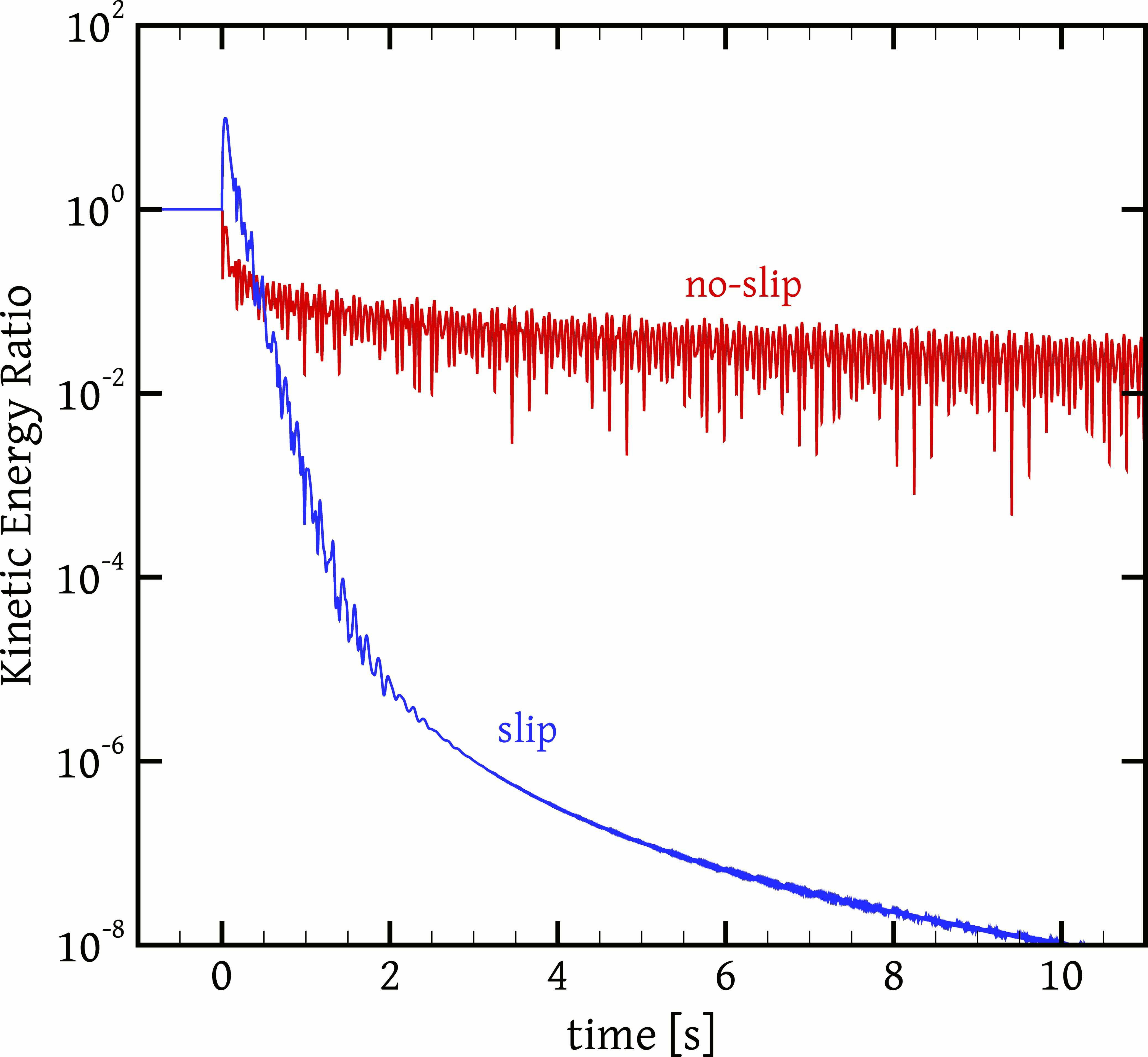
(a)

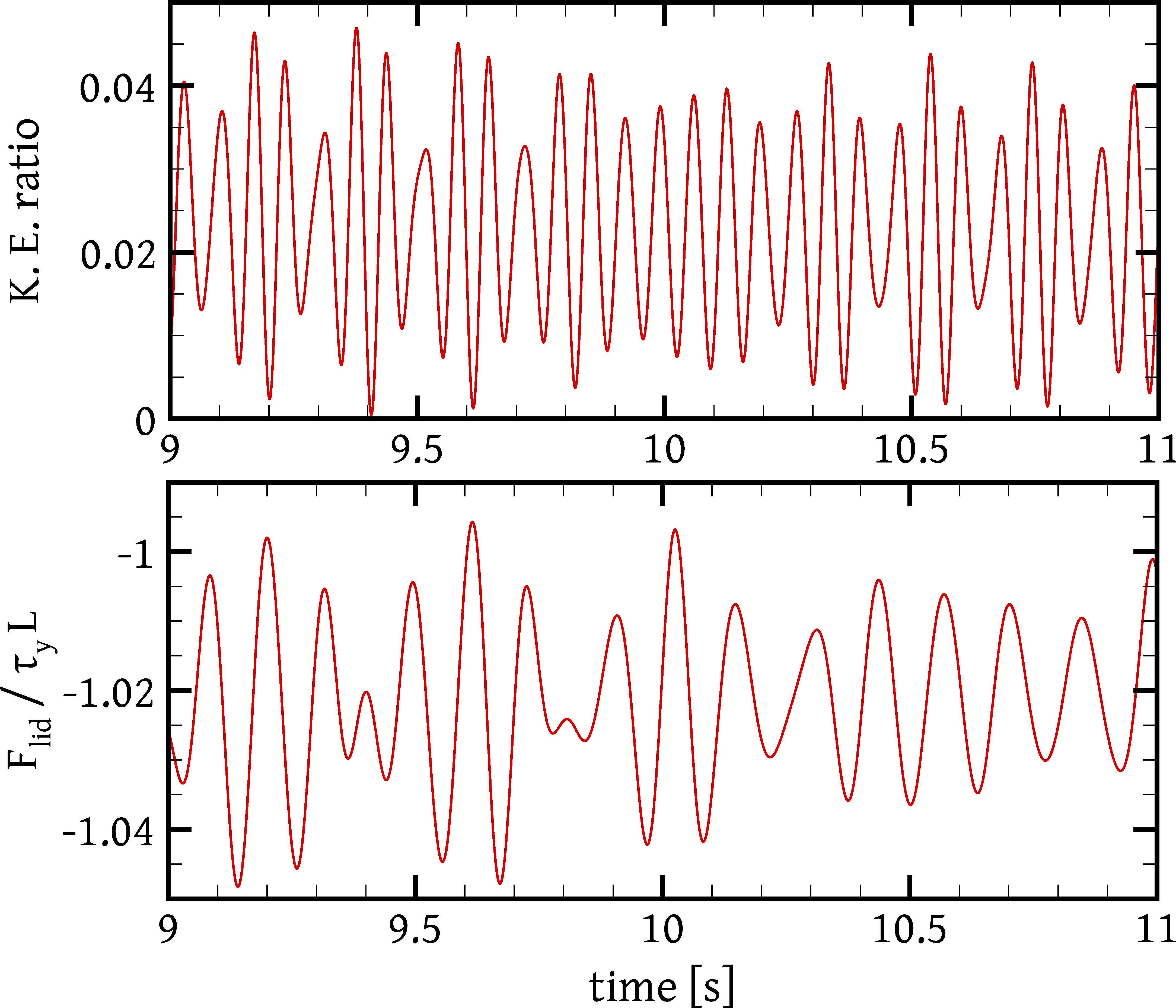
(b)

Figure 24: 24(a): Fluid kinetic energy (Eq. (69)), normalised by its value at the instant the lid is halted, versus time elapsed (the lid is halted at time $t$ = 0) for the no-slip and slip cases. 24(b): The top diagram is a close-up view of a portion of the no-slip curve in 24(a). The bottom diagram plots the corresponding values of the force exerted by the fluid on the lid, normalised by $\tau_{y}L$.

In the no-slip case, the KE history is highly oscillatory, confirming the anticipated perpetual back-and-forth conversion between kinetic and elastic energies. The top diagram of Fig. 24(b) shows a clearer picture over a narrower time window. The KE peaks 29 times within that 2 $\mathrm{s}$ window, i.e. a single oscillation lasts about 69 $\mathrm{m}\mathrm{s}$; the time step is kept to about $\Delta t$ = $2\text{\times}{10}^{-4}$ $\mathrm{s}$ by the adjustable time step scheme, so each KE oscillation period is resolved into about 350 time steps. The diagram shows that the KE variation does not consist of a single harmonic component, and Fig. 25 shows that the flow is indeed quite complex. Usually at any given instant there appears one main vortex rotating in either the clockwise or anticlockwise sense, but its location and shape are not fixed, while smaller vortices may also appear. The material is not completely unyielded, and the yielded zones are transported along as the material oscillates while their size varies with time. The existence of these yielded zones allows some energy dissipation, and hence the mean KE in Fig. 24 very slowly drops. The bottom diagram of Fig. 24(b) shows the force $F_{\mathrm{lid}}$ exerted by the fluid on the lid. This force is negative, pushing the lid towards the left, i.e. in the opposite direction than it was moving prior to its halting. The magnitude of the force oscillates slightly above the value $\tau_{y}L$, and an inspection shows that this is because the magnitude of $\tau_{12}$ on the lid slowly drops towards $\tau_{y}$ (the lid is in touch with a transition zone). Figure 25(i) shows that the magnitude of $F_{\mathrm{lid}}$ drops when the lid touches a clockwise vortex (Figs. 25(b), 25(d), 25(g)) and it increases when it touches a counter-clockwise vortex (Figs. 25(c), 25(e)). A comparison between the KE and $F_{\mathrm{lid}}$ diagrams in Fig. 24(b) shows that $F_{\mathrm{lid}}$ oscillates at a frequency that is roughly half of that of the KE, which is expected since during a single $F_{\mathrm{lid}}$ period both the clockwise and anticlockwise vortex velocities are maximised, which leads to two KE peaks.

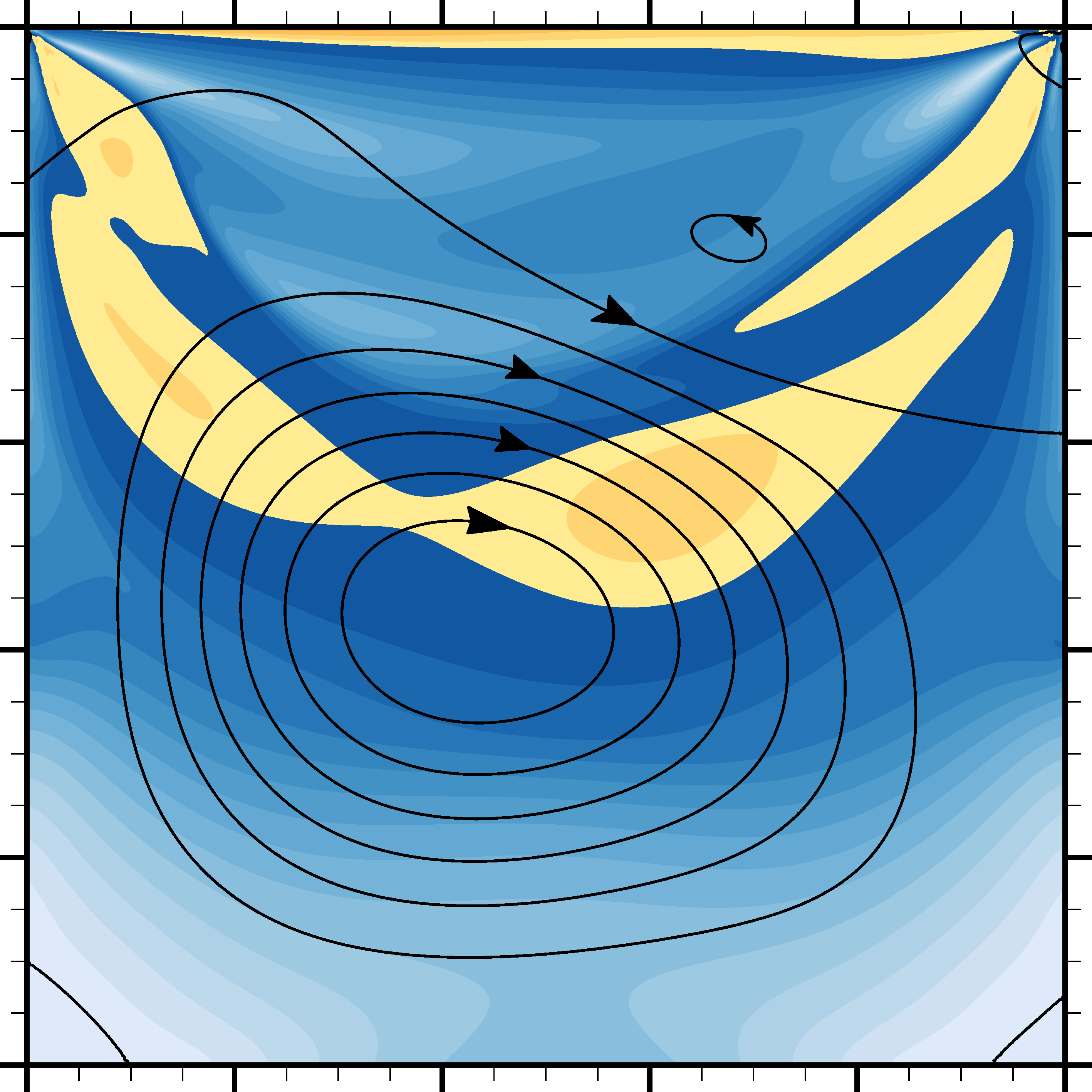
(a) $t$ = 3 $\mathrm{s}$

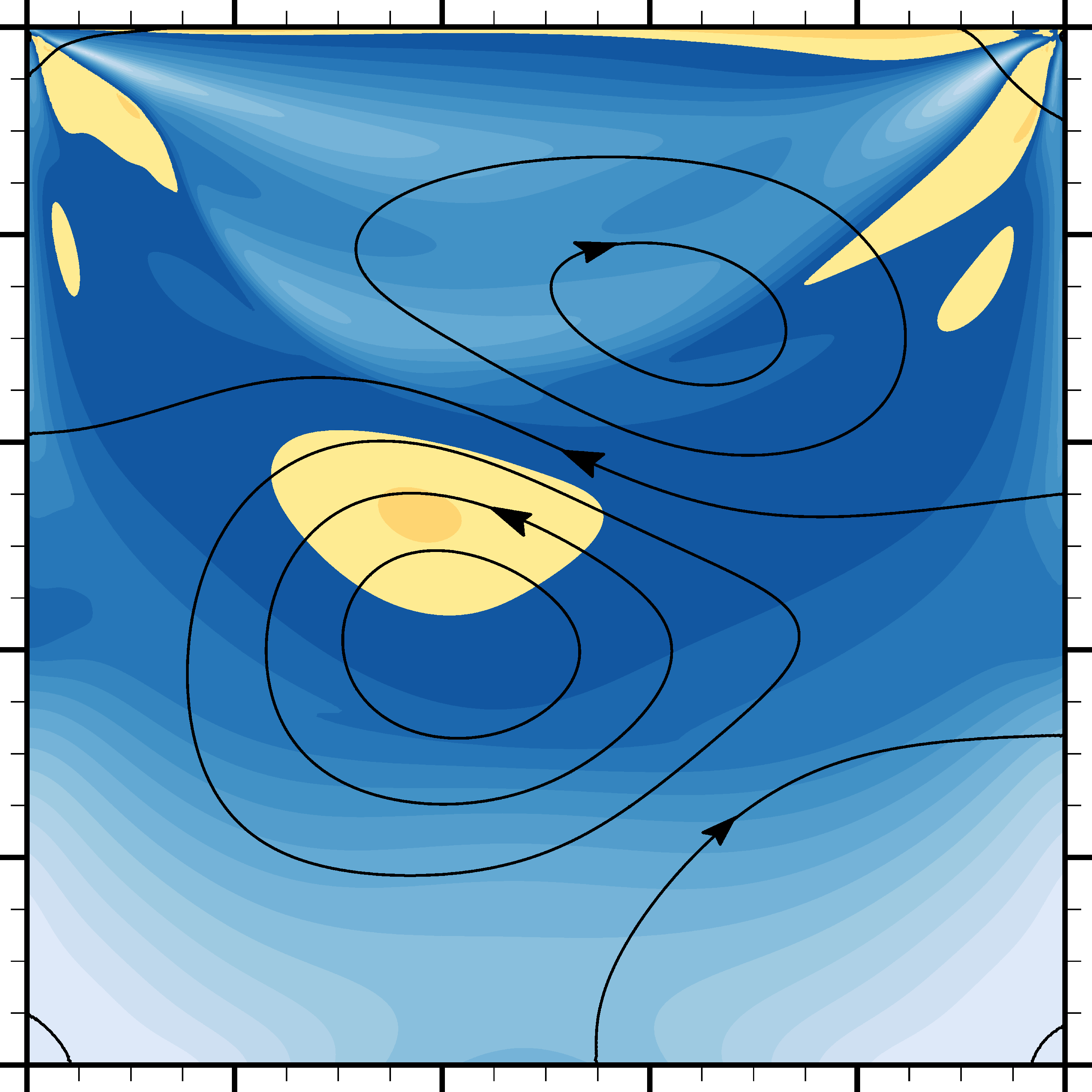
(b) $t$ = 3.05 $\mathrm{s}$

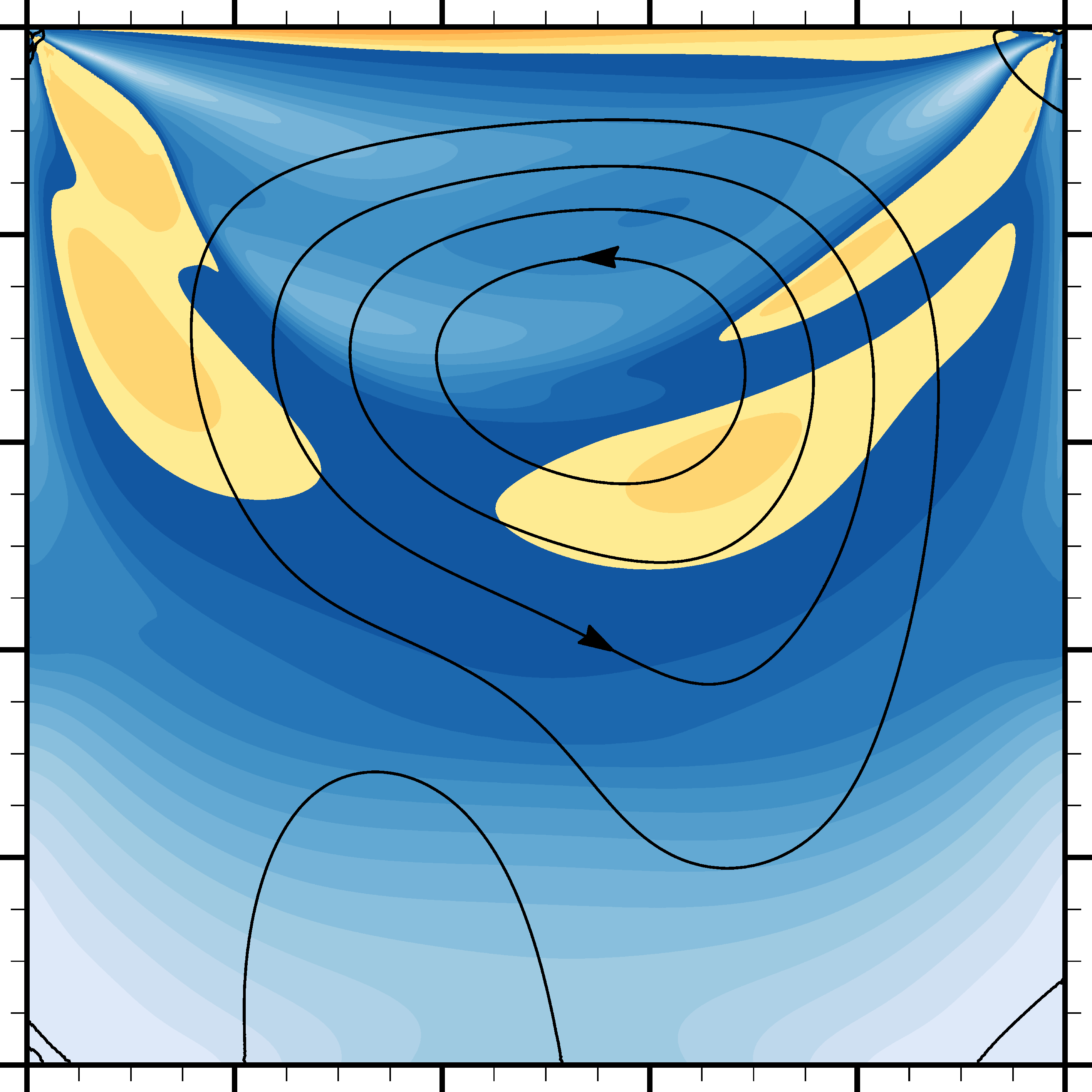
(c) $t$ = 3.10 $\mathrm{s}$

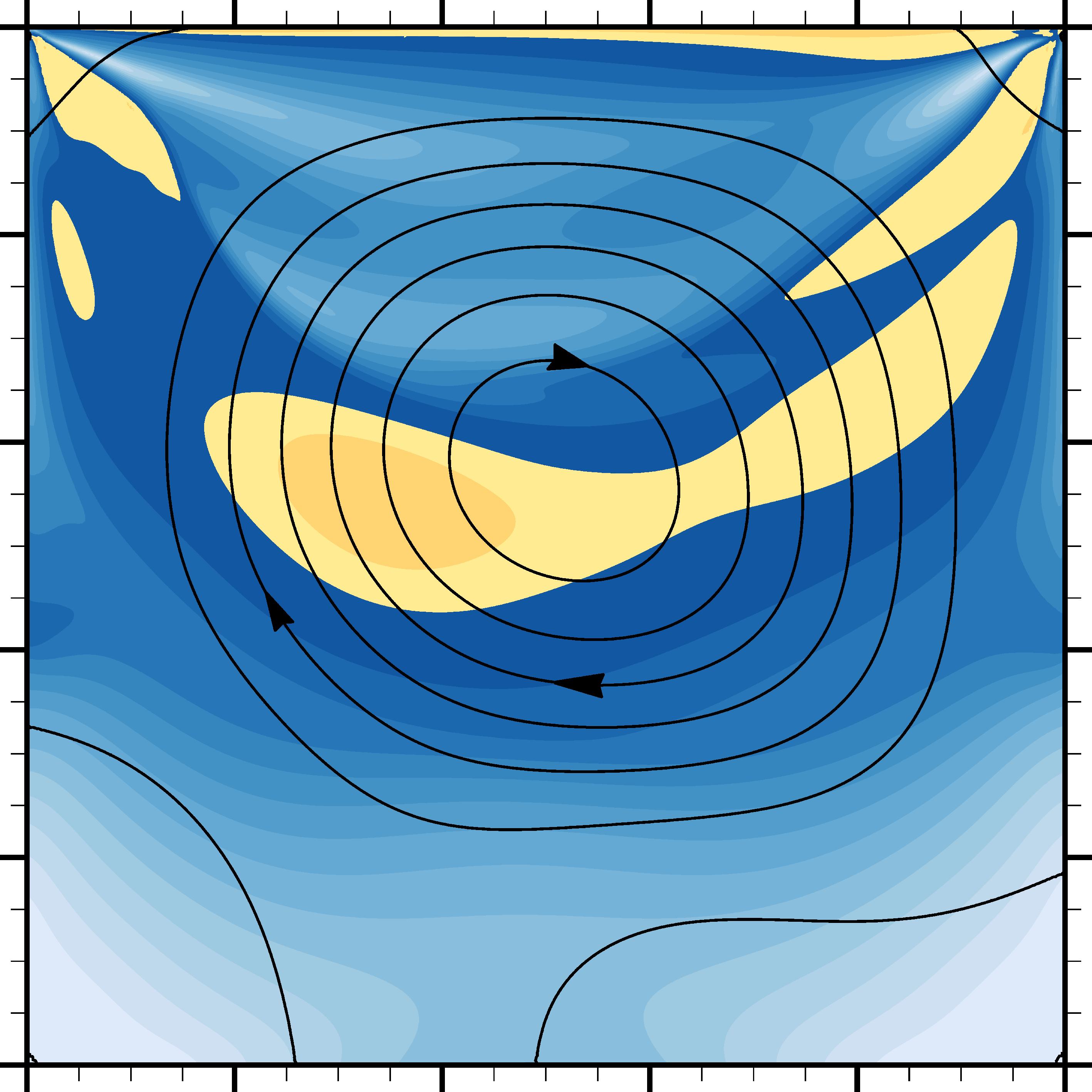
(d) $t$ = 3.15 $\mathrm{s}$

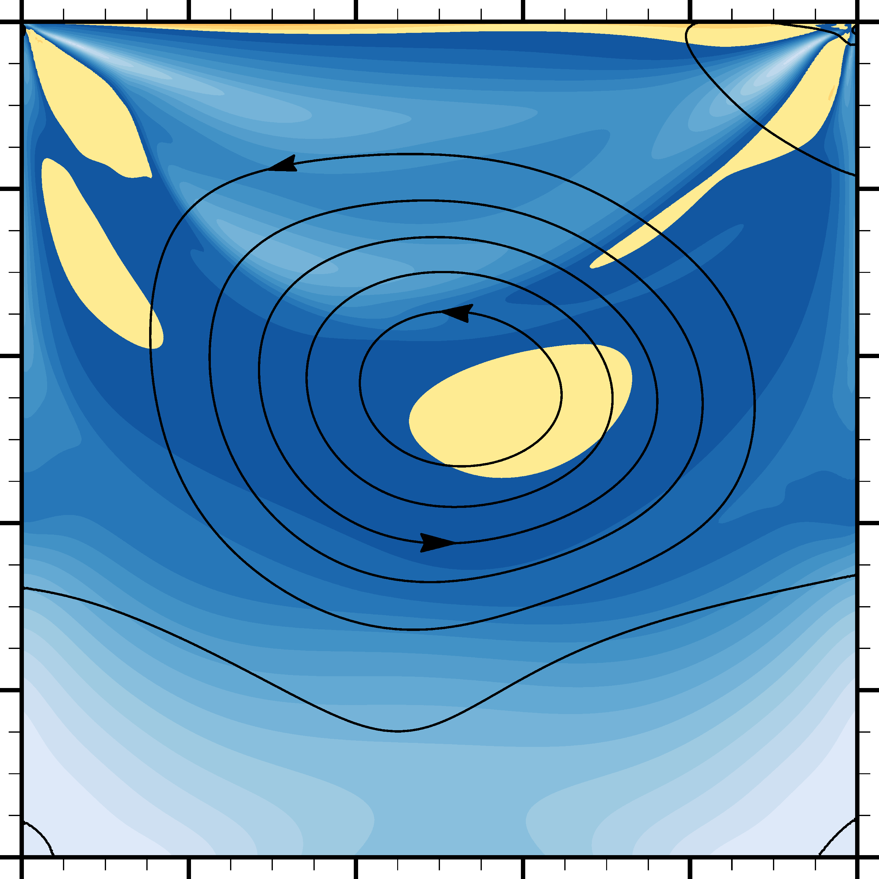
(e) $t$ = 3.20 $\mathrm{s}$

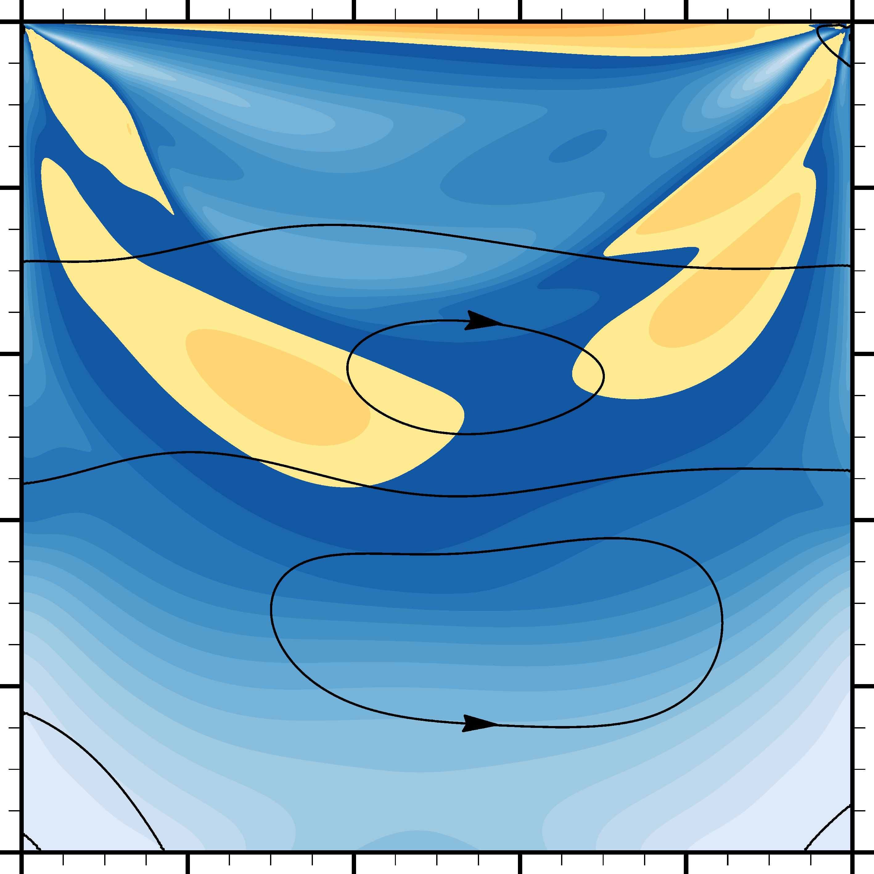
(f) $t$ = 3.25 $\mathrm{s}$

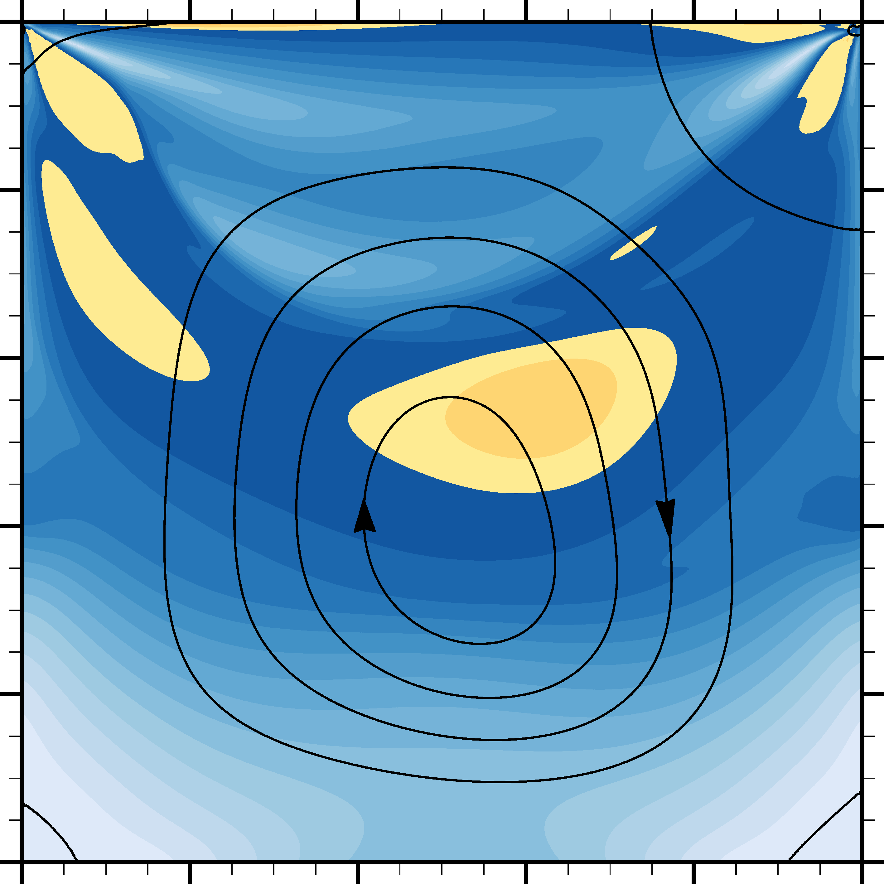
(g) $t$ = 3.30 $\mathrm{s}$

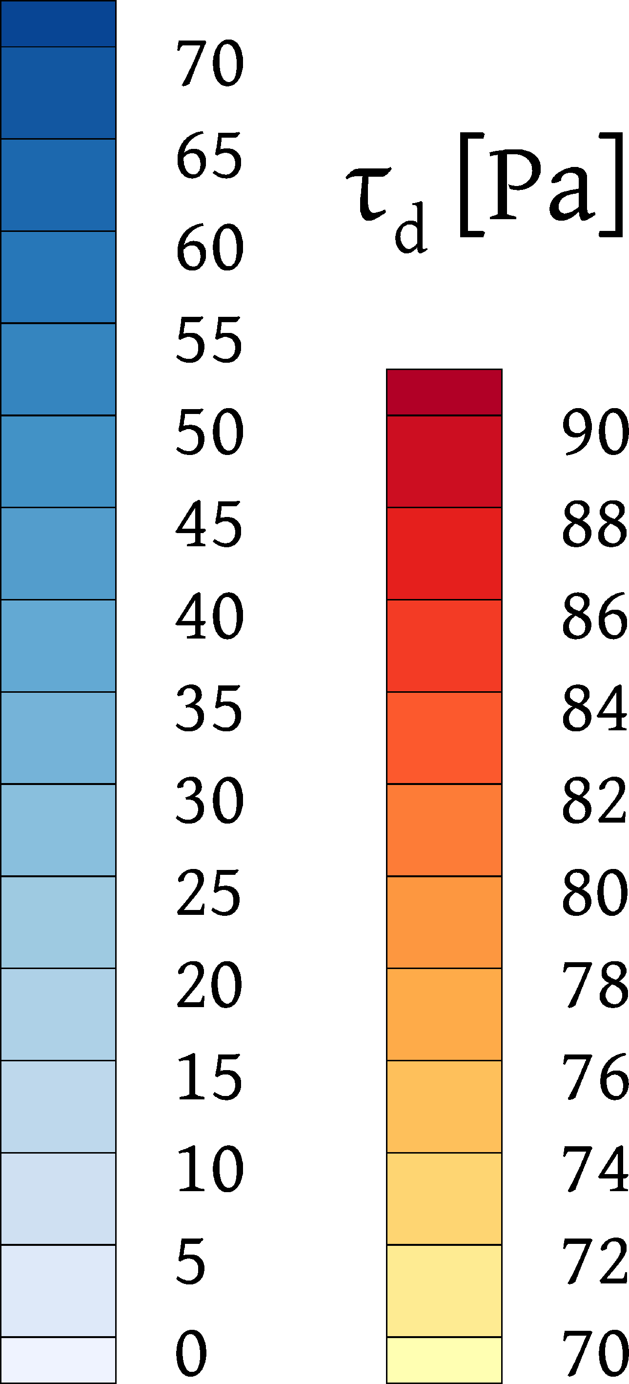
(h) colour map

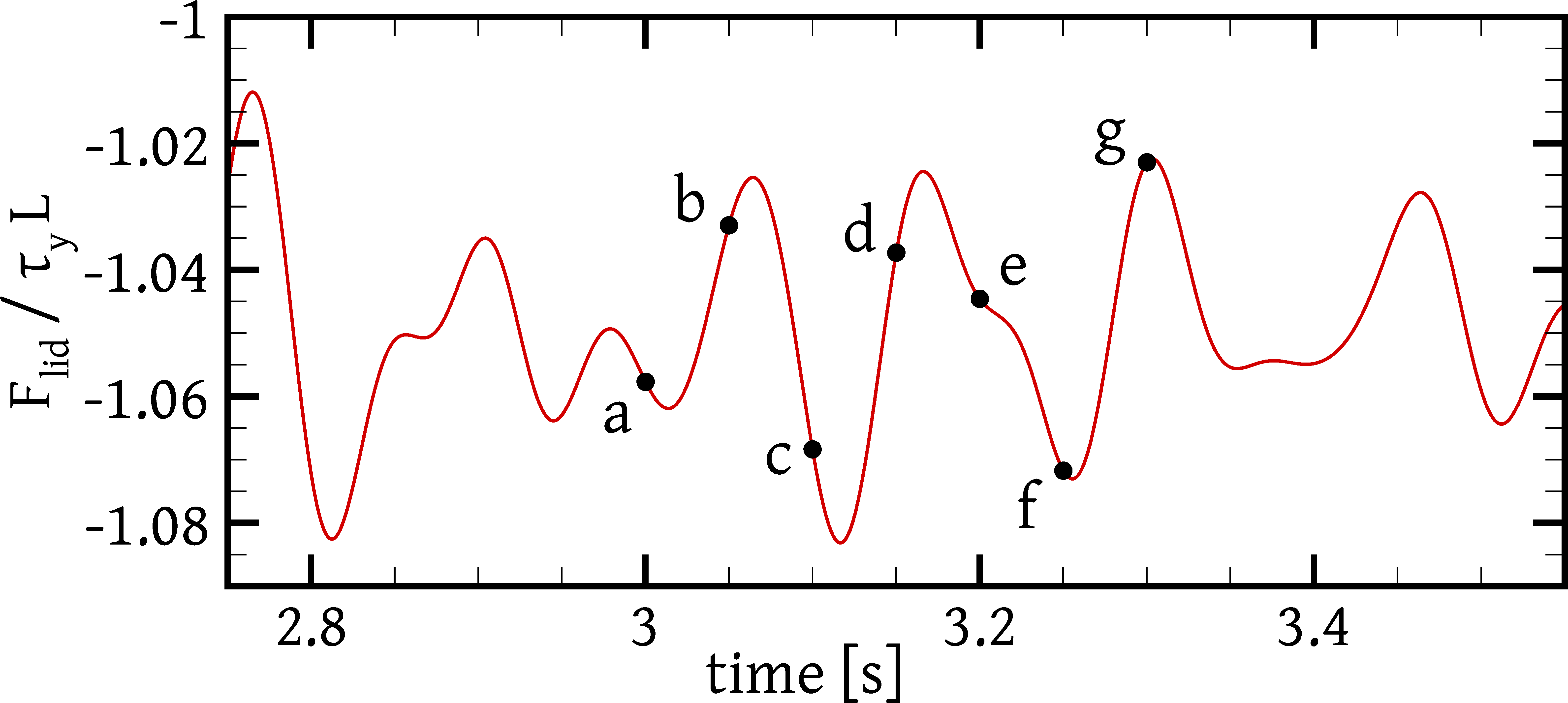
(i) History of $F_{\text{lid}}$

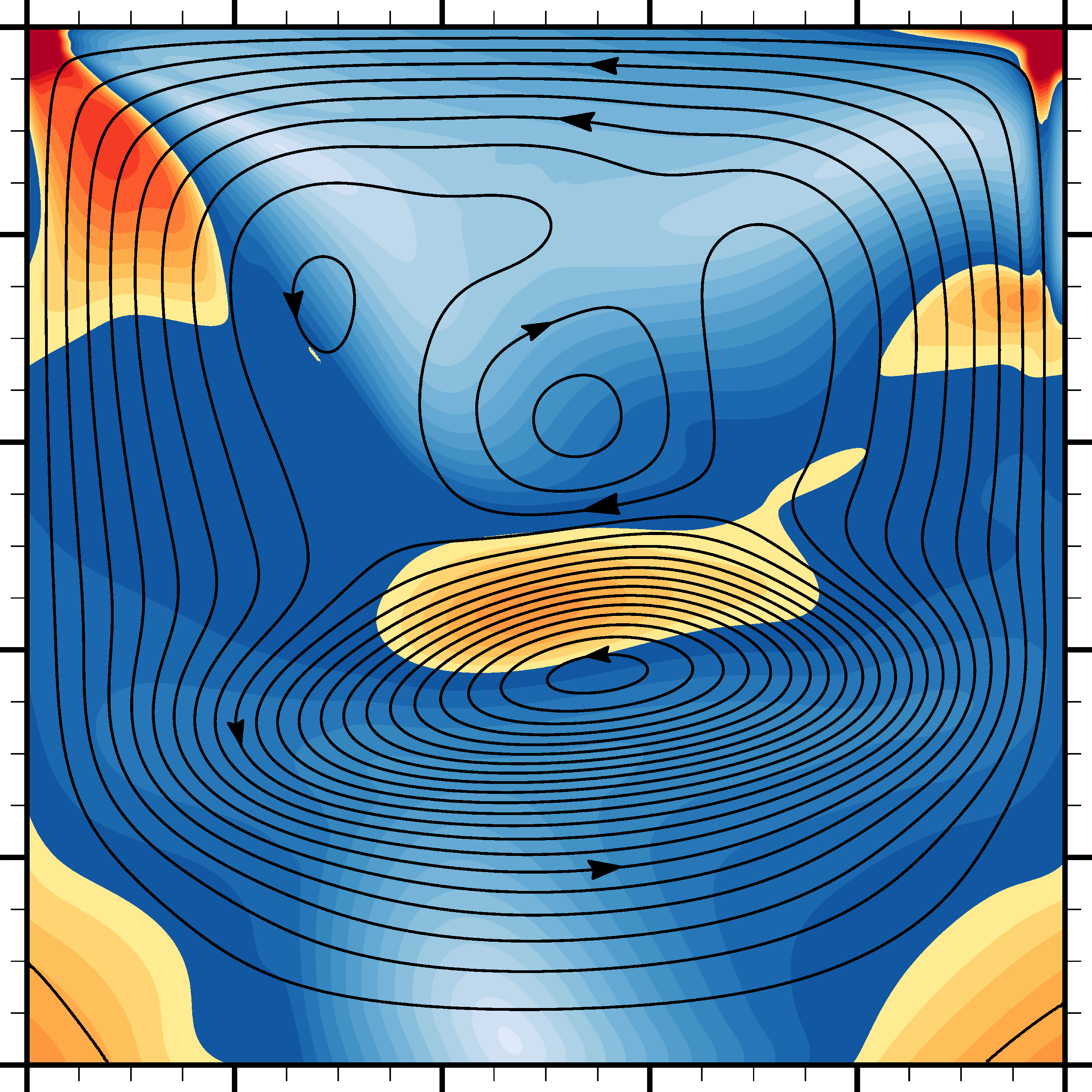
(j) (slip) $t$ = 0.10 $\mathrm{s}$

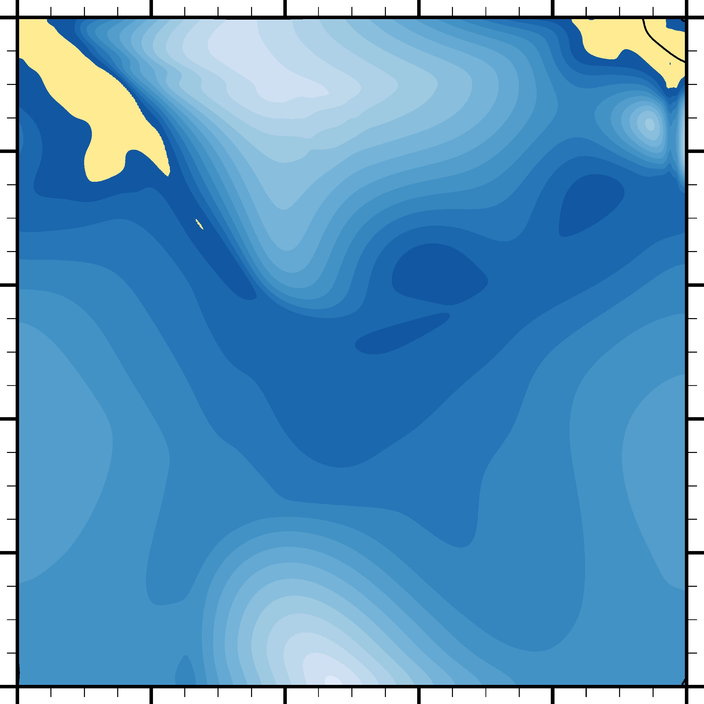
(k) (slip) $t$ = 60 $\mathrm{s}$

Figure 25: 25(a)-25(g): Snapshots of the no-slip cessation flow field, with colour contours of $\tau_{d}$, of different base colour for yielded (yellow) and unyielded (blue) regions (see the colour map 25(h)), and instantaneous streamlines plotted at streamfunction intervals of $\delta\psi/LU=0.002$, with $\psi=0$ as one of the contours. 25(i): Part of the history of the force exerted by the fluid on the lid, normalised by $\tau_{y}L$, with the instants corresponding to snapshots 25(a)-25(g) marked on the plot. 25(j)-25(k): Snapshots of the slip cessation flow field.

In the slip case, the KE peaks immediately after the lid halt (Fig. 24(a)) but then the oscillations die out relatively quickly and the KE diminishes. The KE peak is due to the material recoiling right after the lid halts (Fig. 25(j)), which is possible as the walls provide limited resistance, due to slip. Then, the KE is dissipated through a mechanism that is absent in the no-slip case: as the material oscillates inside the cavity, it slides past the walls due to slip, and the friction at the wall / material interface dissipates the KE. Even in this case, however, transition zones exist long after the lid has halted (Fig. 25(k)).

7 Conclusions

This work presented a FVM for elastoviscoplastic flows described by the SHB model. The method is applicable to collocated structured and unstructured meshes; it incorporates a new variant of momentum interpolation, a variant of “two sides diffusion”, and the CUBISTA scheme, in order to suppress spurious pressure, velocity, and stress oscillations, respectively. The method was shown to achieve this goal, and also to be consistent on both smooth and irregular meshes. Similar stabilisation techniques have recently been applied in a Finite Element context to allow use of equal-order polynomial basis functions for all variables [89]. An implicit temporal discretisation with adaptive time step is employed.

The method was applied to the simulation of EVP flow in a lid-driven cavity, with the SHB parameters chosen so as to represent Carbopol. The results can serve as benchmark solutions, but furthermore the simulations were designed so as to allow investigation of several aspects of the SHB model behaviour. Complementary simulations with the classic HB model were also performed for comparison. It was noticed that the SHB model can predict “transition zones”, regions where the velocity is near-zero and it takes a very long, or infinite, time to transition from a formally yielded to an unyielded state. The differences between the SHB and HB velocity fields are rather small for the lid velocities tested, although some elastic effects are noticeable in the SHB case, such as a slight upstream displacement of the vortex, a downstream stretching of the plug zone, and a small swelling of the bottom unyielded zone, compared to the HB results. These differences diminish by increasing the elastic modulus $G$, although the convergence of the SHB and HB yield lines is rather slow and requires very large values of $G$. The velocity fields converge much faster. We also applied slip at the walls, as EVP materials are slippery, in which case no transition zones developed.

Motivated by the observation of Cheddadi et al. [32] that different initial conditions of stress can lead to different steady states even as concerns the velocity, we performed two additional simulations where the initial state of the material was stationary but on the verge of yielding, with either compressive or tensile residual stresses, respectively. Indeed, although both of these simulations converged to the same steady-state velocity field, that field was slightly but noticeably different than that obtained when the initial stresses were zero. Due to this property of the SHB model, an accurate calculation of a steady state requires not only sufficient spatial resolution (grid spacing) but also sufficient temporal resolution (time step size), which is facilitated by the use of an adaptive time discretisation scheme such as the one proposed herein.

Finally, simulations of the cessation of the flow after the lid is suddenly halted were performed, which showed that, unlike what is predicted by the HB model, the flow does not cease in finite time but there is a perpetual back-and-forth conversion between kinetic and elastic energies. In the no-slip case, a very slow net energy dissipation was observed, which is possible due to the persisting existence of yielded regions. The energy dissipation is much faster under wall slip, due to friction between the material and the walls.

Incorporation of additional rheological phenomena such as thixotropy is planned for the future.

Appendix A The SHB extra stress tensor in the limit of infinite elastic modulus

The SHB constitutive equation (7) distinguishes between $\underline{\underline{\tau}}$ and $\underline{\underline{\tau}}{}_{d}$, unlike the HB equation (4). For the two models to become equivalent as $G\rightarrow\infty$ it is necessary that $\underline{\underline{\tau}}\rightarrow\underline{\underline{\tau}}{}_{d}$ or, equivalently, $\mathrm{tr}(\underline{\underline{\tau}})\rightarrow 0$.

In the limiting case $G\rightarrow\infty$ the first term on the left-hand side of Eq. (7) diminishes. This makes yielded material (where the “max” term is non-zero) tend to behave as a generalised Newtonian fluid so that $\mathrm{tr}(\underline{\underline{\tau}})\rightarrow 0\Rightarrow\underline{\underline{\tau}}\rightarrow\underline{\underline{\tau}}{}_{d}$ and the two models do become equivalent in yielded regions. On the other hand, in unyielded regions (where the “max” term is zero) Eq. (7) tends to reduce to $\dot{\underline{\underline{\gamma}}}=0$, which does not, at first glance, imply that $\underline{\underline{\tau}}\rightarrow\underline{\underline{\tau}}{}_{d}$. However, the following observation can be made. In an unyielded region the SHB model can be written as (substituting Eq. (8) into Eq. (7))

$$\frac{D\underline{\underline{\tau}}}{Dt}\;\equiv\;\frac{\partial\underline{\underline{\tau}}}{\partial t}\;+\;\underline{u}\cdot\nabla\underline{\underline{\tau}}\;=\;G\dot{\underline{\underline{\gamma}}}\;+\;G\left((\nabla\underline{u})^{\mathrm{T}}\cdot\underline{\underline{\tau}}\;+\;\underline{\underline{\tau}}\cdot\nabla\underline{u}\right)$$ (A.1)

The material derivative $D\underline{\underline{\tau}}/Dt$ is the rate of change of the stress tensor with respect to time in a fluid particle moving with the flow. This derivative is applied component-wise to the stress tensor, and therefore the rate of change of $\mathrm{tr}(\underline{\underline{\tau}})$ is

$$\frac{D(\mathrm{tr}(\underline{\underline{\tau}}))}{Dt}\;=\;\mathrm{tr}\left(\frac{D\underline{\underline{\tau}}}{Dt}\right)$$ (A.2)

or, using Eq. (A.1),

$$\frac{D(\mathrm{tr}(\underline{\underline{\tau}}))}{Dt}\;=\;G\>\mathrm{tr}(\dot{\underline{\underline{\gamma}}})\;+\;G\>\mathrm{tr}\left((\nabla\underline{u})^{\mathrm{T}}\cdot\underline{\underline{\tau}}\;+\;\underline{\underline{\tau}}\cdot\nabla\underline{u}\right)$$ (A.3)

In the right-hand side, $\mathrm{tr}(\dot{\underline{\underline{\gamma}}})\rightarrow 0$ because in the unyielded regions $G\rightarrow\infty$ forces $\dot{\underline{\underline{\gamma}}}\rightarrow 0$. For the second term in the right-hand side, in index notation, we have

$$(\nabla\underline{u})^{\mathrm{T}}\cdot\underline{\underline{\tau}}\;+\;\underline{\underline{\tau}}\cdot\nabla\underline{u}\;=\;\sum_{i=1}^{3}\sum_{j=1}^{3}\left(\sum_{k=1}^{3}\frac{\partial u_{i}}{\partial x_{k}}\tau_{kj}\;+\;\sum_{k=1}^{3}\frac{\partial u_{j}}{\partial x_{k}}\tau_{ik}\right)\underline{e}_{i}\underline{e}_{j}$$ (A.4)

where $\underline{e}_{i}$ is the unit vector in the direction $i$. Taking the trace of the above expression we obtain

$$\mathrm{tr}\left((\nabla\underline{u})^{\mathrm{T}}\cdot\underline{\underline{\tau}}\;+\;\underline{\underline{\tau}}\cdot\nabla\underline{u}\right)\;=\;\sum_{i=1}^{3}\sum_{j=1}^{3}\left(\frac{\partial u_{j}}{\partial x_{i}}\,+\,\frac{\partial u_{i}}{\partial x_{j}}\right)\tau_{ij}$$ (A.5)

The terms in parentheses in the sum (A.5) are just the components of $\dot{\underline{\underline{\gamma}}}$, and so they tend to zero as $G\rightarrow\infty$. Thus the whole right-hand side of Eq. (A.3) tends to zero in the unyielded regions as $G\rightarrow\infty$. Therefore, under these conditions, $D(\mathrm{tr}(\underline{\underline{\tau}}))/Dt\rightarrow 0$, i.e. $\mathrm{tr}(\underline{\underline{\tau}})$ remains constant in any particle moving in an unyielded region. Given that $\mathrm{tr}(\underline{\underline{\tau}})=0$ for yielded particles, as mentioned above, there appears to be no mechanism for $\mathrm{tr}(\underline{\underline{\tau}})$ to acquire any value different than zero. Thus we expect that $\underline{\underline{\tau}}\rightarrow\underline{\underline{\tau}}{}_{d}$ also in the unyielded regions. But even if $\mathrm{tr}(\underline{\underline{\tau}})\neq 0\Rightarrow\underline{\underline{\tau}}\neq\underline{\underline{\tau}}{}_{d}$ in such a region, for practical purposes the stress field would still be equivalent to a HB stress field where the isotropic part of $\underline{\underline{\tau}}$ is incorporated into the pressure.

Appendix B Effect of grid refinement on the pressure stabilisation scheme

It follows from the definition of $a_{f}^{mi}$ (33) that as the grid is refined ($h_{f}\rightarrow 0$) the viscous term in the denominator dominates over the inertial one: at fine grids $a_{f}^{mi}\approx h_{f}/(2\kappa+2\eta_{a})$. This can be explained with the aid of the simple one-dimensional example used for deriving the scheme. From Eq. (38), if we want to locally perturb a velocity field at point $c$ by $u^{\prime}_{c}$ (Fig. 26) by locally perturbing the pressure gradient by $-\mathrm{d}p^{\prime}/\mathrm{d}x|_{c}\approx(p^{\prime}_{P}-p^{\prime}_{N})/h$ then these perturbations are related by

$$u^{\prime}_{c}\;=\;\frac{1}{\rho\left(\left.\dfrac{\mathrm{d}u}{\mathrm{d}x}\right|_{c}\>+\;\dfrac{1}{\Delta t}\right)\;+\;\dfrac{2\eta_{c}}{h^{2}}}\;\cdot\;\frac{p^{\prime}_{P}-p^{\prime}_{N}}{h}\;=\;O(h^{2})\cdot\left.\frac{\mathrm{d}p^{\prime}}{\mathrm{d}x}\right|_{c}\;\;\Rightarrow\;\;\left.\frac{\mathrm{d}p^{\prime}}{\mathrm{d}x}\right|_{c}\;=\;O(h^{-2})\cdot u^{\prime}_{c}$$ (B.1)

Thus, in order to effect a local velocity perturbation of wavelength equal to the grid spacing, as shown in Fig. 26, the pressure gradient must be adjusted locally by an amount that scales as $(h^{-2})$, i.e. it must become larger and larger as the grid is refined. This is because it has to overcome the viscous resistance which scales as $\mathrm{d}^{2}u^{\prime}/\mathrm{d}x^{2}|_{c}=O(h^{-2})$: grid refinement not only increases the velocity slopes (and associated viscous stresses) but also changes these slopes over a shorter distance (Fig. 26). On the contrary, the part of the pressure gradient that is needed to balance the inertial contribution of $u^{\prime}_{c}$ to the momentum balance is independent of the grid spacing. Conversely, Eq. (B.1) shows that fixed localised perturbations of the pressure gradient of wavelength equal to the grid spacing cause local velocity perturbations of magnitude $O(h^{2})$, which become smaller and smaller with grid refinement due to increased viscous resistance.

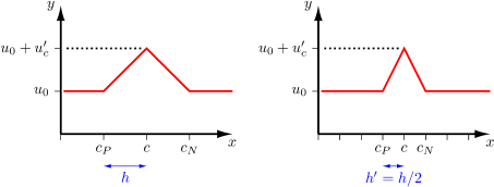
Figure 26: A local velocity perturbation $u^{\prime}_{c}$ with wavelength equal to the grid spacing $h$ causes local perturbations $\mathrm{d}u^{\prime}/\mathrm{d}x$ to the velocity gradient that are proportional to $u^{\prime}_{c}/h=O(h^{-1})$; it follows that the corresponding perturbations to the second derivative of velocity $\mathrm{d}^{2}u^{\prime}/\mathrm{d}x^{2}$ are proportional to $O(h^{-1})/h=O(h^{-2})$.

The pseudo-velocities $u_{f}^{p+}$ and $u_{f}^{p-}$ defined by Eqs. (31) and (32), have magnitudes of $O(h^{2})$ (because $a_{f}^{mi}=O(h)$ and, in smooth pressure fields, both $p_{P}-p_{N}$ and $\nabla p\cdot(\underline{P}-\underline{N})$ are $O(h)$), whereas the actual velocity $\bar{\underline{u}}{}_{c_{f}}$ in (30) does not diminish with refinement but tends to a finite value, the exact velocity at the given point. Therefore, as the grid is refined the mass flux becomes dominated by the interpolated velocity $\bar{\underline{u}}{}_{c_{f}}$ while the stabilisation pseudo-velocities $u_{f}^{p+}$ and $u_{f}^{p-}$ diminish. This may raise concerns that the stabilising effect of the scheme may also diminish. However, this is not the case. Suppose that spurious pressure oscillations do arise, of amplitude $\Delta p^{o}$ (in the absence of preventive measures, this amplitude is unaffected by grid refinement [42]). The total pressure can be decomposed into a smooth part, which is close to the exact solution, and a spurious oscillatory part: $p=p^{s}+p^{o}$. Then the sum of pseudo-velocities at point $c$ of the grid shown in Fig. 4 is equal to

$$u_{c}^{p+}\;-\;u_{c}^{p-}\; =\;a_{c}^{mi}\left[(p^{s}_{P}+p^{o}_{P})-(p^{s}_{N}+p^{o}_{N})\;-\;\bar{\nabla}^{q}_{h}(p^{s}+p^{o})_{c}\cdot(\underline{P}-\underline{N}{}_{f})\right]$$

$$=\;a_{c}^{mi}\Big{[}\Delta p^{o}\;+\;\underbrace{(p^{s}_{P}-p^{s}_{N})\;-\;\bar{\nabla}^{q}_{h}p^{s}_{c}\cdot(\underline{P}-\underline{N}{}_{f})}_{O(h^{2})\;\mathrm{or}\;O(h^{3})}\Big{]}$$

$$\approx\;a_{c}^{mi}\,\Delta p^{o}$$ (B.2)

because $p^{o}_{P}-p^{o}_{N}=\Delta p^{o}$ and $\nabla^{q}_{h}p^{o}_{P}=\nabla^{q}_{h}p^{o}_{N}=0$ (the $\nabla^{q}_{h}$ operator is insensitive to oscillations). Also, according to the discussion of Eq. (35), the underlined terms add up to $O(h^{2})$ (or $O(h^{3})$ on smooth structured grids), which is small compared to $\Delta p^{o}$. In other words, $u_{f}^{p+}$ cancels out with the smooth part of $u_{f}^{p-}$ but leaves out the oscillatory part. A similar consideration for point $c_{P}$ (Fig. 4) leads to

$$u_{c_{P}}^{p+}\;-\;u_{c_{P}}^{p-}\;\approx\;-a_{c_{P}}^{mi}\,\Delta p^{o}$$ (B.3)

where the minus sign comes from the fact that, according to the nature of the spurious oscillation, if the oscillatory pressure component decreases by $\Delta p^{o}$ from $P$ to $N$, then it increases by $\Delta p^{o}$ from $PP$ to $P$. Then the combined contribution of faces $c$ and $c_{P}$ to the image of the continuity operator for cell $P$ (the left-hand side of Eq. (34)) divided by the cell volume is

$$\frac{1}{\Omega_{P}}\left[\dot{M}_{c}+\dot{M}_{c_{P}}\right]\;=\;\frac{1}{h^{2}}\rho\,h\left[(\bar{u}_{c}\>+\>u_{c}^{p+}\>-\>u_{c}^{p-})\;-\;(\bar{u}_{c_{P}}\>+\>u_{c_{P}}^{p+}\>-\>u_{c_{P}}^{p-})\right]$$

which, using Eqs. (B.2) and (B.3), and also assuming that $a_{c}^{mi}\approx a_{c_{P}}^{mi}\approx Ch$ for some constant $C$ ($C=2(\kappa+\eta_{a})$ if the grid is fine enough, from Eq. (33)), becomes

$$\frac{1}{\Omega_{P}}\left[\dot{M}_{c}+\dot{M}_{c_{P}}\right]\;=\;\rho\frac{\bar{u}_{c}-\bar{u}_{c_{P}}}{h}\;+\;2\rho C\Delta p^{o}$$ (B.4)

The first term on the right-hand side is the contribution of the actual velocities to the continuity image, and can be seen to tend to the $h$-independent value $\rho\partial u/\partial x|_{P}$ with grid refinement. The second term on the right-hand side is the contribution of the pseudo-velocities, which can also be seen to be $h$-independent, i.e. it does not diminish with grid refinement, although the pseudo-velocities themselves do diminish compared to the actual velocities, as mentioned above. If we take into account also the other two faces of cell $P$ (the horizontal ones) then the total contribution of the pseudo-velocities to the continuity image is $4\rho C\Delta p^{o}$. If we repeat this analysis for the neighbouring cells $N$ and $PP$, then it will turn out that the contributions of the pseudo-velocities to the continuity images of those cells are $-4\rho C\Delta p^{o}$, i.e. they have opposite sign to that of cell $P$. Overall, in the presence of pressure oscillations the contributions of the pseudo-velocities to the continuity image over the entire grid have a checkerboard (oscillatory) pattern like the one shown in Fig. 3, with amplitude proportional to the amplitude of the pressure oscillations, $\Delta p^{o}$. As discussed in relation to Eq. (24), when solving the system of all continuity equations (34), because the right-hand side is smooth (it is zero), spurious pressure oscillations, which would produce an oscillatory right-hand side, are excluded.

Thus, the effectiveness of momentum interpolation in suppressing spurious pressure oscillations does not degrade with grid refinement. The amplitude of the oscillations produced by momentum interpolation to the continuity image is proportional to the amplitude of the spurious pressure oscillations themselves, and independent of the grid spacing $h$.

Appendix C Energy dissipation and flow cessation

This appendix sketches an explanation for the finite cessation times of HB fluids, but for rigorous proofs the reader is referred to the literature cited in Sec. 6.6. For inelastic fluids, once the lid motion ceases, the rate of energy dissipation equals the rate of decrease of the kinetic energy of the fluid [88].

$$\frac{\mathrm{d}}{\mathrm{d}t}\int_{\Omega}\tfrac{1}{2}\rho\underline{u}\cdot\underline{u}\,\mathrm{d}\Omega\;=\;-\int_{\Omega}\underline{\underline{\tau}}:\nabla\underline{u}\,\mathrm{d}\Omega$$ (C.1)

For generalised Newtonian fluids ($\underline{\underline{\tau}}\;=\;\eta(\dot{\gamma})\,\dot{\underline{\underline{\gamma}}}$) we have

$$\underline{\underline{\tau}}:\nabla\underline{u}\;=\;\eta(\dot{\gamma})\,\dot{\underline{\underline{\gamma}}}:\nabla\underline{u}\;=\;\eta(\dot{\gamma})\,\dot{\gamma}^{2}$$ (C.2)

For a HB fluid, $\eta(\dot{\gamma})=(\tau_{y}+k\dot{\gamma}^{n})/\dot{\gamma}$ and the energy dissipation rate (C.2) becomes $(\tau_{y}+k\dot{\gamma}^{n})\,\dot{\gamma}$; in fact, this expression holds even in unyielded regions as it predicts zero energy dissipation there due to $\dot{\gamma}=0$. So, for HB flow the energy balance (C.1) becomes

$$\frac{\mathrm{d}}{\mathrm{d}t}\int_{\Omega}\tfrac{1}{2}\rho\underline{u}\cdot\underline{u}\,\mathrm{d}\Omega\;=\;-\int_{\Omega}\left(\tau_{y}\,+\,k\dot{\gamma}^{n}\right)\dot{\gamma}\,\mathrm{d}\Omega$$ (C.3)

Next we will assume that the velocity at any point $\underline{x}$ at any instant $t$ can be expressed as the product of a function of time, $\chi$, and a function of space, $u_{0}$, as

$$\underline{u}(\underline{x},t)\;=\;\chi(t-t_{0})\,u_{0}(\underline{x})$$ (C.4)

where $u_{0}(\underline{x})$ is the velocity at time $t_{0}$, if we set $\chi(0)=1$. We therefore assume that the velocity field retains its shape in time, but just downscales by a factor of $\chi(t-t_{0})$ at time $t$ relative to time $t_{0}$. This assumption is correct for the cessation of Newtonian flow if $t_{0}$ is large enough [40], but obviously involves an error in the viscoplastic case, where the unyielded regions expand in time; nevertheless, we will assume this error to be acceptable, not invalidating the final conclusion. Then, let $V(t)$ be a measure of the velocity in the domain, e.g. the mean or maximum velocity magnitude. Whatever the precise choice of $V$, it follows from (C.4) that $V(t)=\chi(t-t_{0})\,V(0)$. We can then normalise the velocity as

$$\frac{\underline{u}(\underline{x},t)}{V(t)}\;=\;\frac{\chi(t-t_{0})\,u_{0}(\underline{x})}{\chi(t-t_{0})\,V(0)}\;=\;\frac{u_{0}(\underline{x})}{V(0)}\;\equiv\;\tilde{\underline{u}}{}_{0}(\underline{x})\;\Rightarrow\;\underline{u}(\underline{x},t)\;=\;\tilde{\underline{u}}{}_{0}(\underline{x})\,V(t)$$ (C.5)

Substituting for $\underline{u}$ from (C.5) into the left and right side of Eq. (C.3) we get, respectively,

$$\int_{\Omega}\tfrac{1}{2}\rho\underline{u}\cdot\underline{u}\,\mathrm{d}\Omega\;=\;V^{2}\,\int_{\Omega}\tfrac{1}{2}\rho\tilde{\underline{u}}{}_{0}\cdot\tilde{\underline{u}}{}_{0}\,\mathrm{d}\Omega\;=\;C_{k}\,V^{2}$$ (C.6)

$$\int_{\Omega}\left(\tau_{y}\,+\,k\dot{\gamma}^{n}\right)\dot{\gamma}\,\mathrm{d}\Omega\;=\;\tau_{y}\,V\int_{\Omega}\tilde{\dot{\gamma}}_{0}\,\mathrm{d}\Omega\;+\;k\,V^{n+1}\int_{\Omega}\tilde{\dot{\gamma}}_{0}^{n+1}\,\mathrm{d}\Omega\;=\;C_{p}\,\tau_{y}\,V\;+\;C_{v}\,k\,V^{n+1}$$ (C.7)

where $\tilde{\dot{\gamma}}{}_{0}$ is the magnitude of $\tilde{\dot{\underline{\underline{\gamma}}}}{}_{0}\equiv\nabla\tilde{\underline{u}}{}_{0}+(\nabla\tilde{\underline{u}}{}_{0})^{\mathrm{T}}$ (it is dimensional). Since $\tilde{\underline{u}}{}_{0}$ is not a function of $t$, neither are the constants $C_{k}$, $C_{p}$ and $C_{v}$, and substituting (C.6) and (C.7) into (C.3) we are left with the following ordinary differential equation:

$$\frac{\mathrm{d}(V^{2})}{\mathrm{d}t}\;=\;-C^{\prime}_{p}\tau_{y}V\;-\;C^{\prime}_{v}kV^{n+1}\;\leq\;-C^{\prime}_{p}\tau_{y}V$$ (C.8)

where $C^{\prime}_{p}=C_{p}/C_{k}$ and $C^{\prime}_{v}=C_{v}/C_{k}$ are positive constants. The above inequality means that the flow will decay at least as fast as if the plastic term ($-C^{\prime}_{p}\tau_{y}V$) was the only one present. In that case, solving the equation would give

$$V(t)\;=\;V(t_{0})\;-\;\frac{C^{\prime}_{p}\tau_{y}}{2}(t-t_{0})$$ (C.9)

so that the flow reaches complete cessation in finite time: $V(t_{c})=0\Rightarrow t_{c}=t_{0}+2V(t_{0})/(C^{\prime}_{p}\tau_{y})$. Thus, the plastic dissipation (due to $\tau_{y}$) alone suffices to bring the whole material to rest in finite time $t_{c}$; including also the viscous dissipation term, $-C^{\prime}_{v}kV^{n+1}$, will only make this process faster.

It is interesting to briefly look at the case $\tau_{y}=0$, when the plastic term is absent from (C.8). If $n=1$, the flow is Newtonian and the solution of the equation is

$$V(t)\;=\;V(t_{0})\,e^{-\frac{C^{\prime}_{v}k}{2}(t-t_{0})}$$ (C.10)

This result is identical with what was found in [40], and means that the flow continuously decays but never completely ceases. If $n\neq 1$ (power-law fluid) the solution is

$$V(t)\;=\;\left[V(t_{0})^{1-n}\;-\;(1-n)\frac{C^{\prime}_{v}k}{2}(t-t_{0})\right]^{\frac{1}{1-n}}$$ (C.11)

For $n>1$, the exponent $1/(1-n)$ is negative, the flow decays more slowly than in the Newtonian case as the viscosity drops with flow decay, and complete cessation is never reached. However, in the $n<1$ case the viscosity rises to infinity as the flow decays towards cessation; the exponent $1/(1-n)$ is positive, and cessation is reached in finite time, $V(t_{c})=0\Rightarrow t_{c}=t_{0}+2V(t_{0})^{1-n}/((1-n)C^{\prime}_{v}k)$. Thus, the existence of a yield stress is not a prerequisite for finite cessation time (Fig. 27).

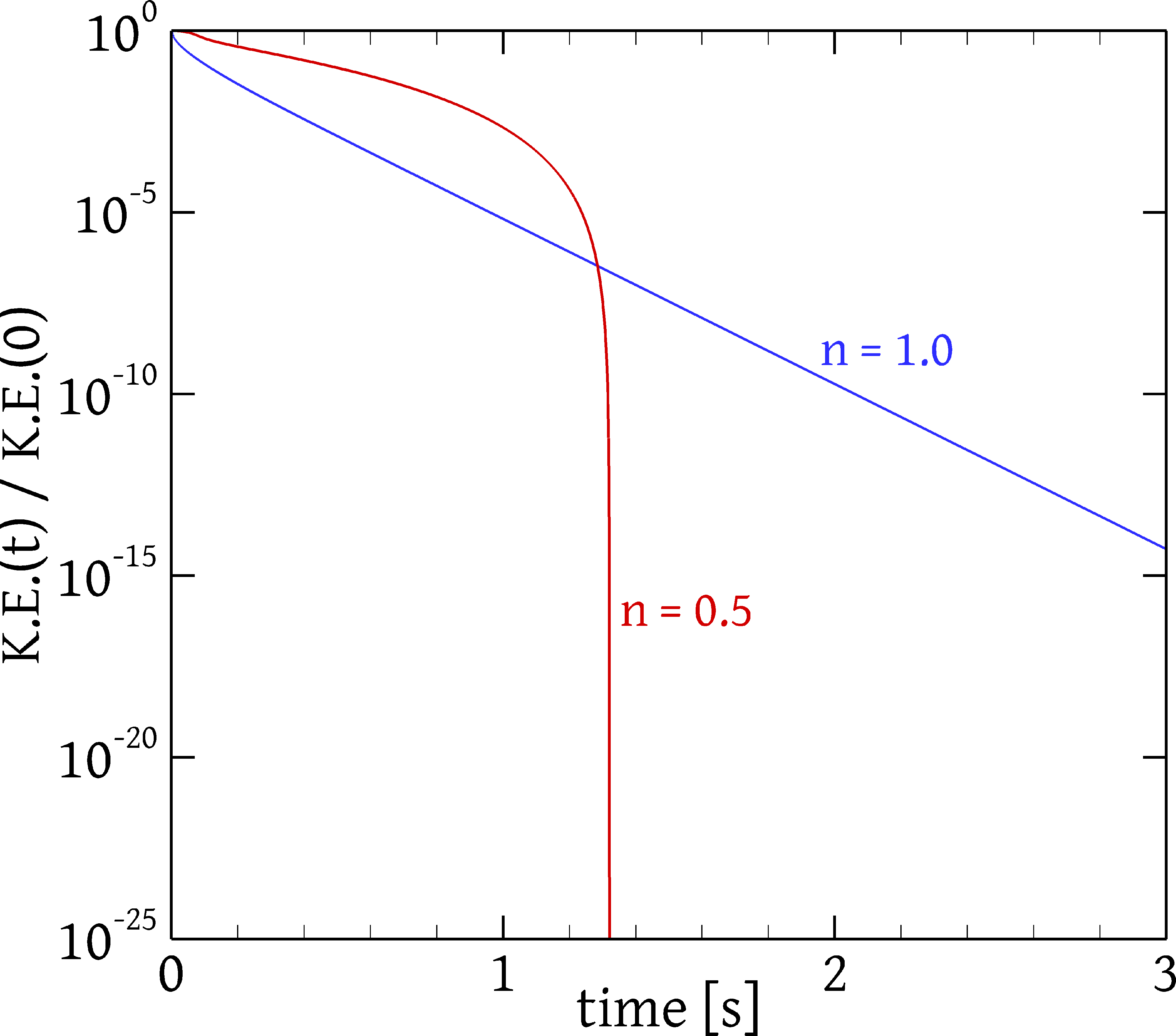
Figure 27: Decay of kinetic energy with time after lid motion cessation of two power law fluids (Eq. (1) with $\tau_{y}$ = 0, $k$ = 1 $\mathrm{P}\mathrm{a}\,\mathrm{s}^{n}$, and $\rho$ = 1000 $\mathrm{k}\mathrm{g}\mathrm{/}\mathrm{m}^{3}$) of exponents $n$ = 1.0 and 0.5, respectively. The domain and grid are the same as in Sec. 6, and the initial condition ($t$ = 0) is the steady state flow for a lid velocity of 1 $\mathrm{m}\mathrm{/}\mathrm{s}$. The kinetic energy is normalised by its value at $t$ = 0. The lid is brought to a halt suddenly for $n$ = 1, but gradually over a time interval of 0.1 $\mathrm{s}$ for $n$ = 0.5 (to avoid iterative solver convergence difficulties).

Appendix D Second order accurate reconstruction of cell centre value from face values

Suppose that the exact (or approximated to at least second-order accuracy) values $\phi_{f}$ of a quantity $\phi$ are known at the face centres of a cell $P$ (Fig. 2), and we want to approximate from these values the value of $\phi$ at the cell centre, $\overline{\phi_{P}}$. One way to proceed is the following. The fact that the known values are located at the cell boundary provides an incentive to try to derive a scheme based on the divergence theorem. Let $\underline{r}(\underline{x})=\underline{x}-\underline{P}$ be the vector function that returns the relative position of location $\underline{x}$ relative to the centroid $\underline{P}$. Then $\nabla\cdot\underline{r}=\nabla\cdot\underline{x}=D$ where $D=2$ or 3 in two- and three-dimensional space, respectively. We can then use the product rule to the divergence of the product $\phi\underline{r}$:

$$\nabla\cdot(\phi\underline{r})\;=\;\nabla\phi\cdot\underline{r}\;+\;\phi\,\nabla\cdot\underline{r}\;=\;\nabla\phi\cdot\underline{r}\;+\;D\,\phi$$

Integrating both sides over the whole cell $P$ and applying the divergence theorem on the left-hand side we get

$$\sum_{f=1}^{F}\int_{s_{f}}\phi\,\underline{r}\cdot\underline{n}_{f}\,\mathrm{d}s\;=\;\int_{\Omega_{P}}\nabla\phi\cdot\underline{r}\,\mathrm{d}\Omega\;+\;D\int_{\Omega_{P}}\phi\,\mathrm{d}\Omega$$ (D.1)

This is an exact equation, but now we will approximate each of the integrals by the midpoint rule:

$$\int_{s_{f}}\phi\,\underline{r}\cdot\underline{n}_{f}\,\mathrm{d}s\; =\;\phi(\underline{c}_{f})\,(\underline{r}(\underline{c}_{f})\cdot\underline{n}_{f})\,s_{f}\;+\;O(h^{2})\,s_{f}$$ (D.2)

$$\int_{\Omega_{P}}\nabla\phi\cdot\underline{r}\,\mathrm{d}\Omega\; =\;\nabla\phi(\underline{P})\cdot\underline{r}(\underline{P})\,\Omega_{P}\;+\;O(h^{2})\,\Omega_{P}\;=\;0\;+\;O(h^{2})\,\Omega_{P}$$ (D.3)

$$\int_{\Omega_{P}}\phi\,\mathrm{d}\Omega\; =\;\phi(\underline{P})\,\Omega_{P}\;+\;O(h^{2})\,\Omega_{P}$$ (D.4)

where in (D.3) we have used that $\underline{r}(\underline{P})=\underline{P}-\underline{P}=0$. Substituting these into (D.1) we get

$$\phi(\underline{P})\;=\;\underbrace{\frac{1}{D\,\Omega_{P}}\sum_{f=1}^{F}\left[\phi(\underline{c}_{f})\,s_{f}\,\underline{r}(\underline{c}_{f})\cdot\underline{n}_{f}\right]}_{\overline{\phi_{P}}}\;+\;\underbrace{\sum_{f=1}^{F}O(h^{2})\frac{s_{f}}{\Omega_{P}}}_{=O(h)}$$ (D.5)

The first term on the right hand side is the approximation $\overline{\phi_{P}}$, as can be seen by comparing to Eq. (59). The second term on the right hand side is the difference between this approximation and the exact value $\phi(\underline{P})$, i.e. the error, which is $O(h)$ because $s_{f}/\Omega_{P}=O(h^{-1})$. Therefore, the approximation (59) appears to be only first-order accurate, of the same order as simply setting $\overline{\phi_{P}}=\phi(\underline{c}_{f})$ for any arbitrary face $f$!

Is it possible that this error estimation is too pessimistic and does not account for some error cancellation that occurs when adding the truncation errors of the midpoint rule approximations (D.2) – (D.4)? In fact this happens to be the case and it turns out that the approximation (59) is second-order accurate, which is easiest to prove by showing that it is exact for linear functions. Indeed, if it is exact for linear functions then expanding $\phi$ in a Taylor series about $\underline{P}$ we find that the error is

$$\phi(\underline{x})\; =\;\phi(\underline{P})\;+\;\nabla\phi(\underline{P})\cdot\underline{r}(\underline{x})\;+\;O(h^{2})\;\Rightarrow$$

$$\overline{\phi_{P}}\; =\;\overline{[\phi(\underline{P})\;+\;\nabla\phi(\underline{P})\cdot\underline{r}(\underline{x})]_{P}}\;+\;\overline{O(h^{2})_{P}}$$

$$=\;\phi(\underline{P})\;+\;\nabla\phi(\underline{P})\cdot\underline{r}(\underline{P})\;+\;\overline{O(h^{2})_{P}}$$

$$=\;\phi(\underline{P})\;+\;O(h^{2})$$

where we have used the facts that our interpolation operator (59) is linear ($\overline{[\phi+\psi]_{P}}=\overline{\phi_{P}}+\overline{\psi_{P}}$), that it is exact for linear functions (and $\phi(\underline{P})+\nabla\phi(\underline{P})\cdot\underline{r}(\underline{x})$ is a linear function), that $\underline{r}(\underline{P})=0$, and finally that $\overline{O(h^{2})_{P}}=O(h^{2})$ (which can be seen by replacing $\tau_{ij,f}$ with $O(h^{2})$ in the formula (59) and noting that both $s_{f}(\underline{c}_{f}-\underline{P})\cdot\underline{n}_{f}$ and $\Omega_{P}$ are of the same order, $O(h^{2})$ in 2D and $O(h^{3})$ in 3D).

It remains to show that the interpolation operator is exact for linear functions. Suppose a linear function $\phi(\underline{x})=\phi(\underline{P})+\underline{g}\cdot\underline{r}(\underline{x})$ where $\underline{g}$ is a constant vector (it is the gradient of $\phi$). We want to show that $\overline{\phi_{P}}=\phi(\underline{P})$. Applying the approximation (59) to $\phi$ we get

$$\overline{\phi_{P}}\; =\;\frac{1}{D\,\Omega_{P}}\sum_{f=1}^{F}\left[\left(\phi(\underline{P})+\underline{g}\cdot\underline{r}(\underline{c}_{f})\right)(\underline{r}(\underline{c}_{f})\cdot\underline{n}_{f})\,s_{f}\right]$$

$$=\;\phi(\underline{P})\,\frac{1}{D\,\Omega_{P}}\sum_{f=1}^{F}\left[(\underline{r}(\underline{c}_{f})\cdot\underline{n}_{f})\,s_{f}\right]\;+\;\frac{1}{D\,\Omega_{P}}\,\underline{g}\cdot\sum_{f=1}^{F}\left[\underline{r}(\underline{c}_{f})(\underline{r}(\underline{c}_{f})\cdot\underline{n}_{f})\,s_{f}\right]$$ (D.6)

To proceed further we need a couple of geometrical results. Figure 28 shows cell $P$ divided into $F$ triangles by the dashed lines which connect the centroid $\underline{P}$ to the vertices $\underline{v}_{f}$. Consider the triangle $(\underline{P},\underline{v}_{f},\underline{v}_{f+1})$, which has face $f$ as one of its sides. The product $\underline{r}(\underline{c}_{f})\cdot\underline{n}_{f}$ is the perpendicular distance from $\underline{P}$ to face $f$, and therefore the product $(\underline{r}(\underline{c}_{f})\cdot\underline{n}_{f})\,s_{f}$ is equal to the shaded area of Fig. 28, which is enclosed in a rectangle with one side coinciding with face $f$, another parallel side through $\underline{P}$, and two perpendicular sides passing through the vertices $\underline{v}_{f}$ and $\underline{v}_{f+1}$, respectively. The area of the triangle $(\underline{P},\underline{v}_{f},\underline{v}_{f+1})$ is half that of this rectangle (in three dimensions, the volume of the cone-like shape obtained by joining $\underline{P}$ with the edges of face $f$ is one third of the volume of the shaded rectangular box). By adding the areas of all triangles we get the total area of cell $P$:

$$\frac{1}{D}\sum_{f=1}^{F}\left(\underline{r}(\underline{c}_{f})\cdot\underline{n}_{f}\right)s_{f}\;=\;\Omega_{P}$$ (D.7)

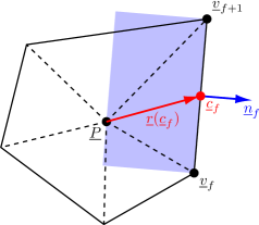
Figure 28: Notation concerning the geometry of cell $P$.

A second geometric result that will be needed is the following. The centroid of the triangle $(\underline{P},\underline{v}_{f},\underline{v}_{f+1})$ is $(\underline{P}+\underline{v}_{f}+\underline{v}_{f+1})/3=(\underline{P}+2\underline{c}_{f})/3$. The centroid of the whole cell, $\underline{P}$, is equal to the sum of the individual centroids of the triangles, $\underline{P}_{f}$ say, weighted by their areas, $\Omega_{f}=(1/2)(\underline{r}(\underline{c}_{f})\cdot\underline{n}_{f})s_{f}$:

$$\underline{P}\;=\;\frac{1}{\Omega_{P}}\sum_{f=1}^{F}\underline{P}_{f}\,\Omega_{f}\;\;\Rightarrow\;\;\underline{P}\Omega_{P}\;=\;\sum_{f=1}^{F}\frac{1}{3}\left(\underline{P}+2\underline{c}_{f}\right)\frac{1}{2}\left(\underline{r}(\underline{c}_{f})\cdot\underline{n}_{f}\right)s_{f}$$

Substituting for $\Omega_{P}$ from (D.7) (with $D=2$), moving everything to the left hand side, and merging the two sums, we arrive at

$$\sum_{f=1}^{F}\underline{r}(\underline{c}_{f})\left(\underline{r}(\underline{c}_{f})\cdot\underline{n}_{f}\right)s_{f}\;=\;0$$ (D.8)

where we have used also that $\underline{c}_{f}-\underline{P}=\underline{r}(\underline{c}_{f})$. In three dimensions, the exact same equation (D.8) holds, but is derived by noting that the volume of the cone- or pyramid-like shape whose base is face $f$ and its apex is at $\underline{P}$ is $\Omega_{f}=(1/3)(\underline{r}(\underline{c}_{f})\cdot\underline{n}_{f})s_{f}$ ($D=3$ in Eq. (D.7)) while its centroid is $\underline{P}_{f}=(\underline{P}+3\underline{c}_{f})/4$.

Finally, substituting Eqs. (D.7) and (D.8) in the first and second terms, respectively, of the right-hand side of Eq. (D.6), we arrive at $\overline{\phi_{P}}=\phi(\underline{P})$: the interpolation scheme (59) is exact for linear functions, and is therefore second-order accurate.

References

- [1] P. Coussot, “Bingham’s heritage,” Rheologica Acta, vol. 56, pp. 163–176, 2017.
- [2] P. Coussot, “Slow flows of yield stress fluids: yielding liquids or flowing solids?,” Rheologica Acta, vol. 57, pp. 1–14, 2018.
- [3] D. Bonn, M. M. Denn, L. Berthier, T. Divoux, and S. Manneville, “Yield stress materials in soft condensed matter,” Reviews of Modern Physics, vol. 89, 2017.
- [4] E. C. Bingham, Fluidity and Plasticity. McGraw-Hill, 1922.
- [5] W. H. Herschel and R. Bulkley, “Konsistenzmessungen von gummi-benzollösungen,” Kolloid-Zeitschrift, vol. 39, pp. 291–300, 1926.
- [6] K. v. Hohenemser and W. Prager, “Über die ansätze der mechanik isotroper kontinua,” ZAMM-Journal of Applied Mathematics and Mechanics/Zeitschrift für Angewandte Mathematik und Mechanik, vol. 12, pp. 216–226, 1932.
- [7] P. Saramito, “A damped newton algorithm for computing viscoplastic fluid flows,” Journal of Non-Newtonian Fluid Mechanics, vol. 238, pp. 6–15, 2016.
- [8] E. Mitsoulis and J. Tsamopoulos, “Numerical simulations of complex yield-stress fluid flows,” Rheologica Acta, vol. 56, pp. 231–258, 2017.
- [9] P. Saramito and A. Wachs, “Progress in numerical simulation of yield stress fluid flows,” Rheologica Acta, vol. 56, pp. 211–230, 2017.
- [10] Y. Dimakopoulos, G. Makrigiorgos, G. Georgiou, and J. Tsamopoulos, “The PAL (Penalized Augmented Lagrangian) method for computing viscoplastic flows: A new fast converging scheme,” Journal of Non-Newtonian Fluid Mechanics, vol. 256, pp. 23–41, 2018.
- [11] J. Piau, “Carbopol gels: Elastoviscoplastic and slippery glasses made of individual swollen sponges: Meso- and macroscopic properties, constitutive equations and scaling laws,” Journal of Non-Newtonian Fluid Mechanics, vol. 144, pp. 1–29, 2007.
- [12] M. Dinkgreve, M. M. Denn, and D. Bonn, ““everything flows?”: elastic effects on startup flows of yield-stress fluids,” Rheologica Acta, vol. 56, pp. 189–194, 2017.
- [13] N. Dubash and I. Frigaard, “Propagation and stopping of air bubbles in Carbopol solutions,” Journal of Non-Newtonian Fluid Mechanics, vol. 142, pp. 123–134, 2007.
- [14] W. F. Lopez, M. F. Naccache, and P. R. de Souza Mendes, “Rising bubbles in yield stress materials,” Journal of Rheology, vol. 62, pp. 209–219, 2018.
- [15] J. Tsamopoulos, Y. Dimakopoulos, N. Chatzidai, G. Karapetsas, and M. Pavlidis, “Steady bubble rise and deformation in newtonian and viscoplastic fluids and conditions for bubble entrapment,” Journal of Fluid Mechanics, vol. 601, 2008.
- [16] Y. Dimakopoulos, M. Pavlidis, and J. Tsamopoulos, “Steady bubble rise in Herschel–Bulkley fluids and comparison of predictions via the Augmented Lagrangian Method with those via the Papanastasiou model,” Journal of Non-Newtonian Fluid Mechanics, vol. 200, pp. 34–51, 2013.
- [17] D. Fraggedakis, M. Pavlidis, Y. Dimakopoulos, and J. Tsamopoulos, “On the velocity discontinuity at a critical volume of a bubble rising in a viscoelastic fluid,” Journal of Fluid Mechanics, vol. 789, pp. 310–346, 2016.
- [18] D. Fraggedakis, Y. Dimakopoulos, and J. Tsamopoulos, “Yielding the yield-stress analysis: a study focused on the effects of elasticity on the settling of a single spherical particle in simple yield-stress fluids,” Soft Matter, vol. 12, pp. 5378–5401, 2016.
- [19] P. Saramito, “A new constitutive equation for elastoviscoplastic fluid flows,” Journal of Non-Newtonian Fluid Mechanics, vol. 145, pp. 1–14, 2007.
- [20] P. R. de Souza Mendes and R. L. Thompson, “A critical overview of elasto-viscoplastic thixotropic modeling,” Journal of Non-Newtonian Fluid Mechanics, vol. 187-188, pp. 8–15, 2012.
- [21] D. Fraggedakis, Y. Dimakopoulos, and J. Tsamopoulos, “Yielding the yield stress analysis: A thorough comparison of recently proposed elasto-visco-plastic (EVP) fluid models,” Journal of Non-Newtonian Fluid Mechanics, vol. 238, pp. 170–188, 2016.
- [22] I. Cheddadi and P. Saramito, “A new operator splitting algorithm for elastoviscoplastic flow problems,” Journal of Non-Newtonian Fluid Mechanics, vol. 202, pp. 13–21, 2013.
- [23] S. L. Frey, M. F. Naccache, P. R. de Souza Mendes, R. L. Thompson, D. D. dos Santos, F. B. Link, and C. Fonseca, “Performance of an elasto-viscoplastic model in some benchmark problems,” Mechanics of Time-Dependent Materials, vol. 19, pp. 419–438, 2015.
- [24] A. Syrakos, G. Georgiou, and A. Alexandrou, “Solution of the square lid-driven cavity flow of a Bingham plastic using the finite volume method,” Journal of Non-Newtonian Fluid Mechanics, vol. 195, pp. 19–31, 2013.
- [25] A. Syrakos, Y. Dimakopoulos, G. C. Georgiou, and J. Tsamopoulos, “Viscoplastic flow in an extrusion damper,” Journal of Non-Newtonian Fluid Mechanics, vol. 232, pp. 102–124, 2016.
- [26] P. J. Oliveira, F. T. Pinho, and G. A. Pinto, “Numerical simulation of non-linear elastic flows with a general collocated finite-volume method,” Journal of Non-Newtonian Fluid Mechanics, vol. 79, pp. 1–43, 1998.
- [27] J. L. Favero, A. R. Secchi, N. S. M. Cardozo, and H. Jasak, “Viscoelastic flow analysis using the software OpenFOAM and differential constitutive equations,” Journal of Non-Newtonian Fluid Mechanics, vol. 165, pp. 1625–1636, 2010.
- [28] A. Afonso, M. Oliveira, P. Oliveira, M. Alves, and F. Pinho, “The finite-volume method in computational rheology,” in Finite-Volume Methods - Powerful Means of Engineering Design, ch. 7, pp. 141–170, In-Tech Open Publishers, 2012.
- [29] A. Syrakos, Y. Dimakopoulos, and J. Tsamopoulos, “Theoretical study of the flow in a fluid damper containing high viscosity silicone oil: Effects of shear-thinning and viscoelasticity,” Physics of Fluids, vol. 30, p. 030708, 2018.
- [30] F. Belblidia, H. R. Tamaddon-Jahromi, M. F. Webster, and K. Walters, “Computations with viscoplastic and viscoelastoplastic fluids,” Rheologica Acta, vol. 50, pp. 343–360, 2011.
- [31] P. Saramito, “A new elastoviscoplastic model based on the Herschel–Bulkley viscoplastic model,” Journal of Non-Newtonian Fluid Mechanics, vol. 158, pp. 154–161, 2009.
- [32] I. Cheddadi, P. Saramito, and F. Graner, “Steady Couette flows of elastoviscoplastic fluids are nonunique,” Journal of Rheology, vol. 56, pp. 213–239, 2012.
- [33] L. Lacaze, A. Filella, and O. Thual, “Steady and unsteady shear flows of a viscoplastic fluid in a cylindrical Couette cell,” Journal of Non-Newtonian Fluid Mechanics, vol. 220, pp. 126–136, 2015.
- [34] A. Syrakos, G. C. Georgiou, and A. N. Alexandrou, “Performance of the finite volume method in solving regularised Bingham flows: Inertia effects in the lid-driven cavity flow,” Journal of Non-Newtonian Fluid Mechanics, vol. 208–209, pp. 88–107, 2014.
- [35] R. Sousa, R. Poole, A. Afonso, F. Pinho, P. Oliveira, A. Morozov, and M. Alves, “Lid-driven cavity flow of viscoelastic liquids,” Journal of Non-Newtonian Fluid Mechanics, vol. 234, pp. 129–138, 2016.
- [36] R. da R. Martins, G. M. Furtado, D. D. dos Santos, S. Frey, M. F. Naccache, and P. R. de Souza Mendes, “Elastic and viscous effects on flow pattern of elasto-viscoplastic fluids in a cavity,” Mechanics Research Communications, vol. 53, pp. 36–42, 2013.
- [37] A. Syrakos, G. C. Georgiou, and A. N. Alexandrou, “Thixotropic flow past a cylinder,” Journal of Non-Newtonian Fluid Mechanics, vol. 220, pp. 44–56, 2015.
- [38] C. J. Dimitriou and G. H. McKinley, “A comprehensive constitutive law for waxy crude oil: a thixotropic yield stress fluid,” Soft Matter, vol. 10, pp. 6619–6644, 2014.
- [39] I. Cheddadi, P. Saramito, C. Raufaste, P. Marmottant, and F. Graner, “Numerical modelling of foam Couette flows,” The European Physical Journal E, vol. 27, 2008.
- [40] A. Syrakos, G. C. Georgiou, and A. N. Alexandrou, “Cessation of the lid-driven cavity flow of Newtonian and Bingham fluids,” Rheologica Acta, vol. 55, pp. 51–66, 2016.
- [41] R. L. Thompson and E. J. Soares, “Viscoplastic dimensionless numbers,” Journal of Non-Newtonian Fluid Mechanics, vol. 238, pp. 57–64, 2016.
- [42] A. Syrakos and A. Goulas, “Estimate of the truncation error of finite volume discretization of the Navier-Stokes equations on colocated grids,” International Journal for Numerical Methods in Fluids, vol. 50, pp. 103–130, 2006.
- [43] J. Sun, M. Smith, R. Armstrong, and R. Brown, “Finite element method for viscoelastic flows based on the discrete adaptive viscoelastic stress splitting and the discontinuous Galerkin method: DAVSS-G/DG,” Journal of Non-Newtonian Fluid Mechanics, vol. 86, pp. 281–307, 1999.
- [44] A. Syrakos, S. Varchanis, Y. Dimakopoulos, A. Goulas, and J. Tsamopoulos, “A critical analysis of some popular methods for the discretisation of the gradient operator in finite volume methods,” Physics of Fluids, vol. 29, p. 127103, 2017.
- [45] C. M. Rhie and W. L. Chow, “Numerical study of the turbulent flow past an airfoil with trailing edge separation,” AIAA Journal, vol. 21, pp. 1525–1532, 1983.
- [46] S. Zhang, X. Zhao, and S. Bayyuk, “Generalized formulations for the Rhie–Chow interpolation,” Journal of Computational Physics, vol. 258, pp. 880–914, 2014.
- [47] G. B. Deng, J. Piquet, P. Queutey, and M. Visonneau, “Incompressible flow calculations with a consistent physical interpolation finite volume approach,” Computers & fluids, vol. 23, pp. 1029–1047, 1994.
- [48] C. Klaij, “On the stabilization of finite volume methods with co-located variables for incompressible flow,” Journal of Computational Physics, vol. 297, pp. 84–89, 2015.
- [49] H. M. Matos, M. A. Alves, and P. J. Oliveira, “New formulation for stress calculation: Application to viscoelastic flow in a T-junction,” Numerical Heat Transfer, Part B: Fundamentals, vol. 56, pp. 351–371, 2009.
- [50] M. Niethammer, H. Marschall, C. Kunkelmann, and D. Bothe, “A numerical stabilization framework for viscoelastic fluid flow using the finite volume method on general unstructured meshes,” International Journal for Numerical Methods in Fluids, vol. 86, pp. 131–166.
- [51] F. Pimenta and M. Alves, “Stabilization of an open-source finite-volume solver for viscoelastic fluid flows,” Journal of Non-Newtonian Fluid Mechanics, vol. 239, pp. 85–104, 2017.
- [52] C. Fernandes, M. S. B. Araujo, L. L. Ferras, and J. M. Nobrega, “Improved both sides diffusion (iBSD): A new and straightforward stabilization approach for viscoelastic fluid flows,” Journal of Non-Newtonian Fluid Mechanics, vol. 249, pp. 63–78, 2017.
- [53] A. Syrakos, G. Efthimiou, J. G. Bartzis, and A. Goulas, “Numerical experiments on the efficiency of local grid refinement based on truncation error estimates,” Journal of Computational Physics, vol. 231, pp. 6725–6753, 2012.
- [54] S. Patankar, Numerical heat transfer and fluid flow. CRC press, 1980.
- [55] J. H. Ferziger and M. Peric, Computational methods for fluid dynamics. Springer, 3rd ed., 2002.
- [56] F. Habla, A. Woitalka, S. Neuner, and O. Hinrichsen, “Development of a methodology for numerical simulation of non-isothermal viscoelastic fluid flows with application to axisymmetric 4:1 contraction flows,” Chemical Engineering Journal, vol. 207-208, pp. 772–784, 2012.
- [57] F. Moukalled, L. Mangani, and M. Darwish, The Finite Volume Method in Computational Fluid Dynamics. Springer, 2016.
- [58] M. A. Alves, P. J. Oliveira, and F. T. Pinho, “A convergent and universally bounded interpolation scheme for the treatment of advection,” International Journal for Numerical Methods in Fluids, vol. 41, pp. 47–75, 2003.
- [59] X. Chen, H. Marschall, M. Schäfer, and D. Bothe, “A comparison of stabilisation approaches for finite-volume simulation of viscoelastic fluid flow,” International Journal of Computational Fluid Dynamics, vol. 27, pp. 229–250, 2013.
- [60] F. Habla, M. W. Tan, J. Haßlberger, and O. Hinrichsen, “Numerical simulation of the viscoelastic flow in a three-dimensional lid-driven cavity using the log-conformation reformulation in OpenFOAM®,” Journal of Non-Newtonian Fluid Mechanics, vol. 212, pp. 47–62, 2014.
- [61] R. Comminal, J. Spangenberg, and J. H. Hattel, “Robust simulations of viscoelastic flows at high weissenberg numbers with the streamfunction/log-conformation formulation,” Journal of Non-Newtonian Fluid Mechanics, vol. 223, pp. 37–61, 2015.
- [62] P. H. Gaskell and A. K. C. Lau, “Curvature-compensated convective transport: SMART, a new boundedness- preserving transport algorithm,” International Journal for Numerical Methods in Fluids, vol. 8, pp. 617–641.
- [63] H. Jasak, H. Weller, and A. Gosman, “High resolution NVD differencing scheme for arbitrarily unstructured meshes,” International Journal for Numerical Methods in Fluids, vol. 31, pp. 431–449.
- [64] B. P. Leonard, “Bounded hihigh-order upwind multidimensional finite-volume convection-diffusion algorithms,” in Advances in Numerical Heat Transfer (W. J. Minkowycz and E. M. Sparrow, eds.), vol. 1, pp. 1–57, Taylor and Francis, 1996.
- [65] W. Zhou, J. Ouyang, X. Wang, J. Su, and B. Yang, “Numerical simulation of viscoelastic fluid flows using a robust FVM framework on triangular grid,” Journal of Non-Newtonian Fluid Mechanics, vol. 236, pp. 18–34, 2016.
- [66] R. Fattal and R. Kupferman, “Constitutive laws for the matrix-logarithm of the conformation tensor,” Journal of Non-Newtonian Fluid Mechanics, vol. 123, pp. 281–285, 2004.
- [67] A. Afonso, P. J. Oliveira, F. T. Pinho, and M. A. Alves, “The log-conformation tensor approach in the finite-volume method framework,” Journal of Non-Newtonian Fluid Mechanics, vol. 157, no. 1-2, pp. 55–65, 2009.
- [68] F. D. Vita, M. Rosti, D. Izbassarov, L. Duffo, O. Tammisola, S. Hormozi, and L. Brandt, “Elastoviscoplastic flows in porous media,” Journal of Non-Newtonian Fluid Mechanics, vol. 258, pp. 10–21, 2018.
- [69] Y. Dimakopoulos and J. Tsamopoulos, “A quasi-elliptic transformation for moving boundary problems with large anisotropic deformations,” Journal of Computational Physics, vol. 192, pp. 494–522, 2003.
- [70] A. Syrakos and A. Goulas, “Finite volume adaptive solutions using SIMPLE as smoother,” International Journal for Numerical Methods in Fluids, vol. 52, pp. 1215–1245, 2006.
- [71] T.-W. Pan, J. Hao, and R. Glowinski, “On the simulation of a time-dependent cavity flow of an Oldroyd-B fluid,” International Journal for Numerical Methods in Fluids, vol. 60, pp. 791–808, 2009.
- [72] P. Saramito, “On a modified non-singular log-conformation formulation for Johnson–Segalman viscoelastic fluids,” Journal of Non-Newtonian Fluid Mechanics, vol. 211, pp. 16–30, 2014.
- [73] M. A. Hulsen, R. Fattal, and R. Kupferman, “Flow of viscoelastic fluids past a cylinder at high weissenberg number: Stabilized simulations using matrix logarithms,” Journal of Non-Newtonian Fluid Mechanics, vol. 127, pp. 27–39, 2005.
- [74] A. Poumaere, M. Moyers-González, C. Castelain, and T. Burghelea, “Unsteady laminar flows of a Carbopol gel in the presence of wall slip,” Journal of Non-Newtonian Fluid Mechanics, vol. 205, pp. 28–40, 2014.
- [75] T. C. Papanastasiou, “Flows of materials with yield,” Journal of Rheology, vol. 31, pp. 385–404, 1987.
- [76] K. Sverdrup, N. Nikiforakis, and A. Almgren, “Highly parallelisable simulations of time-dependent viscoplastic fluid flow with structured adaptive mesh refinement,” Physics of Fluids, vol. 30, p. 093102, 2018.
- [77] M. R. Hashemi, M. T. Manzari, and R. Fatehi, “Non-linear stress response of non-gap-spanning magnetic chains suspended in a newtonian fluid under oscillatory shear test: A direct numerical simulation,” Physics of Fluids, vol. 29, p. 107106, 2017.
- [78] J. Pérez-González, J. J. López-Durán, B. M. Marín-Santibáñez, and F. Rodríguez-González, “Rheo-PIV of a yield-stress fluid in a capillary with slip at the wall,” Rheologica Acta, vol. 51, pp. 937–946, 2012.
- [79] D. M. Kalyon, “Apparent slip and viscoplasticity of concentrated suspensions,” Journal of Rheology, vol. 49, pp. 621–640, 2005.
- [80] P. Panaseti, A.-L. Vayssade, G. C. Georgiou, and M. Cloitre, “Confined viscoplastic flows with heterogeneous wall slip,” Rheologica Acta, vol. 56, pp. 539–553, 2017.
- [81] P. Panaseti, K. D. Housiadas, and G. C. Georgiou, “Newtonian Poiseuille flows with pressure-dependent wall slip,” Journal of Rheology, vol. 57, pp. 315–332, 2013.
- [82] S. G. Hatzikiriakos, “Wall slip of molten polymers,” Progress in Polymer Science, vol. 37, pp. 624–643, 2012.
- [83] M. Philippou, Y. Damianou, X. Miscouridou, and G. C. Georgiou, “Cessation of newtonian circular and plane couette flows with wall slip and non-zero slip yield stress,” Meccanica, vol. 52, pp. 2081–2099, 2017.
- [84] I. A. Frigaard, Background Lectures on Ideal Visco-Plastic Fluid Flows, pp. 1–40. Springer International Publishing, 2019.
- [85] R. Glowinski, Numerical methods for nonlinear variational problems. Springer-Verlag, 1984.
- [86] R. Huilgol, B. Mena, and J. Piau, “Finite stopping time problems and rheometry of Bingham fluids,” Journal of non-Newtonian Fluid Mechanics, vol. 102, pp. 97–107, 2002.
- [87] L. Muravleva, E. Muravleva, G. C. Georgiou, and E. Mitsoulis, “Unsteady circular Couette flow of a Bingham plastic with the Augmented Lagrangian Method,” Rheologica Acta, vol. 49, pp. 1197–1206, 2010.
- [88] H. H. Winter, “Viscous dissipation term in energy equations,” in Modular Instruction Series C: Calculation and Measurement Techniques for Momentum, Energy and Mass Transfer, Vol. 7, pp. 27–34, American Institute of Chemical Engineers: New York, 1987.
- [89] S. Varchanis, A. Syrakos, Y. Dimakopoulos, and J. Tsamopoulos, “A new Finite Element formulation for viscoelastic flows: circumventing simultaneously the LBB condition and the high-Weissenberg number problem,” Submitted to the Journal of non-Newtonian Fluid Mechanics, vol. x, p. x, 2019.