justified

Shortcut to Equilibration of an Open Quantum System

Abstract

We present a procedure to accelerate the relaxation of an open quantum system towards its equilibrium state. The control protocol, termed Shortcut to Equilibration, is obtained by reverse-engineering the non-adiabatic master equation. This is a non-unitary control task aimed at rapidly changing the entropy of the system. Such a protocol serves as a shortcut to an abrupt change in the Hamiltonian, i.e., a quench. As an example, we study the thermalization of a particle in a harmonic well. We observe that for short protocols there is a three orders of magnitude improvement in accuracy.

Introduction

Equilibration is a natural process, describing the return of a perturbed system back to a thermal state. The relaxation to equilibrium is present in both the classical Fermi (1956); Hecht (1990); Martínez et al. (2016) and quantum Breuer et al. (2002) regimes. Gaining control over the relaxation rate of quantum systems is crucial for enhancing the performance of quantum heat devices Alicki (1979); Kosloff and Rezek (2017); Geva and Kosloff (1992); Feldmann and Kosloff (2003); Dambach et al. (2018). In addition, fast relaxation is beneficial for quantum state preparation Verstraete et al. (2009); Ye et al. (2008) and open system control Koch (2016); Blaquiere et al. (1987); Huang et al. (1983); Brockett et al. (1983); d’Alessandro (2007); Brif et al. (2010). To address these issues, we present a scheme to accelerate the equilibration of an open quantum system, serving as a shortcut to the natural relaxation time $\tau_{R}$. The protocol is termed Shortcut To Equilibration (STE).

This control problem is embedded in the theory of open quantum systems Breuer et al. (2002). The framework of the theory assumes a composite system, partitioned into a system and an external bath. The Hamiltonian describing the evolution of the composite system reads $\hat{H}\left({t}\right)=\hat{H}_{S}\left({t}\right)+\hat{H}_{B}+\hat{H}_{I}$, where $\hat{H}_{S}\left({t}\right)$ is the system Hamiltonian, $\hat{H}_{B}$ is the bath Hamiltonian and $\hat{H}_{I}$ is the system-bath interaction term. When the system depends explicitly on time, the driving protocol influences the system-bath coupling operators and consequently, the relaxation time.

Quantum control in open systems has been addressed in the past utilizing measurement and feedback Lloyd and Viola (2000); Viola et al. (1999); Liu et al. (2011); Khodjasteh et al. (2010); Schmidt et al. (2011); Altafini (2004). Typically, the effect of non-adiabatic driving on the dissipative dynamics was ignored Vacanti et al. (2014); Suri et al. (2017); Jing et al. (2013); Scandi and Perarnau-Llobet (2018). Here, we present a comprehensive theory that incorporates the non-adiabatic effects. The formalism is based on the recent derivation of the Non Adiabatic Master Equation (NAME) Dann et al. (2018). This master equation is of the Gorini-Kossakowski-Lindblad-Sudarshan (GKLS) form, guaranteeing a complete positive trace-preserving dynamical map Lindblad (1976); Gorini et al. (1976); Alicki (2007). A further prerequisite is the inertial theorem Dann and Kosloff (2018). This theorem allows extending the validity of the NAME for processes with small ‘acceleration’ of the external driving.

We consider a driven quantum system, the Hamiltonian of which varies from $\hat{H}_{S}\left({0}\right)$ to a final Hamiltonian $\hat{H}_{S}\left({t_{f}}\right)$, while coupled to a thermal bath (see Fig. 1). Our aim is to exploit the non-adiabatic effects of the driving to accelerate the system’s return to equilibrium. By reverse-engineering the NAME, we find a protocol that transforms the thermal state of $\hat{H}_{S}\left({0}\right)$ at temperature $T$ to the corresponding thermal state of $\hat{H}_{S}\left({t_{f}}\right)$. This procedure serves as a shortcut for the natural relaxation time $\tau_{R}$.

Controlling the equilibration rate differs from the control tasks treated by shortcuts to adiabaticity Demirplak and Rice (2003); Berry (2009); Chen et al. (2010); Muga et al. (2010); Stefanatos et al. (2010); Hoffmann et al. (2011); del Campo (2013); Torrontegui et al. (2013); Abah and Lutz (2017); Reichle et al. (2006). The latter protocols generate an entropy-preserving unitary transformation, which is effectively the identity map between initial and final diagonal states in the energy representation. Conversely, the STE procedure is a non-unitary transformation, which is designed to rapidly change the entropy of the system.

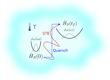
Figure 1: Scheme of the Shortcut To Equilibration (STE) protocol (curved red line) and the quench protocol (blue step line), transforming an initial thermal state at temperature $T$ and frequency $\omega_{i}$ to a final thermal state with an equivalent temperature and frequency $\omega_{f}$.

System dynamics

We consider a quantum particle in contact with a thermal bath while confined by a time-dependent harmonic trap. The system Hamiltonian reads

$$\hat{H}_{S}\left({t}\right)=\frac{\hat{P}^{2}}{2m}+\frac{1}{2}m\omega^{2}\left({t}\right)\hat{Q}^{2}~{},$$ (1)

where $\hat{Q}$ and $\hat{P}$ are the position and momentum operators, respectively, $m$ is the particle mass and $\omega\left({t}\right)$ is the time-dependent oscillator frequency. We assume a Bosonic bath with 1D Ohmic spectral density and an interaction Hamiltonian of the form $\hat{H}_{I}=-\hat{D}\otimes\hat{B}$, where $\hat{D}=d\hat{a}+d^{*}\hat{a}^{\dagger}$ ($a$ and $a^{\dagger}$ are the annihilation and creation operators of the oscillator, respectively), $d$ is the interaction strength and $\hat{B}$ is the bath interaction operator. Throughout the paper, we choose units related to the minimum frequency $\omega_{min}$, time $2\pi/\omega_{min}$ and energy $\hbar\omega_{min}$ with $\hbar=1$.

At initial time, the open quantum system is in equilibrium with the bath, and the state is of a Gibbs canonical form $\hat{\rho}_{S}\left({0}\right)=Z^{-1}e^{-\hat{H}_{S}\left({0}\right)/k_{B}T}$, where $Z$ is the partition function, $k_{B}$ is the Boltzmann constant and $T$ is the temperature of the bath. We search for a protocol that varies the Hamiltonian toward $\hat{H}_{S}\left({t_{f}}\right)$ with a target thermal state $\hat{\rho}_{S}^{Th}\left({t_{f}}\right)=Z^{-1}e^{-\hat{H}_{S}\left({t_{f}}\right)/k_{B}T}$. This procedure serves as a shortcut to an isothermal process. The accuracy of this transformation can be quantified using the fidelity $\cal{F}$, which is a measure of the distance between the final state $\hat{\rho}_{S}\left({t_{f}}\right)$ of the protocol and $\hat{\rho}_{S}^{Th}\left({t_{f}}\right)$ Isar (2009); Scutaru (1998); Banchi et al. (2015). A classical analogous problem has been addressed by Martinez et al. Martínez et al. (2016).

The most straightforward protocol is a quench protocol. ’Quench’ means abruptly changing the Hamiltonian from $H_{S}\left({0}\right)$ to $H_{S}\left({t_{f}}\right)$, and then letting the system equilibrate with the bath, Cf. Supplemental Material (SM) III. When $\hat{H}_{S}\left({0}\right)$ and $\hat{H}_{S}\left({t_{f}}\right)$ do not commute, which is the case for a non-rigid harmonic oscillator, such a sudden change generates coherence in the energy basis, leading to deviations from equilibrium. The quenched system relaxes at an exponential rate toward equilibrium, which leads to an asymptotic exponential convergence of the fidelity toward unity $1-{\cal{F}}\left({t}\right)\propto e^{-kt}$, for $t/k>1$, with $k=k_{\downarrow}-k_{\uparrow}$, where $k_{\downarrow}$ and $k_{\uparrow}$ are decay rates, Cf. SM IIIA. We use the quench protocol as a benchmark to assess the STE protocol’s performance.

To describe the reduced dynamics under the STE, we follow the derivation presented in Refs. Dann et al. (2018); Dann and Kosloff (2018). First, we obtain a solution for the unitary propagator $\hat{U}_{S}\left({t,0}\right)$ for a protocol determined by a constant adiabatic parameter $\mu=\dot{\omega}/\omega^{2}$. The closed-form solution of $\hat{U}_{S}\left({t,0}\right)$ allows constructing a master equation that includes the bath’s influence on the reduced dynamics. Then, by utilizing the inertial theorem, we extend the description to protocols where $\mu$ varies slowly ($d\mu/dt\ll 1$). This condition sets a lower bound for the minimum protocol duration. For protocols faster than the minimum time, the condition $d\mu/dt\ll 1$ is no longer satisfied and the inertial approximation loses its validity Dann and Kosloff (2018). The bound is given by $t_{f}>f\cdot\text{max}_{s}\left({\frac{1}{\omega}\sqrt{\frac{\omega^{\prime\prime}\left({s}\right)}{2\omega}\frac{1}{8-\mu^{2}}}}\right)$, where $s=t/t_{f}$ and $f<1$ is a small scalar, dependent on the desired precision, Cf. SM II. For example, if $f=0.05$, the lower bound is $t_{f}>4.38\,\,\left({2\pi/\omega_{min}}\right)$, where $\omega_{min}=5\,\text{a.u}$.

The range of validity of the NAME sets a number of conditions: (i) weak coupling between system and bath, which also allows for a reduced description of the system’s dynamics in terms of $\hat{\rho}_{S}$ Breuer et al. (2002); (ii) Markovianity ; (iii) large Bohr frequencies relative to the relaxation rate $\tau_{R}$; (iv) slow driving relative to the decay of the bath correlations. In the following, we consider a regime where the NAME and inertial theorem are valid.

The dynamics of the externally driven open quantum system, in the interaction representation, is described by

$$\frac{d}{dt}\tilde{\rho}_{S}\left({t}\right)=k_{\downarrow}\left({t}\right)\left({\hat{b}\tilde{\rho}_{S}\left({t}\right)\hat{b}^{\dagger}-\frac{1}{2}\{\hat{b}^{\dagger}\hat{b},\tilde{\rho}_{S}\left({t}\right)\}}\right)\\ +k_{\uparrow}\left({t}\right)\left({\hat{b}^{\dagger}\tilde{\rho}_{S}\left({t}\right)\hat{b}-\frac{1}{2}\{\hat{b}\hat{b}^{\dagger},\tilde{\rho}_{S}\left({t}\right)\}}\right)~{}~{}~{}.$$ (2)

Here, the interaction picture density operator reads $\tilde{\rho}_{S}\left({t}\right)=\hat{U}\left({t,0}\right)\hat{\rho}_{S}\left({t}\right)\hat{U}^{\dagger}\left({t,0}\right)$. We use the notation $\tilde{A}$ to describe operators in an interaction picture relative to the system Hamiltonian. For an ohmic Bosonic bath, the decay rates are

$$k_{\downarrow}\left({t}\right)=k_{\uparrow}\left({t}\right)e^{\alpha\left({t}\right)/k_{B}T}=\frac{\alpha\left({t}\right)|\vec{d}|^{2}}{8\pi\varepsilon_{0}\hbar c}\left({1+N\left({\alpha\left({t}\right)}\right)}\right)~{},$$ (3)

where $N$ is the occupation number of the Bose-Einstein distribution and $\alpha$ is a modified frequency, determined by the non-adiabatic driving protocol Dann et al. (2018). In terms of the oscillator frequency, the modified frequency is given by

$$\alpha\left({t}\right)=\sqrt{1-\frac{1}{4}\left({\frac{\dot{\omega}\left({t}\right)}{\omega^{2}\left({t}\right)}}\right)^{2}}\omega\left({t}\right)~{}~{}.$$ (4)

The Lindblad jump operators become $\hat{b}\equiv\hat{b}\left({0}\right)=\sqrt{\frac{m\omega\left({0}\right)}{2\hbar}}\frac{\left(\kappa+i\mu\right)}{\kappa}\left({\hat{Q}\left({0}\right)+\frac{\mu+i\kappa}{2m\omega\left({0}\right)}\hat{P}\left({0}\right)}\right)$ where $\kappa=\sqrt{4-\mu^{2}}$.

In the interaction representation the Lindblad operators are time-independent. This property provides an explicit solution in terms of the second-order moments ${\cal{B}}=\{\hat{b}^{\dagger}\hat{b},\hat{b}^{2},\hat{b}^{\dagger 2}\}$ Dann et al. (2018); Dann and Kosloff (2018), Cf. SM I, which, together with the identity operator, form a closed Lie algebra. The solution is given by a generalized canonical state, which has a Gaussian form in terms of $\cal{B}$. Such states are canonical invariant under the dynamics described by Eq. (2), implying that the system can be described by the generalized canonical state throughout the entire evolution Alhassid and Levine (1978); Jaynes (1957); Rezek and Kosloff (2006); Andersen et al. (1964). The system state is given by

$$\tilde{\rho}_{S}\left({t}\right)=Z^{-1}e^{\gamma\left({t}\right)\tilde{b}^{2}}e^{\beta\left({t}\right)\tilde{b}^{\dagger}\tilde{b}}e^{\gamma^{*}\left({t}\right)\tilde{b}^{\dagger 2}}~{}~{},$$ (5)

which is completely defined by the time-dependent coefficients $\gamma$ and $\beta$ and the driving protocol. The partition function reads $Z\left({\beta,\gamma}\right)=\frac{e^{-\beta}}{\left({e^{-\beta}-1}\right)\sqrt{1-4|\gamma|^{2}/\left({e^{-\beta}-1}\right)^{2}}}$. In the adiabatic limit, the adiabatic parameter $\mu$ approaches zero, the state follows the adiabatic solution, and $\hat{b}^{\dagger}\hat{b}\rightarrow\hat{a}^{\dagger}\hat{a}$.

Substituting $\tilde{\rho}_{S}\left({t}\right)$ into the master equation, Eq. (2), multiplying by $\tilde{\rho}_{S}^{-1}$ from the right and comparing the terms proportionate to the operators $\tilde{b}^{\dagger}\tilde{b}$, $\tilde{b}^{2}$ and $\tilde{b}^{\dagger 2}$ leads to

$$\begin{array}[]{l}\dot{\beta}=k_{\downarrow}\left({e^{\beta}-1}\right)+k_{\uparrow}\left({e^{-\beta}-1+4e^{\beta}|\gamma|^{2}}\right),\\ \dot{\gamma}=\left({k_{\downarrow}+k_{\uparrow}}\right)\gamma-2k_{\downarrow}\gamma e^{-\beta}~{}~{}.\end{array}$$ (8)

These equations describe the evolution of the system for any initial squeezed thermal state. Here, we assume that the system is in a thermal state at the initial time, which infers $\gamma(0)=0$. This simplifies the expression of the state to

$$\tilde{\rho}_{S}\left({\beta\left({t}\right),\mu\left({t}\right)}\right)=Z^{-1}e^{\beta\hat{b}^{\dagger}\hat{b}\left({\mu}\right)}~{}~{},$$ (9)

and consequently the system dynamics are described by a single non-linear differential equation

$$\dot{\beta}=k_{\downarrow}\left({t}\right)\left({e^{\beta}-1}\right)+k_{\uparrow}\left({t}\right)\left({e^{-\beta}-1}\right)~{}~{},$$ (10)

with initial conditions $\beta\left({0}\right)=-\frac{\hbar\omega\left({0}\right)}{k_{B}T}$ and $\mu\left({0}\right)=0$. Equation (10) constitutes the basis for the suggested control scheme.

Control

The control target is to transform a thermal state, defined by frequency $\omega_{i}$, to a thermal state of frequency $\omega_{f}$, while interacting with a bath at temperature $T$. The control utilizes the fact that at all times, the state is fully defined by $\mu\left({t}\right)$ and $\beta\left({t}\right)$. This property implies $\beta\left({0}\right)=-\frac{\hbar\omega_{i}}{k_{B}T}$, $\beta\left({t_{f}}\right)=-\frac{\hbar\omega_{f}}{k_{B}T}$ and $\mu\left({0}\right)=\mu\left({t_{f}}\right)=0$. The initial and final $\beta$ are connected through Eq. (10), where the protocol defines the rates $k_{\uparrow}\left({t}\right)$ and $k_{\downarrow}\left({t}\right)$. These rates are determined by the parameter $\alpha\left({t}\right)$ in Eq. (3), which in turn is completely defined by the control parameter $\omega\left({t}\right)$ in Eq. (4). Furthermore, $\mu\left({t}\right)$ is determined by $\omega\left({t}\right)$, and therefore $\omega\left({t}\right)$ fully determines the state of the system at all times.

The strategy to solve the control equation is based on a reverse-engineering approach, and the protocol is denoted by Shortcut To Equilibration (STE). The method proceeds as follows: we define a new variable $y=e^{\beta}$, and propose an ansatz for $y$ that satisfies the boundary conditions. Then we solve for $\alpha\left({t}\right)$, and from $\alpha\left({t}\right)$ determine $\omega\left({t}\right)$.

The initial and final thermal states determine the boundary conditions of $\mu\left({t}\right)$, which implies that the state is stationary at initial and final times. This leads to additional boundary conditions $\dot{\beta}\left({0}\right)=\dot{\beta}\left({t_{f}}\right)=0$.

A third-degree polynomial is sufficient to obey all of the constraints. Introducing $s=t/t_{f}$, the solution reads

$$y\left({s}\right)=y\left({0}\right)+3\Delta s^{2}-2\Delta s^{3}~{}~{},$$ (11)

where $\Delta=y\left({t_{f}}\right)-y\left({0}\right)$. In principle, more complicated solutions for Eq. (10) exist; however, here we restrict the analysis to a polynomial solution . The implicit equation for $\alpha\left({t}\right)$ becomes

$$t_{f}\frac{d}{ds}y\left({s}\right)=k_{\downarrow}\left({\alpha\left({s}\right)}\right)y\left({s}\right)^{2}-\\ y\left({s}\right)\left({k_{\downarrow}\left({\alpha\left({s}\right)}\right)+k_{\uparrow}\left({\alpha\left({s}\right)}\right)}\right)+k_{\uparrow}\left({\alpha\left({s}\right)}\right)~{}~{}.$$ (12)

Solving the equation by numerical means generates $\alpha\left({s}\right)$. This solution is substituted into Eq. (4) and the control $\omega\left({t}\right)$ is obtained by an iterative numerical procedure. The protocol satisfies the inertial condition on $\mu$, inferring that the derivation is self-consistent.

The solution of the STE incorporates the adiabatic result in the limit of slow driving. For large protocol time duration ($t_{f}\rightarrow\infty$), the system’s instantaneous state is a thermal state at temperature $T$ with frequency $\omega\left({t}\right)$, see SM IV.

We compare the STE protocol to a quench protocol involving a sudden change from $\omega\left({0}\right)=\omega_{i}$ to $\omega\left({t_{f}}\right)=\omega_{f}$ De Grandi et al. (2010). Two cases are studied, a compression of the potential, which corresponds to the transition $\omega\left({0}\right)=5\rightarrow\omega\left({t_{f}}\right)=10$, and a reversed expansion, associated with the transition $\omega\left({0}\right)=10\rightarrow\omega\left({t_{f}}\right)=5$. Both protocols for each process are presented in Fig. 2 panels (a) and (b). We add, as a reference, an adiabatic process obtained in the limit $t_{f}\rightarrow\infty$. The initial stage of the quench protocol is effectively isolated, as the change in frequency is rapid relative to the relaxation rate toward equilibrium. As a result, the state stays constant while the Hamiltonian abruptly transforms to $\hat{H}_{S}\left({t_{f}}\right)$. Coherence is generated with respect to $\hat{H}\left({t_{f}}\right)$, because $\left[{\hat{H}\left({0}\right),\hat{H}\left({t_{f}}\right)}\right]\neq 0$. After the initial stage energy is exchanged with the bath and the coherence dissipates.

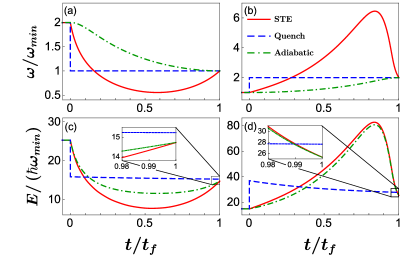
Figure 2: Control protocols as a function of the scaled time $t/t_{f}$: (a,b) the oscillator frequency $\omega$ and (c,d) energy for the STE (red line), quench (dashed blue line) and adiabatic (dot-dashed green line) protocols. (a,c) Expansion, (b,d) compression protocols. The dynamics of the STE and quenched systems are shown for $t_{f}=8\,\text{a.u}$, and the adiabatic dynamics are obtained in the limit $t_{f}\rightarrow\infty$. (c,d) Inset: details of the final approach to the target state. Model parameters (atomic units): $\omega\left({0}\right)/\omega_{f}=5/10$ for the compression, and reverse for the expansion and bath temperature $T=2$.

In figure 3, we compare the fidelity with respect to the target thermal state of the expansion and compression protocols, for increasing stage times $t_{f}$ . The STE protocol transfers the system to the target thermal state with fidelities close to unity ${\cal{F}}\approx 1$, while the quench target has lower fidelity due to the slow relaxation. Therefore, the STE protocol equilibrates the system faster and with higher accuracy than the quench protocol. For a given fidelity, the STE achieves the target state up to five times faster than the quench protocol.

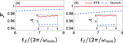
Figure 3: The fidelity of the final state relative to the target thermal state for the short-cut to equilibration (red) and quench (blue) protocols. (a) Expansion protocol, (b) compression protocol. The inset shows the accuracy ${\cal{A}}=-\text{log}_{10}\left({1-{\cal{F}}}\right)$, highlighting the 3-digit accuracy of the STE protocol. Model parameters are the same as in Fig. 2

Figure 2 panels (c) and (d) presents a comparison of the quantum state’s energy for the STE, quench and adiabatic protocols. During the quench protocol, there is a sudden change in the energy, which is followed by a slow exponential decay toward the thermal energy. The adiabatic and STE protocols are characterized by an overshoot beyond the final thermal energy. In the final stage of the STE protocol, the energy rapidly converges to the desired thermal energy, whereas the quenched system remains far from equilibrium (see insets in Fig. 2 panels (c) and (d)).

Energy and entropy cost

A control task can be evaluated by the work and entropy cost required to implement the control. Restrictions on the cost can be connected to quantum friction Feldmann and Kosloff (2003); Plastina et al. (2014), which implies that quicker transformations are accompanied by a higher energy cost Chen and Muga (2010); Hoffmann et al. (2011); Salamon et al. (2009); Campbell and Deffner (2017); Stefanatos (2017). Moreover, in any externally controlled process there is an additional cost in energy and entropy to generate faster driving Torrontegui et al. (2017); Tobalina et al. (2018). The work cost for the STE protocol with a duration time $t$ is defined by the integral form

$$W\left({t}\right)=\int_{0}^{t}{\text{tr}}\left({\hat{\rho}_{S}\left({t^{\prime}}\right)\frac{\partial\hat{H}\left({t^{\prime}}\right)}{\partial t^{\prime}}}\right)dt^{\prime}~{}~{}.$$ (13)

For the quench protocol, the sudden transition occurs on a much faster timescale than the exchange rate of energy with the bath. This implies that the change in internal energy is equal to the work cost.

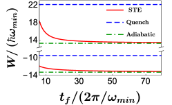
Figure 4: Work required to perform the driving protocol as a function of the normalized time. Model parameters are identical to Fig. 3. Upper part: compression, lower part: expansion.

For the expansion stroke (Fig. 4) the work generated during the STE protocol exceeds the quenched system result, yet remains below the adiabatic limit. When the system is compressed, the STE and quench protocols require additional work compared to the adiabatic process. We can define the efficiency of the process relative to the adiabatic work $W_{adi}$ ($\eta_{comp}=W_{adi}/W$ for compression and $\eta_{exp}=W/W_{adi}$ for the expansion). For the studied case, the efficiency of the STE protocol exceeds that of the quench, $\eta^{quench}_{comp}\approx 0.6$, $\eta^{quench}_{exp}\approx 0.7$, while $\eta^{STE}_{comp}>0.9$ and $\eta^{STE}_{exp}>0.75$, and improves for increasing protocol duration. This result is in accordance with thermodynamic principles, as any rapid driving will induce irreversible dynamics, which in turn leads to sub-optimal performance. For long times, the work of the STE procedure approaches the adiabatic result according to a $t^{-1}$ scaling law. At this limit, the global entropy production approaches zero. For shorter times, the system entropy change, for the STE procedure, is almost independent of protocol duration as a result of the accurate control. The price for shorter protocols is an increase in irreversibility, manifested by larger global entropy production (see SM V).

Discussion

Quantum control is achieved by manipulating the system Hamiltonian via a change of an external control parameter. In turn, the change in the system Hamiltonian influences the system-bath interaction and the equation of motion. Hence, manipulating the Hamiltonian indirectly controls the dissipation rate.

The control procedure employs a closed Lie algebra of system operators. The algebra is used to describe the Hamiltonian, system-bath interaction term and the state. The state is described by a generalized canonical form, Eq. (5); this state is the maximum entropy state constrained by the expectation values of the operators in the algebra. For moderate acceleration of the driving, the inertial theorem can be employed to obtain the non-adiabatic master equation, Eq. (2) Dann et al. (2018, 2018), for which the generalized canonical form of the system state is preserved.

Substituting the generalized canonical form in the equation of motion, Eq. (2), leads to a set of coupled non-linear differential equations of the state parameters, $\gamma$ and $\beta$, which define the generalized canonical state, Eq. (5). These equations completely describe the system dynamics and implicitly depend on the control parameter. They are the basis for the control procedure.

To solve the control problem, we insert a functional form for the state parameters which obeys the correct boundary conditions. Specifically, the parameters are associated with the initial and final thermal states, $\beta\left({0}\right)=-\hbar\omega_{0}/k_{B}T$ and $\beta\left({t_{f}}\right)=-\hbar\omega_{f}/k_{B}T$, with vanishing derivatives at the boundaries. The considered functional form is a third-order polynomial, the coefficients of which are determined by the boundary conditions. This leads to an implicit equation in terms of the control parameter $\omega\left({t}\right)$.

At first glance, it would seem that the quench protocol is optimal, since the approach to equilibrium is exponentially fast. However, a superior solution is obtained by the STE protocol. The advantage of the latter is that it incorporates both the dissipative and unitary parts of the dynamics, changing the rates and engineering the state simultaneously.

The related work cost, required for compression of the harmonic potential or obtained for expansion, is in accordance with thermodynamic principles. These infer that sudden or fast driving of the system increases the power output at the expense of wasted resources and entropy generation.

The STE protocol can be generalized beyond the isothermal example studied here, for three different kinds of scenarios: (i) the temperature of the initial state differs from the bath temperature; (ii) the case of varying bath temperature (with the help of Eq. (3)); (iii) squeezed initial and final states. These general control tasks should be approached by reverse-engineering of both $\beta$ and $\gamma$ in Eq. (8). Furthermore, once a non-adiabatic master equation is obtained Dann et al. (2018); Dann and Kosloff (2018), the method can be generalized to systems characterized by a closed Lie algebra.

To conclude, the STE result demonstrates the feasibility of controlling the entropy of an open quantum system. Such control can be combined with fast unitary transformations to obtain a broad class of states within the system algebra. This will pave the way to faster high-precision quantum control, altering the state’s entropy.

Acknowledgement

We thank KITP for their hospitality, this research was supported in part by the Israel Science Foundation, grant number 2244/14, the National Science Foundation under Grant No. NSF PHY-1748958, the Basque Government, Grant No. IT986- 16 and MINECO/FEDER,UE, Grant No. FIS2015-67161-P. We thank Marcel Fabian and J. Gonzalo Muga for fruitful discussions.

Appendix A Canonical invarience and representation of the system in terms of the generalized Gibbs state coefficients.

We demonstrate how Lie algebra properties and canonical invariance can be utilized to obtain an alternative representation of the system dynamics. For a closed Lie algebra, the system state can be represented in a product form Alhassid and Levine (1978); Jaynes (1957). For the closed set ${\cal{B}}=\{\hat{b}^{\dagger}\hat{b},\hat{b}^{2},\hat{b}^{\dagger 2}\}$ the state is given by a generalized Gibbs state, presented in equation (5) of the Main Part (MP). Next, we calculate ${d\tilde{\rho}_{S}\left({t}\right)}/dt\left({\tilde{\rho}_{S}\left({t}\right)}\right)^{-1}$ explicitly, using the generalized Gibbs state

$$\frac{\partial\tilde{\rho}_{S}\left({t}\right)}{\partial t}\left({\tilde{\rho}_{S}\left({t}\right)}\right)^{-1}\\ =\dot{\gamma}\hat{b}^{2}+\dot{\hat{\beta}}e^{\gamma\hat{b}^{2}}\hat{b}^{\dagger}\hat{b}e^{-\gamma\hat{b}^{2}}+\dot{\gamma}^{*}e^{\gamma\hat{b}^{2}}e^{\beta\hat{b}^{\dagger}\hat{b}}\hat{b}^{\dagger 2}e^{-\beta\hat{b}^{\dagger}\hat{b}}e^{-\gamma\hat{b}^{2}}~{}~{}.$$ (14)

Introducing the Baker–Campbell–Hausdorff relation, leads to

$$\frac{\partial\tilde{\rho}_{S}\left({t}\right)}{\partial t}\left({\tilde{\rho}_{S}\left({t}\right)}\right)^{-1}\\ =\hat{b}^{2}\left({2\dot{\beta}\gamma+\dot{\gamma}+4\gamma^{2}\dot{\gamma}^{*}e^{2\beta}}\right)+\hat{b}^{\dagger}\hat{b}\left({\dot{\beta}+4\gamma\dot{\gamma}^{*}e^{2\beta}}\right)\\ +\hat{b}^{\dagger 2}\dot{\gamma}^{*}e^{2\beta}+\hat{I}2\gamma\dot{\gamma}^{*}e^{2\beta}~{}~{}.$$ (15)

By substituting Eq. (5) MP into the master equation, Eq. (2) MP, we obtain an expansion of ${d\tilde{\rho}_{S}\left({t}\right)}/dt\left({\tilde{\rho}_{S}\left({t}\right)}\right)^{-1}$ in terms of the operators of ${\cal{B}}$. Such a property is termed canonical invariance, it implies that an initial state that belongs to the class of canonical states, will remain in this class throughout the evolution Rezek and Kosloff (2006). The expression reads

$$\frac{\partial\tilde{\rho}_{S}\left({t}\right)}{\partial t}\left({\tilde{\rho}_{S}\left({t}\right)}\right)^{-1}=\hat{b}^{2}A+\hat{b}^{\dagger}\hat{b}B+\hat{b}^{\dagger 2}C+\hat{I}D~{}~{},$$ (16)

where

$$A={k}_{\downarrow}\left({a_{1}-\frac{1}{2}a_{2}}\right)-\frac{1}{2}{k}_{\uparrow}a_{2}$$ (17)

$$B={k}_{\downarrow}\left({b_{1}-\frac{1}{2}b_{2}-\frac{1}{2}}\right)+{k}_{\uparrow}\left({b_{3}-\frac{1}{2}b_{2}-\frac{1}{2}}\right)$$ (18)

$$C=-\frac{1}{2}\left({{k}_{\downarrow}+{k}_{\uparrow}}\right)c_{1}+{k}_{\uparrow}c_{2}$$

$$D={k}_{\downarrow}\left({d_{1}-\frac{1}{2}d_{2}}\right)+{k}_{\uparrow}\left({-\frac{1}{2}\left({d_{3}+1}\right)}\right)~{}~{}.$$

The values of of the coefficients are summarized in Table 1.

Table 1:

coefficient	value	coefficient	value
$a_{1}$	$2\gamma e^{\beta}$	$c_{1}$	$-2\gamma^{*}e^{2\beta}$
$a_{2}$	$2\gamma\left({1-4|\gamma|^{2}e^{2\beta}}\right)$	$c_{2}$	$-2\gamma^{*}e^{\beta}$
$b_{1}$	$e^{\beta}$	$d_{1}$	$e^{\beta}$
$b_{2}$	$1-8|\gamma|^{2}e^{2\beta}$	$d_{2}$	$-4|\gamma|^{2}e^{2\beta}$
$b_{3}$	$e^{-\beta}-4|\gamma|^{2}e^{\beta}$	$d_{3}$	$-2|\gamma|^{2}e^{\beta}+1$

To satisfy both Eq. (15) and (16) the coefficients multiplying each operator must be equal. Comparing terms, leads to four coupled differential equations

$$2\dot{\beta}\gamma+\dot{\gamma}+4\gamma^{2}\dot{\gamma}^{*}e^{2\beta}\\ =\gamma\left(\left(2e^{\beta}-1\right)k_{\downarrow}+4e^{2\beta}\left({k_{\downarrow}+k_{\uparrow}}\right)|\gamma|^{2}-k_{\uparrow}\right)$$ (19)

$$\dot{\beta}+4\gamma\dot{\gamma}^{*}e^{2\beta}=e^{-\beta}\left(\left(e^{\beta}-1\right)\left(e^{\beta}k_{\downarrow}-k_{\uparrow}\right)\right.\\ \left.+4e^{2\beta}|\gamma|^{2}\left(e^{\beta}\left({k_{\downarrow}+k_{\uparrow}}\right)-k_{\uparrow}\right)\right)$$ (20)

$$\dot{\gamma}^{*}e^{2\beta}=k_{\downarrow}e^{2\beta}\gamma^{*}+k_{\uparrow}\gamma^{*}\left({e^{2\beta}-2e^{\beta}}\right)$$ (21)

$$2\gamma\dot{\gamma}^{*}e^{2\beta}=k_{\downarrow}\left({e^{\beta}\left(2e^{\beta}|\gamma|^{2}+1\right)}\right)\\ +k_{\uparrow}\left({2e^{2\beta}|\gamma|^{2}-1}\right)$$ (22)

After some algebraic manipulations we obtain the simplified form

$$\dot{\beta}=k_{\downarrow}\left({e^{\beta}-1}\right)+k_{\uparrow}\left({e^{-\beta}-1+4e^{\beta}|\gamma|^{2}}\right)$$ (23)

$$\dot{\gamma}=\left({k_{\downarrow}+k_{\uparrow}}\right)\gamma-2k_{\downarrow}\gamma e^{-\beta}~{}~{},$$

These coupled differential equations completely determine the system’s dynamics.

Appendix B Lower bound of the protocol duration

The validity of the inertial theorem is quantified by the inertial parameter $\Upsilon$ Dann and Kosloff (2018). When $\Upsilon\ll 1$ the inertial solution is a good approximation of the true dynamics. For the harmonic oscillator, $\Upsilon$ takes the form $\Upsilon\sim\frac{\mu^{\prime}\left({\theta}\right)}{\left({2\kappa}\right)^{2}}$, ($\theta=\theta\left({t}\right)=\int_{0}^{t}\omega\left({t^{\prime}}\right)dt^{\prime}$ and $\kappa=\sqrt{4-\mu^{2}}$), which explicitly becomes

$$\Upsilon=\frac{1}{\left({2\kappa}\right)^{2}}\left({\frac{\ddot{\omega}}{\omega^{3}}-2\mu^{2}}\right)~{}~{}.$$ (24)

Transforming variables to the dimensionless parameter $s=t/t_{f}$ and constraining the inertial parameter by $\Upsilon<f\ll 1$, introduces a lower bound for the protocol duration:

$$t_{f}>f\cdot\text{max}_{s}\left({\frac{1}{\omega}\sqrt{\frac{\omega^{\prime\prime}\left({s}\right)}{2\omega\left({s}\right)}\frac{1}{8-\left({\mu\left({s}\right)}\right)^{2}}}}\right)~{}~{}.$$ (25)

Appendix C Quench protocol

When the parametric quantum harmonic oscillator is in a Gaussian state Jaynes (1957), it is convenient to analyze the system in terms of three time-dependent operators, the Hamiltonian Eq. (1) MP, Lagrangian $\hat{L}\left({t}\right)=\frac{\hat{P}^{2}}{2m}-\frac{1}{2}m\omega^{2}\left({t}\right)\hat{Q}^{2}$, and the position-momentum correlation operator $\hat{C}\left({t}\right)=\frac{\omega\left({t}\right)}{2}\left({\hat{Q}\hat{P}+\hat{P}\hat{Q}}\right)$. The quench protocol includes an initial abrupt shift in frequency from $\omega\left({0}\right)=\omega_{i}$ to $\omega\left({t_{f}}\right)=\omega_{f}$. The sudden transformation is approximately isolated, as the bath’s influence on the system occurs on a much longer timescale. Moreover, for a sudden quench the system state remains unchanged. Hence, time-independent operators, such as $\hat{Q}\left({0}\right)$ and $\hat{P}\left({0}\right)$ do not vary. This property allows expressing the operators after the sudden quench $\hat{H}^{\prime}$, $\hat{L}^{\prime}$ and $\hat{C}^{\prime}$ in terms of the operators at initial time (for the sudden quench)

$$\begin{array}[]{cc}\hat{H}^{\prime}=\frac{1}{2}\left[{\hat{H}\left({0}\right)\left({1+\frac{\omega^{2}\left({t}\right)}{\omega^{2}\left({0}\right)}}\right)+\hat{L}\left({0}\right)\left({1-\frac{\omega^{2}\left({t}\right)}{\omega^{2}\left({0}\right)}}\right)}\right]\\ \hat{L}^{\prime}=\frac{1}{2}\left[{\hat{H}\left({0}\right)\left({1-\frac{\omega^{2}\left({t}\right)}{\omega^{2}\left({0}\right)}}\right)+\hat{L}\left({0}\right)\left({1+\frac{\omega^{2}\left({t}\right)}{\omega^{2}\left({0}\right)}}\right)}\right]\\ \hat{C}^{\prime}=\frac{\omega\left({t}\right)}{\omega\left({0}\right)}\hat{C}\left({0}\right)~{}~{}.\end{array}$$ (29)

The sudden change in frequency generates coherence, which is manifested by non-vanishing values of $\langle{\hat{L}\left({t}\right)}\rangle$ and $\langle{\hat{C}\left({t}\right)}\rangle$ Kosloff and Rezek (2017).

Once the system is quenched, the frequency remains constant and the system relaxes towards equilibrium. Such dynamics were derived in Ref. Kosloff and Rezek (2017), where the state’s evolution is expressed as a matrix vector multiplication $\vec{v}\left({t}\right)={\cal{U}}_{S}\left({t,0}\right)\vec{v}^{\prime}$, with $\vec{v}\left({t}\right)=\{\hat{H}\left({t}\right),\hat{L}\left({t}\right),\hat{C}\left({t}\right),\hat{I}\}$, $\vec{v}^{\prime}=\{\hat{H}^{\prime},\hat{L}^{\prime},\hat{C}^{\prime},\hat{I}\}$, $\hat{I}$ is the identity operator and

$${\cal U}_{S}\left({t,0}\right)=\left[{\begin{array}[]{cccc}R&0&0&\langle{\hat{H}}\rangle_{eq}\left({1-R}\right)\\ 0&Rc&-Rs&0\\ 0&Rs&Rc&0\\ 0&0&0&1\end{array}}\right]~{}~{}.$$ (30)

Here, $R=e^{-\Gamma t}$ with $\Gamma=k_{\downarrow}-k_{\uparrow}$, $c=\cos\left({\omega_{f}t}\right)$, $s=\sin\left({\omega_{f}t}\right)$ and $\langle{\hat{H}}\rangle_{eq}=\frac{\hbar\omega_{f}}{2}coth\left({\frac{\hbar\omega_{f}}{2k_{B}T}}\right)$. Utilizing Eq. (29) and (30), the evolution of the quenched system is completely defined.

C.1 Asymptotic behaviour of the fidelity of the quench procedure

The fidelity is a measure of the similarity between two quantum states. It was introduced by Uhlmann as the maximal quantum-mechanical transition probability between the two states’ purifications in an enlarged Hilbert space Uhlmann (1976); Jozsa (1994); Marian and Marian (2012). For two displaced squeezed thermal states the fidelity obtains the form Scutaru (1998); Isar (2009)

$${\cal{F}}\left({\hat{\rho}_{1},\hat{\rho}_{2}}\right)=\frac{2}{\sqrt{\Delta+\delta}-\sqrt{\delta}}\exp\left[{-\vec{u}^{T}\left({A_{1}+A_{2}}\right)^{-1}\vec{u}}\right]~{}~{},$$ (31)

where $\Delta=\text{det}\left({A_{1}+A_{2}}\right)$, $\delta=\left({\text{det}\left({A_{1}}\right)-1}\right)\left({\text{det}\left({A_{2}}\right)-1}\right)$, with

$$A_{i}=2\left[{\begin{array}[]{cc}\sigma_{QQ}^{i}&\sigma_{PQ}^{i}/\hbar\\ \sigma_{PQ}^{i}/\hbar&\sigma_{PP}^{i}/\hbar^{2}\end{array}}\right]~{}~{},$$ (32)

where $\sigma_{QQ}$, $\sigma_{PP}$ and $\sigma_{PQ}$ are the variances and covariance of the position and momentum operators. The vector $\vec{u}$ is given by, $\vec{u}=\{\langle{\hat{Q}}\rangle_{2}-\langle{\hat{Q}}\rangle_{1},\langle{\hat{P}}\rangle_{2}-\langle{\hat{P}}\rangle_{1}\}^{T}$. In the equilibration process the system’s state remains centered at the origin (for all the considered protocols) and is compared to a thermal state. For such a case the calculation of the fidelity is greatly simplified, namely $\vec{u}=0$ and the fidelity obtains the form,

$${\cal{F}}\left({\hat{\rho}_{S}\left({t_{f}}\right),\hat{\rho}_{th}}\right)=\frac{2}{\sqrt{\Delta+\delta}-\sqrt{\delta}}~{}~{}.$$ (33)

For the quench procedure, once the sudden transition to the final frequency $\omega_{f}$ the system relaxes to a thermal state, following an exponential decay rate. For a time-independent Hamiltonian Eq. (2) MP, Dann et al. (2018), reduces to the standard master equation for the harmonic oscillator Louisell and Louisell (1973); Lindblad (1976); Breuer et al. (2002):

$$\frac{d}{dt}\hat{\rho}_{S}\left({t}\right)=-i\omega\left[{\hat{a}^{\dagger}\hat{a},\hat{\rho}_{S}\left({t}\right)}\right]\\ +k_{\downarrow}\left({\hat{a}\rho_{S}\left({t}\right)\hat{a}^{\dagger}-\frac{1}{2}\{\hat{a}^{\dagger}\hat{a},\hat{\rho}_{S}\left({t}\right)\}}\right)\\ +k_{\uparrow}\left({\hat{a}^{\dagger}\hat{\rho}_{S}\left({t}\right)\hat{a}-\frac{1}{2}\{\hat{a}\hat{a}^{\dagger},\hat{\rho}_{S}\left({t}\right)\}}\right)~{},$$ (34)

where the annihilation operator is given by $\hat{a}=\left({\sqrt{\frac{m\omega\left({0}\right)}{2\hbar}}\hat{Q}+\frac{i}{\sqrt{2\hbar m\omega\left({0}\right)}}\hat{P}}\right)$. The solution of the master equation can be represented in the Heisenberg picture, obtaining the form

$$\hat{a}\left({t}\right)=\hat{a}\left({0}\right)e^{-i\omega-k/2t}$$ (35)

$$\hat{a}^{\dagger}\hat{a}\left({t}\right)=\hat{a}^{\dagger}\hat{a}\left({0}\right)e^{-kt}+N\left({1-e^{-kt}}\right)~{}~{}.$$ (36)

Next, we write the elements of $A_{i}$ in terms of the creation annihilation operators, and neglect terms that decay with a rate $2k$. This leads to a simplified form for the fidelity

$${\cal{F}}\left({\hat{\rho}_{S}\left({t_{f}}\right),\hat{\rho}_{th}}\right)\approx\frac{2}{\sqrt{c_{1}+c_{2}e^{-kt}}-\sqrt{c_{3}+c_{4}e^{-kt}}}~{}~{},$$ (37)

where $k\equiv k_{\downarrow}-k_{\uparrow}$

$$c_{1}=\left({4\sigma_{PP}^{th}\sigma_{QQ}^{th}/\hbar^{2}+1}\right){}^{2}$$ (38)

$$c_{2}=4\left({4\sigma_{PP}^{th}\sigma{}_{QQ}^{th}/\hbar^{2}+1}\right)\left({c_{PP}\sigma_{QQ}^{th}+c_{QQ}\sigma_{PP}^{th}/\hbar^{2}}\right)$$

$$c_{3}=\left({4\sigma_{PP}^{th}\sigma{}_{QQ}^{th}/\hbar^{2}-1}\right)^{2}$$

$$c_{4}=4\left({4\sigma_{PP}^{th}\sigma{}_{QQ}^{th}/\hbar^{2}-1}\right)\left({\sigma_{PP}^{th}c_{QQ}/\hbar^{2}+\sigma{}_{QQ}^{th}c_{PP}}\right)~{}~{}.$$

Here, $c_{PP}$ and $c_{QQ}$ are time-independent parameters, defined by the evolution of the system’s variances

$$\sigma_{QQ}=c_{QQ}e^{-kt}+\sigma_{QQ}^{th}~{}$$ (39)

$$\sigma_{PP}=c_{PP}e^{-kt}+\sigma_{PP}^{th}~{}.$$

In the asymptotic limit, equation (37) can be expanded in orders of $e^{-kt}$, and the fidelity’s asymptotic behaviour reads: $1-{\cal{F}}\left({t}\right)\propto e^{-kt}$.

Appendix D Adiabatic limit

In the limit of infinite protocol time duration $t_{f}\rightarrow\infty$ the STE result converges to the adiabatic solution. This can be seen by studying the change in $y\left({t}\right)$. Differentiating Eq. (9) MP leads to

$$\dot{y}\left({t}\right)=6\Delta\frac{t}{t_{f}^{2}}\left({1-\frac{t}{t_{f}}}\right).$$ (40)

Hence, in the limit $t_{f}\rightarrow\infty$, $\dot{y}$ vanishes. Moreover, the effective frequency converges to $\alpha\left({t}\right)\rightarrow\omega\left({t}\right)$ (Eq. (4) MP). Substituting this result into Eq. (10) MP gives the adiabatic solution

$$y=\frac{k_{\uparrow}^{adi}\left({t}\right)}{k_{\downarrow}^{adi}\left({t}\right)}~{}~{},$$ (41)

where the excitation and decay rate, in the adiabatic limit, are $k_{\downarrow}^{adi}\left({t}\right)=k_{\uparrow}^{adi}\left({t}\right)e^{\omega\left({t}\right)/k_{B}T}=\frac{\omega\left({t}\right)|\vec{d}|^{2}}{8\pi\varepsilon_{0}\hbar c}\left({1+N\left({\omega\left({t}\right)}\right)}\right)$. Writing Eq. (41) in terms of $\beta$, the system state (Eq. (5)) obtains the form

$$\rho_{S}\left({t}\right)=Z_{th}\left({t}\right)e^{-\hbar\omega\left({t}\right)\left({\hat{a}^{\dagger}\hat{a}+\frac{1}{2}}\right)},$$ (42)

with $Z_{th}\left({t}\right)=\text{tr}\left({\exp\left({-\hbar\omega\left({t}\right)\left({\hat{a}^{\dagger}\hat{a}+\frac{1}{2}}\right)}\right)}\right)$. Thus, in the adiabatic limit the STE solution converges to the adiabatic state.

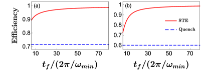
Figure 5: The efficiency relative to the optimal adiabatic result for the short-cut to equilibration (red) and quench (blue) protocols, for (a) expansion protocol, (b) compression protocol.

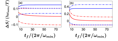
Figure 6: The change in entropy during the (a) expansion and (b) compression processes for the STE (red) and quench (blue) protocols as a function of protocol duration. The change in system entropy $\Delta S_{sys}$, bath entropy $\Delta S_{B}$ and global entropy $\Delta S_{U}$ are indicated by dashed, dashed-dot, and continuous lines respectively.

Appendix E Entropy calculation

The shortcut to equilibration procedure induces a swift change in the system’s entropy $\Delta S_{sys}$. An expansion protocol is accompanied by an increase in the system entropy, while a compression is followed by a decrease in entropy, Figure 6. The STE transforms the system to the target state with high precision, which is almost independent on the protocol duration. As a result, the change in system entropy $\Delta S_{sys}$ also remains constant.

On the contrary, the global entropy generation depends on the trajectory between initial and final states. For large protocol times the STE approaches the adiabatic limit and the global entropy generation $\Delta S_{U}$ vanishes. The heat exchange with the bath increases for shorter protocol duration, which in turn, increases the change in the bath’s entropy, $\Delta S_{B}=-Q_{sys}/T_{B}$. During the expansion (compression) process the system energy decreases (increases), and heat is transferred from (to) the bath, this is accompanied by and decrease (increase) in the bath entropy see Fig. 6.

The change in entropy associated with the quench protocol is composed of a fast isoentropic process, followed by a natural decay towards equilibrium. During the relaxation stage the coherence decays, leading to a rise in the system entropy. For both expansion and compression quench protocols energy flows from the system to the bath, resulting in an increase in the bath entropy and a global entropy production. For both compression and expansion the global irreversible entropy generation of the quench exceeds the STE result.

Appendix F Numerical details

The value of $\omega\left({t}\right)$ is assessed by a numerical solution of equations (10) MP and (4) MP, employing a built in Matlab solver. The solution is used to calculate the system’s evolution according to the inertial solution Dann and Kosloff (2018). The validity of the inertial approximation has been verified, with the inertial parameter obtaining maximum values of $\Upsilon\approx 0.1\,(0.04)$ for the compression (expansion) protocols.
The model parameters are summarized in Table 2.

Table 2:

Coefficient	Value $\left[{\text{atomic units}}\right]$
Oscillator mass	$1$
Compression $\omega\left({0}\right)$	5
Compression $\omega\left({t_{f}}\right)$	10
Expansion $\omega\left({0}\right)$	10
Expansion $\omega\left({t_{f}}\right)$	5
Bath temperature	$2$
Coupling prefactor	$\frac{|\vec{d}|^{2}}{8\pi\varepsilon_{0}\hbar c}=0.02$

References

- Fermi (1956) E. Fermi, Thermodynamics (Dover Publications, 1956).
- Hecht (1990) C. E. Hecht, Statistical thermodynamics and kinetic theory (Freeman, 1990).
- Martínez et al. (2016) I. A. Martínez, A. Petrosyan, D. Guéry-Odelin, E. Trizac, and S. Ciliberto, Nature physics 12, 843 (2016).
- Breuer et al. (2002) H.-P. Breuer, F. Petruccione, et al., The theory of open quantum systems (Oxford University Press on Demand, 2002).
- Alicki (1979) R. Alicki, Journal of Physics A: Mathematical and General 12, L103 (1979).
- Kosloff and Rezek (2017) R. Kosloff and Y. Rezek, Entropy 19, 136 (2017).
- Geva and Kosloff (1992) E. Geva and R. Kosloff, The Journal of chemical physics 96, 3054 (1992).
- Feldmann and Kosloff (2003) T. Feldmann and R. Kosloff, Physical Review E 68, 016101 (2003).
- Dambach et al. (2018) S. Dambach, P. Egetmeyer, J. Ankerhold, and B. Kubala, arXiv preprint arXiv:1806.07700 (2018).
- Verstraete et al. (2009) F. Verstraete, M. M. Wolf, and J. I. Cirac, Nature physics 5, 633 (2009).
- Ye et al. (2008) J. Ye, H. Kimble, and H. Katori, science 320, 1734 (2008).
- Koch (2016) C. P. Koch, Journal of Physics: Condensed Matter 28, 213001 (2016).
- Blaquiere et al. (1987) A. Blaquiere, S. Diner, and G. Lochak, in Proceedings of the 4th International Seminar on Mathematical Theory of Dynamical Systems and Microphysics Udine. Vienna: Springer (Springer, 1987).
- Huang et al. (1983) G. M. Huang, T. J. Tarn, and J. W. Clark, Journal of Mathematical Physics 24, 2608 (1983).
- Brockett et al. (1983) R. W. Brockett, R. S. Millman, and H. J. Sussmann, Progress in mathematics 27, 181 (1983).
- d’Alessandro (2007) D. d’Alessandro, Introduction to quantum control and dynamics (Chapman and Hall/CRC, 2007).
- Brif et al. (2010) C. Brif, R. Chakrabarti, and H. Rabitz, New Journal of Physics 12, 075008 (2010).
- Lloyd and Viola (2000) S. Lloyd and L. Viola, arXiv preprint quant-ph/0008101 (2000).
- Viola et al. (1999) L. Viola, E. Knill, and S. Lloyd, Physical Review Letters 82, 2417 (1999).
- Liu et al. (2011) B.-H. Liu, L. Li, Y.-F. Huang, C.-F. Li, G.-C. Guo, E.-M. Laine, H.-P. Breuer, and J. Piilo, Nature Physics 7, 931 (2011).
- Khodjasteh et al. (2010) K. Khodjasteh, D. A. Lidar, and L. Viola, Physical review letters 104, 090501 (2010).
- Schmidt et al. (2011) R. Schmidt, A. Negretti, J. Ankerhold, T. Calarco, and J. T. Stockburger, Physical review letters 107, 130404 (2011).
- Altafini (2004) C. Altafini, Physical Review A 70, 062321 (2004).
- Vacanti et al. (2014) G. Vacanti, R. Fazio, S. Montangero, G. Palma, M. Paternostro, and V. Vedral, New Journal of Physics 16, 053017 (2014).
- Suri et al. (2017) N. Suri, F. C. Binder, B. Muralidharan, and S. Vinjanampathy, arXiv preprint arXiv:1711.08776 (2017).
- Jing et al. (2013) J. Jing, L.-A. Wu, M. S. Sarandy, and J. G. Muga, Physical Review A 88, 053422 (2013).
- Scandi and Perarnau-Llobet (2018) M. Scandi and M. Perarnau-Llobet, arXiv preprint arXiv:1810.05583 (2018).
- Dann et al. (2018) R. Dann, A. Levy, and R. Kosloff, Phys. Rev. A 98, 052129 (2018).
- Lindblad (1976) G. Lindblad, Communications in Mathematical Physics 48, 119 (1976).
- Gorini et al. (1976) V. Gorini, A. Kossakowski, and E. C. G. Sudarshan, Journal of Mathematical Physics 17, 821 (1976).
- Alicki (2007) R. Alicki, in Quantum Dynamical Semigroups and Applications (Springer, 2007) pp. 1–46.
- Dann and Kosloff (2018) R. Dann and R. Kosloff, arXiv preprint arXiv:1810.12094 (2018).
- Demirplak and Rice (2003) M. Demirplak and S. A. Rice, The Journal of Physical Chemistry A 107, 9937 (2003).
- Berry (2009) M. Berry, Journal of Physics A: Mathematical and Theoretical 42, 365303 (2009).
- Chen et al. (2010) X. Chen, A. Ruschhaupt, S. Schmidt, A. Del Campo, D. Guéry-Odelin, and J. G. Muga, Physical review letters 104, 063002 (2010).
- Muga et al. (2010) J. Muga, X. Chen, S. Ibáñez, I. Lizuain, and A. Ruschhaupt, Journal of Physics B: Atomic, Molecular and Optical Physics 43, 085509 (2010).
- Stefanatos et al. (2010) D. Stefanatos, J. Ruths, and J.-S. Li, Physical Review A 82, 063422 (2010).
- Hoffmann et al. (2011) K. Hoffmann, P. Salamon, Y. Rezek, and R. Kosloff, EPL (Europhysics Letters) 96, 60015 (2011).
- del Campo (2013) A. del Campo, Physical review letters 111, 100502 (2013).
- Torrontegui et al. (2013) E. Torrontegui, S. Ibánez, S. Martínez-Garaot, M. Modugno, A. del Campo, D. Guéry-Odelin, A. Ruschhaupt, X. Chen, and J. G. Muga, in Advances in atomic, molecular, and optical physics, Vol. 62 (Elsevier, 2013) pp. 117–169.
- Abah and Lutz (2017) O. Abah and E. Lutz, arXiv preprint arXiv:1707.09963 (2017).
- Reichle et al. (2006) R. Reichle, D. Leibfried, R. Blakestad, J. Britton, J. D. Jost, E. Knill, C. Langer, R. Ozeri, S. Seidelin, and D. J. Wineland, Fortschritte der Physik: Progress of Physics 54, 666 (2006).
- Isar (2009) A. Isar, Physics of Particles and Nuclei Letters 6, 567 (2009).
- Scutaru (1998) H. Scutaru, Journal of Physics A: Mathematical and General 31, 3659 (1998).
- Banchi et al. (2015) L. Banchi, S. L. Braunstein, and S. Pirandola, Physical review letters 115, 260501 (2015).
- Note (1) Markovianity, as used in this paper, is the condition of timescale separation between a fast decay of the bath correlations and the slow system dynamics.
- Alhassid and Levine (1978) Y. Alhassid and R. Levine, Physical Review A 18, 89 (1978).
- Jaynes (1957) E. T. Jaynes, Physical review 108, 171 (1957).
- Rezek and Kosloff (2006) Y. Rezek and R. Kosloff, New Journal of Physics 8, 83 (2006).
- Andersen et al. (1964) H. Andersen, I. Oppenheim, K. E. Shuler, and G. H. Weiss, Journal of Mathematical Physics 5, 522 (1964).
- Note (2) Namely, the equation is of the Riccati form Hazewinkel (2013); Reid (1972), and an analytical solution in an integral form can be found, once the protocol is defined.
- De Grandi et al. (2010) C. De Grandi, V. Gritsev, and A. Polkovnikov, Physical Review B 81, 012303 (2010).
- Plastina et al. (2014) F. Plastina, A. Alecce, T. Apollaro, G. Falcone, G. Francica, F. Galve, N. L. Gullo, and R. Zambrini, Physical review letters 113, 260601 (2014).
- Chen and Muga (2010) X. Chen and J. G. Muga, Physical Review A 82, 053403 (2010).
- Salamon et al. (2009) P. Salamon, K. H. Hoffmann, Y. Rezek, and R. Kosloff, Physical Chemistry Chemical Physics 11, 1027 (2009).
- Campbell and Deffner (2017) S. Campbell and S. Deffner, Physical review letters 118, 100601 (2017).
- Stefanatos (2017) D. Stefanatos, SIAM Journal on Control and Optimization 55, 1429 (2017).
- Torrontegui et al. (2017) E. Torrontegui, I. Lizuain, S. González-Resines, A. Tobalina, A. Ruschhaupt, R. Kosloff, and J. G. Muga, Phys. Rev. A 96, 022133 (2017).
- Tobalina et al. (2018) A. Tobalina, J. Alonso, and J. G. Muga, New Journal of Physics 20, 065002 (2018).
- Hazewinkel (2013) M. Hazewinkel, Encyclopaedia of Mathematics: Volume 6: Subject Index—Author Index (Springer Science & Business Media, 2013).
- Reid (1972) W. T. Reid, Riccati differential equations (Elsevier, 1972).

References

- Alhassid and Levine (1978) Y. Alhassid and R. Levine, Physical Review A 18, 89 (1978).
- Jaynes (1957) E. T. Jaynes, Physical review 108, 171 (1957).
- Rezek and Kosloff (2006) Y. Rezek and R. Kosloff, New Journal of Physics 8, 83 (2006).
- Dann and Kosloff (2018) R. Dann and R. Kosloff, arXiv preprint arXiv:1810.12094 (2018).
- Kosloff and Rezek (2017) R. Kosloff and Y. Rezek, Entropy 19, 136 (2017).
- Uhlmann (1976) A. Uhlmann, Reports on Mathematical Physics 9, 273 (1976).
- Jozsa (1994) R. Jozsa, J. Mod. Opt. 41, 2315 (1994).
- Marian and Marian (2012) P. Marian and T. A. Marian, Physical Review A 86, 022340 (2012).
- Scutaru (1998) H. Scutaru, Journal of Physics A: Mathematical and General 31, 3659 (1998).
- Isar (2009) A. Isar, Physics of Particles and Nuclei Letters 6, 567 (2009).
- Dann et al. (2018) R. Dann, A. Levy, and R. Kosloff, Phys. Rev. A 98, 052129 (2018).
- Louisell and Louisell (1973) W. H. Louisell and W. H. Louisell, Quantum statistical properties of radiation, Vol. 7 (Wiley New York, 1973).
- Lindblad (1976) G. Lindblad, Reports on Mathematical Physics 10, 393 (1976).
- Breuer et al. (2002) H.-P. Breuer, F. Petruccione, et al., The theory of open quantum systems (Oxford University Press on Demand, 2002).