A new method to probe the mass density and the cosmological constant using configuration entropy

Abstract

We study the evolution of the configuration entropy for different combinations of $\Omega_{m0}$ and $\Omega_{\Lambda 0}$ in the flat $\Lambda$CDM universe and find that the cosmological constant plays a decisive role in controlling the dissipation of the configuration entropy. The configuration entropy dissipates at a slower rate in the models with higher value of $\Omega_{\Lambda 0}$. We find that the entropy rate decays to reach a minimum and then increases with time. The minimum entropy rate occurs at an earlier time for higher value of $\Omega_{\Lambda 0}$. We identify a prominent peak in the derivative of the entropy rate whose location closely coincides with the scale factor corresponding to the transition from matter to $\Lambda$ domination. We find that the peak location is insensitive to the initial conditions and only depends on the values of $\Omega_{m0}$ and $\Omega_{\Lambda 0}$. We propose that measuring the evolution of the configuration entropy in the Universe and identifying the location of the peak in its second derivative would provide a new and robust method to probe the mass density and the cosmological constant.

1 Introduction

Understanding the dark matter and dark energy remain the most challenging problems in cosmology. Observations suggest that the baryons or the ordinary matter constitutes only $\sim 5\%$ of the Universe. It is believed that $\sim\frac{1}{3}$ of the Universe is made up of the gravitating mass out of which $\sim 85\%$ is in the form of a hypothetical unseen matter dubbed as the “dark matter”. The remaining $\sim\frac{2}{3}$ of the Universe is accounted by some mysterious hypothetical component dubbed as the “dark energy”. The dark energy is believed to be responsible for driving the current accelerated expansion of the Universe. The existence and abundance of these mysterious components are determined from various observations.

At present, the $\Lambda$CDM model where $\Lambda$ stands for the cosmological constant and CDM stands for the cold dark matter stands out as the most successful model in explaining most of the cosmological observations till date. The CDM model was initially introduced by Peebles (1982). Davis et al. (1985) carried out the pioneering numerical study of the CDM distribution which paved a new era allowing comparison of theory with multitude of observations.

The current paradigm of structure formation is supported by many complementary observations. The fact that the CMBR angular power spectrum peaks at $l\sim 200$ suggests a spatially flat Universe where the mean energy density of the Universe must be close to the critical density (Komatsu et al., 2011; Planck Collaboration et al., 2016). Other observations from dynamics of galaxies and clusters (Carlberg et al., 1996), the X-ray observations of galaxy clusters (Mohr et al., 1999), Sunyaev-Zeldovich effect (Grego et al., 2000), weak lensing (Benjamin et al., 2007; Fu et al., 2008), baryonic acoustic oscillations (BAO) (Eisenstein et al., 2005), correlation functions (Hawkins et al., 2003) and the power spectrum of density fluctuations (Tegmark et al., 2004; Reid et al., 2010; Percival et al., 2010) revealed that the total mass density parameter including both the baryonic and non-baryonic components must be $\sim 0.3$. A flat Universe with $\Omega_{m}=0.3$ leaves us with no other choice but $\Omega_{\Lambda}=0.7$ which fits the bill perfectly. Further, the existence of dark energy is also supported by independent observations such as Type Ia supernova (Riess et al., 1998; Perlmutter et al., 1999) and BAO (Wang, 2006; Eisenstein, 2005) with very high confidence.

The information entropy can be an useful tool for characterizing the inhomogeneities in the mass distribution (Hosoya et al., 2004; Pandey, 2013). Recently, Pandey (2017) propose that the evolution of configuration entropy of the mass distribution in the Universe may drive the cosmic acceleration. It has been argued that the configuration entropy of the Universe decreases with time due to the amplification of the density perturbations by the process of gravitational instability. The configuration entropy continues to dissipate in a matter dominated Universe. The dissipation of configuration entropy due to this transition from smoother to clumpier state demands existence of some efficient entropy generation mechanisms to counterbalance this loss. If the other entropy generation mechanisms are not sufficient to counter this loss then the Universe must expand in such a way so as to prevent the further growth of structures and stop the leakage of information entropy. Interestingly, the dissipation of the configuration entropy comes to a halt in a $\Lambda$ dominated Universe due to the suppression of the growth of structures on large scales. Recently Das & Pandey (2019) used the evolution of the configuration entropy to distinguish various dynamical dark energy parameterizations. The importance and some interesting implications of inhomogeneities in cosmology has been highlighted earlier in Buchert & Ehlers (1997) and Buchert (2000).

In the present work, we assume that the $\Lambda$CDM model with flat FRW metric to be the correct model of the Universe and the density parameters associated with matter and $\Lambda$ are to be determined from observations. We propose a new method for the determination of the density parameter associated with the mass and the cosmological constant. The method is based on the study of the evolution of the configuration entropy in the Universe. In future, the present generation surveys like SDSS (York et al., 2000), 2dFGRS (Colles et al., 2001), dark energy survey (Abbott et al., 2018) combined with various other future surveys like DESI, Euclid and different future 21 cm experiments like SKA would allow us to measure the configuration entropy at different epochs and study its evolution. The method presented in this work would provide an alternative route to measure the mass density and the cosmological constant in an independent and unique way and compare their values obtained by the other methods from various observations.

2 Theory

2.1 Configuration entropy and its evolution

The observations of the cosmic microwave background radiation (CMBR) suggest that the Universe was highly uniform in the past. But the matter distribution in the present day Universe is highly clumpy due to the structure formation by gravity. Pandey (2017) defines the configuration entropy of the mass distribution following the idea of information entropy (Shannon, 1948) as,

$$S_{c}(t)=-\int\rho(\vec{x},t)\log\rho(\vec{x},t)\,dV.$$ (1)

Here $S_{c}(t)$ is the configuration entropy of the mass distribution at time $t$ over a sufficiently large comoving volume $V$. The volume $V$ is divided into a large number of subvolumes $dV$ and the density $\rho(\vec{x},t)$ is measured inside each volume element.

The distribution is treated as a fluid on large scales. The continuity equation for the fluid in an expanding universe is given by,

$$\frac{\partial\rho}{\partial t}+3\frac{\dot{a}}{a}\rho+\frac{1}{a}\nabla\cdot(\rho\vec{v})=0.$$ (2)

Here $a$ is the scale factor and $\vec{v}$ denotes the peculiar velocity of the fluid inside the volume element $dV$.

If we multiply Equation 2 by $(1+\log\rho)$ and integrate over the entire volume $V$, then we get the entropy evolution equation (Pandey, 2017) as,

$$\frac{dS_{c}(t)}{dt}+3\frac{\dot{a}}{a}S_{c}(t)-\frac{1}{a}\int\rho(3\dot{a}+\nabla\cdot\vec{v})\,dV=0.$$ (3)

Changing variable from $t$ to $a$ in Equation 3 we get,

$$\frac{dS_{c}(a)}{da}\dot{a}+3\frac{\dot{a}}{a}S_{c}(a)-F(a)=0.$$ (4)

where $F(a)$ is given by,

$$F(a)=3MH(a)+\frac{1}{a}\int\rho(\vec{x},a)\nabla\cdot\vec{v}\,dV.$$ (5)

Here $M=\int\rho(\vec{x},a)\,dV=\int\bar{\rho}(1+\delta(\vec{x},a))\,dV$ gives the total mass inside $V$ and $\delta(\vec{x},a)=\frac{\rho(\vec{x},a)-\bar{\rho}}{\bar{\rho}}$ gives the density contrast in a subvolume $dV$ centred at the comoving co-ordinate $\vec{x}$. The $\bar{\rho}$ is the mean density of matter inside the comoving volume $V$.

One can simplify Equation 4 further to get,

$$\frac{dS_{c}(a)}{da}+\frac{3}{a}(S_{c}(a)-M)+\bar{\rho}f(a)\frac{D^{2}(a)}{a}\int\delta^{2}(\vec{x})\,dV=0.$$ (6)

where, $D(a)$ is the growing mode of density perturbation and $f(a)=\frac{dlnD}{dlna}=\frac{a}{D}\frac{dD}{da}$ is the dimensionless linear growth rate.

We need to solve Equation 6 to study the evolution of the configuration entropy for any given cosmological model. The time-independent quantities in the third term of Equation 6 are set to $1$ for the sake of simplicity. We calculate $D(a)$ and $f(a)$ for the cosmological model under consideration. We then numerically solve the Equation 6 using the $4^{th}$ order Runge-Kutta method.

The second and third term in Equation 6 together decides the evolution of the configuration entropy. The second term is decided by the initial condition whereas the third term is governed by the nature of the growth of structures in a particular cosmological model. At the initial stage, the second term solely dictates the evolution because the growth factor remains negligible. The third term only comes into play when the growth of structures becomes significant. So the cosmology dependence of the configuration entropy arises purely from the third term in Equation 6.

The Equation 6 can be solved analytically ignoring the third term which is given by,

$$\frac{S_{c}(a)}{S_{c}(a_{i})}=\frac{M}{S_{c}(a_{i})}+\Bigg{(}1-\frac{M}{S_{c}(a_{i})}\Bigg{)}\Bigg{(}\frac{a_{i}}{a}\Bigg{)}^{3}.$$ (7)

where, $a_{i}$ is the initial scale factor and $S_{c}(a_{i})$ is the initial entropy. We choose $a_{i}$ to be $10^{-3}$ throughout the present analysis. According to this solution, we expect a sudden growth or decay in the configuration entropy near the initial scale factor $a_{i}$ when $S_{c}(a_{i})<M$ and $S_{c}(a_{i})>M$ respectively. On the other hand, no such transients are expected when $S_{c}(a_{i})=M$. Since we are only interested in the cosmology dependence of the configuration entropy, we shall focus on the solution of Equation 6 for $S_{c}(a_{i})=M$ in the present work. The solutions in the other two cases are similar other than the transients present near the initial scale factor.

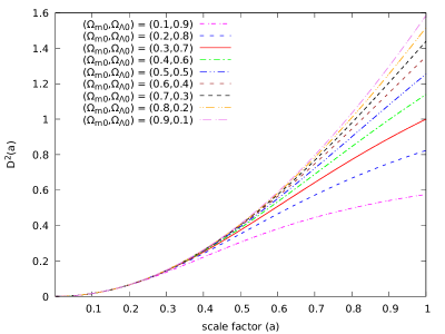
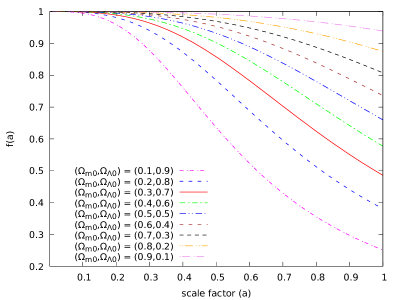
Figure 1: The left panel and the right panel of this figure respectively show $D^{2}(a)$ and $f(a)$ as a function of scale factor for different combinations of $(\Omega_{m0},\Omega_{\Lambda 0})$ within the flat $\Lambda$CDM cosmology. The value of $D(a)$ is normalized to $1$ at present for the combination $(\Omega_{m0},\Omega_{\Lambda 0})=(0.3,0.7)$. The $D(a)$ values in the other models are normalized with respect to this model.

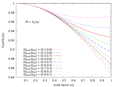
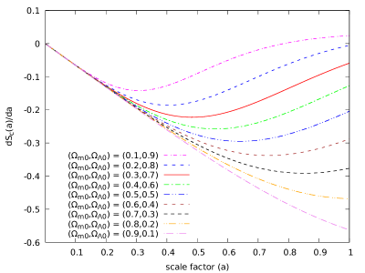
Figure 2: The top left panel of this figure shows the evolution of the configuration entropy for different combinations of $(\Omega_{m0},\Omega_{\Lambda 0})$ within the flat $\Lambda$CDM model. The top right panel and the bottom middle panel respectively show the first and the second derivative of the configuration entropy in these models. The arrows in different colours in the bottom middle panel mark the scale factors $a_{t}=\Big{(}\frac{\Omega_{m0}}{\Omega_{\Lambda 0}}\Big{)}^{\frac{1}{3}}$ corresponding to the transition from matter to $\Lambda$ domination in the respective models. The transition scale factors closely coincide with the peak locations in each model.

2.2 The growing mode and the dimensionless linear growth rate

The CMBR observations show that the Universe is highly isotropic. But the same observations also reveal that there are small anisotropies of the order of $10^{-5}$ imprinted in the CMBR temperature maps. These tiny fluctuations are believed to be the precursor of the large scale structures observed in the present day Universe. The primordial density perturbations were amplified by the process of gravitational instability for billions of years. The growth of the density perturbations $\delta(\vec{x},t)$ can be described by the linear perturbation theory when $\delta<<1$. Considering only perturbations to the matter sector, the linearized equation for the growth of the density perturbation is given by,

$$\frac{\partial^{2}\delta(\vec{x},t)}{\partial t^{2}}+2H\frac{\partial\delta(\vec{x},t)}{\partial t}-\frac{3}{2}\Omega_{m0}H_{0}^{2}\frac{1}{a^{3}}\delta(\vec{x},t)=0.$$ (8)

Here $\Omega_{m0}$ and $H_{0}$ are the present values of the mass density parameter and the Hubble parameter respectively. This equation has two solutions, one which grows and another which decays away with time. The growing mode solution amplifies the density perturbations at the same rate at every location so that the density perturbation at any location $\vec{x}$ can be expressed as, $\delta(\vec{x},t)=D(t)\delta(\vec{x})$. Here $D(t)$ is the growing mode and $\delta(\vec{x})$ is the initial density perturbation at the location $\vec{x}$.

The growing mode solution of Equation 8 can be expressed (Peebles, 1980) as,

$$D(a)=\frac{5}{2}\Omega_{m0}X^{\frac{1}{2}}(a)\int_{0}^{a}\frac{da^{\prime}}{a^{\prime 3}X^{\frac{3}{2}}(a^{\prime})},$$ (9)

where $X(a)=\frac{H(a)^{2}}{H_{0}^{2}}=[\Omega_{m0}a^{-3}+\Omega_{\Lambda 0}]$ in an Universe with only matter and cosmological constant.

In a flat Universe, the dimensionless linear growth rate $f(a)=\frac{d\ln\delta}{d\ln a}$ can be well approximated (Lahav et al., 1991) by,

$$f(a)=\Omega_{m}(a)^{0.6}+\frac{1}{70}[1-\frac{1}{2}\Omega_{m}(a)(1+\Omega_{m}(a))],$$ (10)

where the matter density history $\Omega_{m}(a)$ can be written as $\Omega_{m}(a)=\frac{\Omega_{m0}a^{-3}}{X(a)}$.

In the present work, we consider different combinations of $\Omega_{m0}$ and $\Omega_{\Lambda 0}$ within the framework of the flat $\Lambda$CDM model and calculate $D(a)$ and $f(a)$ in each case. The $D^{2}(a)$ and $f(a)$ for different models are shown in Figure 1. These are then used to solve Equation 6 to study the evolution of the configuration entropy in each model.

3 Results and Conclusions

We show the evolution of $\frac{S_{c}(a)}{S_{c}(a_{i})}$ with scale factor in the top left panel of Figure 2. We see that the configuration entropy initially decreases with time. The dissipation of the configuration entropy is driven by the growth of structures. The dissipation is higher in the models with a larger value of $\Omega_{m0}$. This is directly related to a higher growth factor $D(a)$ and growth rate $f(a)$ in the models with a larger $\Omega_{m0}$ (Figure 1). Clearly, the dissipation is less pronounced in the models with larger $\Omega_{\Lambda 0}$. The structure formation is the outcome of two competing effects: one is the tendency of the overdense regions to collapse under their self gravity and the other is the tendency to move apart with the background expansion. The cosmological constant $\Lambda$ contributes to the later and thus resists the leakage of the configuration entropy in the Universe by increasing the Hubble drag and suppressing the structure formation on large scales.

We show the rate of change of the configuration entropy in the top right panel of Figure 2. We find that the cosmological constant $\Lambda$ plays an influential role in controlling the dissipation of the configuration entropy. Models with larger value of $\Omega_{\Lambda 0}$ and smaller value of $\Omega_{m0}$ show a dip in the slope of the configuration entropy at a smaller value of the scale factor. For example in the model with $\Omega_{\Lambda 0}=0.9$, initially the slope decreases with increasing scale factor reaching the minimum at $a\sim 0.3$. The slope then turns upward remaining negative upto $a\sim 0.8$ thereafter upcrossing the zero. It then slowly plateaus towards a stable value. A similar trend is observed for the other models with different combinations of $\Omega_{m0}$ and $\Omega_{\Lambda 0}$. The minimum occur at $a\sim 0.4$ and $a\sim 0.5$ in the models with $\Omega_{\Lambda 0}=0.8$ and $\Omega_{\Lambda 0}=0.7$ respectively. The minimum of the slope indicates the time since $\Lambda$ becomes proactive in suppressing the dissipation of the configuration entropy. The minimum appears at a smaller value of scale factor in the higher $\Omega_{\Lambda 0}$ models simply because the presence of the $\Lambda$ term is felt earlier in these models.

The bottom middle panel of Figure 2 shows the derivative of the slopes shown in the top right panel of the figure. Initially, the derivative of the slopes are negative for all the models which imply that the slopes are decreasing with time. But the second derivative keeps on increasing with time and eventually upcrosses zero at some value of the scale factor. This scale factor corresponds to the minimum of the slope. For example the model with $\Omega_{\Lambda 0}=0.9$ exhibit the zero upcrossing of the second derivative at $a\sim 0.3$ where a minimum was observed in the slope. Similarly, a zero upcrossing can be seen at $a\sim 0.4$ and $a\sim 0.5$ in the $\Omega_{\Lambda 0}=0.8$ and $\Omega_{\Lambda 0}=0.7$ models respectively. The positive value of the second derivatives after this scale factor suggest that the slopes are increasing with time. However, the slopes themselves remain negative after the occurrence of the minimum. This suggest that the configuration entropy still continues to dissipate with time but with a gradually decreasing rate. The second derivatives of the configuration entropy do not increase monotonically but show a prominent peak at a specific value of the scale factor. The peaks are clearly identified in the models with $\Omega_{\Lambda 0}=0.9$, $\Omega_{\Lambda 0}=0.8$, $\Omega_{\Lambda 0}=0.7$ and $\Omega_{\Lambda 0}=0.6$ at the scale factor $a=0.48$, $a=0.63$, $a=0.75$ and $a=0.87$ respectively. Interestingly, the transition from matter to $\Lambda$ domination in the respective models are expected to occur at nearly the same scale factors. It may be noted that the second derivatives remain negative throughout the entire range of scale factor for $\Omega_{\Lambda 0}=0.1$ and $\Omega_{\Lambda 0}=0.2$ models. The peaks in these models and the rest of the models are expected to occur in future and hence are not present in the figure. The dissipation rate of the configuration entropy changes at a slower rate once the $\Lambda$ domination takes place. This is related to the fact that the growth of structures are completely shut off on larger scales once $\Lambda$ begins to drive the accelerated expansion of the Universe.

We have repeated these analyses for $S_{c}(a_{i})>M$ and $S_{c}(a_{i})<M$ and recovered the peaks at exactly the same locations. This indicates that the peak locations are insensitive to the initial conditions and depend only on the values of $\Omega_{m0}$ and $\Omega_{\Lambda 0}$.

We expect that combining the measurements of the configuration entropy at different redshifts from the present and future generation surveys would enable us to study the evolution of the configuration entropy. This would allow us to identify the location of the peak in its second derivative and constrain the value of both the mass density and the cosmological constant in the Universe.

We would like to point out here that the present method requires us to measure the configuration entropy over a significantly large volume of the Universe. This is to ensure that there are no net mass inflow or outflow across the neighbouring volumes. The present studies suggest that the Universe is homogeneous on large scales (Yadav et al., 2005; Hogg et al., 2005; Sarkar et al., 2009; Sarkar & Pandey, 2016). So at each redshift, a measurement of the configuration entropy over a region extending few hundreds of Mpc would be sufficient for the present analysis. However, the mutual information between the spatially separated but causally connected regions of the Universe may introduce a non-negligible dynamical entanglement between them (Wiegand & Buchert, 2010). Any modification of the evolution equation due to this entanglement need to be investigated further.

Furthermore, the baryonic matter constitutes only a tiny fraction of the matter budget. The baryonic matter distribution is expected to be biased with respect to the dark matter distribution. Currently, the proposed method requires us to map the distribution of an unbiased tracer of the underlying mass distribution at multiple redshifts. The introduction of bias may complicate the analysis which we would like to address in a future work.

Finally, we conclude that the analysis presented in this work provides an alternative avenue for the determination of the mass density and the cosmological constant $\Lambda$ by studying the evolution of the configuration entropy in the Universe. We expect this to find many useful applications in the study of the mysterious dark matter and the elusive cosmological constant.

4 Acknowledgement

The authors thank an anonymous reviewer for valuable comments and suggestions. The authors would like to acknowledge financial support from the SERB, DST, Government of India through the project EMR/2015/001037. BP would also like to acknowledge IUCAA, Pune and CTS, IIT, Kharagpur for providing support through associateship and visitors programme respectively.

References

- Abbott et al. (2018) Abbott, T. M. C., Abdalla, F. B., Allam, S., et al. 2018, ApJS, 239, 18
- Benjamin et al. (2007) Benjamin, J., Heymans, C., Semboloni, E., et al. 2007, MNRAS, 381, 702
- Buchert & Ehlers (1997) Buchert, T., & Ehlers, J. 1997, A&A, 320, 1
- Buchert (2000) Buchert, T. 2000, General Relativity and Gravitation, 32, 105
- Carlberg et al. (1996) Carlberg, R. G., Yee, H. K. C., Ellingson, E., et al. 1996, ApJ, 462, 32
- Colles et al. (2001) Colles, M. et al.(for 2dFGRS team) 2001,MNRAS,328,1039
- Das & Pandey (2019) Das, B., & Pandey, B. 2019, MNRAS, 482, 3219
- Davis et al. (1985) Davis, M., Efstathiou, G., Frenk, C. S., & White, S. D. M. 1985, ApJ, 292, 371
- Eisenstein et al. (2005) Eisenstein, D. J., Zehavi, I., Hogg, D. W., et al. 2005, ApJ, 633, 560
- Eisenstein (2005) Eisenstein, D. J. 2005, New Astronomy Reviews, 49, 360
- Fu et al. (2008) Fu, L., Semboloni, E., Hoekstra, H., et al. 2008, A&A, 479, 9
- Grego et al. (2000) Grego, L., Carlstrom, J. E., Joy, M. K., et al. 2000, ApJ, 539, 39
- Hawkins et al. (2003) Hawkins, E., Maddox, S., Cole, S., et al. 2003, MNRAS, 346, 78
- Hogg et al. (2005) Hogg, D. W., Eisenstein, D. J., Blanton, M. R., Bahcall, N. A., Brinkmann, J., Gunn, J. E., & Schneider, D. P. 2005, ApJ, 624, 54
- Hosoya et al. (2004) Hosoya, A., Buchert, T., & Morita, M. 2004, Physical Review Letters, 92, 141302
- Komatsu et al. (2011) Komatsu, E., Smith, K. M., Dunkley, J., et al. 2011, ApJS, 192, 18
- Lahav et al. (1991) Lahav, O., Lilje, P. B., Primack, J. R., & Rees, M. J. 1991, MNRAS, 251, 128
- Mohr et al. (1999) Mohr, J. J., Mathiesen, B., & Evrard, A. E. 1999, ApJ, 517, 627
- Pandey (2013) Pandey, B. 2013, MNRAS, 430, 3376
- Pandey (2017) Pandey, B. 2017, MNRAS, 471, L77
- Peebles (1980) Peebles, P. J. E. 1980, The Large-scale Structure of the Universe, Princeton University Press, 1980. 435 p.,
- Peebles (1982) Peebles, P.J. E. 1982, ApJ, 263, L1
- Percival et al. (2010) Percival, W. J., Reid, B. A., Eisenstein, D. J., et al. 2010, MNRAS, 401, 2148
- Perlmutter et al. (1999) Perlmutter, S., Aldering, G., Goldhaber, G., et al. 1999, ApJ, 517, 565
- Planck Collaboration et al. (2016) Planck Collaboration, Ade, P. A. R., Aghanim, N., et al. 2016, A&A, 594, A13
- Reid et al. (2010) Reid, B. A., Percival, W. J., Eisenstein, D. J., et al. 2010, MNRAS, 404, 60
- Riess et al. (1998) Riess, A. G., Filippenko, A. V., Challis, P., et al. 1998, AJ, 116, 1009
- Sarkar et al. (2009) Sarkar, P., Yadav, J., Pandey, B., & Bharadwaj, S. 2009, MNRAS, 399, L128
- Sarkar & Pandey (2016) Sarkar, S., & Pandey, B. 2016, MNRAS, 463, L12
- Shannon (1948) Shannon, C. E. 1948, Bell System Technical Journal, 27, 379-423, 623-656
- Tegmark et al. (2004) Tegmark, M., Blanton, M. R., Strauss, M. A., et al. 2004, ApJ, 606, 702
- Wang (2006) Wang, Y. 2006, ApJ, 647, 1
- Wiegand & Buchert (2010) Wiegand, A., & Buchert, T. 2010, Physical Review D, 82, 023523
- Yadav et al. (2005) Yadav, J., Bharadwaj, S., Pandey, B., & Seshadri, T. R. 2005, MNRAS, 364, 601
- York et al. (2000) York, D. G., et al. 2000, AJ, 120, 1579