Effect of particle exchange on the glass transition of binary hard spheres

Abstract

We investigate the replica theory of the liquid-glass transition for a binary mixture of large and small additive hard spheres. We consider two different ansätze for this problem: the frozen glass ansatz (FGA) in whichs the exchange of large and small particles in a glass state is prohibited, and the exchange glass ansatz (EGA), in which it is allowed. We calculate the dynamical and thermodynamical glass transition points with the two ansätze. We show that the dynamical transition density of the FGA is lower than that of the EGA, while the thermodynamical transition density of the FGA is higher than that of the EGA. We discuss the algorithmic implications of these results for the density-dependence of the relaxation time of supercooled liquids. We particularly emphasize the difference between the standard Monte Carlo and swap Monte Carlo algorithms. Furthermore, we discuss the importance of particle exchange for estimating the configurational entropy.

1 Introduction

The relaxation time of supercooled liquids increases dramatically upon decreasing temperature or increasing density, and eventually exceeds the experimentally accessible time scale, giving rise to the glass transition [1, 2]. Despite decades of studies, the underlying mechanisms that cause the glass transition have yet to be fully understood. One of the biggest problems is how to define a proper order parameter for the transition, because a typical configuration of the glass is essentially as random as a standard liquid at slightly higher temperatures. The replica liquid theory (RLT) considers $m$ replicas of the original system in order to circumvent the problem [3, 4]. In the liquid phase, the $m$ replicas move independently, while in the glass phase, the $m$ replicas are confined around their center of mass and behave like a molecule [5, 6]. Thus, one can use the correlation function of the $m$ replicas as a thermodynamic order parameter, which physically corresponds to the long-time limit of the time correlation of a single replica in the glass phase.

The RLT was first developed for one-component systems [5, 7] and later extended to binary mixtures [8, 9, 10]. In the latter case, the simplest ansatz corresponds to assuming that all replicas in a molecule are of the same species. From the physical point of view, this assumption is tantamount to prohibit the exchange of particles in a glass state [8, 10], which we hereafter refer to as the frozen glass ansatz (FGA). However, the FGA-RLT displays unphysical behavior in the one-component limit [8]. The entropy of the glass, as predicted by the FGA, remains larger than that of the one-component system by the mixing entropy,

$$s_{\rm mix}=-\sum_{\mu}x_{\mu}\log x_{\mu}\ ,$$ (1)

where $N_{\mu}$ is the number of particles of the $\mu$-th species, $N=\sum_{\mu}N_{\mu}$, and $x_{\mu}=N_{\mu}/N$, even in the limit where all particles are identical.

Figure 1: Schematic examples of configurations of the $m=2$ replicated system. The number of the first (red) and second (blue) species are $N_{1}=12$ and $N_{2}=8$, respectively. The purple circles denote particles of either species. (Left) A configuration of the one-component system. The configuration does not change under the exchange of any pair of particles, and the Gibbs factor is $(N_{1}+N_{2})!$. (Middle) A configuration of the FGA. The configuration is only invariant under the exchange of molecules of the same species. The Gibbs factor is then $N_{1}!N_{2}!$. (Right) A configuration of the EGA. The Gibbs factor is the same as that of the one-component system, $G=(N_{1}+N_{2})!$.

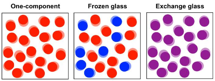
As discussed by Coluzzi et al. [8], the above discrepancy originates from the Gibbs factor of the replicated system, i.e. the number of exchanges of molecules that leave the configuration of the system invariant. In Fig. 1, we show the schematic configuration of a replicated system for $m=2$, $N_{1}=12$ and $N_{2}=8$. For one-component systems, all molecules are identical, and the Gibbs factor is $G=(N_{1}+N_{2})!$. For binary mixtures, if one assumes the FGA, only the molecules of the same species can be exchanged, leading to the Gibbs factor $G=N_{1}!N_{2}!$, and to an entropy difference $\Delta S=-\Delta\log G=\log(N_{1}+N_{2})!-\log(N_{1}!N_{2}!)=Ns_{\rm mix}$ with respect to the one-component system. Note that $\Delta S$ only depends on the particle numbers, and it thus remains constant even in the one-component limit.

To resolve this contradiction, one should allow the exchange of replicas of different species (i.e. the dissociation of molecules), see the right panel in Fig. 1. In this case, the particle species in a molecule change with time. After averaging over the time, the molecules are indistinguishable, meaning that the Gibbs factor is $G=(N_{1}+N_{2})!$, and the one-component result is recovered. Hereafter, we shall refer to this as the exchange glass ansatz (EGA). From the physical point of view, the EGA is tantamount to allow the exchange of particles in a glass state; the exchange process leads to the dissociation of molecules. Note that the FGA corresponds to the extreme case of the EGA when the probability of exchanging particles of different species vanish. This is indeed the case if, say, the size ratio of different species is sufficiently large. On the contrary, if the size ratio is close to unity or particles have a continuous size distribution, the EGA is needed to avoid unphysical behavior.

The difference between the FGA and EGA also sheds light into the algorithmic dependence of the relaxation time of supercooled liquids [11, 12] (see [13] for an alternative approach). Recently, it has been shown that the swap Monte Carlo (SMC) algorithm, which is nothing but a standard Monte Carlo algorithm (MC) combined with particle exchange moves, significantly accelerates the relaxation of supercooled liquids [14, 15]. The FGA and EGA give an effective description, within mean field theory, of the metastable states accessible by MC and SMC [11]. Over a time scale sufficiently shorter than the relaxation time $\tau_{\alpha}$, particles undergo vibrational motion around their equilibrium position. The exchange of particle species hardly occurs over this time scale in standard MC, meaning that the FGA gives a good description of the corresponding metastable state. On the contrary, the SMC exchanges the particle species as well as the particle positions. Particle exchanges thus frequently occur even at time scales shorter than $\tau_{\alpha}$, meaning that the corresponding metastable state would be well described by the EGA. It is expected that the FGA and EGA give different glass transition points, which provides an explanation for the difference of relaxation time between the standard MC and SMC [11, 12].

An explicit implementation of the EGA has been provided quite recently in Ref. [16]. In previous work [11], we applied the formalism of Ref. [16] to the Mari-Kurchan model [17], a mean field model of the glass transition of binary hard spheres. In this work, we apply the formalism to a more realistic model, i.e. binary hard spheres in three dimensions, which allows us to calculate quantitatively the values of dynamical and thermodynamical quantities.

The organization of the paper is as follows. In Section 2, we briefly summarize the mean field scenario of the glass transition, on which the RLT relies. In Section 3, we introduce the model. In Section 4, we extend the RLT to binary mixtures, particularly emphasizing the way to take into account particle exchange. In Sections 5 and 6, we discuss the results and conclude the work.

2 A mean field theory of glass transition

Here, we briefly summarize the random first order transition (RFOT) theory, which is a semi-phenomenological theory of the glass transition built on the analogy with a class of mean field spin-glasses [18, 19]. The key assumption of RFOT theory is that the slow dynamics around the glass transition is due to the emergence of complex structures within the free-energy landscape. The ROFT theory predicts that the dynamics of supercooled liquids changes qualitatively around two important points. The first is the dynamical transition, at packing fraction $\varphi_{d}$, at which long-lived metastable states appear in the free energy landscape. Mean field theories of the glass transition, such as the mode-coupling theory (MCT), predict that the relaxation time diverges as $\tau_{\alpha}\sim(\varphi_{d}-\varphi)^{-\gamma}$ [20, 21]. In finite dimensions, however, because of the thermal fluctuations, the system escape from a metastable state after a sufficiently long time. The activation events are driven by the configurational entropy $\Sigma(\varphi)$, which is the logarithm of the number of metastable states [18, 19]. The second important point is the Kauzmann transition, at packing fraction $\varphi_{K}$, at which $\Sigma(\varphi)$ vanishes. For $\varphi>\varphi_{K}$, the system is permanently stuck in a free energy minimum, because it can no longer acquire entropy by visiting several other minima. In this regime, the system is referred to as an ideal glass, and it has a finite rigidity [22]. Below, we calculate the transition points $\varphi_{d}$ and $\varphi_{K}$, as well as the configurational entropy $\Sigma(\varphi)$, of binary hard spheres by using the RLT.

3 Model

We now introduce the model used in this work. We consider a binary mixture of large and small particles. The total interaction potential is

$$V_{N}=\sum_{i<j}^{1,N}v_{\mu_{i}\mu_{j}}(x_{i}-x_{j})\ ,$$ (2)

where $x_{i}$ denotes the position of the $i$-th particle, and $\mu_{i}\in\{\rm Large,\ Small\}$ denotes the particle species. We use the additive hard sphere potential:

$$v_{\mu\nu}(r)=\left\{\begin{array}[]{ll}\infty&r<\frac{\sigma_{\mu}+\sigma_{\nu}}{2}\\ 0&r\geq\frac{\sigma_{\mu}+\sigma_{\nu}}{2}\end{array}\right.,$$ (3)

where $\sigma_{\rm Large}$ and $\sigma_{\rm Small}$ denote the radius of large and small particles, respectively. The total number of particles is $N$, and the volume of the system is $V$. For hard spheres, the temperature $T$ does not affect thermodynamic quantities [23]. The relevant control parameters are the packing fraction $\varphi=V^{-1}\sum_{i=1}^{N}\frac{4\pi\sigma_{\mu_{i}}^{3}}{3}$, the size ratio $r=\sigma_{\rm Large}/\sigma_{\rm Small}$, and the fraction of the species $x_{\rm Large}=N_{\rm Large}/N$ or $x_{\rm Small}=1-x_{\rm Large}$.

4 Derivation of the RLT equations

Here, we derive the RLT equations for binary hard spheres. For this purpose, we extend the quantitative approximation scheme that has been developed in [24] for one-component hard spheres.

4.1 Effective potential method

Our starting point is the replicated partition function [5, 6, 16]

$$Z_{m}=\sum_{N=0}^{\infty}\frac{1}{N!}\left(\prod_{a=1}^{m}\prod_{i=1}^{N}\sum_{\mu^{a}_{i}}\int dx_{i}^{a}\right)e^{-\beta\sum_{a=1}^{m}\sum_{i<j}^{1,N}v_{\mu_{i}\mu_{j}}(x_{i}^{a}-x_{j}^{a})+\sum_{i=1}^{N}\psi_{\overline{\mu}_{i}}(\overline{x}_{i})},$$ (4)

where $\overline{x}_{i}=\{x_{i}^{1},\cdots,x_{i}^{m}\}$ and $\overline{\mu}_{i}=\{\mu_{i}^{1},\cdots,\mu_{i}^{m}\}$ denote the position and species of the $i$-th particle in the replica space. $\psi$ is the chemical potential conjugated to the one point replicated density distribution,

$$\rho_{\overline{\mu}}(\overline{x})=\sum_{i=1}^{N}\left\langle{\prod_{a=1}^{m}\delta(x^{a}-x_{i}^{a})\delta_{\mu^{a}\mu_{i}^{a}}}\right\rangle=\frac{\delta\log Z_{m}}{\delta\psi_{\overline{\mu}}(\overline{x})}\ ,$$ (5)

which is directly related to the order parameter. For instance, the cage size $A$ is given by

$$A =\sum_{\overline{\mu}}\int d\overline{x}\rho_{\overline{\mu}}(\overline{x})(x^{a}-x^{b})^{2}\ ,$$ (6)

for an arbitrary pair $ab$. In order to determine $\rho_{\overline{\mu}}(\overline{x})$, one first performs a Legendre transformation, which expresses the free energy as a functional of $\rho_{\overline{\mu}}(\overline{x})$, and then optimizes the transformed free energy w.r.t $\rho_{\overline{\mu}}(\overline{x})$. For the calculation of the replicated free energy, we use the effective potential method, which allows us to map the replicated system onto a non-replicated system, by integrating out the degree of freedom of $m-1$ replicas [6]. Let us choose the first replica $a=1$ as a reference. The effective potential of the first replica is

$$e^{-\beta v^{\rm eff}_{\mu^{1}\nu^{1}}(x^{1}-y^{1})} =\frac{1}{x_{\mu_{1}}x_{\nu_{1}}}e^{-\beta v_{\mu^{1}\nu^{1}}(x^{1}-y^{1})}\left(\prod_{a=2}^{m}\sum_{\mu^{a}\nu^{a}}\int dx^{a}dy^{a}\right)\times$$ (7)

$$\times\rho_{\overline{\mu}}(\overline{x})\rho_{\overline{\nu}}(\overline{y})e^{-\beta\sum_{a=2}^{m}v_{\mu^{a}\nu^{a}}(x^{a}-y^{a})}$$

$$=e^{-m\beta v_{\mu^{1}\nu^{1}}(x^{1}-y^{1})}\left(1+Q_{\mu^{1}\nu^{1}}(x^{1}-y^{1})\right),$$

where

$$Q_{\mu^{1}\nu^{1}}(x^{1}-y^{1}) =-1+\frac{e^{-(1-m)\beta v_{\mu^{1}\nu^{1}}(x^{1}-y^{1})}}{x_{\mu}^{1}x_{\nu}^{1}}\times$$ (8)

$$\times\left(\prod_{a=2}^{m}\sum_{\mu^{a}\nu^{a}}\int dx^{a}dy^{a}\right)\rho_{\overline{\mu}}(\overline{x})\rho_{\overline{\nu}}(\overline{y})e^{-\beta\sum_{a=2}^{m}v_{\mu^{a}\nu^{a}}(x^{a}-y^{a})}\ .$$

We approximate the replicated free energy by the free energy of the first replica, interacting with the effective potential defined in Eq. (7),

$$-\beta F_{m}=\log Z_{m}\approx\Delta S_{\rm vib}-m\beta F[v^{\rm eff}]\ ,$$ (9)

where $\Delta S_{\rm vib}$ is the additional vibrational entropy coming from the other $m-1$ replicas in the ideal gas term,

$$\Delta S_{\rm vib}=\sum_{\overline{\mu}}\int d\overline{x}\rho_{\overline{\mu}}(\overline{x})(1-\log\rho_{\overline{\mu}}(\overline{x}))-N\sum_{\mu}x_{\mu}(1-\log\rho_{\mu})\ .$$ (10)

In a glass state, the $m$ replicas undergo vibrational motion around their center of mass, suggesting that $Q_{\mu^{1}\nu^{1}}$ can be considered as a small perturbation. Expanding Eq. (9) for small $Q_{\mu^{1}\nu^{1}}$, we obtain

$$-\beta F_{m} \approx\Delta S_{\rm vib}-m\beta F(T^{*})+\frac{1}{2}\sum_{\mu\nu}\rho_{\mu}\rho_{\nu}\int dxdyg_{\mu\nu}(x,y)Q_{\mu\nu}(x-y)\ ,$$ (11)

where $\rho_{\mu}=x_{\mu}\rho$, $\rho=N/V$, $F(T^{*})$ denotes the free energy of the non-replicated liquid with the bare potential, at the effective temperature $T^{*}=T/m$, and $g_{\mu\nu}(x,y)$ denotes its pair correlation function. Finally, we replace the bare potential in $Q_{\mu\nu}$ as $e^{-\beta v_{\mu\nu}(r)}\to g_{\mu\nu}(r)^{1/m}$, which has been shown to significantly improve the accuracy of the approximation in the one-component system case [24].

Full optimization of the free energy for completely general $\rho_{\overline{\mu}}(\overline{x})$ is very difficult. To simplify this calculation, we approximate $\rho_{\overline{\mu}}(\overline{x})$ as

$$\rho_{\overline{\mu}}(\overline{x})\approx\rho(\overline{x})g(\overline{\mu})\ ,$$ (12)

where

$$\rho(\overline{x})=\sum_{i}\left\langle{\prod_{a}\delta(x^{a}-x_{i}^{a})}\right\rangle\ ,\qquad g(\overline{\mu})=\frac{1}{N}\sum_{i}\left\langle{\prod_{a}\delta_{\mu^{a}\mu_{i}^{a}}}\right\rangle.$$ (13)

In principle, this assumption can be relaxed, but the calculation becomes very involved [11]. For the positional degrees of freedom, we assume the standard Gaussian ansatz [5, 6]:

$$\rho(\overline{x})=\rho\int dX\prod_{a=1}^{m}\gamma_{A}(x^{a}-X)\ ,\qquad\gamma_{A}(r)=\frac{e^{-r^{2}/2A}}{(2\pi A)^{d/2}}\ ,$$ (14)

which implies that the cage vibrations of the $m$ replicas follow the Gaussian distribution around their center of mass $X$. The remaining task, which we shall discuss in the following subsections, is to formulate an ansatz for $g(\overline{\mu})$.

4.2 Frozen Glass Ansatz (FGA)

If the size ratio $r$ is sufficiently large, particles of different species cannot be exchanged in a glass state. This frozen situation is described by a simple ansatz, in which each molecule of the replicated system consists of particles of the same species, as illustrated in the middle panel in Fig. 1. More concretely, we assume

$$g(\overline{\mu})=\sum_{\mu}x_{\mu}\prod_{a=1}^{m}\delta_{\mu\mu^{a}}.$$ (15)

Substituting this into the vibrational entropy, Eq. (10), one obtains

$$\frac{\Delta S_{\rm vib}}{N}=\frac{d}{2}(m-1)[1+\log(2\pi A)]+\frac{d}{2}\log m-(m-1)\sum_{\mu}x_{\mu}\log x_{\mu}\ .$$ (16)

Also, Eq. (8) reduces to

$$Q_{\mu\nu}(r) =-1+g_{\mu\nu}(r)^{(1-m)/m}\int dr^{\prime}\gamma_{2A}(r+r^{\prime})q_{\mu\nu}(r^{\prime})^{m-1},$$

$$q_{\mu\nu}(r) =\int dr^{\prime}\gamma_{2A}(r+r^{\prime})g_{\mu\nu}(r)^{1/m}\ .$$ (17)

The equilibrium value of the cage size $A$ is obtained from the saddle point condition $\left.\partial_{A}\log Z_{m}\right|_{m=1}=0$. Substituting Eq. (17) into Eq. (11), one gets

$$A=M(A),$$ (18)

where

$$M(A)=\left[-\frac{\rho}{d}\sum_{\mu\nu}x_{\mu}x_{\nu}\int dr\frac{\partial q_{\mu\nu}(r)}{\partial A}\log q_{\mu\nu}(r)\right]^{-1}.$$ (19)

The configurational entropy $\Sigma$ is calculated by using the Monasson’s formula [3]:

$$\Sigma=\lim_{m\to 1}m^{2}\frac{\partial}{\partial m}\left(\frac{\beta F_{m}/N}{m}\right).$$ (20)

Using above equation, it is straightforward to show that

$$\Sigma =s_{\rm liq}-\frac{d}{2}\log(2\pi A)-d$$ (21)

$$-\frac{\rho}{2}\sum_{\mu\nu}x_{\mu}x_{\nu}\int dr\left[q_{\mu\nu}(r)\log q_{\mu\nu}(r)-g_{\mu\nu}(r)\log g_{\mu\nu}(r)\right]\ ,$$

where $s_{\rm liq}$ is the entropy per particle of the bare liquid at temperature $T^{*}$. In the one-component limit, $r\to 1$, the FGA gives a pathological result. In this limit, the interaction term converges to the one-component result $-\frac{\rho}{2}\int dr\left[q(r)\log q(r)-g(r)\log(r)\right]$, while the liquid entropy becomes $s_{\rm liq}=s_{\rm liq}^{\rm one}+s_{\rm mix}$. Thus, the difference between $\Sigma$ of the one-component and two-component systems does not vanish, $\Delta\Sigma\to s_{\rm mix}>0$. This unphysical behavior implies that the FGA must break down around $r\sim 1$. In the next section, we show that this problem can be cured by taking into account particle exchange.

4.3 Exchange Glass Ansatz (EGA)

Figure 2: Dependence of the order parameter for particle exchange, $q(\Delta)$, on the coupling $\Delta$.

Here we derive the free energy within an ansatz that takes into account the effect of particle exchange in a glass state. For this purpose, we first map the particle species to a binary spin variable by introducing $\sigma(\mu)$, where $\sigma(\rm Large)=1$ and $\sigma(\rm Small)=-1$. We assume that $\sigma(\mu)$ follows the same distribution as a mean field spin glass model [25, 11],

$$g(\overline{\mu}) =C_{m}(\Delta)^{-1}e^{H\sum_{a=1}^{m}\sigma(\mu^{a})+\frac{\Delta^{2}}{2}\sum_{ab}^{1,m}\sigma(\mu^{a})\sigma(\mu^{b})}$$ (22)

$$=C_{m}(\Delta)^{-1}\int Dhe^{(h+H)\sum_{a=1}^{m}\sigma(\mu^{a})},$$

where

$$Dh=dh\frac{1}{\sqrt{2\pi\Delta^{2}}}e^{-\frac{h^{2}}{2\Delta^{2}}}\ ,$$ (23)

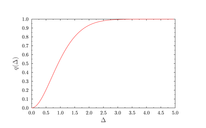
and $C_{m}(\Delta)=\int Dh\left(\sum_{\mu}e^{(h+H)\sigma(\mu)}\right)^{m}$ is the normalization constant. The value of $H$ fixes the species concentration $x_{\mu}$, which is calculated as $x_{\mu}=\sum_{\overline{\mu}}g(\overline{\mu})\delta(\mu^{a},\mu)$. To simplify the calculation, hereafter we consider the equimolal binary mixture with $x_{L}=x_{S}=1/2$, which corresponds to $H=0$. The value of $\Delta$ controls the correlation of the particle species among different replicas,

$$q(\Delta) \equiv\lim_{m\to 1}\frac{2}{m(m-1)}\sum_{a<b}\left\langle{\sigma(\mu^{a})\sigma(\mu^{b})}\right\rangle$$ (24)

$$=\lim_{m\to 1}\sum_{\overline{\mu}}\int d\overline{x}\rho_{\overline{\mu}}(\overline{x})\sigma(\mu^{1})\sigma(\mu^{2})$$

$$=C_{1}(\Delta)^{-1}\int Dh2\cosh(h)\tanh(h)^{2}.$$

In Fig. 2, we show that $q(\Delta)$ is a monotonically increasing function of $\Delta$. The value $q=0$ corresponds to completely uncorrelated species in a molecule, while the value $q=1$ corresponds to molecules of identical species, i.e. to the FGA.

Substituting Eq. (22) into Eq. (10), one can calculate the vibrational entropy as

$$\frac{\Delta S_{\rm vib}}{N} =\frac{d}{2}(m-1)\log(2\pi A)+\frac{d}{2}(m-1+\log m)+\log C_{m}(\Delta)$$ (25)

$$-\frac{\Delta^{2}}{2}(m+m(m-1)q_{m}(\Delta))+\sum_{\mu}x_{\mu}\log x_{\mu}.$$

Similarly, Eq. (8) reduces to

$$Q_{\mu\nu}(r) =-1+g_{\mu\nu}(r)^{(1-m)/m}\frac{1}{x_{\mu}x_{\nu}}\int\frac{DuDv}{C_{m}^{2}}e^{u\sigma(\mu)+v\sigma(\nu)}$$ (26)

$$\times\int dr^{\prime}\gamma_{2A}(r+r^{\prime})q(r,u,v)^{m-1}\ ,$$

where $Du,Dv$ are defined in Eq. (23) and

$$q(r,u,v)=\sum_{\mu\nu}e^{u\sigma(\mu)+v\sigma(\nu)}\int dr^{\prime}\gamma_{2A}(r+r^{\prime})g_{\mu\nu}(r^{\prime})^{1/m}\ .$$ (27)

Substituting Eqs. (25) and (26) into Eq. (11), we obtain the replicated free energy. One can derive the self-consistent equations for $A$ and $\Delta$ from the extremization condition $\partial_{A}\log Z_{m}=\partial_{\Delta}\log Z_{m}=0$. Because the derivation is straightforward, but the result is cumbersome, we do not show the explicit expressions here. Using the Monasson’s formula, Eq. (20), we obtain the configurational entropy as

$$\Sigma =s_{\rm liq}-\frac{d}{2}\log(2\pi A)-d-\frac{f(\Delta)}{2}+\frac{\Delta^{2}}{2}(1+q(\Delta))$$ (28)

$$-\frac{\rho}{2}\int dr\Bigg{\{}\frac{e^{-\Delta^{2}}}{4}\int DuDvq(r,u,v)\left[\log q(r,u,v)-f(\Delta)\right]$$

$$-\sum_{\mu\nu}x_{\mu}x_{\nu}g_{\mu\nu}(r)\log g_{\mu\nu}(r)\Bigg{\}}\ ,$$

where we have introduced an auxiliary function:

$$f(\Delta)\equiv\lim_{m\to 1}\frac{2}{C_{m}(\Delta)}\frac{\partial C_{m}(\Delta)}{\partial m}=e^{-\frac{\Delta^{2}}{2}}\int Dh\,2\cosh(h)\log(2\cosh(h))\ .$$ (29)

In the one-component limit, $r\to 1$, one can show that $\Delta\to 0$ and $-f(\Delta)/2\to-\log(2)=-s_{\rm mix}$, which exactly cancels out the mixing entropy in $s_{\rm liq}$. Thus, we recover the configurational entropy of the one-component system obtained in previous work [24]:

$$\Sigma\to s_{\rm liq}^{\rm one}-\frac{d}{2}\log(2\pi A)-d-\frac{\rho}{2}\int dr\left[q(r)\log q(r)-g(r)\log g(r)\right].$$ (30)

4.4 Numerics

Here we summarize how to calculate $A$ and $\Delta$ numerically for a given $\varphi$ and $r$. Our theory requires the liquid entropy per particle $s_{\rm liq}$ and the pair correlation function $g_{\mu\nu}(r)$ as input. Following previous work [9, 24], we use a binary version of the Carnahan-Starling (CS) approximation [26] for $s_{\rm liq}$, and the Verlet-Weis approximation [27] for $g_{\mu\nu}(r)$, see A for details. To solve the self-consistent equations for $A$ and $\Delta$, we first set $A=A_{\rm ini}$ and $\Delta=\Delta_{\rm ini}$ for the initial conditions, where we selected $A_{\rm ini}=10^{-3}$ and $\Delta_{\rm ini}=10^{-1}$ (and we confirmed that the final results are independent of this choice if $A_{\rm ini}$ and $\Delta_{\rm ini}$ are sufficiently small). Then, we solve the self-consistent equations using a standard iterative method. When $\varphi<\varphi_{d}$, this iterative process does not converge, which indicates that $A\to\infty$. In practice, we stop the calculation when $A$ exceeds unity during the iteration process. When $\varphi>\varphi_{d}$, $A$ and $\Delta$ converge to finite values. In this case, we stop the calculation when $\left|{(A_{i+1}-A_{i})/A_{i}}\right|<10^{-10}$. By substituting $\Delta$ into Eq. (24), one gets the correlation $q(\Delta)$ of particle species.

5 Results

In this section, we present numerical results for the order parameters, $A$ and $q(\Delta)$, and the configurational entropy $\Sigma$.

5.1 Order parameter

Figure 3: Dependence of the order parameters on packing fration $\varphi$. (Top) The cage size $A$. The results of the FGA and EGA are shown with blue and red markers, respectively. The dashed and full vertical lines indicate the dynamical and Kauzmann transition points, respectively. (Bottom) The correlation of particle species $q$ calculated with the EGA.

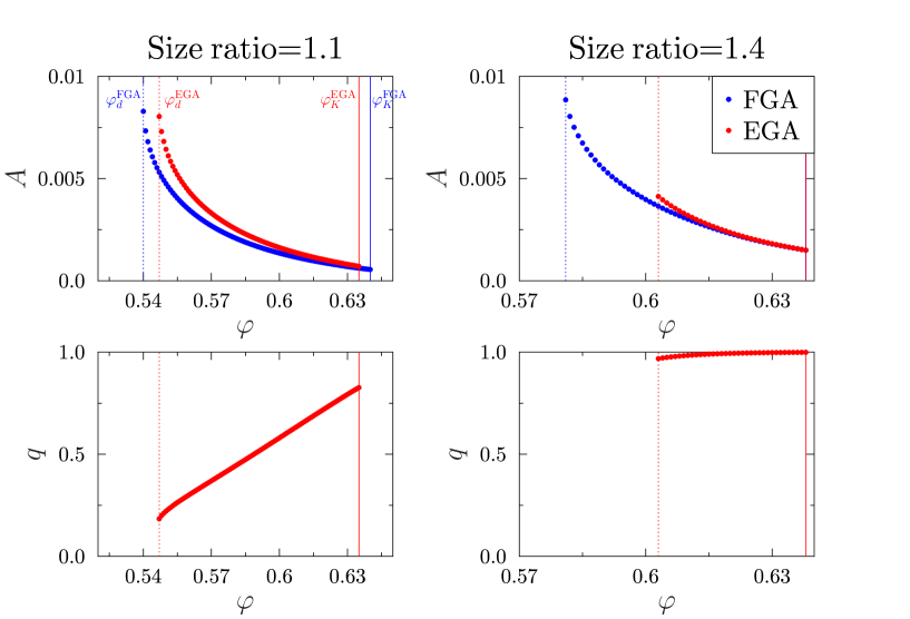
In Fig. 3, we show the numerical results for $A$ and $q(\Delta)$ for size ratios $r=1.1$ and $r=1.4$. For $r=1.1$ (left panels in Fig. 3), for sufficiently small $\varphi$, $A=\infty$ and $q=0$, meaning that there is no correlation between different replicas, and the system behaves as a standard liquid. $A$ and $q$ begin to have finite values at packing fraction $\varphi=\varphi_{d}$, corresponding to the dynamical transition. The dynamical transition point of the FGA is smaller than that of the EGA, $\varphi_{d}^{\rm FGA}<\varphi_{d}^{\rm EGA}$. As mentioned in the introduction, this might explain the efficiency of the SMC reported in recent numerical simulations [15], if one identifies $\varphi_{d}^{\rm FGA}$ and $\varphi_{d}^{\rm EGA}$ as the dynamical transition points of the standard MC and SMC, respectively [11]. For the same $\varphi$, the value of $A$ calculated with the FGA is smaller than that of the EGA, which is also consistent with numerical results [15]. Above $\varphi_{d}^{\rm EGA}$, $q$ increases with $\varphi$. This is a natural result, because particle exchanges hardly occur at high $\varphi$. For very high $\varphi$, the effect of particle exchange is negligible, and the values of $A$ calculated with the FGA and EGA are similar. The difference between $\varphi_{d}^{\rm FGA}$ and $\varphi_{d}^{\rm EGA}$ increases with increasing $r$ (right panels in Fig. 3). Above $\varphi_{d}^{\rm EGA}$, the FGA and EGA give very similar values of $A$, which is consistent with the higher value of $q$ above $\varphi_{d}^{\rm EGA}$.

5.2 Configurational entropy

We calculate the configurational entropy $\Sigma$ by substituting the order parameters calculated in the previous section into Eqs. (21) and (28). $\Sigma$ is well defined only for $\varphi>\varphi_{d}$, because otherwise the order parameters do not have finite values, indicating that there are no metastable states.

Figure 4: Dependence of the configurational entropy $\Sigma$ on packing fraction $\varphi$, for size ratio $r=1.1$ (left) and $r=1.4$ (right). The blue and red markers indicate the results of the FGA and EGA, respectively.

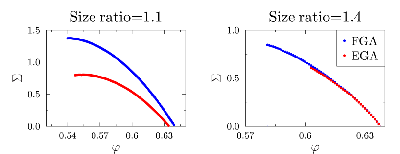
In Fig. 4, we show the numerical results for small and large size ratios, $r=1.1$ and $r=1.4$. For $r=1.1$, the complexity calculated with the FGA has a higher value than that calculated with the EGA. This results can be naturally understood as follows. The complexity is the difference between the entropies of the liquid and the (metastable) glass, $\Sigma=s_{\rm liquid}-s_{\rm glass}$. In general, $s_{\rm glass}$ calculated with the EGA is larger than with the FGA, since the EGA includes extra degree of freedom (the species) in the glass description. As a consequence, the EGA predicts a lower value of $\Sigma$. The Kauzmann transition point, $\varphi_{K}$, is defined by $\Sigma(\varphi_{K})=0$. Due to the higher value of $\Sigma$, the FGA predicts a higher value of the Kauzmann transition with respect to the EGA, $\varphi_{K}^{\rm FGA}>\varphi_{K}^{\rm EGA}$. A similar trend is observed for the larger size ratio $r=1.4$, see the right panel in Fig. 4. The difference of $\Sigma$ calculated with the FGA and EGA decreases with increasing $r$, simply because large and small particle are hardly exchanged.

5.3 Phase diagram

In Fig. 5, we show the phase diagram predicted by our theory.

Figure 5: Phase diagram of equimolar binary hard spheres in three dimensions. Blue and red symbols represent the results of the FGA and EGA, respectively. Circles represent the dynamical transition point $\varphi_{d}$, while squares represent the Kauzmann transition $\varphi_{K}$. The solid lines are guides to the eye.

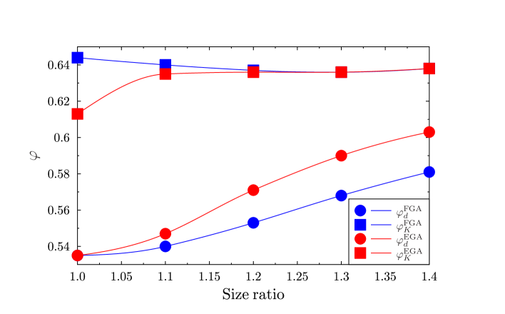
We first discuss the dynamical transition points $\varphi_{d}^{\rm FGA}$ and $\varphi_{d}^{\rm EGA}$. For $r>1$, we always obtain $\varphi_{d}^{\rm FGA}<\varphi_{d}^{\rm EGA}$. This is consistent with recent results from mode coupling theory (MCT) [12]. However, MCT predicts that $\varphi_{d}^{\rm FGA}$ is almost independent of $r$, while our theory predicts that $\varphi_{d}^{\rm FGA}$ monotonically increases with $r$. This discrepancy may come from the approximation made in Eq. (12), where we assumed that the cage size $A$ does not depend on the species. In principle one can avoid this approximation and construct a more accurate theory, but the calculation gets much harder [11]. We leave this investigation for future work.

The behavior of the Kauzmann transition points, $\varphi_{K}^{\rm FGA}$ and $\varphi_{K}^{\rm EGA}$, is qualitatively different from that of $\varphi_{d}^{\rm FGA}$ and $\varphi_{d}^{\rm EGA}$. We observe that $\varphi_{K}^{\rm FGA}>\varphi_{K}^{\rm EGA}$ for all $r$, which is a consequence of the behavior of the configurational entropy $\Sigma$ described in Sec.5.2. The difference between $\varphi_{K}^{\rm FGA}$ and $\varphi_{K}^{\rm EGA}$ decreases with increasing $r$. This is a natural result because large and small particle are hardly exchanged for large $r$, and in particular at high density near $\varphi_{K}$. We would like to stress that the FGA is metastable with respect to the EGA, because the EGA is a more general ansatz within a variational theory. This means that the thermodynamically meaningful transition point is not $\varphi_{K}^{\rm FGA}$ but $\varphi_{K}^{\rm EGA}$. One should then take into account the degrees of freedom associated to particle exchange when calculating the entropy of the glass state, otherwise the Kauzmann transition point is overestimated. A numerical algorithm for this purpose has been recently proposed in [28].

6 Summary and discussions

In this work, we theoretically investigated a binary hard sphere mixture by using the replica liquid theory (RLT). For this purpose, we constructed two different ansätze: the frozen glass ansatz (FGA), where the replicas in similar position are constrained to be of the same species, and the exchange glass ansatz (EGA), where the replicas in similar position can have different species. Using these ansätze, we calculated the transition points for different size ratio $r$. We found that the dynamical transition point calculated using the FGA is smaller than that of the EGA, $\varphi_{d}^{\rm FGA}<\varphi_{d}^{\rm EGA}$. The opposite relation holds for the Kauzmann transition point, $\varphi_{K}^{\rm FGA}>\varphi_{K}^{\rm EGA}$. In the rest of this section, we discuss possible implications of our results for experimental and numerical studies of the glass transition.

As mentioned in the introduction, our theoretical results might give insight on the increased efficiency of the swap Monte Carlo algorithm (SMC), as compared to the standard Monte Carlo algorithm (MC) [15, 29]. For this discussion, it is useful to introduce two timescales: the density relaxation time, $\tau_{\alpha}$, and the typical timescale to exchange large and small particles in a metastable glass state, $\tau_{\rm ex}$. Over a time scale sufficiently shorter than the relaxation time, $t\ll\tau_{\alpha}$, the system is trapped in a metastable state where particles just undergo vibrational motion. In case of MC, large and　 small particles are hardly exchanged in this timescale, implying that $\tau_{\rm ex}\gg\tau_{\alpha}$, thus the effect of the particle exchange is negligible. The metastable state is then well described by the FGA. On the contrary, using the SMC with $r$ close enough to unity, large and small particles are easily exchanged, implying that $\tau_{\rm ex}\ll\tau_{\alpha}$. In this case, the EGA provides a good description of the metastable state. Within these assumptions, the efficiency of the SMC is explained by the larger value of $\varphi_{d}^{\rm EGA}$ with respect to $\varphi_{d}^{\rm FGA}$. Note that it is known that the SMC works only for binary mixtures of sufficiently small size ratio $r\approx 1.2$ [14] or continuous polydisperse system [15]. For binary mixtures of large size ratio $r\approx 1.4$, the SMC gives a compatible result with that of the MC [28]. This cannot be explained by our phase diagram, Fig. 5, where the difference between $\varphi_{d}^{\rm EGA}$ and $\varphi_{d}^{\rm FGA}$ does not vanish even around $r\approx 1.4$. The same result is also obtained by MCT [12]. The inefficiency of SMC at large $r$ should instead be attributed to the fact that the assumption $\tau_{\rm ex}<\tau_{\alpha}$ does not hold for larger $r$, even for the SMC, because the exchange moves are never accepted. The EGA thus no longer gives a good description of the metastable state. Unfortunately, because $\tau_{\rm ex}$ is a purely dynamical quantity, it cannot be calculated by a static theory such as the RLT. It would be interesting to extend dynamical theories of the glass transition, such as the mode-coupling theory (MCT), to calculate $\tau_{\rm ex}$ and reconcile this discrepancy between theoretical and numerical results.

Appendix A Verlet-Weis approximation for binary mixtures

Here we review the binary version of the Verlet-Weis (VW) approximation. We label here the two species by indices $i,j\in\{1,2\}$. As for a one-component system, we assume that $g_{ij}(r)$ can be written as

$$g_{ij}^{\rm VW}(r)=\theta(r-\sigma_{ij})\left[g^{\rm PY}(\xi r)+\Delta g_{ij}(r)\right],$$

$$\xi=\left(\frac{\varphi}{\varphi^{*}}\right)^{1/3},$$

$$\varphi^{*}=\varphi-\frac{\varphi^{2}}{16}\ ,$$

$$\Delta g_{ij}(r)=\frac{A_{ij}}{r}e^{-b_{ij}(r-\sigma_{ij})}\cos(b_{ij}(r-\sigma_{ij}))\ ,$$ (31)

where

$$A_{ij}/\sigma_{ij}=g_{ij}^{\rm CS}(\sigma_{ij})-g_{ij}^{\rm PY}(\xi\sigma_{ij},\varphi^{*})\ ,$$ (32)

where $g_{ij}^{\rm CS}$ and $g_{ij}^{\rm PY}$ denote the results of the Carnahan-Starling approximation (CS) [26] and Percus-Yevick approximation (PY) [30], respectively. We determine $b_{ij}$ from the consistency of the compressibility equations:

$$\frac{\partial\beta P^{\rm CS}}{\partial\rho} =1-\sum_{ij}x_{i}x_{j}\rho\int d\bm{r}c_{ij}^{\rm VW}(\bm{r})=\sum_{ij}\left[\delta_{ij}-\rho_{i}c_{ij}^{\rm VW}(k=0)\right]x_{j}$$ (33)

$$=\sum_{ij}\left[\bm{I}+\bm{H}(0)\right]_{ij}^{-1}x_{j}=\sum_{ij}x_{i}x_{j}S_{ij}^{-1}(0)\ .$$

where

$$\left[\bm{I}+\bm{H}(k)\right]_{ij} =\delta_{ij}+\rho_{i}h_{ij}(k)\ ,$$

$$S_{ij}(k) =\delta_{ij}x_{j}+\rho x_{i}x_{j}h_{ij}(k)\ .$$ (34)

Here, $S_{ij}(k)$ denotes the structural factor and $h_{ij}(k)$ denotes the Fourier transform of the pair correlation function. For a binary mixture, we have

$$S_{11}^{-1} =\frac{1}{D}\left(x_{2}+\rho x_{2}^{2}h_{22}\right)\ ,$$

$$S_{12}^{-1} =S_{21}^{-1}=-\frac{1}{D}\rho x_{1}x_{2}h_{12}\ ,$$

$$S_{22}^{-1} =\frac{1}{D}\left(x_{1}+\rho x_{1}^{2}h_{11}\right)\ ,$$ (35)

where

$$D =(x_{1}+\rho x_{1}^{2}h_{11})(x_{2}+\rho x_{2}^{2}h_{22})-x_{1}^{2}x_{2}^{2}h_{12}.$$ (36)

At large $\varphi$, the compressibility has a large value, which implies that

$$\lim_{k\to 0}D(k) =\lim_{k\to 0}(x_{1}+\rho x_{1}^{2}h_{11}(k))(x_{2}+\rho x_{2}^{2}h_{22}(k))-x_{1}^{2}x_{2}^{2}h_{12}(k)\approx 0.$$ (37)

We shall determine the value of $b_{ij}$ from this condition. First, note that $h_{ij}(k)$ can be decomposed as

$$h_{ij}(k) =\int dre^{ikr}\left[g_{ij}(r)-1\right]=h_{ij}^{\rm PY}(k)+\Delta h_{ij}(k)\ ,$$

$$h_{ij}^{\rm PY}(k) =\int dre^{ikr}\left[\theta(r-\sigma_{ij}/\xi)g_{ij}^{\rm PY}(\xi r)-1\right]\ ,$$

$$\Delta h_{ij}(k) =\int dre^{ikr}\left[\theta(r-\sigma_{ij})-\theta(r-\sigma_{ij}/\xi)\right]g^{\rm PY}(\xi r)$$ (38)

$$+\int dre^{ikr}\theta(r-\sigma_{ij})\Delta g_{ij}(r)\ .$$

Substituting the above equations into Eq. (37), we have

$$D(0) =D^{\rm PY}(0)+O(\Delta h_{ij}(0)).$$ (39)

Because $D(0)$ and $D^{\rm PY}(0)$ are expected to have small values, $O(\Delta h_{ij})$ terms should also vanish. The simplest condition is then

$$\Delta h_{ij}(0) =0\ .$$ (40)

This condition can be solved for $b_{ij}$, leading to

$$b_{ij} =\frac{24A_{ij}}{\sigma_{ij}^{2}\varphi g^{\rm PY}(\sigma_{ij},\varphi^{*})}\approx\frac{24A_{ij}}{\sigma_{ij}^{2}\varphi^{*}g^{\rm PY}(\sigma_{ij},\varphi^{*})}\ .$$ (41)

References

- [1] Debenedetti P G and Stillinger F H 2001 Nature 410 259
- [2] Cavagna A 2009 Physics Reports 476 51–124
- [3] Monasson R 1995 Phys. Lev. Lett. 75 2847
- [4] Franz S and Parisi G 1995 Journal de Physique I 5 1401–1415
- [5] Mézard M and Parisi G 1999 J. Phys. Condens. Matter 11 A157
- [6] Parisi G and Zamponi F 2010 Rev. Mode. Phys. 82 789
- [7] Parisi G and Zamponi F 2005 J. Chem. Phys. 123 144501
- [8] Coluzzi B, Mézard M, Parisi G and Verrocchio P 1999 J. Chem. Phys. 111 9039–9052
- [9] Biazzo I, Caltagirone F, Parisi G and Zamponi F 2009 Phys. Lev. Lett. 102 195701
- [10] Ikeda H, Miyzaki K, Yoshino H and Ikeda A 2017 arXiv:1710.08373
- [11] Ikeda H, Zamponi F and Ikeda A 2017 J. Chem. Phys. 147 234506
- [12] Szamel G 2018 Phys. Rev. E 98(5) 050601
- [13] Wyart M and Cates M E 2017 Phys. Rev. Lett. 119(19) 195501
- [14] Grigera T S and Parisi G 2001 Phys. Rev. E 63(4) 045102
- [15] Ninarello A, Berthier L and Coslovich D 2017 Phys. Rev. X 7(2) 021039
- [16] Ikeda H, Miyazaki K and Ikeda A 2016 J. Chem. Phys. 145 216101
- [17] Mari R and Kurchan J 2011 J. Chem. Phys. 135 124504
- [18] Kirkpatrick T, Thirumalai D and Wolynes P G 1989 Phys. Rev. A 40 1045
- [19] Bouchaud J P and Biroli G 2004 J. Chem. Phys. 121 7347–7354
- [20] Bengtzelius U, Gotze W and Sjolander A 1984 J. Phys. Condens. Matter 17 5915
- [21] Götze W 2008 Complex dynamics of glass-forming liquids: A mode-coupling theory vol 143 (OUP Oxford)
- [22] Yoshino H and Mézard M 2010 Phys. Rev. Lett. 105(1) 015504
- [23] Hansen J P and McDonald I R 1990 Theory of simple liquids (Elsevier)
- [24] Mangeat M and Zamponi F 2016 Phys. Rev.E 93 012609
- [25] Mézard M, Parisi G and Virasoro M 1987 Spin glass theory and beyond: An Introduction to the Replica Method and Its Applications vol 9 (World Scientific Publishing Company)
- [26] Santos A, López de Haro M and Yuste S 2005 J. Chem. Phys. 122 024514
- [27] Verlet L and Weis J J 1972 Mol. Phys. 24 1013–1024
- [28] Ozawa M, Parisi G and Berthier L 2018 arXiv:1805.06017
- [29] Berthier L, Charbonneau P, Coslovich D, Ninarello A, Ozawa M and Yaida S 2017 PNAS 201706860
- [30] Lebowitz J 1964 Phys. Rev. 133 A895