Ultraviolet activity as indicators of small-scale magnetic fields in $\gamma$ Cassiopeiae

Abstract

The recorded activity of $\gamma$ Cas (B0.5 IVe) in the ultraviolet is important to an understanding of the mechanism behind this prototypical Be star’s high energy activity, especially its hard X-ray emissions. Our analysis focuses first on the phasing of ultraviolet and optical light curves from different epochs. The rotational interpretation of the 1.22 d optical signal is justified in part on this phasing. Next we detail observations of “migrating subfeatures,” which traverse blue to red across line profiles in high quality spectra. These are likely to be proxies for surface magnetic fields, which have not been detected yet by spectropolarimetric means in rapid rotating Be stars like $\gamma$ Cas. We also analyze the important responses of the semi-forbidden resonance S IV line at $\lambda$1404.8 to simultaneous X-ray variations. These results offer indirect support for the existence of small-scale magnetic fields on this Be star.

1 Introduction

$\gamma$ Cas is the prototypical member of the class of “classical Be stars” (Rivinius et al., 2013) and also the prototype of a subgroup of some 22 stars that exhibit copious hard X-ray flux (Nazé & Motch, 2018). These fluxes are variable on timescales from a few seconds to a year or longer - for a review see Smith et al. (2016, “SLM16”). Stars of this subgroup are evolved on the main sequence and are confined to a spectral type range of about O9.7-B1.5. We will adopt the following parameters for $\gamma$ Cas: an age of at least 20 Myr, a spectral type of B0.5 IVe, a mass of $\simeq$13-15 M_⊙, a radius of about 10 R_⊙, and a ${\rm v\,sin\,i}$ $\approx$ 441 km s^-1 (Frémat et al., 2005). We view its decretion disk and presumably the star at an inclination of 42${\pm 4}^{\circ}$ (Stee et al., 2012). The last parameters indicate that the star’s rotation rate is near the critical velocity, a fact also deduced from its ${\rm v\,sin\,i}$ being at the upper limit observed for early Be stars (Motch et al., 2015, “M15”). We estimate combined errors for the radius and ${\rm v\,sin\,i}$ as $\pm{20\%}$. Our inference concerning critical rotation is also consistent with the star’s periodic photometric signature (with P_rot = 1.21 d; 0.822 cy d^-1) found from long-term $V$ and $B$ band monitoring with an Automated Photometric Telescope (APT) system (Henry & Smith, 2012, “HS12”). This signal had disappeared by 2012 or 2013.

$\gamma$ Cas is is in a 203.6 d binary with a near-circular orbit (Nemravová et al., 2012; Smith et al., 2012). The companion has a mass of 0.9${\pm 0.4}$ M_⊙. The fact that the secondary’s UV flux is $<$0.6% of the total for the system (Wang et al., 2017) demonstrates that any variations in UV spectra, such as discussed below, cannot originate from this companion or a disk surrounding it. Also, although its evolutionary status is otherwise unknown, the UV limit does rule out the secondary’s being an sdOB star.

Two general explanations have been put forth for the emission of the peculiar hard X-ray emission from this class of variables. The first is that stellar wind or disk wind particles accrete onto a degenerate secondary, such as a neutron star (“NS”; White et al., 1982; Postnov et al., 2017) or white dwarf (“WD” Murakami et al., 1986; Hamaguchi et al., 2016) and convert their liberated potential energy to X-rays. Tsujimoto et al. (2018) have contrasted the expected phenomenalogies for the magnetic and nonmagnetic cases, under the assumption of accretion onto some type of WD secondary.

The second scenario, to which we confine ourself herein and for which the current status of the secondary star is unimportant, is the “magnetic star-disk interaction picture” (Smith & Robinson, 1999; Robinson & Smith, 2000; Robinson et al., 2002, “SR99, RS00, RSH”). In this picture small-scale fields emerging from the Be star entangle with a toroidal disk field and reconnect. As they do so, they accelerate electron beams onto the Be star’s surface, where they produce the ubiquitous, rapid quasi-flares and background “basal” flux we observe. Because internal fossil magnetic fields in early B stars are unlikely to be at work, a key question in the magnetic interaction picture is: where do the putative surface fields come from?

To address this question, M15 pointed to the prediction by Cantiello et al. (Cantiello et al., 2009; Cantiello & Braithwaite, 2011a; Cantiello et al., 2011b, “CB11a”) that the revised Fe opacities cause a thin equatorial convection zone to be set up in rapidly rotating massive stars such as $\gamma$ Cas.  They predicted that nonpermanent circulations are driven in these zones that produce so-called $\sigma\omega$ dynamos and local magnetic fields. Field lines drift to the surface where they emerge. The interaction picture extends this idea by positing the entanglement of these fields with the disk’s, with the ensuing release of X-rays.

This paper is based on an integrated analysis done for all the correlations observed in $\gamma$ Cas between X-ray variations and those in the UV and optical domains. This approach has led to the extension of facts not comprehensively put together to date. These include: (1) persistent variations in the UV and optical light curves around the rotational period and long-cycles observed in the X-ray and optical regimes (RSH) and (2) the “migrating subfeatures” in optical and UV line profiles (SR99). We develop these points now so as to facilitate planning of optical, X-ray and, in the long-term, UV observations.

2 Early reports of multi-wavelength correlations in $\gamma$ Cas

To recount the history of multi-wavelength correlations discovered in $\gamma$ Cas, it is important to include what was observed before recent generations of UV and X-ray satellites. The first reports were based on a simultaneous campaign in 1977 undertaken with the Copernicus satellite (Slettebak & Snow, 1978; Peters, 1982). Let us recall that Copernicus was able to observe targets in the UV and medium X-ray at the same time.

Using the Copernicus X-ray camera, Peters (1982) found a rapid X-ray “burst” on 1977 January 27.95; this burst was confirmed by Polidan (1994) and Parmar (1994). At the same time, the Copernicus UV scanners, V1 and U1, slowly scanned the Mg II and Si IV resonance doublets, respectively. One V1 scan disclosed brief emissions in the red wings of both Mg II lines. Simultaneously, the U1 scanner slowly traversed the Si IV doublet. When it reached $\lambda$1394 it revealed emission in this line’s red wing, just as in the Mg II lines. While these observations were in progress, Slettebak & Snow obtained a series of ground-based H$\alpha$ spectra and discovered a five-sigma emission “flare” in this line.

Other flare-like events have been occasionally observed in $\gamma$ Cas.  Similar to the 1978 burst of Peters, Murakami et al. (1986) discovered a several minute X-ray “flare” occurring on 1983 October 31, a circumstance probably due to a confluence of a few smaller events (Smith et al., 1998a, “SRC”). In the optical, Smith (1995) discovered a “flare” appearing in the red wing of He I $\lambda$6678, just five minutes after a spectrum that exhibited no feature. Three minutes after the “flare” appeared, another spectrum showed that the feature had already weakened but was still visible. The feature did not reappear in subsequent spectra of the observing night. A cosmic ray event as a false signal could be ruled out.

All these events occurred quickly, lasting only minutes.

3 Recent multi-wavelength correlations

Such unexpected events as these were the impetus for a simultaneous campaign on $\gamma$ Cas organized by SRC on 1996 March 14-15 using the Rossi X-ray Timing Explorer (RXTE) and the Goddard High Resolution Spectrograph (GHRS), attached to the Hubble Space Telescope. These observations lasted 27 hr and 21.3 hr, respectively. The GHRS spectra were centered on the $\lambda$1394, $\lambda$1403 complex and covered a total of 36 Ångstroms. Most of the discussion in this paper will not focus on the behavior of this doublet.

3.1 Correspondences in UV and optical time series

3.1.1 UV light curves with repeating features

To add to the GHRS spectra, we consulted the International Ultraviolet Explorer (IUE) archives to search for high-dispersion, short-wavelength spectral time series with dense sampling over at least a full rotational period. The archives disclose two such records, one in 1982 January and the other in 1996 January. Their durations were 44 hr and 33 hr, respectively.

Fluxes for wavelengths bins at the blue and red ends of the GHRS spectra were coadded to determine a quasi-continuum flux. This step was repeated for each spectrum in the time series to determine a “UVC” light curve. We similarly cobinned IUE Short Wavelength Prime camera fluxes in the echelle orders covering $\lambda\lambda$1200-1260 (except for the Ly$\alpha$ order) to obtain the corresponding IUE-based light curves. The GHRS curve, originally displayed by Smith et al. (1998b, “SRH”), is plotted as the top curve in Figure 1. This curve is rendered with a small offset in the ordinate for visual clarity. A similar offset was applied to the 1996 January dataset. Since the SRH paper was published the rotational period of $\gamma$ Cas has been redetermined by the APT optical light curve monitoring over 15 years (Smith et al., 2006a, “SHV”) and HS12. These studies resulted in a period P_rot = 1.215811 $\pm{0.000030}$ d. A recent reanalysis of the APT dataset has shown that the derived period has a weak dependence on how the prewhitening is performed against a stronger 70-80 d cycle signal. In fact the derived value would be a few $\sigma$ larger if no prewhitening were to be applied to the data (Henry, 2018). In the work described just below we derived a slightly revised value, P^′_rot = 1.21585 d, from the alignment in phase of optical and UVC features in Fig. 1. This value lies just outside the formal $\pm{1\sigma}$ limit given by SHV and HS12. Herein we adopt this revised value.

Figure 1: The coalignment of the UV dips in the three GHRS and IUE light curves of $\gamma$ Cas,  based on P^′_rot = 1.21585 d. The true dips are shown in bold or as large symbols. The significances of statistically false fluctuations (in range of dotted line) in the IUE curves are $\leq$2$\sigma$, while the actual dips in the lower curve are 3.8$\sigma$ and 4.0$\sigma$, respectively. The horizontal bar at top denotes the phase range of the broad “bright star” optical maximum of the ephemeris of Henry & Smith (2012) when period-folded with P^′_rot.

The GHRS light curve of $\gamma$ Cas of Fig. 1 exhibits two principal “dip” features of amplitude $\approx$1% and $\approx$2%, respectively, separated in time by 9.6${\pm 0.5}$ hr. SRH noted that two extended IUE light curves of this star showed similar features. SRH normalized the UVC echelle fluxes from spectra SWP16127-16193 to create the 1996 January 27-29 UVC curve. We have since improved this normalization slightly by dividing the far-UV echelle fluxes by sums from four long-wavelength echelle orders ($m$ = 68-71) instead of just one. Although the differences in the relative fluxes for this curve in Fig. 1, relative to their original depiction by SRH, are barely noticeable, they do serve to better define the noise in flux from the judged nonvariable stretch of fluxes in the time series. Note that we dropped the first spectrum of the 1982 series because the stellar image was not well centered in the spectrograph entrance aperture.

In Fig. 1 we have aligned the pairs of dips in the three UVC curves that were used to compute the revised P^′_rot value. The statistical significances of putative dips in the two IUE curves shown in the plot were tested by a computer routine, ewcalc.pro, the author wrote to assess equivalent width differences from IUE spectra using many Monte Carlo realizations, i.e. by first assessing r.m.s. noise in the data and then seeing how many simulations are required to match the total observed flux excursions from the nominal level (Smith et al., 2006b). The results of this exercise indicate that a total of three small fluctuations before time $\approx$6 hr are not statistically significant. However, the two dips in the range “7-23 hr” appearing in the 1996 January dataset are just significant, at 3.8${\pm 0.5}$$\sigma$ and 4.0${\pm 0.5}$$\sigma$.

The 1996 IUE light curve was not optimal in that the instrument had to be turned off for what could have been three observations during times “10-13 hr,” while the satellite entered the South Atlantic Anomaly (SAA) zone. This duration coincided with the predicted time of the first dip, according to the GHRS record. A similar, though less obtrusive, SAA gap occurred during the appearance of the same dip feature in the 1982 light curve. Notice that the first and second dips in the 1996 January IUE UVC curve may have been similar in strength, in contrast to their relative sizes in the GHRS curve 57 days earlier. Yet, the first dip was the dominant feature in the 1982 curve, and one rotation cycle later at $\approx$40 hr it reappeared much weaker. In all, although nominal thermodynamic parameters for the absorbing, moderate-sized, “clouds” responsible for these dips were published by SRH, it must be kept in mind that they, or parameters from some anisotropic geometry, may not have unambiguous or constant values.

3.1.2 Bright star optical phase vis à vis UVC light curves

SH12’s folded optical light curve for $\gamma$ Cas (their Fig. 8) exhibits a broad “bright-star” plateau. In order to match this waveform at different epochs, we computed the ephemeris of this feature using the period P^′_rot and a fiducial $T_{\rm o}$ (computed at Reduced Julian Date = 53000.41 d) for the faint star phase. Thus, in Fig. 1 the horizontal bar depicts the phasing of this plateau, with error bars, during the 1996 March campaign. In our picture at these times, lasting $\sim$$\frac{1}{3}$ of a rotational cycle, an observer will witness two major activity centers on opposite limbs of the Be star. In the moderately precise APT photometry the centers will appear unresolved as one bright plateau. For the precise UV GHRS dataset they will appear as two distinct, but shallow, minima.

3.1.3 The flux curve of S IV $\lambda$1404.8

In Figure 2 we overplot the 1996 March 14-15 RXTE/X-ray 16 s fluxes and its derived smoothed curve (dots and dashes, respectively) and GHRS/UVC light curve original data (fuzzy dashes). The latter has been flipped and rescaled to match the extrema of the smoothed RXTE curve. As the two curves are almost indistinguishable, the correlation between them is excellent. (Note that the full extent or quality of extended X-ray-UV correlations applies at other epochs is not established on the bais of this campaign alone.)

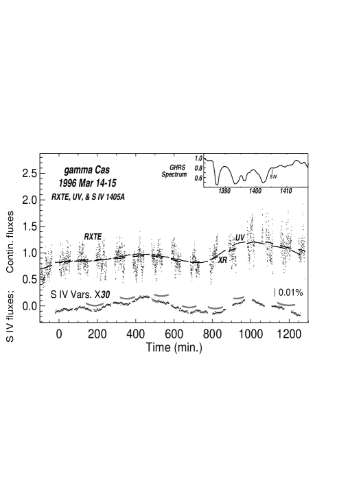
Figure 2: Upper curves in main panel: the RXTE 16 s (dots) and smoothed data overplotted with the inverted UVC continuum light curve. The UV data have small r.m.s. errors and appear here as a fuzzy dashed line. The lower curve shows fluxes extracted from the Si IV $\lambda$1404.8 line. The added upward-convex arcs above this curve indicate the times during which migrating subfeatures are seen in Si IV line grayscale. The top inset shows the position of this S IV line in the spectrum.

SLM16 discussed correlations in the flux curves extracted from Fe V, Si IV, and Si III lines in the GHRS spectra in a similar manner to the UVC curve shown in Fig. 1. They noted that the Fe V curve was well anti-correlated with the RXTE curve, even as the silicon line curves were similarly directly correlated with it. They pointed out that this could best be explained by a shift in ionization of the UV-emitting gas in response to increased X-ray emission from a nearby X-ray source(s), thus spatially linking the UV-emitting medium to this source. An alternative explanation due to the introduction of absorption columns (like those producing the two UVC dips) does not serve, since most of these UV lines exhibit decreased absorption during these times.

The inset of Fig. 2 depicts the S IV $\lambda$1404.8 line in the GHRS spectrum. This line is the strongest member of a weak resonance multiplet, of which $\lambda$1406.0 is the next strongest. Since these transitions are also semi-forbidden, their log gf values are some four orders of magnitudes below those of other lines in the spectrum (including the Si IV doublet). Thus they probe further into the intervening bodies responsible for the UVC dips. The S IV extraction curve shown exhibits a tight scatter. Once again the correlation with X-ray flux is excellent.

3.2 Spectral migrating subfeatures

Next we visit an important spectral feature that emerges from the “grayscale” of the GHRS time series - the grayscale is formed from subtracting the mean spectrum from each spectrum of the time series. The result is a two dimensional representation of temporal variations. The grayscale of our 1996 campaign (see Fig. 8 of SLM16) displays prominent gray striations running across spectral lines. These have become known as “migrating subfeatures.”

Migrating subfeatures (msf) are a pattern of blue-to-red absorption features traversing across the centers of optical and/or UV line profiles in two known groups of stars: $\gamma$ Cas (and perhaps HD 110432; see Smith & Balona (2006, “SB”)) as one group, and a large group of cool, magnetically-active stars of which AB Dor is the prototype. The msf phenomenon was first discovered by Robinson & Collier Cameron (1986) and ascribed to “prominences” forced into corotation by surface magnetic fields. These structures are situated typically 1-2 corotation radii above the star (Collier Cameron & Robinson, 1989a, b, “CCRa, CCRb6”). Spectropolarimetry has confirmed the presence of multipolar fields on the surface of AB Dor (Donati et al., 2003). The spectra of many stars in this “AB Dor class” suggests that a complex magnetic topology is a common attribute in this group (e.g., Dunstone et al., 2006; Stauffer et al., 2017).

Msf were first discovered in optical line profiles of $\gamma$ Cas by Yang et al. (1988) and also observed in ground-based spectra described by Smith (1995). As implied above, the best sampled observations of them were obtained from the GHRS spectra from the 1996 campaign. The msf were found to show an acceleration of +95 km^-1hr^-1. Also, they were associated mainly with lines of less excited ions, e.g., they are typically visible in S IV and Si III but not Fe V lines. One difference from the msf of AB Dor spectra is that they are quite short-lived (1 to 1-$\frac{1}{2}$ hr). Also, the underlying activity cells are likely to be brighter than the surrounding stellar surface (CB11a). This fact allows them to appear more easily as spectral absorption features.

For the present study we have probed deeper than SR99 and examined the fainter response of the $\lambda$1406 line as well as the stronger member. We ran new exoatmospheric CIRCUS models similar to those employed by SR99, but we extended the wavelength coverage to include the next member, $\lambda$1406.0. From these trials we found that an average ratio of their absorption strengths is about 1.5. This fixes the optical depth of $\lambda$1404.8 to be 1-3$\times$ the unitary value that SR99 found. Note this estimate is insensitive to internal physical conditions, other than “microturbulence.” Again, be aware that the $\lambda$1404.8 msf are absorptions formed in small-scale bodies (“cloudlets”). The absorption in a cloudlet is determined by the column lengths and not, as with the larger clouds (UV light curve in Fig. 2), by how close the body is to a major X-ray activity cell on the surface. To restate the matter, the S IV lines respond differently to the two major activity centers than they do to the local, smaller centers.

Clearly, “cloudlets” must be much smaller than the clouds responsible for the UVC dips. SR99 concluded that it is not likely that a single set of physical parameters describes them. This conclusion emerged from an examination of the reasons for the peculiar absence of msf in the strong Si IV doublet (see their Fig. 10). One can simulate this absence by constructing CIRCUS models of the formation of the Si IV doublet that include a second, much less optically thick, exoatmospheric column that produces deeper line cores than the core computed for the primary, very thick column. For the thicker column much more of the line’s absorption is produced in the strongly pressure-broadened wings - and not quite so much in line cores. The thin second column obscures the msf in the resonance lines that would otherwise appear from the thick column alone. This counterintuitive result suggests that the absorbing cloudlet is heterogeneous in temperature and perhaps in turbulence. After the fact, this is not surprising if “flare” ejecta are in the process of constantly being regenerated and cooling on short timescales in a confined prominence-like structure - our cloudlet.

How high is the elevation of a typical msf cloudlet? From the case of AB Dor, we know that they can extend to greater elevations above the corotation radius, which for the case of $\gamma$ Cas  would have to be close to the star’s surface. We can solve for the elevation of a cloudlet by determining its distance along the line of sight to the star’s rotational axis using the relation given by CCRa:

$$\frac{R_{\mathrm{ax}}}{R_{\mathrm{*}}}\ =\ \frac{c}{\omega\lambda\ vsin\,i\ cos\,\theta}\frac{d\lambda}{dt}.$$ (1)

Here $\omega$ is the rotational angular frequency,  d$\lambda$/dt the msf acceleration rate of +95 km s^-1hr^-1 (0.44 Å hr^-1), $\lambda$ is 1404.8 Å, $\omega$ the star’s rotation frequency in rad hr^-1, and $\theta$ = 45^∘ is the assumed stellar longitude. These parameters, including the revised value for ${\rm v\,sin\,i}$, yield a value R_elev $\approx$ 0.39 R_∗. This estimate would be lower if the activity center associated with the cloudlet is situated near the equator.

Another estimate of the elevation can be made by considering the projected perpendicular distance traveled by the line of sight connecting the cloudlet to the stellar surface, starting at the time the foreground cloudlet and bright background cell together transit the stellar meridian. Once the sightline through the cloudlet moves off the edge of the cell (owing to the cloudlet’s elevation above the cell), the msf largely disappears. Thus, the elevation is given approximately by the transverse velocity of the msf at meridian passage times the msf’s half lifetime of nearly an hour. Assuming a rotational period of 105 ks, the elevation is then $\approx$1.4$\times$10⁶ km, or 0.2R_∗. Actually, this estimate is bound to be a lower limit since it does not allow for the cell’s finite extent.

Following SR99, one can estimate the projected area of the msf-forming cloudlets, again using the CIRCUS program and by applying Doppler imaging principles to the problem. Thus, the absorptions are to be compared with flux of the sector of the underlying star with the same radial velocity. These computations are mainly sensitive to the assumed cloudlet temperature (like SR99 we used 18 000 K, an optimum value for the S IV lines to form) and assumed a projected circular shape. Unlike SR99, we recognize now that the msf features are probably narrower than the instrumental resolution (full width $\approx$0.144 Angstroms). We assumed a turbulence of 15 km s^-1 and a line opacity of one. The result is a smaller radius estimate than SR99 found, $\approx$1$\times$10⁵ km. This is about 30${\pm 10}$ times the typical size of a pre-flare gas parcel (SRC) and $\sim$$\frac{1}{10}$ the size SRH estimated for the larger “clouds” responsible for the UVC dips.

Because more than one msf pattern can sometimes be discerned at the same time, each in its own phase of its life cycle, several small centers must be present on the visible hemisphere of the Be star. However, we emphasize that in our magnetic interaction picture the fields associated with them must guide electron beams to the surface in order for X-ray flux to be observed. The X-ray flux is visible from this activity center only during these comparatively brief impacts. An active surface cell must be X-ray dormant most of the time because the cooling timescale for basal flux is at most $\sim$1 hour (SRC). In our picture for a cell and associated cloudlet to be X-ray active over a more extended time requires successive electron beam bombardments of the cell. The occurrence of “flare aggregates” in the X-ray light curves suggests that such re-energizations happen often.

Based on extensive IUE and optical spectroscopic monitoring, Sudnik & Henrichs (2016) and Sudnik & Henrichs (2018) suggest that several small magnetic cells are present on the surfaces of two semi-evolved O stars ($\lambda$ Cep, $\xi$ Per) at a given time. In their picture several moderate-sized ($\sim$0.2R_∗) magnetic structures, dubbed “prominences” appear at the tops of magnetic loops and can be tracked for several hours as they corotate over the stars’ surfaces. Although this picture is reminiscent of ours, there are contrasts: these stars have no decretion disks, nor do they emit copious hard X-rays.

4 Further discussion

4.1 The wind environment in the ultraviolet

4.1.1 Ultraviolet dips, CIRs, and DACs

High-velocity “Discrete Absorption Components” (DACs) are ubiquitous features in the Si IV and C IV resonance line profiles in UV spectra of early-type Be stars. They are particularly prevalent for Be stars observed at intermediate inclinations (Grady et al., 1987).

The DACs in the Si IV resonance line spectrum of $\gamma$ Cas were first observed by Copernicus and IUE (e.g., Snow, 1982; Henrichs et al., 1983; Telting & Kaper, 1994). A thorough examination of archival SWP-camera high dispersion spectra of $\gamma$ Cas indicates that the features are present to some extent at all times. Their strengths can vary over various timescales, even as short as a day. The GHRS campaign disclosed that the blue wing profiles could change appreciably over 1-2 hours.

DACs are believed to be produced from collisions of slow and fast wind streams along spiral Corotation Interaction Regions (CIR; Cranmer & Owocki, 1996). The multi-streams are thought to arise from surface “inhomogeneities” generated by either energy leakage from nonradial pulsations (NRP) or small-scale magnetic fields over fixed surface regions. The stream-stream collisions trigger shocks that propagate back toward their surface origins. Locally in the wind, they cause a piling up of wind particles and a substantial flattening of the velocity-radius trajectory. As observers we record these as absorptions along the far blue wings of the UV resonance lines.

Using the high quality GHRS spectra from the 1996 March campaign, Cranmer et al. (2000) found that outward moving DAC elements could be traced back close to the star’s surface and arguably to the two active regions associated with the UVC dips in Fig. 1. This result begs confirmation in future UV observations.

4.1.2 A possible cause for the UVC dips of $\gamma$ Cas

Cantiello et al. (2009) suggested that magnetic fields created by subsurface convection cells, lasting as long as several years (CB11a), can control properties of the wind as it emerges as a newly formed hot spot on a rapidly rotating massive star. They predict that the emerging fields would appear as hot bright spots that produce comparatively strong wind streams (Cantiello & Braithwaite, 2011a; Cantiello et al., 2011b, (their Fig. 2)), which would eventually collide with ambient wind streams. We extend this idea to our two UVC light curve dips with the following scenario.

Figure 3: A bird’s-eye view of a major magnetic cell about to be bombarded by an external accelerated electron beam in our scheme. The slowly accelerating wind (vertical column with variable shading) will develop downstream into a CIR. Because of the star’s rotation the observer at top sees only briefly a UV dip along the vertical wind column.

We posit that the emerging magnetic field in flux tubes has a pressure greater than or comparable to the local wind pressure and can resist local horizontal motions. The magnetically controlled wind will then emerge vertically at first as a slowly accelerating, dense column - see Figure 3. Overhead, an observer will look directly down through a slowly accelerating wind column. Soon, the star will have rotated such that the observer now looks obliquely across the column, so that the observed absorption is now much less. Thus, in this picture the UVC dip is caused by the brief sweeping across our line of sight of the wind column. SRH modeled the dip absorption as a translucent absorbing cloud and found that for reasonable parameters its column density must be a few times 10²² cm^-2. It remains for field strengths to be discovered to see if in fact they can sustain a vertical column of this length before the gas pressure dominates at higher levels and forces the wind stream to form a spiral.

4.2 Rotation?

The original motivation for the optical APT monitoring of $\gamma$ Cas was to search for an optical period of just over a day, consistent with the star’s rotational parameters. Even so, except for the alignment of UVC dip features in Fig. 1, the value of the period does not bear directly on our arguments for the interaction hypothesis.

A possible challenge to the rotational interpretation of the 1.21 day period (0.822 cy d^-1) is that the photometric signal arises instead from NRP. This argument is based solely on its near commensurability with a 2.48 cy d^-1 frequency observed by the SMEI and BRITE satellites and the APT (Borre, 2018; Henry, 2018). The latter frequency likely originates from NRP.

The strongest argument for a signal being rotational would be if it correlates with an independent variable. In fact this condition is met by the coincidences of dips at like rotational phase for three UV light curves (Fig. 1). Moreover, the 1996 March variations clearly anticorrelates with X-ray flux (Fig. 2). The phase at which the optical bright star plateau occurs in Fig. 1 would have to be seen as yet another coincidence.

SRH’s spectrophotometric analysis of the 1996 January IUE data demonstrated that the dips are caused by foreground cool structures of temperature $\mathrel{\hbox{\hbox to0.0pt{\hbox{\lower 4.0pt\hbox{$\sim$}}\hss}\hbox{$<$}}}$10,000 K - a conclusion confirmed by the variations of the spectral line strengths, such as of the S IV line (Fig. 2). Indeed, the strong wavelength dependence of the dip amplitudes in the UV contrasts sharply with the wavelength-independent character at optical wavelengths. The UV wavelength dependence is consistent with the foreground absorption by a cool cloud but not with NRP.

An additional argument for the optical signal being rotational comes from the contrast in its waveform from those of NRP modes. SRC noted that close scrutiny of the GHRS light curve shows that the ’‘primary dip” at 20 hr in Fig. 1 is in fact the superposition of two semi-resolved dips, which introduces an extra wiggle in this light curve. This is not consistent with the NRP variations, which exhibit symmetrical if not nearly sinusoidal waveforms. For example, the waveform for the 2.48 cy d^-1 variation clearly appears sinusoidal (Borre, 2018; Henry, 2018). In contrast, not only is the waveform of the optical light curve of $\gamma$ Cas markedly asymmetrical, but the sense of its asymmetry reversed itself in late 2003 (compare Fig. 7 of SHV with Fig. 8 of HS12). It is difficult to understand how this change could arise from the action of a stable NRP mode or to interferences with another mode(s) - or for that matter how a waveform asymmetry can be sustained over a several year-long time interval. Rather, it seems that the distribution of activity centers on the star’s surface has changed.

Contrariwise, the question arises: could the 2.48 cy d^-1 signal be due to the presence of a third major activity cell, separated by 120^∘ in longitude from the other two? For this to be the case, one would expect a clear, separated third dip (or a portion of one) in each of the three UV light curves of Fig. 1, and yet there are none in any of them. Moreover, if there were to be an NRP mode in a 3:1 resonance with rotation, its excitation would require a perturbing agent that is nearly stationary in the star’s inertial frame. The rather distant secondary star might be such an agent, but to assign it as such is at this stage would be dubious and ad hoc.

From these arguments, we take the rotational interpretation for the 0.822 cy d^-1 signal to be well-grounded. This signal is likely to have a physical cause that is independent of the 2.48 cy d^-1 oscillation.

5 Desiderata for future work

From the foregoing the case for near-term optical and future UV monitorings can be advanced as follows:

1. Future optical monitoring of the light curve of $\gamma$ Cas should search for a reoccurrence of a near-1.21 d period. Should it reappear, one cannot expect a phase match with respect to the old ephemeris since an active magnetic cell that causes it could appear on the Be star surface at another longitude. It would be illuminating to see if the hypothetical reborn period has been slightly altered, consistent with a spot appearing at a new latitude and signaling differential rotation.

2. A future UV space telescope should be employed to understand the nature of the UV light curve dips. This includes the question of whether their reoccurrences will reappear at the period P^′_rot. A related issue is whether two or even more active centers are robustly present on the Be star’s surface. Observations of brief soft-X-ray “dips” (Hamaguchi et al., 2016) may also serve this purpose.

3. Even a small UV spectroscopic telescope can record spectra of $\gamma$ Cas at high enough resolution to study the variability of DACs in the Si IV doublet. An important question to resolve is whether their strengths correlate with the UVC dip amplitudes.

References

- Borre (2018) Borre, C. C. 2018, priv. commun.
- Cantiello & Braithwaite (2011a) Cantiello, M., & Braithwaite, J. 2011a, IAUS, 534, A140C (CB11a)
- Cantiello et al. (2011b) Cantiello, M., Braithwaite, J., Brandenburg, A., et al. 2011b, IAU Symp. Proc. 272, San Francisco: Ast. Soc. Pacific, ed. C. Neiner et al., p. 32
- Cantiello et al. (2009) Cantiello, M., Langer, N., Brott, I., et al. 2009, A&A, 499, 279C
- Collier Cameron & Robinson (1989a) Collier Cameron, A., & Robinson, R. D. 1989a, MNRAS, 236, 57C (CCRa)
- Collier Cameron & Robinson (1989b) Collier Cameron, A., & Robinson, R. D. 1989b, MNRAS, 238, 657C (CCRb)
- Cranmer & Owocki (1996) Cranmer, S. R., & Owocki, S. P. 1996, ApJ, 462, 469C
- Cranmer et al. (2000) Cranmer, S. R., Smith, M. A., & Robinson, R. D. 2000, ApJ, 537, 433C
- Donati et al. (2003) Donati, J.-F., Collier Cameron, A., Semel, M., et al. 2003, MNRAS, 345, 1145D
- Dunstone et al. (2006) Dunstone, N. J., et al.2006, MNRAS 365, 530D
- Frémat et al. (2005) Frémat, Y., Zorec, J., Hubert, A. M., et al. 2005, A&A, 440, 305F
- Grady et al. (1987) Grady, C. A., Bjorkman, K. S., & Snow, T. P. 1987, ApJ, 320, 376G
- Hamaguchi et al. (2016) Hamaguchi, K., Oskinova, L., Russell, C., et al. 2016, ApJ, 832, 140H (H16)
- Henrichs et al. (1983) Henrichs, H. F., Hammerschlag-Hensberge, G., Howarth, I. D., et al. 1983, ApJ, 268, 807H
- Henry (2018) Henry, G. W. 2018, priv. commun.
- Henry & Smith (2012) Henry, G. W., & Smith, 2012, Apj, 760, 10H (HS12)
- Hubeny & Heap (1996) Hubeny, I., & Heap, S. R. 1996, ApJ, 470, 1144H
- Massa et al. (1995) Massa, D., Fullerton, A. W., Nichols, J. et al. 1995, ApJ, 452, L53M
- Motch et al. (2015) Motch, C., Lopes de Oliveira, R., & Smith, M. A. 2015, ApJ, 806, 177M (M15)
- Murakami et al. (1986) Murakami, T. et al. 1986, ApJ, 310, L31M
- Nazé & Motch (2018) Nazé, Y., & Motch, C. 2018, A&A, 619A, 148N
- Neiner (2018) Neiner, C., priv. commun.
- Nemravová et al. (2012) Nemravová, J., Harmanec, P., Koubska, P., et al. 2012, A&A, 537, 59N
- Parmar (1994) Parmar, A. 1994, priv. commun.
- Peters (1982) Peters, G. P. 1982, PASP, 94, 157P
- Polidan (1994) Polidan, R. S. 1994, priv. commun.
- Postnov et al. (2017) Postnov, K., Oskinova,L., & Torrejon, J. 2017, MNRAS, 465, L119P
- Rivinius et al. (2013) Rivinius, T., Carciofi, A. G., & Martayan, C. 2013, A & ARv, 21, 69R
- Robinson & Collier Cameron (1986) Robinson, R. D., & Collier Cameron,A. 1986, ProcASA, 6, 309R
- Robinson & Smith (2000) Robinson, R. D., & Smith, M. A. 2000, ApJ, 540, 474R (RS00)
- Robinson et al. (2002) Robinson, R. D., Smith, M. A., & Henry, G. 2002, ApJ, 575, 435R (RSH)
- Slettebak & Snow (1978) Slettebak, A., & Snow, T. P. Jr. 1978, ApJ, 224L.127S
- Smith (1995) Smith, M. A. 1995, ApJ, 442, 812S
- Smith & Balona (2006) Smith, M. A., & Balona, L. B. 2006, ApJ, 640, 491S (SB)
- Smith et al. (2004) Smith, M. A., Cohen, D. H., Gu, M. G., et al. 2004, ApJ,600, 972S (S04)
- Smith et al. (2006a) Smith, M. A., Henry, G. W., & Vishniac, E. 2006a, ApJ, 647, 1375 (SHV)
- Smith et al. (2006b) Smith, M. A. 2006b, A&A, 647, 1375
- Smith et al. (2012) Smith, M. A., Lopes de Oliveira, R., Motch, C. 2012, ApJ, 540, A53S
- Smith et al. (2016) Smith, M. A., Lopes de Oliveira, R., Motch, C. 2016, ASpR, 58, 782S (SLM16)
- Smith & Robinson (1999) Smith, M. A., & Robinson, R. D. 1999, ApJ, 517, 866S (SR99)
- Smith et al. (1998a) Smith, M. A., Robinson, R. D., Corbet, R. H. 1998a, ApJ, 503, 877S (SRC)
- Smith et al. (1998b) Smith, M. A., Robinson, R. D., Hatzes, A. P. 1998b, ApJ, 508, 945S (SRH)
- Snow (1982) Snow, T. P. 1982, ApJ, 253, L39S
- Stauffer et al. (2017) Stauffer, J., Collier Cameron, A., Jardine, Moira, et al. 2017, AJ, 153, 152S
- Stee et al. (2012) Stee, Ph., Delaa, O., Monnier, J. D. 2012, A&A, 545A, 59S
- Sudnik & Henrichs (2016) Sudnik, N. P., & Henrichs, H. F. 2016, A&A, 56, A56S
- Sudnik & Henrichs (2018) Sudnik, N. P., & Henrichs, H. F. 2018, Contr. Ast. Obs. Skaluate Pleso, 48 305S
- Telting & Kaper (1994) Telting, J. H., & Kaper, L. 1994, A&A, 284, 515T
- Tsujimoto et al. (2018) Tsujimoto, M., Morihana, K., Hayashi, T., et al. 2018, PASJ, tmp, 117T
- Wang et al. (2017) Wang, L, Gies, D. R., & Peters, G. J. 2017, ApJ, 843, 60W
- White et al. (1982) White, N., Swank, J., Holt, S., et al. 1982, ApJ, 263, 277W
- Yang et al. (1988) Yang, S., Ninkov, Z., & Walker, G. A. 1988, PASP, 100, 233Y