Coherence effects in the performance of the quantum Otto heat engine

Abstract

The working substance fueling a quantum heat engine may contain coherence in its energy basis, depending on the dynamics of the engine cycle. In some models of quantum Otto heat engines, energy coherence has been associated with entropy production and quantum friction. We considered a quantum Otto heat engine operating at finite time. Coherence is generated and the working substance does not reach thermal equilibrium after interacting with the hot heat reservoir, leaving the working substance in a state with residual energy coherence. We observe an interference-like effect between the residual coherence (after the incomplete thermalization) and the coherence generated in the subsequent finite-time stroke. We introduce analytical expressions highlighting the role of coherence and examine how this dynamical interference effect influences the engine performance. Additionally, in this scenario in which coherence is present along the cycle, we argue that the careful tuning of the cycle parameters may exploit this interference effect and make coherence acts like a dynamical quantum lubricant. To illustrate this, we numerically consider an experimentally feasible example and compare the engine performance to the performance of a similar engine where the residual coherence is completely erased, ruling out the dynamical interference effect.

I Introduction

One of the aims of quantum thermodynamics is to describe, at a fundamental level, the energy and entropy exchange among systems Esposito2009 ; Kosloff2013 ; Vinjanampathy2016 ; Millen2016 ; Alicki2018 . The focus on the description and control of small quantum systems greatly spurred the thermodynamics of quantum heat engines and refrigerators Alicki2018 ; Gelbwaser-Klimovsky2015 . Experimentally, a single-ion heat engine Ro=00003D0000DFnagel2016 , a three-ion refrigerator Maslennikov2017 , and an Otto cycle exploring the harmonic oscillations of a nanobeam Klaers2017 have been recently implemented. Even more recently, a quantum Otto heat engine employing a spin working substance Peterson2018 and an ensemble of nitrogen-vacancy centers in diamonds Klatzow2019 have been reported. On the other hand, coherence is one of the fundamental properties of nature, setting apart the quantum from the classical descriptions of reality. Measures to quantify coherence have been recently proposed Aberg2006 ; Baumgratz2014 ; Streltsov2017 , applying similar methods used to quantify entanglement. In particular, some measures have operational meaning, quantifying the distillation Winter2016 and the erasing cost of quantum coherence Singh2017 .

The role of coherence was theoretically addressed employing the photo-Carnot engine Scully2003 , which models the working substance as a four-level system. The photo-Carnot engine is an extension of the model employed to thermodynamically describe the laser Scovil1959 ; Geusic1967 , which is fueled by a three-level working substance. These models employ what could be called a “partial-spectrum thermalization” (PST), in which the heat source interacts only with a subset of the energy states, thus thermalizing part of the spectrum.

The PST approach to quantum machines has been one of the major frameworks to analyze the role of coherences in quantum machines Scully2003 ; Scully2010 ; Scully2011 ; Dorfman2011 ; Rahav2012 ; Dorfman2013 ; Goswami2013 ; Uzdin2015 ; T=00003D0000FCrkpen=00003D0000E7e2016 ; Uzdin2016 ; Dorfman2018 . For instance, employing the approach developed in Ref. Uzdin2015 , the recent experiment with nitrogen-vacancy centers in diamonds Klatzow2019 showed the presence of a quantum signature in the power of engines in the so-called small action limit Uzdin2015 . The role of coherence has also been addressed in other approaches Brandner2017 ; Dodonov2018 ; Marvian2018 . Here, we focus on the quantum Otto heat engine (QOHE) Kosloff2017 . The effects of coherence in this engine model, which is different from the PST model, have been less investigated.

A heat engine does not attain its theoretically maximum efficiency due to entropy production, the thermodynamic quantifier of irreversibility Grootbook1984 ; Lebonbook2008 ; =00003D0000C7engelbook2015 . In classical thermodynamics, two processes are responsible for the irreversibility of engines. The external friction, or simply friction, is associated with the exchange of energy at the system boundary due to sliding. The internal friction Rezek2010 is associated with the finite-time engine operation. It is manifested by the disparity between the internal dynamics and operation timescales. In order to achieve the best engine efficiency, the engine should operate quasistatically and be frictionless, in which case the entropy production is zero throughout the cycle. However, from the practical point of view, this mode of operation is not interesting since it would output zero or very low power.

A new kind of (internal) friction in microscopic engines with quantum working substances, intrinsically non-classical in nature, has been studied in the past decades Rezek2010 ; Kosloff2002 ; Feldmann2003 ; Feldmann2004 ; Feldmann2006 ; Rezek2006 ; Feldmann2012 ; Zagoskin2012 ; Thomas2014 ; Plastina2014 ; Alecce2015 ; Correa2015 ; Campo2018 . The origin of such a quantum friction is attributed to the noncommutativity of the driving Hamiltonian at different times Kosloff2002 ; Feldmann2003 ; Feldmann2004 ; Feldmann2006 ; Rezek2006 ; Rezek2010 ; Feldmann2012 ; Plastina2014 ; Thomas2014 ; Alecce2015 , which induces transitions among the instantaneous energy eigenstates. Furthermore, when operating in the quasistatic regime (transitionless regime), the quantum friction becomes zero Kosloff2002 ; Feldmann2004 ; Feldmann2006 ; Rezek2006 ; Rezek2010 ; Feldmann2012 ; Plastina2014 ; Thomas2014 ; Alecce2015 , just as the internal friction of classical engines would. This research avenue spurred the idea of quantum lubrication, which seeks to render the effects of quantum friction negligible while operating the quantum engine at finite time. One of the most commonly employed strategies is to perform shortcuts to quantum adiabaticity Campo2018 ; Torrontegui2013 . This method adds so-called counteradiabatic driving fields that make the working substance evolve in a transitionless dynamics Campo2014 ; Funo2017 . How costly is such an additional control remains an open question Zheng2016 ; Campbell2017 ; Calzetta2018 .

On the one hand, some investigations have connected the coherence in quantum engines to quantum friction Feldmann2006 ; Rezek2006 ; Feldmann2012 ; Thomas2014 ; Correa2015 . On the other hand, other investigations connected coherence to an increase in the entropy produced in a thermalization process Santos2017 ; Francica2017 . However, no simple expression explicitly relating the coherence to the engine efficiency and power output has been obtained so far.

We present analytical expressions that relate the entropy production and quantum friction to the coherence in the energy basis (energy coherence) of the working substance along the cycle. Employing the relation between the efficiency and power in terms of entropy production and quantum friction, power and efficiency can be directly linked to the energy coherence.

Moreover, we considered an incomplete thermalization (second) stroke after a finite-time driven (first) stroke that generated coherence in the energy basis. Thus, some of this generated coherence is retained in the state after the incomplete thermalization stroke (residual coherence) [see Figs. 1(a) and 1(b)]. We employed a numerical example which is experimentally feasible to show that the residual coherence interferes with the coherence generated in the third finite-time stroke. We define an alternative engine in which a full dephasing operation in the energy basis completely erases this residual coherence (the dephased engine) and compare the performance of both engines, with and without this dynamical interference effect.

We argue that the careful tuning of the cycle parameters (driving and thermalization times) can make the engine run in the “constructive regime,” where this interference effect can be exploited to enhance the engine performance when compared to the dephased engine. Therefore, the interference can be seen as a dynamical quantum lubricant. We stress that this comparison is not between classical and quantum setups but rather between two quantum settings.

II The Engine Cycle

Let us consider a single-qubit working substance which fuels a QOHE similar to the system employed in the experimental implementation of Ref. Peterson2018 . The stroke-driven engine cycle is comprised by two Hamiltonian driven protocols (energy gap expansion and compression) and two undriven thermalization strokes, which are depicted in Fig. 1(a). In Otto engines, the work and heat exchanges are separated among the strokes: work is only exchanged in the two driven strokes and heat is only exchanged in the two undriven thermalization strokes.

The working substance begins in the cold Gibbs state $\rho_{0}^{\text{eq,c}}=e^{-\beta_{\text{c}}H_{0}}/Z_{0}^{\text{c}}$, where $\beta_{\text{c}}=\left(k_{B}T_{\text{c}}\right)^{-1}$ is the cold inverse temperature, $H^{\text{exp}}\left(0\right)=H_{0}$ is the initial Hamiltonian (“exp” stands for expansion), and $Z_{0}^{\text{c}}=\text{Tr}\left[e^{-\beta_{\text{c}}H_{0}}\right]$ is the associated partition function. The initial Hamiltonian is given by $H_{0}=\frac{\hbar\omega_{0}}{2}\sigma_{x}$, where $\omega_{0}$ is the initial transition frequency, and $\sigma_{x,y,z}$ denote the Pauli matrices.

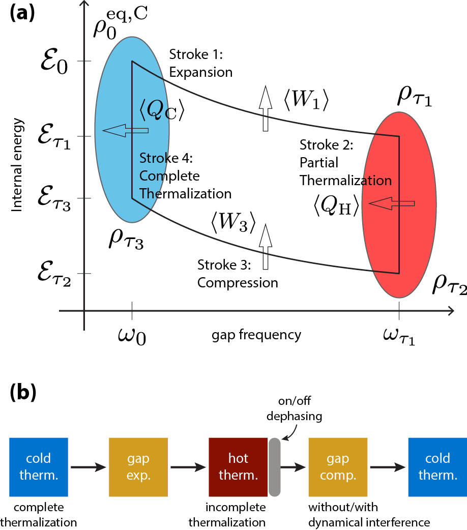
Figure 1: Engine cycle. (a) The working substance begins in the cold thermal state $\rho_{0}^{\text{eq,c}}$, with Hamiltonian $H_{0}$ and inverse temperature $\beta_{\text{c}}$. The working substance is driven by an adiabatic expansion which changes the Hamiltonian to $H_{\tau_{1}}$ and leads to the state $\rho_{\tau_{1}}$ at time $\tau_{1}$. The second stroke is comprised by hot thermalization, where the working substance interacts with a hot heat reservoir. The interaction time between the working substance and the heat reservoir is sufficiently small such that the thermalization is incomplete. The third stroke is an adiabatic compression changing the Hamiltonian from $H_{\tau_{1}}$ back to $H_{0}$. The fourth stroke is a complete thermalization with the cold heat reservoir. (b) Representation of the cycle with a dephasing operation in the energy basis after the incomplete thermalization. For this dephased engine, the states at the end of each stroke are $\rho_{0}^{\text{eq,c}}$, $\rho_{\tau_{1}}$, $\rho_{\tau_{2}}^{\text{deph}}$, and $\rho_{\tau_{3}}^{\text{deph}}$. This dephasing operation does not cost energy and erases the residual coherence of the engine.

In the first stroke, the energy gap of the working substance is increased by the driven Hamiltonian $H^{\text{exp}}\left(t\right)$ in a unitary dynamics. The working substance is assumed to be disconnected from the heat sources so that no energy is exchanged with them. In a realistic scenario, one could consider that the driven time is fast enough so that the energy exchanged between system and environment can be neglected and the driven dynamics is well described by a unitary evolution Peterson2018 ; Batalh=00003D0000E3o2014 ; Batalh=00003D0000E3o2015 ; Camati2016 . Hence, the state after the expansion stroke is given by $\rho_{\tau_{1}}=U_{\tau_{1},0}\rho_{0}^{\text{eq,c}}U_{\tau_{1},0}^{\dagger}$, where $U_{\tau_{1},0}=\mathcal{T}_{>}\exp\left\{-\frac{i}{\hbar}\int_{0}^{\tau_{1}}dt\,H^{\text{exp}}\left(t\right)\right\}$, $\mathcal{T}_{>}$ is the time-ordering operator, $t\in\left[0,\tau_{1}\right]$, and

$$H^{\text{exp}}\left(t\right)=\frac{\hbar\omega\left(t\right)}{2}\left[\cos\left(\frac{\pi t}{2\tau_{1}}\right)\sigma_{x}+\sin\left(\frac{\pi t}{2\tau_{1}}\right)\sigma_{z}\right],$$ (1)

with $\omega\left(t\right)=\omega_{0}\left(1-\frac{t}{\tau_{1}}\right)+\omega_{\tau_{1}}\left(\frac{t}{\tau_{1}}\right)$. We have chosen this protocol design because it has been recently employed in an experimental realization of the quantum Otto cycle with spin qubits Peterson2018 .

In the second stroke, the working substance interacts with a hot heat reservoir at inverse temperature $\beta_{\text{h}}=\left(k_{B}T_{\text{h}}\right)^{-1}$ and it undergoes a hot thermalization. The Hamiltonian is kept fixed at $H^{\text{hot}}\left(t\right)=H^{\text{exp}}\left(\tau_{1}\right)=H_{\tau_{1}}=\frac{\hbar\omega_{\tau_{1}}}{2}\sigma_{z}$ spanning the time interval $t\in\left[\tau_{1},\tau_{2}\right]$. Some stroke-driven models of quantum heat engines assume that this thermalization stroke is complete so that the system reaches thermal equilibrium state at the end of the stroke Wang2009 ; Altintas2015 . More precisely, in order to achieve this complete thermalization the condition $\tau_{2}-\tau_{1}=\tau_{\text{therm}}^{\text{h}}\gg\tau_{\text{relaxation}}^{\text{h}}$ should be satisfied, where $\tau_{\text{therm}}^{\text{h}}$ is the thermalization time and $\tau_{\text{relaxation}}^{\text{h}}$ is the relaxation time of the working substance with the hot heat reservoir.

Since our Hamiltonian does not commute with itself at different times, the first stroke generates coherence in the energy basis, all of which would be erased if such a complete thermalization was performed. Therefore, we consider a incomplete hot thermalization stroke, in which the thermalization time is of the order $\tau_{\text{therm}}^{\text{h}}\lesssim\tau_{\text{relaxation}}^{\text{h}}$. Performing an incomplete thermalization in our QOHE model will allow the working substance to retain a residual amount of coherence at the end of the hot thermalization (second stroke). Thus, there is some coherence generated at the first stroke that endures the thermalization stroke and, hence, will be present at the next driven (third) stroke. Therefore, the incomplete thermalization allows the dynamical transference of (some) coherence from the first to the third stroke. One of our goals is to study how the presence of this residual coherence in the dynamics of the cycle changes the thermodynamic quantities and the performance of the engine.

In the third stroke, the working substance energy gap is decreased to its original value during a unitarily driven dynamics. The compression Hamiltonian drives the qubit according to the condition $H^{\text{com}}\left(t\right)=H^{\text{exp}}\left(\tau_{1}+\tau_{2}-t\right)$ for the time interval $t\in\left[\tau_{2},\tau_{3}\right]$, with $\tau_{3}-\tau_{2}=\tau_{1}$ (“com” stands for compression). This condition guarantees that $H^{\text{com}}\left(t\right)$ takes the same values that $H^{\text{exp}}\left(t\right)$ did in the expansion stroke, but in inverse order (see Appendix A for a detailed explanation). Denoting by $\rho_{\tau_{2}}$ the final state of the second stroke, the state after the compression stroke is given by $\rho_{\tau_{3}}=V_{\tau_{3},\tau_{2}}\rho_{\tau_{2}}V_{\tau_{3},\tau_{1}}^{\dagger}$, where $V_{\tau_{3},\tau_{2}}=\mathcal{T}_{>}\exp\left\{-\frac{i}{\hbar}\int_{\tau_{2}}^{\tau_{3}}dt\,H^{\text{com}}\left(t\right)\right\}$ .

The fourth stroke is an undriven thermalization with a cold heat reservoir at inverse temperature $\beta_{\text{c}}$. The stroke spans the time interval $t\in\left[\tau_{3},\tau_{4}\right]$ and the Hamiltonian is kept fixed at $H^{\text{cold}}\left(t\right)=H^{\text{com}}\left(\tau_{3}\right)=H^{\text{exp}}\left(0\right)=H_{0}$. In order to close the engine cycle, i.e., $\rho_{\tau_{4}}=\rho_{0}^{\text{eq,c}}$, we consider complete thermalization in this stroke. Therefore, the cold thermalization time must satisfy the condition $\tau_{4}-\tau_{3}=\tau_{\text{therm}}^{\text{c}}\gg\tau_{\text{relaxation}}^{\text{c}}$.

The four relevant energetic quantities to analyze the thermodynamics of the engine are the following. The first- and third-stroke works $\left\langle W_{1}\right\rangle=\mathcal{E}_{\tau_{1}}-\mathcal{E}_{0}$ and $\left\langle W_{3}\right\rangle=\mathcal{E}_{\tau_{3}}-\mathcal{E}_{\tau_{2}}$, respectively, where $\mathcal{E}_{t}=\text{Tr}\left[H\left(t\right)\rho_{t}\right]$ denotes the mean instantaneous internal energy; and the hot and cold heats $\left\langle Q_{\text{h}}\right\rangle=\mathcal{E}_{\tau_{2}}-\mathcal{E}_{\tau_{1}}$ and $\left\langle Q_{\text{c}}\right\rangle=\mathcal{E}_{0}-\mathcal{E}_{\tau_{3}}$, which are the energies absorbed by the working substance during the interaction with the hot and cold heat reservoirs, respectively.

The dynamics of a qubit with a Hamiltonian $H\left(t\right)$ with energy gap $\hbar\omega$ interacting with a Markovian heat reservoir at inverse temperature $\beta$ can be described by the master equation Breuerbook2003 ; Chakraborty2016

$$\frac{d}{dt}\rho\left(t\right)= -\frac{i}{\hbar}\left[H\left(t\right),\rho\left(t\right)\right]$$

$$+\gamma_{\downarrow}\left[\Gamma_{\downarrow}\rho\left(t\right)\Gamma_{\uparrow}^{\dagger}-\frac{1}{2}\left\{\rho\left(t\right),\Gamma_{\uparrow}^{\dagger}\Gamma_{\downarrow}\right\}\right]$$

$$+\gamma_{\uparrow}\left[\Gamma_{\uparrow}\rho\left(t\right)\Gamma_{\downarrow}^{\dagger}-\frac{1}{2}\left\{\rho\left(t\right),\Gamma_{\downarrow}^{\dagger}\Gamma_{\uparrow}\right\}\right],$$ (2)

where $\gamma_{\downarrow}=\gamma_{0}\left(N_{\text{BE}}+1\right)$, $\gamma_{\uparrow}=\gamma_{0}N_{\text{BE}}$, $\gamma_{0}$ is the vacuum decay rate, $N_{\text{BE}}=\left(e^{\beta\hbar\omega}-1\right)^{-1}$ is the Bose-Einstein distribution, and $\Gamma_{\downarrow}$ ($\Gamma_{\uparrow}$) is the ladder operator in the energy eigenbasis that takes the excited (ground) state and transforms it into the ground (excited) state. The analytical solution of this equation is used to obtain the state $\rho_{\tau_{2}}$ after the incomplete hot thermalization stroke, and hence the thermodynamic relations with incomplete thermalization (for details see Appendix A).

The residual coherence that is transferred from the expansion to the compression strokes due to incomplete thermalization affects the thermodynamic quantities. In particular, as we discuss in Sec. III.2, a dynamical interference effect between the residual coherence and the coherence generated in the third stroke is revealed. In order to pinpoint the consequences of this interference effect, we benchmark our quantum engine with an alternative cycle without dynamical interference. In such a cycle a dephasing operation (in the energy basis) is employed to completely erase the residual coherence (after the second stroke), even for small thermalization times [see Fig. 1(b)]. This dephasing operation in the energy basis has no energetic cost, since it does not change the working substance mean internal energy.

In this way, we have two quantum engines, with and without (the dephased engine) dynamical interference, providing a fair benchmark for the investigation of the coherence effects along the cycle. Additionally, we employ the superscript “deph” to describe the quantities corresponding to the dephased engine cycle [see caption of Fig. 1(b)]. Further details concerning the dynamical interference effect are discussed in Sec. III.2.

III The role of quantum coherence in the irreversibility and performance of the engine

III.1 General description

The four relevant states $\rho_{0}^{\text{eq,c}}$, $\rho_{\tau_{1}}$, $\rho_{\tau_{2}}$, and $\rho_{\tau_{3}}$ (related to the four strokes) are the key states of the engine cycle that will be employed to completely analyze the performance of the proposed engine. For further reference, we call this set of states the key-working-substance states.

Before we proceed, it is convenient to establish a few important quantities that are going to be important throughout our analyzes. The (Kullback-Leibler-Umegaki) divergence between an arbitrary state $\rho$ and a reference state $\rho^{\text{ref}}$ is given by $D\left(\rho||\rho^{\text{ref}}\right)=-\text{Tr}\left[\rho\ln\rho^{\text{ref}}\right]-S\left(\rho\right)$, where $S\left(\rho\right)=-\text{Tr}\left[\rho\ln\rho\right]$ is the (von Neumann) entropy Umegaki1954 ; Vedral2002 ; Wilde2017 . We conventionally write the instantaneous Gibbs equilibrium state with Hamiltonian $H\left(t\right)$ and inverse temperature $\beta_{i}$ as $\rho_{t}^{\text{eq,}i}=e^{-\beta_{i}H\left(t\right)}/Z_{t}^{i}$, where $Z_{t}^{i}=\text{Tr }e^{-\beta_{i}H\left(t\right)}$ is the partition function and $i\in\left\{\text{c},\text{h}\right\}$ denotes the cold and hot thermal states, respectively. When the reference state of the divergence is some thermal state $\rho_{t}^{\text{eq,}i}$, we will call $D\left(\rho_{t}||\rho_{t}^{\text{eq,}i}\right)$ the thermal divergence.

For the driving strokes, we define the states $\rho_{t}^{\text{qs,}i}$, with $i\in\left\{\text{c},\text{h}\right\}$, as the states that would have been obtained if the driving was performed quasistatically (without transition among the instantaneous eigenstates) and if the initial state was the thermal state $\rho_{t_{0}}^{\text{eq,}i}$, where $t_{0}=0$ ($t_{0}=\tau_{2}$) for the expansion (compression) stroke. More explicitly, denoting by $\Ket{E_{n}^{t}}$ the instantaneous energy eigenstates, the two states associated with the end of the expansion and compression strokes are $\rho_{\tau_{1}}^{\text{qs,c}}=\sum_{n}p_{n}^{\text{eq,c},0}\Ket{E_{n}^{\tau_{1}}}\Bra{E_{n}^{\tau_{1}}}$ and $\rho_{\tau_{3}}^{\text{qs,h}}=\sum_{n}p_{n}^{\text{eq,h},\tau_{1}}\Ket{E_{n}^{0}}\Bra{E_{n}^{0}}$, where $p_{n}^{\text{eq,}i,t}$, with $i\in\left\{\text{c},\text{h}\right\}$, are the Boltzmann weights calculated with inverse temperature $\beta_{i}$ and Hamiltonian $H\left(t\right)$. When the reference state of the divergence is the quasistatically evolved state $\rho_{t}^{\text{qs,}i}$, we call $D\left(\rho_{t}||\rho_{t}^{\text{qs,}i}\right)$ the quasistatic divergence.

The efficiency of the quantum heat engine is given by the ratio of the net extracted work over the heat absorbed from the hot source, i.e., $\eta=-\left\langle W_{\text{net}}\right\rangle/\left\langle Q_{\text{h}}\right\rangle$, with $\left\langle W_{\text{net}}\right\rangle=\left\langle W_{1}\right\rangle+\left\langle W_{3}\right\rangle<0$ and $\left\langle Q_{\text{h}}\right\rangle>0$. The efficiency of the QOHE can be related to the total entropy produced ($\left\langle\Sigma_{\text{total}}\right\rangle$) in a cycle through Peterson2018 (see Appendix B)

$$\eta=\eta_{\text{Carnot}}-\frac{\left\langle\Sigma_{\text{total}}\right\rangle}{\beta_{\text{c}}\left\langle Q_{\text{h}}\right\rangle},$$ (3)

where $\eta_{\text{Carnot}}=1-\beta_{\text{h}}/\beta_{\text{c}}$.

The entropy produced during the incomplete thermalization with a Markovian heat reservoir (with constant Hamiltonian) is Deffner2011 $\left\langle\Sigma\right\rangle=D\left(\rho_{0}||\rho^{\text{eq}}\right)-D\left(\rho_{\tau}||\rho^{\text{eq}}\right)\geq 0$, where $\rho_{0}$ and $\rho_{\tau}$ are the initial and final states of the thermalization process and $\rho^{\text{eq}}$ is the Gibbs state. Applying these results to the engine cycle one finds (see Appendix B)

$$\left\langle\Sigma_{\text{total}}\right\rangle=D\left(\rho_{\tau_{1}}||\rho_{\tau_{1}}^{\text{eq,h}}\right)-D\left(\rho_{\tau_{2}}||\rho_{\tau_{2}}^{\text{eq,h}}\right)+D\left(\rho_{\tau_{3}}||\rho_{\tau_{3}}^{\text{eq,c}}\right),$$ (4)

which relates the total entropy of the cycle to the thermal divergences between the key-working-substance states. The quantity $\mathcal{L}_{\text{therm}}=\left\langle\Sigma_{\text{total}}\right\rangle/\beta_{\text{c}}\left\langle Q_{\text{h}}\right\rangle$ has been called the efficiency lag Peterson2018 (see also Ref. Campisi2016 ) since it quantifies the departure of the engine efficiency to the Carnot efficiency. In this paper, we will refer to $\mathcal{\mathcal{L}_{\text{therm}}}$ as the thermal efficiency lag in order to differentiate it from the other efficiency lag discussed below.

The total entropy production in Eq. (4) encompasses both the finite-time effects of the driven and thermalization dynamics of the engine cycle and directly accounts for the amount of irreversibility in the engine cycle. Through Eq. (3), since $\left\langle\Sigma_{\text{total}}\right\rangle$ is nonnegative, the quantum engine efficiency is upper bounded by the Carnot efficiency.

Let $\rho^{\text{ref}}=\sum_{n}\lambda_{n}\Pi_{n}$ denote the spectral decomposition of some reference state used to compute the divergence, where $\left\{\lambda_{n}\right\}$ are the eigenvalues and $\left\{\Pi_{n}\right\}$ are the eigenprojectors of $\rho^{\text{ref}}$. The divergence $D\left(\rho||\rho^{\text{ref}}\right)$ can be shown to be decomposed as Santos2017 ; Francica2017 ; Janzing2006 ; Lostaglio2015

$$D\left(\rho||\rho^{\text{ref}}\right)=D\left(\varepsilon\left(\rho\right)||\rho^{\text{ref}}\right)+\mathcal{C}\left(\rho\right),$$ (5)

where $\varepsilon\left(\cdot\right)=\sum_{n}\Pi_{n}\left(\cdot\right)\Pi_{n}$ is the full dephasing map and $\mathcal{C}\left(\rho\right)=S\left(\varepsilon\left(\rho\right)\right)-S\left(\rho\right)$ is the relative entropy of coherence (in the reference state basis) Aberg2006 ; Baumgratz2014 ; Streltsov2017 ; Winter2016 ; Singh2017 .

From now on, we conveniently assume that the energy basis of the instantaneous Hamiltonian $H\left(t\right)$ of the working substance is the relevant basis where the full dephasing $\varepsilon\left(\rho_{t}\right)$ and the relative entropy of coherence $\mathcal{C}\left(\rho_{t}\right)$ are computed. Applying the decomposition in Eq. (5) to Eq. (4), the entropy production can be written as

$$\left\langle\Sigma_{\text{total}}\right\rangle=\left\langle\Sigma_{\text{total}}^{\text{pop}}\right\rangle+\left\langle\Sigma_{\text{total}}^{\text{coh}}\right\rangle,$$ (6)

where

$$\left\langle\Sigma_{\text{total}}^{\text{pop}}\right\rangle= [D\left(\varepsilon\left(\rho_{\tau_{1}}\right)||\rho_{\tau_{1}}^{\text{eq,h}}\right)-D\left(\varepsilon\left(\rho_{\tau_{2}}\right)||\rho_{\tau_{2}}^{\text{eq,h}}\right)$$

$$+D\left(\varepsilon\left(\rho_{\tau_{3}}\right)||\rho_{\tau_{3}}^{\text{eq,c}}\right)]$$ (7)

and

$$\left\langle\Sigma_{\text{total}}^{\text{coh}}\right\rangle=\mathcal{C}\left(\rho_{\tau_{1}}\right)-\mathcal{C}\left(\rho_{\tau_{2}}\right)+\mathcal{C}\left(\rho_{\tau_{3}}\right)$$ (8)

quantify the contribution of the populations ($\left\langle\Sigma_{\text{total}}^{\text{pop}}\right\rangle$) and coherences ($\left\langle\Sigma_{\text{total}}^{\text{coh}}\right\rangle$) of the key-working-substance states to the total entropy production, respectively. These terms show explicitly how the coherence of the key-working-substance states of the QOHE contributes to the engine irreversibility and, thus, to the engine efficiency by means of Eq. (3). Equation (3) is obtained assuming a closed cycle, without assuming any particular model for the quantum working substance. Before we discuss the effects of coherence and the dynamical interference in the engine performance, we present a particular relation for a QOHE fueled by a single-qubit working substance.

When all strokes take infinite time, i.e., the engine operates in the quasistatic regime, it does not produce any quantum friction and, thus, achieves its maximum efficiency, producing minimum entropy along the cycle. For a QOHE, the maximum efficiency is given by the quantum Otto efficiency $\eta_{\text{Otto}}=1-\omega_{0}/\omega_{\tau_{1}}$ Kosloff2017 .

For a single-qubit working substance, we obtained the expression (see Appendix C and Appendix D)

$$\eta=\eta_{\text{Otto}}-\frac{\mathcal{F}}{\beta_{\text{c}}\left\langle Q_{\text{h}}\right\rangle},$$ (9)

where

$$\mathcal{F}= D\left(\rho_{\tau_{1}}||\rho_{\tau_{1}}^{\text{qs,c}}\right)$$

$$+\frac{\omega_{0}\beta_{\text{c}}}{\omega_{\tau_{1}}\beta_{\text{h}}}\left[D\left(\rho_{\tau_{3}}||\rho_{\tau_{3}}^{\text{qs,h}}\right)-D\left(\rho_{\tau_{2}}||\rho_{\tau_{2}}^{\text{eq,h}}\right)\right]$$ (10)

quantifies the quantum friction ($\mathcal{F}\geq 0$) in the quantum Otto heat engine Marcela . It contains two quasistatic divergences (associated with both driven strokes) and the thermal divergence of the state incompletely thermalized. In the limit that $\tau_{1}$, $\tau_{2}$, and $\tau_{3}$ are infinitely large, all divergences are identically zero. This means that no quantum friction implies $\mathcal{F}=0$, which implies $\eta=\eta_{\text{Otto}}$. We will refer to the quantity $\mathcal{L}_{\text{qs}}=\mathcal{F}/\beta_{\text{c}}\left\langle Q_{\text{h}}\right\rangle$ as the quasistatic efficiency lag.

Employing the same reasoning that leads to Eq. (5), we can split the quantum friction into two contributions

$$\mathcal{F}=\mathcal{F}^{\text{pop}}+\mathcal{F}^{\text{coh}},$$ (11)

where

$$\mathcal{F}^{\text{pop}}= D\left[\varepsilon\left(\rho_{\tau_{1}}\right)||\rho_{\tau_{1}}^{\text{qs,c}}\right]$$

$$+\frac{\omega_{0}\beta_{\text{c}}}{\omega_{\tau_{1}}\beta_{\text{h}}}\left\{D\left[\varepsilon\left(\rho_{\tau_{3}}\right)||\rho_{\tau_{3}}^{\text{qs,h}}\right]-D\left[\varepsilon\left(\rho_{\tau_{2}}\right)||\rho_{\tau_{2}}^{\text{eq,h}}\right]\right\}$$ (12)

and

$$\mathcal{F}^{\text{coh}}=\mathcal{C}\left(\rho_{\tau_{1}}\right)+\frac{\omega_{0}\beta_{\text{c}}}{\omega_{\tau_{1}}\beta_{\text{h}}}\left[\mathcal{C}\left(\rho_{\tau_{3}}\right)-\mathcal{C}\left(\rho_{\tau_{2}}\right)\right]$$ (13)

quantify the contribution of the populations ($\mathcal{F}^{\text{pop}}$) and coherences ($\mathcal{F}^{\text{coh}}$) of the key-working-substance states, respectively.

The entropy production and quantum friction in Eqs. (4) and (10) have been decomposed into a population and a coherent contribution with respect to the relevant instantaneous energy basis. However, this does not mean that the population part does not depend on the coherences whatsoever. For a driving that generates coherence in the instantaneous energy eigenbasis, such as our first and third driven strokes, the populations of the final state depend on the way that coherence was generated, i.e., depend on the process. Therefore, the separation into the population and coherent contributions is with respect to the populations and coherences of the key-working-substance states.

Combining Eqs. (3) and (9) one can find the relation Peterson2018 ; Marcela

$$\left\langle\Sigma_{\text{total}}\right\rangle=\beta_{\text{c}}\left\langle Q_{\text{h}}\right\rangle\left[\eta_{\text{Carnot}}-\eta_{\text{Otto}}\right]+\mathcal{F}$$ (14)

between the total entropy production and the quantum friction in a QOHE. The minimum entropy production is obtained when there is no quantum friction, i.e., when the engine runs in the quasistatic regime, and it is given by $\left\langle\Sigma_{\text{total}}^{\text{min}}\right\rangle=\beta_{\text{c}}\left\langle Q_{\text{h}}^{\text{qs}}\right\rangle\left[\eta_{\text{Carnot}}-\eta_{\text{Otto}}\right]$, where $\left\langle Q_{\text{h}}^{\text{qs}}\right\rangle$ is the heat absorbed in the quasistatic limit of the cycle.

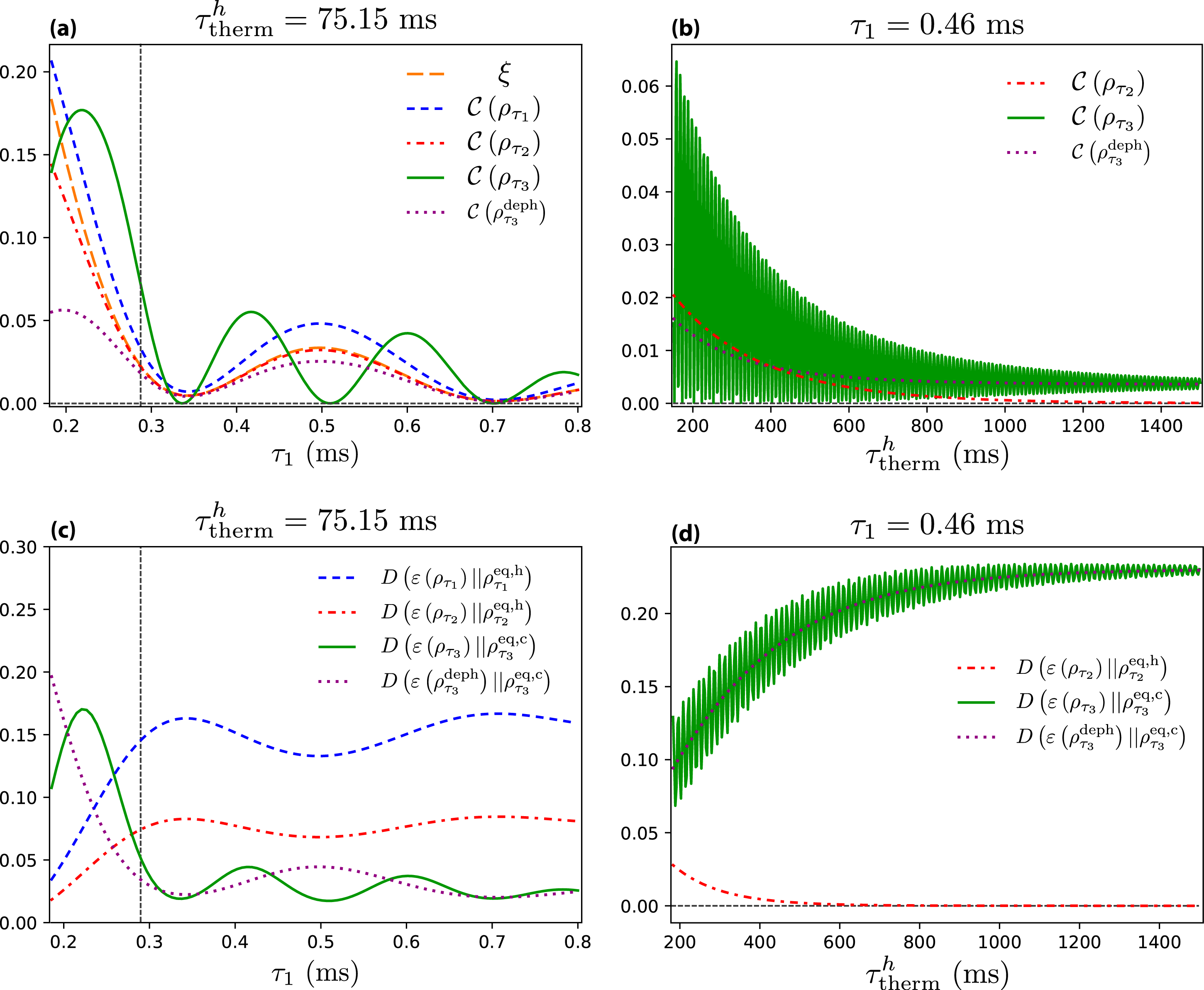
Figure 2: Dynamics of the coherences. (a) The relative entropy of coherences of the key-working-substance states $\mathcal{C}\left(\rho_{\tau_{1}}\right)$ (blue dashed line), $\mathcal{C}\left(\rho_{\tau_{2}}\right)$ (red dash-dotted line), and $\mathcal{C}\left(\rho_{\tau_{3}}\right)$ (green solid line) for the original and $\mathcal{C}\left(\rho_{\tau_{3}}^{\text{deph}}\right)$ (purple dotted line) for dephased engine cycles. Additionally, the energy transition probability $\xi^{\text{exp}}\left(\tau_{1},0\right)$ (orange long-dashed line) is also shown. All quantities are plotted assuming a fixed thermalization time $\tau_{\text{therm}}^{\text{h}}=75.15\text{ ms}$ and varying the driving time $\tau_{1}$. The engine works as a heat engine for the parameters on the right of the dashed vertical line. (b) The relative entropy of coherence of the relevant key-working-substance states as a function of the thermalization time $\tau_{\text{therm}}^{\text{h}}$ for fixed driving time $\tau_{1}=0.46\text{ ms}$. (c) The population component of the thermal divergence of the key-working-substance states, $D\left(\varepsilon\left(\rho_{\tau_{1}}\right)||\rho_{\tau_{1}}^{\text{eq,h}}\right)$ (blue dashed line), $D\left(\varepsilon\left(\rho_{\tau_{2}}\right)||\rho_{\tau_{2}}^{\text{eq,h}}\right)$ (red dash-dotted line), and $D\left(\varepsilon\left(\rho_{\tau_{3}}\right)||\rho_{\tau_{3}}^{\text{eq,c}}\right)$ (green solid line) for the original and $D\left(\varepsilon\left(\rho_{\tau_{3}}^{\text{deph}}\right)||\rho_{\tau_{3}}^{\text{eq,c}}\right)$ (purple dotted line) for the dephased engine cycles. All quantities are plotted assuming a fixed thermalization time $\tau_{\text{therm}}^{\text{h}}=75.15\text{ ms}$ and varying the driving time $\tau_{1}$. (d) The population component of the thermal divergence of the key-working-substance states as a function of the thermalization time $\tau_{\text{therm}}^{\text{h}}$ for fixed driving time $\tau_{1}=0.46\text{ ms}$. The map $\varepsilon$ is the full dephasing operation as explained in Eq. (5). All entropic quantities are computed in the natural unit of information (nat).

The engine average power output per cycle is given by $P_{\text{tot}}=-\left\langle W_{\text{net}}\right\rangle/\tau_{\text{cycle}}$, where $\tau_{\text{cycle}}=\tau_{4}=\tau_{1}+\tau_{\text{therm}}^{\text{h}}+\tau_{1}+\tau_{\text{therm}}^{\text{c}}$ is the cycle time duration. The relation between the efficiency and power is given by $P_{\text{tot}}=\eta\left\langle Q_{\text{h}}\right\rangle/\tau_{\text{cycle}}$ . With this expression and Eqs. (3) and (9), the extractable power can be written in terms of the entropy production or quantum friction as

$$P_{\text{tot}}=\frac{\eta_{\text{Carnot}}\left\langle Q_{\text{h}}\right\rangle}{\tau_{\text{cycle}}}-\frac{\left\langle\Sigma_{\text{total}}\right\rangle}{\beta_{\text{c}}\tau_{\text{cycle}}}$$ (15)

and

$$P_{\text{tot}}=\frac{\eta_{\text{Otto}}\left\langle Q_{\text{h}}\right\rangle}{\tau_{\text{cycle}}}-\frac{\mathcal{F}}{\beta_{\text{c}}\tau_{\text{cycle}}},$$ (16)

respectively. Then, using the decompositions in Eqs. (6) and (11), the power can be written in terms of the relative entropy of coherence of the key-working-substance states.

The expressions discussed above for the finite-time dynamics of the engine explicitly show how the energy coherence of the key-working-substance states contributes to the engine performance and irreversibility. At this point it is important to clarify that, for an engine which generates coherence in the energy basis during the first stroke, a complete thermalization with the hot heat reservoir would imply $D\left(\rho_{\tau_{2}}||\rho_{\tau_{2}}^{\text{eq,h}}\right)=0$ and $\mathcal{C}\left(\rho_{\tau_{2}}\right)=0$ identically. Hence, the presence of coherence would always contribute to an increase in irreversibility (both entropy production and quantum friction) and a decrease in the engine performance, when compared with an engine where the driven strokes do not produce coherence.

On the other hand, if the thermalization is incomplete, the contribution of the incompletely thermalized state $\rho_{\tau_{2}}$ (after the second stroke) is manifested through the term $D\left(\rho_{\tau_{2}}||\rho_{\tau_{2}}^{\text{eq,h}}\right)$. Such a thermal divergence contributes to decrease both the entropy production and quantum friction as can verified in Eqs. (4) and (10). This means that the residual coherence after the incomplete thermalization (second stroke), quantified by $\mathcal{C}\left(\rho_{\tau_{2}}\right)$ in Eqs. (10) and (13), helps decrease the irreversibility and, consequently, increase the engine performance in comparison to an engine that generates coherence and has complete thermalization. In the next section, we will show that not only does the residual coherence directly decrease the entropy production and quantum friction but it also gives rise to a dynamical interference effect that also helps decrease the irreversibility of the engine.

III.2 Numerical analysis

Let us now investigate the effects of the coherence in the key-working-substance states during the cycle, and in particular the residual coherence, employing numerical simulations. In this analysis, we consider energy scales compatible with quantum thermodynamics experiments in nuclear magnetic resonance setups Peterson2018 ; Batalh=00003D0000E3o2014 ; Batalh=00003D0000E3o2015 ; Camati2016 ; Micadei2017 . The initial and final frequency gaps of the expansion stroke will be chosen as $\omega_{0}/2\pi=2.0\text{ kHz}$ and $\omega_{\tau_{1}}/2\pi=3.6\text{ kHz}$, respectively. The chosen temperatures are such that the thermal energy scale of the cold (hot) heat reservoir is half (double) the energy gap of the working substance at the time of the interaction with the heat source. More precisely, the cold and hot inverse temperatures will be chosen as $\beta_{\text{c}}=2/\left(\hbar\omega_{0}\right)$ and $\beta_{\text{h}}=1/\left(2\hbar\omega_{\tau_{1}}\right)$, respectively.

We assume that a complete thermalization with the cold environment is approximately achieved at a finite time satisfying the condition $\tau_{\text{therm}}^{\text{c}}\gg\tau_{\text{relaxation}}^{\text{c}}$. We also consider that the interaction time with the hot reservoir is smaller than or of the same order as the relaxation time of the hot environment $\tau_{\text{therm}}^{\text{h}}\apprle\tau_{\text{relaxation}}^{\text{h}}$, which results in an incomplete thermalization with the hot environment in the engine cycle. The strength of the interaction of the working substance with the hot and cold heat reservoirs, namely, the vacuum decay rate, will be assumed as $\gamma_{0}^{\text{h}}=\gamma_{0}^{\text{c}}=1\text{Hz}$, which implies the relaxation time $\tau_{\text{relaxation}}^{\text{h}}=244.92\text{ ms}$ and $\tau_{\text{relaxation}}^{\text{c}}=761.59\text{ ms}$. In order to reach approximately a complete thermalization at the end of the fourth stroke, we considered the cold thermalization time as $\tau_{\text{therm}}^{\text{c}}\approx 6.56\times\tau_{\text{relaxation}}^{\text{c}}$. In this case, the working substance approximately returns to the cold Gibbs state. The trace distance between the final state of the fourth stroke and the cold Gibbs state is approximately $\frac{1}{2}\text{Tr}\left|\rho_{\tau_{4}}-\rho_{0}^{\text{eq,c}}\right|\simeq 10^{-2}$.

Figures. 2(a) and 2(b) display the relative entropies of coherence as a function of the driving time $\tau_{1}$ and the thermalization time $\tau_{\text{therm}}^{\text{h}}$, respectively. In Fig. 2(a) one can see that the relative entropy of coherence at the end of the first and second strokes are qualitatively similar. The residual coherence $\mathcal{C}\left(\rho_{\tau_{2}}\right)$ is smaller than $\mathcal{C}\left(\rho_{\tau_{1}}\right)$ due to a partial decrease of $\mathcal{C}\left(\rho_{\tau_{1}}\right)$ set by the incomplete thermalization.

Recall that the quantities for the dephased engine cycle are labeled by the superscript “deph” [see caption of Fig. 1(b)]. The coherence at the end of the third stroke of the dephased engine cycle $\mathcal{C}\left(\rho_{\tau_{3}}^{\text{deph}}\right)$ behaves qualitatively as $\mathcal{C}\left(\rho_{\tau_{1}}\right)$ and $\mathcal{C}\left(\rho_{\tau_{2}}\right)$, even being smaller than $\mathcal{C}\left(\rho_{\tau_{2}}\right)$. Note how the behavior of the coherence at the end of the third stroke in the original (not dephased) engine cycle $\mathcal{C}\left(\rho_{\tau_{3}}\right)$ is different. This qualitative difference comes from the interference between the residual coherence and the coherence generated at the third stroke [see green and purple dotted curves in Figs. 2(a) and 2(b)].

Figures 2(c) and 2(d) show the population component of the thermal divergence as a function of the driving time $\tau_{1}$ and the thermalization time $\tau_{\text{therm}}^{\text{h}}$, respectively. Again, in 2(c) one can note that the curves for the population component of the thermal divergence at the end of the first and second strokes are similar. Furthermore, the behaviors of the population components of the thermal divergences at the end of the third stroke of the original [$D\left(\varepsilon\left(\rho_{\tau_{3}}\right)||\rho_{\tau_{3}}^{\text{eq,c}}\right)$] and the dephased [$D\left(\varepsilon\left(\rho_{\tau_{3}}^{\mbox{deph}}\right)||\rho_{\tau_{3}}^{\text{eq,c}}\right)$] engines are qualitatively different. Such a difference also comes from the dynamical interference effect, highlighting that the populations of the key-working-substance states are not independent from the generated coherence during the strokes [see green and dotted-purple curves in Figs. 2(c) and 2(d)].

The amount of coherence as measured by $\mathcal{C}\left(\rho_{\tau_{2}}\right)$ decays exponentially with the thermalization time $\tau_{\text{therm}}^{\text{h}}$ [see Fig. 2(b)]. On the other hand, the coherence $\mathcal{C}\left(\rho_{\tau_{3}}\right)$ oscillates quickly due to the interference of the residual coherence $\mathcal{C}\left(\rho_{\tau_{2}}\right)$ and the coherence generated by the driven dynamics in the compression stroke. As the thermalization time increases, the oscillating amplitudes of $\mathcal{C}\left(\rho_{\tau_{3}}\right)$ become less pronounced, going asymptotically to zero, in which case the coherence $\mathcal{C}\left(\rho_{\tau_{3}}\right)$ approaches $\mathcal{C}\left(\rho_{\tau_{3}}^{\text{deph}}\right)$ because the coherence $\mathcal{C}\left(\rho_{\tau_{1}}\right)$ is increasingly erased. In the expressions for the efficiency and power output, the term $\mathcal{C}\left(\rho_{\tau_{2}}\right)-\mathcal{C}\left(\rho_{\tau_{3}}\right)$ explicitly appears, suggesting that whenever $\mathcal{C}\left(\rho_{\tau_{2}}\right)\geq\mathcal{C}\left(\rho_{\tau_{3}}\right)$ efficiency and power output can be enhanced, compared to the dephased engine performance. From Fig. 2(b) we can see that the rapid oscillations make this inequality be satisfied for very narrow time intervals. Such a behavior will be present in the efficiency and power output as will be seen shortly.

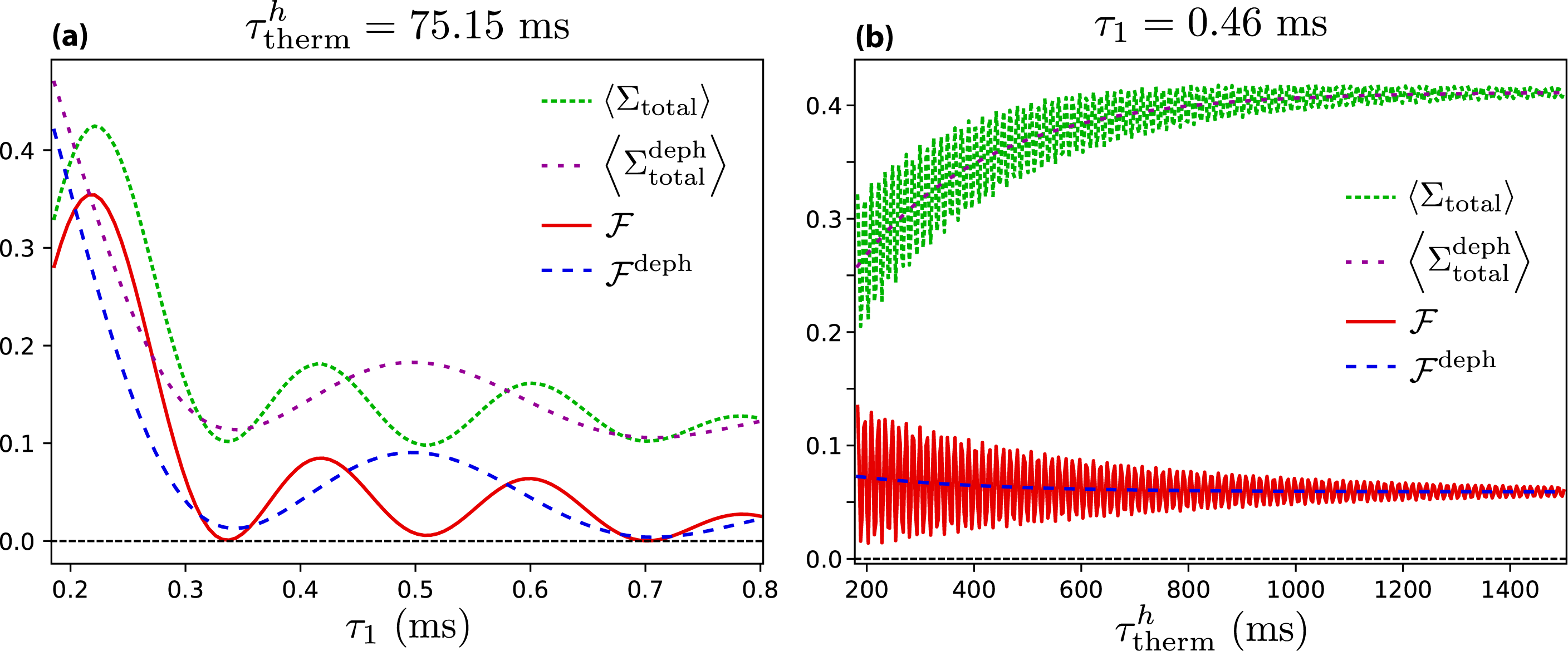
Figure 3: Entropy production and quantum friction as a function of the driving time $\tau_{1}$ (a) and thermalization time $\tau_{\text{therm}}^{\text{h}}$ (b). Total entropy production of the engine with and without dynamical interference is $\left\langle\Sigma_{\text{total}}\right\rangle$ and $\left\langle\Sigma_{\text{total}}^{\text{deph}}\right\rangle$, respectively. Similarly, the quantum friction of the engine with and without dynamical interference is $\mathcal{F}$ and $\mathcal{F}^{\text{deph}}$, respectively. All entropic quantities are computed in the natural unit of information (nat).

In Fig. 2(d), one can observe that $D\left(\varepsilon\left(\rho_{\tau_{2}}\right)||\rho_{\tau_{2}}^{\text{eq,h}}\right)$ approaches zero as the thermalization time increases, as expected. On the other hand, the oscillatory profile in $D\left(\varepsilon\left(\rho_{\tau_{3}}\right)||\rho_{\tau_{3}}^{\text{eq,c}}\right)$ (green solid line) in comparison to $D\left(\varepsilon\left(\rho_{\tau_{3}}^{\text{deph}}\right)||\rho_{\tau_{3}}^{\text{eq,c}}\right)$ (purple dotted line) is solely due to the interference of the residual coherence and the coherence generated during the third stroke. It is interesting to note that, in the present scenario, the relative entropies of coherence and the population components of the thermal divergences can not be varied in an independent way varying the stroke parameters. For instance, in Fig. 2(a) and 2(c), $\mathcal{C}\left(\rho_{\tau_{3}}\right)$ and $D\left(\varepsilon\left(\rho_{\tau_{3}}^{\text{deph}}\right)||\rho_{\tau_{3}}^{\text{eq,c}}\right)$ oscillate roughly in phase while $\mathcal{C}\left(\rho_{\tau_{2}}\right)$ and $D\left(\varepsilon\left(\rho_{\tau_{2}}\right)||\rho_{\tau_{2}}^{\text{eq,h}}\right)$ oscillate roughly out of phase. This aspect highlights the interrelation between the coherences and populations.

Figures 3(a) and 3(b) display the total entropy production and quantum friction of the original (with dynamical interference) and the dephased (without dynamical interference) engines as a function of the driving time $\tau_{1}$ and the thermalization time $\tau_{\text{therm}}^{\text{h}}$, respectively. The entropy production $\left\langle\Sigma_{\text{total}}\right\rangle$ and quantum friction $\mathcal{F}$ differ by a term containing the heat absorbed by the working substance from the hot heat reservoir and the difference between the Carnot and Otto efficiencies [see Eq. (14)]. The difference of the efficiency lags, on the other hand, is constant with respect to $\tau_{1}$ or $\tau_{\text{therm}}^{\text{h}}$, $\mathcal{L}_{\text{therm}}-\mathcal{L}_{\text{qs}}=\eta_{\text{Carnot}}-\eta_{\text{Otto}}$.

Comparing the entropy production and quantum friction of either the original or the dephased engine to each other, Fig. 3(a) shows that their qualitative behaviors are the same with respect to the driving time $\tau_{1}$. Moreover, note that the quantities for the original and dephased engine change in different timescales. The original engine quantities contain the effect of the dynamical interference and behave similarly to the relative entropy of coherence $C\left(\rho_{\tau_{3}}\right)$ and population divergence $D\left[\varepsilon\left(\rho_{\tau_{3}}\right)||\rho_{\tau_{3}}^{\text{eq,c}}\right]$ [see Figs. 2(a) and 2(c)].

The oscillation timescale of entropy production and quantum friction with respect to the thermalization time $\tau_{\text{therm}}^{\text{h}}$ shown in Fig. 3(b) also agree with the relative entropy of coherence and population divergence [compare with Figs. 2(b) and 2(d)]. However, entropy production increases while the quantum friction decreases the more the working substance reaches the thermal state. The closer a system reaches to the thermal state the larger the entropy produced Deffner2011 , so the increase in Fig. 3(b) is expected. Increasing the thermalization time decreases the coherence generated in the third stroke [see Fig. 2(b)]. The decrease in quantum friction is associated with the decrease in the total amount of coherence generated in the engine, showing the deep connection of quantum friction and energy coherence.

Our results generalize and qualitatively explain some previous findings in the literature. For instance, in Refs. Rezek2010 ; Feldmann2006 noise has been used to improve the quantum engine efficiency. Here we observe that, if the noise is such that it decreases the contribution of either $\mathcal{C}\left(\rho_{\tau_{1}}\right)$ or $\mathcal{C}\left(\rho_{\tau_{3}}\right)$, the efficiency can be enhanced. Moreover, quite a few papers have considered the so-called energy entropy of the working substance as a measure of quantum friction Feldmann2004 ; Rezek2010 ; Feldmann2012 ; Zagoskin2012 . Although not directly connected in these works, the difference between what these authors called energy entropy and the von Neumann entropy is nothing but the relative entropy of coherence. The present paper elucidates how this energy entropy was related to quantum friction in Refs. Feldmann2004 ; Rezek2010 ; Feldmann2012 ; Zagoskin2012 , namely, through the relative entropy of coherence in Eqs. (10), (11), and (13). In Refs. Feldmann2006 ; Rezek2006 ; Feldmann2012 ; Thomas2014 ; Correa2015 , quantum friction has been somewhat related to the presence of coherence. Reference Feldmann2012 , for instance, employed the $l_{1}$ norm of coherence to quantify quantum friction. Our results complement these findings by providing a concrete relation that elucidates how energy coherence is linked to quantum friction by means of the quasistatic and thermal divergences.

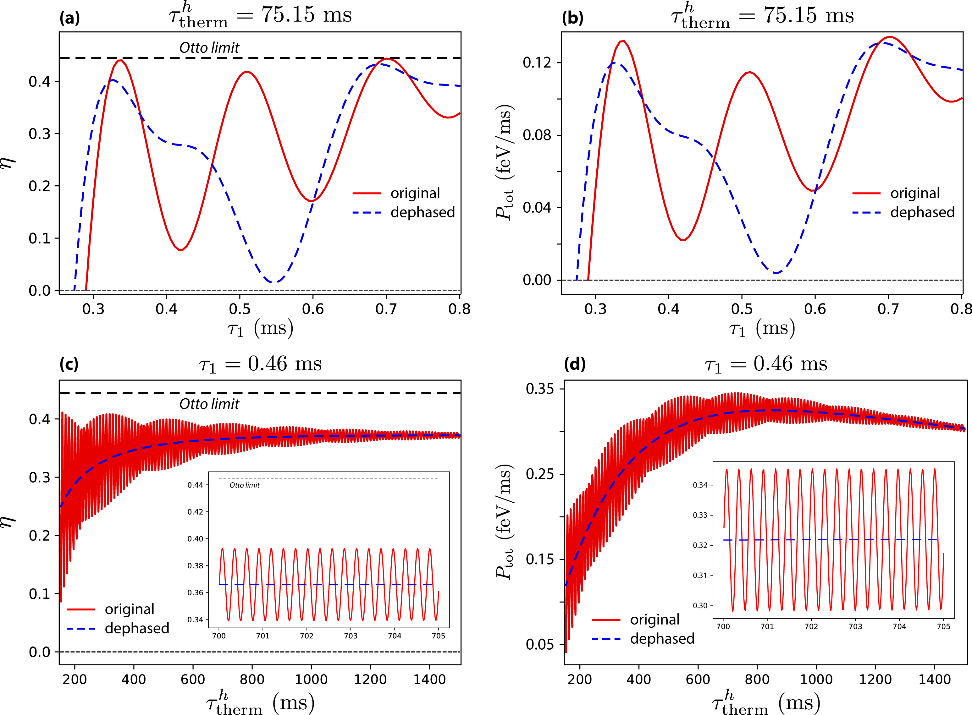
Figure 4: Efficiency and power output. (a) and (b) The engine efficiency and power output as a function of the driving time $\tau_{1}$ for the fixed thermalization time $\tau_{\text{therm}}^{\text{h}}=75.15\text{ ms}$, respectively. (c) and (d) The engine efficiency and power output as a function of the thermalization time $\tau_{\text{therm}}^{\text{h}}$ for the fixed driving time $\tau_{1}=0.46\text{ ms}$, respectively. In all figures, the efficiency and power output of the original and dephased engine cycle are depicted in red solid line and blue dashed line, respectively.

We have seen some effects of the interference of coherence in the previous plots and discussions. We further analyze this phenomenon by showing exactly how it contributes energetically to the thermodynamic quantities in the quantum cycle. The following relations have all been obtained assuming a single qubit as working substance, as described in Sec. II.

Let us denote by $E_{n}^{t}$ and $\Ket{E_{n}^{t}}$ the instantaneous eigenenergies and eigenstates of the engine Hamiltonian, respectively, where the index $n=0$ ($n=1$) stands for the ground (excited) state. The energy transition probability in the first stroke is given by

$$p_{\tau_{1},0}^{\text{exp}}\left(1|0\right)=\left|\Bra{E_{1}^{\tau_{1}}}U_{\tau_{1},0}\Ket{E_{0}^{0}}\right|^{2}=\xi\left(\tau_{1},0\right).$$ (17)

Evaluating the first-stroke work and the second-stroke heat one obtains $\left\langle W_{1}\right\rangle=\frac{1}{2}\left\{\hbar\omega_{0}-\hbar\omega_{\tau_{1}}\left[1-2\xi\left(\tau_{1},0\right)\right]\right\}g_{\text{c}}$ and $\left\langle Q_{\text{h}}\right\rangle=\frac{1}{2}\hbar\omega_{\tau_{1}}\left\{\left[1-2\xi\left(\tau_{1},0\right)\right]g_{\text{c}}+r_{z}\left(\tau_{2}\right)\right\}$, respectively, where $g_{\text{c}}=\tanh\left(\frac{1}{2}\beta_{\text{c}}\hbar\omega_{0}\right)$ and $r_{z}\left(\tau_{2}\right)=\text{Tr}\left[\sigma_{z}\rho_{\tau_{2}}\right]$ is the $z$ component of the qubit Bloch vector associated with $\rho_{\tau_{2}}$. In particular, for a complete thermalization, this Bloch vector component will be $r_{z}\left(\tau_{2}\rightarrow\infty\right)=g_{\text{h}}=\tanh\left(\frac{1}{2}\beta_{\text{h}}\hbar\omega_{\tau_{1}}\right)$.

The third-stroke work can be evaluated as

$$\left\langle W_{3}\right\rangle=\frac{1}{2}\left\{\hbar\omega_{0}\left[1-2\zeta\left(\tau_{3},\tau_{2}\right)\right]-\hbar\omega_{\tau_{1}}\right\}r_{z}\left(\tau_{2}\right)+\mathcal{E}_{\text{inter}},$$ (18)

where $\zeta\left(\tau_{3},\tau_{2}\right)=p_{\tau_{3},\tau_{2}}^{\text{com}}\left(1|0\right)=\left|a_{10}^{\text{com}}\left(\tau_{3},\tau_{2}\right)\right|^{2}$ is the third-stroke energy transition probability, $a_{mn}^{\text{com}}\left(\tau_{3},\tau_{2}\right)=\Bra{E_{m}^{\tau_{3}}}V_{\tau_{3},\tau_{2}}\Ket{E_{n}^{\tau_{2}}}$ is the energy probability amplitude, and

$$\mathcal{E}_{\text{inter}}= 2\sum_{n}E_{n}^{0}e^{-\gamma^{\text{h}}\tau_{\text{therm}}^{\text{h}}/2}$$

$$\times\text{Re}\left\{\rho_{10}\left(\tau_{1}\right)e^{i\tau_{\text{therm}}^{\text{h}}\omega_{\tau_{1}}}a_{n1}^{\text{com}}a_{n0}^{\text{com}*}\right\}$$ (19)

is the energy contribution due to the interference between the residual coherence and the coherence generated in the third stroke (see Appendix E). In Eq. (19), $\gamma^{\text{h}}=\gamma_{0}^{\text{h}}\left(2N_{\text{BE}}^{\text{h}}+1\right)$ is the total decay rate of the qubit after the interaction with the hot heat reservoir, and $\rho_{10}\left(\tau_{1}\right)=\Bra{E_{1}^{\tau_{1}}}\rho_{\tau_{1}}\Ket{E_{0}^{\tau_{1}}}$ is one of the coherence elements of the qubit state in the instantaneous energy basis at the beginning of the second stroke.

The contribution $\mathcal{E}_{\text{inter}}$ in Eq. (18) comes exclusively from the residual coherence at the end of the second stroke, i.e., the coherence that was not completely erased by incomplete thermalization. If the thermalization was complete ($\tau_{\text{therm}}^{\text{h}}\rightarrow\infty$) then $\mathcal{E}_{\text{inter}}=0$. Since the third-stroke work is present in the engine efficiency and power output, it is clear that $\mathcal{E}_{\text{inter}}$ [Eq. (19)] changes the engine performance. Next, we focus on how exactly $\mathcal{E}_{\text{trans}}$ changes the relevant quantities.

The internal energies of the original and dephased QOHEs are related as: $\mathcal{E}_{0}=\mathcal{E}_{0}^{\text{deph}}$, $\mathcal{E}_{\tau_{1}}=\mathcal{E}_{\tau_{1}}^{\text{deph}}$, $\mathcal{E}_{\tau_{2}}=\mathcal{E}_{\tau_{2}}^{\text{deph}}$, and $\mathcal{E}_{\tau_{3}}=\mathcal{E}_{\tau_{3}}^{\text{deph}}+\mathcal{E}_{\text{inter}}$, where $\mathcal{E}_{\text{trans}}$ is given in Eq. (19). From these relations we can readily obtain the efficiency

$$\eta=\eta^{\text{deph}}-\frac{\mathcal{E}_{\text{inter}}}{\left\langle Q_{\text{h}}\right\rangle}$$ (20)

and power

$$P_{\text{tot}}=P_{\text{tot}}^{\text{deph}}-\frac{\mathcal{E}_{\text{inter}}}{\tau_{\text{cycle}}}$$ (21)

of the original engine written with respect to the efficiency and power of the dephased engine. Furthermore, from Eq. (20) and Eqs. (3) and (9), we can also obtain how the entropy production and quantum friction change due to the residual coherence; they are given by

$$\left\langle\Sigma_{\text{total}}\right\rangle=\left\langle\Sigma_{\text{total}}^{\text{deph}}\right\rangle+\beta_{\text{c}}\mathcal{E}_{\text{inter}}$$ (22)

and

$$\mathcal{F}=\mathcal{F}^{\text{deph}}+\beta_{\text{c}}\mathcal{E}_{\text{inter}},$$ (23)

respectively. All these last four equations show how the performance of the engine is affected by the interference between the residual coherence and the coherence generated in the third stroke, quantified by $\mathcal{E}_{\text{inter}}$. Next, we see this effect in our particular QOHE.

In Fig. 4(a) we compare the efficiency of the original QOHE (red solid line), which contains the dynamical interference effect, and the dephased QOHE (blue dashed line), which does not contain the interference effect, as a function of the driving time $\tau_{1}$ for a fixed incomplete thermalization time $\tau_{\text{therm}}^{\text{h}}=75.15\text{ ms}$ ($\tau_{\text{therm}}^{\text{h}}\approx 0.31\times\tau_{\text{relaxation}}^{\text{h}}$). Observing Fig 4(a), we can note that the original QOHE may perform better or worse than the dephased QOHE. In this parameter regime, the dynamical interference can make the original QOHE perform about $20$ times more efficiently than the dephased QOHE in the intermediate region of the plot. Furthermore, even for such a small thermalization time (about 1/3 of the relaxation time), the efficiency of the original QOHE reaches values very close to Otto’s efficiency. This is a consequence of the small quantum friction generated by the engine cycle as seen in Fig. 3(a).

A similar behavior can be observed in the power output [see Fig. 4(b)]. The power output of the original QOHE can also be greater or smaller than the power of the dephased QOHE. Note that the efficiency and power of both the original and dephased QOHE oscillate. Since, by construction, there is no interference effect in the dephased QOHE, these oscillations are not a manifestation of the residual coherence alone. They arise from the choice of the driving Hamiltonian.

Now let us consider a fixed driving time $\tau_{1}$. In this case, the efficiency and power of the original QOHE oscillate as function of the thermalization time $\tau_{\text{therm}}^{\text{h}}$ as displayed in Figs. 4(c) and (d). Comparing them to Figs. 2(a) and (b), the oscillations in Figs. 4(c) and (d) occur strictly due to interference between the residual coherence and the coherence generated in the third stroke. The effect of this interference is damped as the thermalization time $\tau_{\text{therm}}^{\text{h}}$ increases [see Eq. (19)].

For an engine that generates coherence in the first stroke, the interference effect may or may not contribute to increase the engine performance and function as a quantum lubricant. A fine control over the driving and thermalization times is paramount to make the quantum engine run in a suitable parameter regime, thus taking full advantage of dynamical interference effect.

We emphasize that we are not claiming that the presence of coherence provides an absolute enhancement of the engine performance. In fact, from Eqs. (8) and (13), we see quite the opposite for QOHE engines. We claim that, for a QOHE that already generates coherence, the residual coherence surviving the incomplete thermalization stroke may be beneficial to reduce entropy production and quantum friction if compared to an engine which does not allow the dynamical interference effect.

Quantum lubrication is a method by which the engine efficiency can be enhanced through the reduction of quantum friction Feldmann2006 controlling the entropy production and irreversibility along the quantum cycle. The typical method employed in the literature is to perform shortcuts to adiabaticity by means of counter-adiabatic driving fields Campo2018 ; Torrontegui2013 ; Campo2014 ; Funo2017 ; Zheng2016 ; Campbell2017 ; Calzetta2018 . For an engine that generates coherence, we have seen that the fine control over driving and thermalization times can be employed to reduce entropy production and quantum friction through the interference effect, when compared to the dephased engine. Since this method does not rely on additional driving fields but on purely controlling the parameters of the engine cycle, we refer to it as a dynamical quantum lubrication strategy.

IV Conclusions

In this paper, we have analyzed the role of coherence in a quantum Otto heat engine. By considering finite-time driven operations and incomplete thermalization with the hot source, we obtained analytical expressions relating the entropy production and quantum friction to the coherence in the energy basis of the working substance along the cycle. Then, we employed the relationship between these quantities and the engine efficiency to find how both efficiency and power output become related to energy coherence. We note that the relation between entropy production and coherence is valid for any working substance. Also, we assumed a single-qubit working substance to derive the relation between the quantum friction and energy coherence.

We found that the residual coherence present at the end of the incomplete thermalization stroke interferes with the coherence generated in the compression stroke. In particular, this dynamical interference effect influences the work performed in the compression stroke. In turn, this affects the engine efficiency and power output. In order to analyze this effect, we compared the engine performance to the performance of a similar engine where the residual coherence is completely erased, ruling out the dynamical interference effect.

We show that the thermodynamic quantities between the engine with and without dynamical interference differ by a term which precisely quantifies the interference effect [cf. Eqs. (22) and (23)]. We employed a numerical analysis with parameters that can be achieved with current experimental settings Peterson2018 . We numerically show that the interference is clearly manifested in the engine efficiency and power output. Therefore, the performance of the engine with dynamical interference can be either better or worse than that of the engine without interference. In order to make the engine run in the “constructive regime” (where interference improves the performance), one has to have a fine control over the cycle parameters (driving and thermalization times). When operating in this regime, the interference effect can be seen as a dynamical quantum lubricant.

We believe that our paper contributes to unveil the important role played by coherence in thermodynamics of quantum devices. We hope that the results presented here encourage new experimental efforts to explore coherence effects in quantum thermodynamics.

Appendix A The Engine Cycle

In Sec. II we explained the QOHE cycle, however some important aspects were not thoroughly discussed. First, we show that the energy transition probability of the expansion stroke is the same as the energy transition probability of the compression stroke. Then, we discuss the relation between the expansion and compression driving fields, which are not the backward protocol of one another as considered in some papers Peterson2018 . Also, we show the expressions of the master equation for incomplete thermalization.

Relation between expansion and compression strokes

In Fig. A1 we show how the instantaneous eigenenergies change during one cycle. The Hamiltonian of the total engine is given by

$$H\left(t\right)=\begin{cases}H^{\text{exp}}\left(t\right)&t\in\left[0,\tau_{1}\right]\\ H^{\text{hot}}\left(t\right)&t\in\left[\tau_{1},\tau_{2}\right]\\ H^{\text{com}}\left(t\right)&t\in\left[\tau_{2},\tau_{3}\right]\\ H^{\text{cold}}\left(t\right)&t\in\left[\tau_{3},\tau_{4}\right],\end{cases}$$ (A1)

where each of these Hamiltonians has been defined in the main text [see Eq. (1)].

The unitary evolutions of the first and third strokes are

$$U_{\tau_{1},0}=\exp\left\{-\frac{i}{\hbar}\int_{0}^{\tau_{1}}dt\,H^{\text{exp}}\left(t\right)\right\}$$ (A2)

and

$$V_{\tau_{3},\tau_{2}}=\exp\left\{-\frac{i}{\hbar}\int_{\tau_{2}}^{\tau_{3}}dt\,H^{\text{com}}\left(t\right)\right\},$$ (A3)

respectively, where $H^{\text{exp}}\left(t\right)$ is defined in the time interval $t\in\left[0,\tau_{1}\right]$ and $H^{\text{com}}\left(t\right)$ is defined in the time interval $t\in\left[\tau_{2},\tau_{3}\right]$. Recall that $H^{\text{com}}\left(t\right)=H^{\text{exp}}\left(\tau_{3}-t\right)$, where $\tau_{3}-\tau_{2}=\tau_{1}$, i.e., the expansion and compression strokes take the same amount of time to be performed. Changing variables in Eq. (A2) to $\tau_{1}+\tau_{2}-t=\tau_{3}-t$ one obtains

$$U_{\tau_{1},0}= \exp\left\{-\frac{i}{\hbar}\int_{\tau_{3}}^{\tau_{2}}\left(-dt\right)\,H^{\text{exp}}\left(\tau_{3}-t\right)\right\}$$

$$= \exp\left\{-\frac{i}{\hbar}\int_{\tau_{2}}^{\tau_{3}}dt\,H^{\text{com}}\left(t\right)\right\}=V_{\tau_{3},\tau_{2}}.$$ (A4)

This seems a quite strange result. Even though the variation of the Hamiltonian is different, the time-evolution operator coincides. However, if we want to establish the physical condition $H^{\text{com}}\left(t\right)=H^{\text{exp}}\left(\tau_{3}-t\right)$ that makes the third-stroke driving Hamiltonian go back to the initial Hamiltonian of the first stroke passing through the same Hamiltonians in between, Eq. (A4) is true as demonstrated above.

The definitions of the transition probabilities between energy states of the expansion and compression strokes are

$$p_{\tau_{1},0}^{\text{exp}}\left(m|n\right)=\left|\Bra{E_{m}^{\tau_{1}}}U_{\tau_{1},0}\Ket{E_{n}^{0}}\right|^{2}$$ (A5)

and

$$p_{\tau_{3},\tau_{2}}^{\text{com}}\left(m|n\right)=\left|\Bra{E_{m}^{0}}V_{\tau_{3},\tau_{2}}\Ket{E_{n}^{\tau_{1}}}\right|^{2}.$$ (A6)

By definition, the energy transition probability of the expansion and compression strokes are

$$\xi\left(\tau_{1},0\right)=\left|\Bra{E_{1}^{\tau_{1}}}U_{\tau_{1},0}\Ket{E_{0}^{0}}\right|^{2}=\left|\Bra{E_{1}^{\tau_{1}}}U_{\tau_{1},0}\Ket{E_{0}^{0}}\right|^{2}$$ (A7)

and

$$\zeta\left(\tau_{3},\tau_{2}\right)=\left|\Bra{E_{1}^{0}}V_{\tau_{3},\tau_{2}}\Ket{E_{0}^{\tau_{1}}}\right|^{2},$$ (A8)

respectively. Using $V_{\tau_{3},\tau_{2}}=U_{\tau_{1},0}$ from Eq. (A4) and opening the modulus square one can easily show that

$$\zeta\left(\tau_{3},\tau_{2}\right)=\xi\left(\tau_{1},0\right).$$ (A9)

Incomplete thermalization relations

Suppose the initial state of a qubit $\rho_{0}$ is given by the Bloch vector $\mathbf{r}_{0}=\left(r_{x}\left(0\right),r_{y}\left(0\right),r_{z}\left(0\right)\right)$, where $r_{i}\left(t\right)=\text{Tr}\left[\sigma_{i}\rho_{t}\right]$ are the instantaneous Bloch components for $i=x,y,z$. From Refs. Breuerbook2003 ; Chakraborty2016 , the master equation of a qubit interacting with a Markovian heat reservoir and where the Hamiltonian is fixed at $H=\frac{\hbar\omega}{2}\sigma_{z}$ is given by Eq. (2). The solutions of the Bloch vector components at the end of the second stroke are given by

$$r_{x}\left(\tau_{\text{therm}}^{\text{h}}\right)=r_{x}\left(\tau_{1}\right)e^{-\gamma\tau_{\text{therm}}^{\text{h}}/2}$$ (A10)

$$r_{y}\left(\tau_{\text{therm}}^{\text{h}}\right)=r_{y}\left(\tau_{1}\right)e^{-\gamma\tau_{\text{therm}}^{\text{h}}/2}$$ (A11)

$$r_{z}\left(\tau_{\text{therm}}^{\text{h}}\right)=\left(r_{z}\left(\tau_{1}\right)+g\right)e^{-\gamma\tau_{\text{therm}}^{\text{h}}}-g_{\text{H}},$$ (A12)

where $\gamma=\gamma_{0}\left(2N_{\text{BE}}+1\right)$, $g=\frac{\gamma_{0}}{\gamma}$, and the remaining parameters have been defined in the main text. One of the coherence elements at the end of the incomplete thermalization oscillates as

$$\Bra{E_{1}^{\tau_{1}}}\rho_{\tau_{2}}\Ket{E_{0}^{\tau_{1}}}= \Bra{0}\rho_{\tau_{2}}\Ket{1}=\frac{r_{x}\left(\tau_{\text{therm}}^{\text{h}}\right)-ir_{y}\left(\tau_{\text{therm}}^{\text{h}}\right)}{2}$$

$$= \Bra{E_{1}^{\tau_{1}}}\rho_{\tau_{1}}\Ket{E_{0}^{\tau_{1}}}e^{+i\tau_{\text{therm}}^{\text{h}}\omega_{\tau_{1}}}e^{-\gamma\tau_{\text{therm}}^{\text{h}}/2}$$ (A13)

These oscillatory terms are the origins of the oscillations in Figs. 4(c) and $\mathbf{(d)}$.

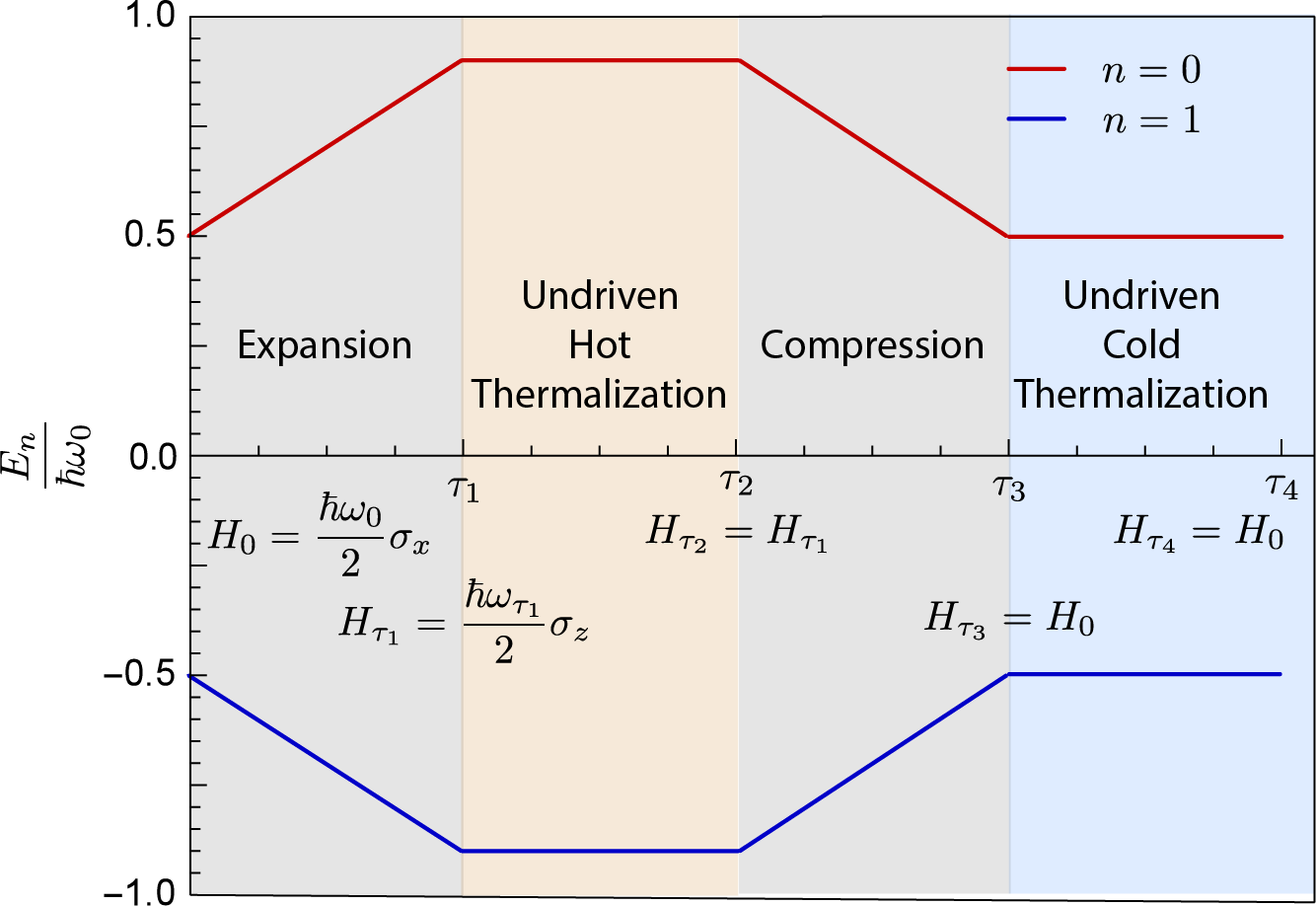
Figure A1: Change in the eigenenergies during one cycle. For $n=0$ [red upper line] and $n=1$ [blue lower line] the curves show the value of the instantaneous eigenenergies during one cycle. From the parameters considered in Sec. III, the relation between the initial and final frequencies is $\omega_{\tau_{1}}=1.8\times\omega_{0}$. With this information, we plotted the renormalized instantaneous eigenenergies $E_{n}\left(t\right)/\hbar\omega_{0}$ as a function of time. Additionally, we depicted each stroke as well as represented the Hamiltonian at the four key instants of time.

Appendix B Entropy Production

Efficiency and entropy production

Since the working substance ends up in the same initial state as the engine cycle due to the complete thermalization with the cold heat reservoir, the total change in energy and entropy are

$$\left\langle W_{1}\right\rangle+\left\langle W_{3}\right\rangle+\left\langle Q_{\text{h}}\right\rangle+\left\langle Q_{\text{c}}\right\rangle=0$$ (B1)

and

$$\Delta S_{2}+\Delta S_{4}=0,$$ (B2)

respectively. In Eq. (B2), $\Delta S_{4}=S\left(\rho_{0}^{\text{eq,c}}\right)-S\left(\rho_{\tau_{3}}\right)$ and $\Delta S_{2}=S\left(\rho_{\tau_{2}}\right)-S\left(\rho_{\tau_{1}}\right)$ are the changes in entropy during the fourth and second strokes, respectively. The first and third strokes are unitary and hence do not change the entropy. These equations express the conservation of energy and entropy in one cycle.

The total change of entropy of the working substance is equal to the total entropy production plus the total heat flux. Since the working substance interacts with two heat reservoirs, it contains two contributions to the heat flux, namely, $\beta_{\text{c}}\left\langle Q_{\text{c}}\right\rangle$ and $\beta_{\text{h}}\left\langle Q_{\text{h}}\right\rangle$. Therefore,

$$\Delta S_{\text{total}}=\left\langle\Sigma_{\text{total}}\right\rangle+\beta_{\text{h}}\left\langle Q_{\text{h}}\right\rangle+\beta_{\text{c}}\left\langle Q_{\text{c}}\right\rangle.$$ (B3)

From entropy conservation $\Delta S_{\text{total}}=0$, implying that the total amount of entropy produced is dispersed to the reservoirs.

The engine efficiency is given by

$$\eta=\frac{-\left\langle W_{1}\right\rangle-\left\langle W_{3}\right\rangle}{\left\langle Q_{\text{h}}\right\rangle}=1+\frac{\beta_{\text{c}}\left\langle Q_{\text{c}}\right\rangle}{\beta_{\text{c}}\left\langle Q_{\text{h}}\right\rangle},$$ (B4)

where Eq. (B1) has been employed and $\beta_{\text{c}}$ has been conveniently introduced. Substituting $\beta_{\text{c}}\left\langle Q_{\text{c}}\right\rangle$ from Eq. (B3) into Eq. (B4) and rearranging the terms one obtains

$$\eta=\eta_{\text{Carnot}}-\frac{\left\langle\Sigma_{\text{total}}\right\rangle}{\beta_{\text{c}}\left\langle Q_{\text{h}}\right\rangle}$$ (B5)

which is Eq. (3).

Entropy production and thermal divergences

In this subsection, we derive the expression for the total entropy production as a function of the thermal divergences [Eq. (4)]. We begin with Eq. (B4)

$$\eta=1+\frac{\left\langle Q_{\text{c}}\right\rangle}{\left\langle Q_{\text{h}}\right\rangle}=1+\frac{\mathcal{E}_{0}-\mathcal{E}_{\tau_{3}}}{\left\langle Q_{\text{h}}\right\rangle},$$ (B6)

where in the last equality we wrote the cold heat in terms of the internal energies.

Next, we use the following relation valid for the thermal divergence (see the Supplemental Material of Ref. Camati2016 for a quick derivation). Let $\rho_{t}$ be an arbitrary state in some time $t$ with Hamiltonian $H\left(t\right)$ and $\rho_{t}^{\text{eq}}$ an associated Gibbs state with same Hamiltonian and some reference inverse temperature $\beta$; then

$$D\left(\rho_{t}||\rho_{t}^{\text{eq}}\right)=\beta\left[\mathcal{E}\left(\rho_{t}\right)-F_{t}^{\text{eq}}\right]-S\left(\rho_{t}\right),$$ (B7)

where $F_{t}^{\text{eq}}=-\left(\beta\right)^{-1}\ln Z_{t}$ is the associated free energy and $Z_{t}=\text{Tr}\left[e^{-\beta H_{t}}\right]$ is the associated partition function.

We substitute the internal energies in the efficiency using the expressions

$$\beta_{\text{c}}\mathcal{E}\left(\rho_{0}^{\text{eq,c}}\right)=D\left(\rho_{0}^{\text{eq,c}}||\rho_{0}^{\text{eq,c}}\right)+S\left(\rho_{0}^{\text{eq,c}}\right)+\beta_{\text{c}}F_{0}^{\text{eq,c}}$$ (B8)

and

$$\beta_{\text{c}}\mathcal{E}\left(\rho_{\tau_{3}}\right)=D\left(\rho_{\tau_{3}}||\rho_{0}^{\text{eq,c}}\right)+S\left(\rho_{\tau_{3}}\right)+\beta_{\text{c}}F_{0}^{\text{eq,c}},$$ (B9)

where we have used $\rho_{\tau_{3}}^{\text{eq,c}}=\rho_{0}^{\text{eq,c}}$, and $F_{\tau_{3}}^{\text{eq,c}}=F_{0}^{\text{eq,c}}$ because the Hamiltonian is the same at times $\tau_{3}$ and zero (see Fig. A1). Hence,

$$\eta=1+\frac{\Delta S_{4}-D\left(\rho_{\tau_{3}}||\rho_{0}^{\text{eq,c}}\right)}{\beta_{\text{c}}\left\langle Q_{\text{h}}\right\rangle}=1+\frac{-\Delta S_{2}-D\left(\rho_{\tau_{3}}||\rho_{0}^{\text{eq,c}}\right)}{\beta_{\text{c}}\left\langle Q_{\text{h}}\right\rangle},$$ (B10)

where we already canceled the free-energy terms and used Eq. (B2). Using Eq. (B7), we substitute the von Neumann entropies

$$S\left(\rho_{\tau_{1}}\right)=\beta_{\text{h}}\mathcal{E}\left(\rho_{\tau_{1}}\right)-\beta_{\text{h}}F_{\tau_{1}}^{\text{eq,h}}-D\left(\rho_{\tau_{1}}||\rho_{\tau_{1}}^{\text{eq,h}}\right)$$ (B11)

and

$$S\left(\rho_{\tau_{2}}\right)=\beta_{\text{h}}\mathcal{E}\left(\rho_{\tau_{2}}\right)-\beta_{\text{h}}F_{\tau_{1}}^{\text{eq,h}}-D\left(\rho_{\tau_{2}}||\rho_{\tau_{1}}^{\text{eq,h}}\right)$$ (B12)

in order to obtain

$$\Delta S_{2}=\beta_{\text{h}}\left\langle Q_{\text{h}}\right\rangle-D\left(\rho_{\tau_{2}}||\rho_{\tau_{1}}^{\text{eq,h}}\right)+D\left(\rho_{\tau_{1}}||\rho_{\tau_{1}}^{\text{eq,h}}\right),$$ (B13)

where we already used the fact that $\rho_{\tau_{2}}^{\text{eq,h}}=\rho_{\tau_{1}}^{\text{eq,h}}$, $F_{\tau_{2}}^{\text{eq,h}}=F_{\tau_{1}}^{\text{eq,h}}$, because the Hamiltonians are the same at times $\tau_{1}$ and $\tau_{2}$. Replacing Eq. (B13) into Eq. (B10) and rearranging the terms we obtain

$$\eta=\eta_{\text{Carnot}}-\frac{D\left(\rho_{\tau_{1}}||\rho_{\tau_{1}}^{\text{eq,h}}\right)-D\left(\rho_{\tau_{2}}||\rho_{\tau_{1}}^{\text{eq,h}}\right)+D\left(\rho_{\tau_{3}}||\rho_{0}^{\text{eq,c}}\right)}{\beta_{\text{c}}\left\langle Q_{\text{h}}\right\rangle}.$$ (B14)

Comparing this equation to the efficiency in Eq. (B5), one obtains

$$\left\langle\Sigma_{\text{total}}\right\rangle=D\left(\rho_{\tau_{1}}||\rho_{\tau_{1}}^{\text{eq,h}}\right)-D\left(\rho_{\tau_{2}}||\rho_{\tau_{1}}^{\text{eq,h}}\right)+D\left(\rho_{\tau_{3}}||\rho_{0}^{\text{eq,c}}\right),$$ (B15)

which is Eq. (4).

Appendix C The quasistatic divergences

Before we demonstrate the expression for the quantum friction $\mathcal{F}$ we need to obtain an expression for the quasistatic divergence similar to Eq. (B7) for the thermal divergence.

In the first stroke, the initial state is always the cold Gibbs state $\rho_{0}^{\text{eq,c}}=e^{-\beta_{\text{c}}H_{0}}/Z_{0}^{\text{c}}=\sum_{n}p_{n}^{\text{eq,c},0}\Ket{E_{n}^{0}}\Bra{E_{n}^{0}}$, where $p_{n}^{\text{eq,c},0}$ are the respective Boltzmann weights. The the reference state for the first-stroke quasistatic divergence is

$$\rho_{\tau_{1}}^{\text{qs,c}}=\sum_{n}p_{n}^{\text{eq,c},0}\Ket{E_{n}^{\tau_{1}}}\Bra{E_{n}^{\tau_{1}}},$$ (C1)

where the eigenstates changed without changing the populations of the state. The quasistatic divergence is given by

$$D\left(\rho_{\tau_{1}}||\rho_{\tau_{1}}^{\text{qs,c}}\right)=-\text{Tr}\left[\rho_{\tau_{1}}\ln\rho_{\tau_{1}}^{\text{qs,c}}\right]-S\left(\rho_{\tau_{1}}\right).$$ (C2)

Expanding the trace in the basis of $H_{\tau_{1}}$ and using $\ln p_{n}^{\text{eq,c},0}=-\beta_{\text{c}}\left(E_{n}^{0}-F_{0}^{\text{eq,c}}\right)$ the first term of the divergence can be written as

$$-\text{Tr}\left[\rho_{\tau_{1}}\ln\rho_{\tau_{1}}^{\text{qs,c}}\right]=\sum_{n}\beta_{\text{c}}E_{n}^{0}\text{Tr}\left[\rho_{\tau_{1}}\Ket{E_{n}^{\tau_{1}}}\Bra{E_{n}^{\tau_{1}}}\right]-\beta_{\text{c}}F_{0}^{\text{eq,c}}.$$ (C3)

Now comes an important assumption that constrains the derivation. We assume that the ratio $E_{n}^{\tau_{1}}/E_{n}^{0}$ for every $n$ between the final and initial energies is constant. This applies at least for a qubit or a harmonic oscillator. In our case, we are considering a qubit working substance, so this ratio is $E_{n}^{\tau_{1}}/E_{n}^{0}=\omega_{\tau_{1}}/\omega_{0}$ for $n=0,1$. We multiply the term $E_{n}^{0}$ by $E_{n}^{\tau_{1}}/E_{n}^{\tau_{1}}=1$ and rearrange the eigenenergies $E_{n}^{\tau_{1}}$ inside the trace, obtaining the spectral decomposition of the final Hamiltonian $H_{\tau_{1}}=\sum_{n}E_{n}^{0}\Ket{E_{n}^{\tau_{1}}}\Bra{E_{n}^{\tau_{1}}}$. Therefore, we obtain the following expression for quasistatic divergence

$$D\left(\rho_{\tau_{1}}||\rho_{\tau_{1}}^{\text{qs,c}}\right)=\beta_{\text{c}}\frac{\omega_{0}}{\omega_{\tau_{1}}}\mathcal{E}\left(\rho_{\tau_{1}}\right)-\beta_{\text{c}}F_{0}^{\text{eq,c}}-S\left(\rho_{\tau_{1}}\right),$$ (C4)

which is the relation we were seeking.

Now, we want to obtain the same relation for the third stroke. However, the initial state is not the Gibbs state, in general, since an incomplete thermalization is performed. As we mentioned in the main text, the quasistatic state that would be obtained if we performed the compression stroke quasistatically is not the reference state used in the quasistatic divergence. Instead, we use the reference state $\rho_{\tau_{3}}^{\text{qs,h}}$, which is the quasistatic state that would have been obtained if the transformation was performed quasistatically and the initial state was the hot Gibbs state $\rho_{\tau_{2}}^{\text{eq,h}}=\sum_{n}p_{n}^{\text{eq,h},\tau_{1}}\Ket{E_{n}^{\tau_{1}}}\Bra{E_{n}^{\tau_{1}}}$. Hence,

$$\rho_{\tau_{3}}^{\text{qs,h}}=\sum_{n}p_{n}^{\text{eq,h},\tau_{1}}\Ket{E_{n}^{0}}\Bra{E_{n}^{0}}.$$ (C5)

The quasistatic divergence we use is

$$D\left(\rho_{\tau_{3}}||\rho_{\tau_{3}}^{\text{qs,h}}\right)=-\text{Tr}\left[\rho_{\tau_{3}}\ln\rho_{\tau_{3}}^{\text{qs,h}}\right]-S\left(\rho_{\tau_{3}}\right).$$ (C6)

Using the same strategy as before to calculate the first term we obtain

$$-\text{Tr}\left[\rho_{\tau_{3}}\ln\rho_{\tau_{3}}^{\text{qs,h}}\right]=\beta_{\text{h}}\frac{\omega_{\tau_{1}}}{\omega_{0}}\mathcal{E}\left(\rho_{\tau_{3}}\right)-\beta_{\text{h}}F_{\tau_{1}}^{\text{eq,h}},$$ (C7)

where we used $\ln p_{n}^{\text{eq,h},\tau_{1}}=-\beta_{\text{h}}\left(E_{n}^{\tau_{1}}-F_{\tau_{1}}^{\text{eq,h}}\right)$ and the spectral decomposition of the initial Hamiltonian is $H_{0}=\sum_{n}E_{n}^{0}\Ket{E_{n}^{0}}\Bra{E_{n}^{0}}$. Therefore, the relation we seek is

$$D\left(\rho_{\tau_{3}}||\rho_{\tau_{3}}^{\text{qs,h}}\right)=\beta_{\text{h}}\frac{\omega_{\tau_{1}}}{\omega_{0}}\mathcal{E}\left(\rho_{\tau_{3}}\right)-\beta_{\text{h}}F_{\tau_{1}}^{\text{eq,h}}-S\left(\rho_{\tau_{3}}\right).$$ (C8)

Appendix D Quantum Friction

Using Eqs. (C4) and (C8), we can derive the expression for the quantum friction. We begin the derivation from Eq. (B6) for the efficiency

$$\eta=1+\frac{\beta_{\text{c}}\mathcal{E}_{0}-\beta_{\text{c}}\mathcal{E}_{\tau_{3}}}{\beta_{\text{c}}\left\langle Q_{\text{h}}\right\rangle},$$ (D1)

where we multiplied the second term by $1=\beta_{\text{c}}/\beta_{\text{c}}$. Let us consider the numerator in the second term. We want to relate the initial energy to the quasistatic divergence. We use the expression of the quasistatic divergence given by Eq. (C4), $S\left(\rho_{\tau_{1}}\right)=S\left(\rho_{0}^{\text{eq,c}}\right)$ because the first stroke is unitary, and the identity $S\left(\rho_{0}^{\text{eq,c}}\right)=\beta_{\text{c}}\mathcal{E}\left(\rho_{0}^{\text{eq,c}}\right)-\beta_{\text{c}}F_{0}^{\text{eq,c}}$. Therefore, we can obtain the relation

$$\beta_{\text{c}}\mathcal{E}\left(\rho_{0}^{\text{eq,c}}\right)=\beta_{\text{c}}\frac{\omega_{0}}{\omega_{\tau_{1}}}\mathcal{E}\left(\rho_{\tau_{1}}\right)-D\left(\rho_{\tau_{1}}||\rho_{\tau_{1}}^{\text{qs,c}}\right),$$ (D2)

where we have isolated the initial energy. Equation (C8) already relates the internal energy $\mathcal{E}_{\tau_{3}}$ to the quasistatic divergence. However, to derive the desired expression we must eliminate the von Neumann entropy $S\left(\rho_{\tau_{3}}\right)$ from the equation. We do this by first using $S\left(\rho_{\tau_{3}}\right)=S\left(\rho_{\tau_{2}}\right)$, since the third stroke is unitary, and then using the relation for the thermal divergence Eq. (B7). Hence, we obtain

$$\beta_{\text{c}}\mathcal{E}\left(\rho_{\tau_{3}}\right)= \frac{\beta_{\text{c}}\omega_{0}}{\beta_{\text{h}}\omega_{\tau_{1}}}\left[D\left(\rho_{\tau_{3}}||\rho_{\tau_{3}}^{\text{qs,h}}\right)-D\left(\rho_{\tau_{2}}||\rho_{\tau_{1}}^{\text{eq,h}}\right)\right]$$

$$+\beta_{\text{c}}\frac{\omega_{0}}{\omega_{\tau_{1}}}\mathcal{E}\left(\rho_{\tau_{2}}\right),$$ (D3)

where we have already isolated the internal energy $\mathcal{E}_{\tau_{3}}$. Substituting Eqs. (D2) and (D3) into Eq. (D1), and manipulating the terms we arrive at

$$\eta=\eta_{\text{Otto}}-\frac{\mathcal{F}}{\beta_{\text{c}}\left\langle Q_{\text{h}}\right\rangle},$$ (D4)

which is Eq. (9), and we identify

$$\mathcal{F}=D\left(\rho_{\tau_{1}}||\rho_{\tau_{1}}^{\text{qs,c}}\right)+\frac{\omega_{0}\beta_{\text{c}}}{\omega_{\tau_{1}}\beta_{\text{h}}}\left[D\left(\rho_{\tau_{3}}||\rho_{\tau_{3}}^{\text{qs,h}}\right)-D\left(\rho_{\tau_{2}}||\rho_{\tau_{2}}^{\text{eq,h}}\right)\right]$$ (D5)

as the quantum friction [Eq. (10)].

Appendix E Interference Energy Contribution

In this appendix, we demonstrate the energy contribution due to the interference effect given by Eq. (19). This energy contribution comes, in fact, from the internal energy at $t=\tau_{3}$. This internal energy is given by $\mathcal{E}_{\tau_{3}}=\mathcal{E}\left(\rho_{\tau_{3}}\right)=\text{Tr}\left[\rho_{\tau_{3}}H_{0}\right]$. Let $\rho_{\tau_{2}}=\sum_{nm}\rho_{nm}\left(\tau_{2}\right)\Ket{E_{n}^{\tau_{1}}}\Bra{E_{m}^{\tau_{1}}}$ denote the state at the end of the second stroke, where $\rho_{nm}\left(\tau_{2}\right)=\Bra{E_{n}^{\tau_{1}}}\rho_{\tau_{2}}\Ket{E_{m}^{\tau_{1}}}$. The term $\rho_{10}\left(\tau_{2}\right)$ is given by Eq. (A13). The internal energy can be decomposed as

$$\mathcal{E}_{\tau_{3}}=\sum_{mm^{\prime}}\rho_{mm^{\prime}}\left(\tau_{2}\right)\sum_{n}E_{n}^{0}a_{nm}^{\text{com}}\left(\tau_{3},\tau_{2}\right)a_{nm^{\prime}}^{\text{com}*}\left(\tau_{3},\tau_{2}\right),$$ (E1)

where we used the spectral decomposition of the initial Hamiltonian, used $\rho_{\tau_{3}}=V_{\tau_{3},\tau_{2}}\rho_{\tau_{2}}V_{\tau_{3},\tau_{2}}^{\dagger}$, opened the trace, and used the definition of the energy transition amplitude defined in the main text. Splitting the summation $\sum_{m,m^{\prime}}=\sum_{m}+\sum_{m\neq m^{\prime}}$, the second term will be the interference contribution

$$\mathcal{E}_{\text{trans}}=\sum_{m\neq m^{\prime}}\rho_{mm^{\prime}}\left(\tau_{2}\right)\sum_{n}E_{n}^{0}a_{nm}^{\text{com}}\left(\tau_{3},\tau_{2}\right)a_{nm^{\prime}}^{\text{com}*}\left(\tau_{3},\tau_{2}\right).$$ (E2)

Writing the sum over $m$ and $m^{\prime}$ explicitly, one finds that the terms are the complex conjugates of each other. Hence,

$$\mathcal{E}_{\text{trans}}=2\sum_{n}E_{n}^{0}\text{Re}\left\{\rho_{10}\left(\tau_{2}\right)a_{n1}^{\text{com}}\left(\tau_{3},\tau_{2}\right)a_{n0}^{\text{com}*}\left(\tau_{3},\tau_{2}\right)\right\}.$$ (E3)

Using Eq. (A13) we finally arrive at

$$\mathcal{E}_{\text{trans}}= 2\sum_{n}E_{n}^{0}e^{-\gamma\tau_{\text{therm}}^{\text{h}}/2}$$

$$\times\text{Re}\left\{\rho_{10}\left(\tau_{1}\right)e^{+i\tau_{2}\omega_{\tau_{1}}\tau_{\text{therm}}^{\text{h}}}a_{n0}^{\text{com}}a_{n1}^{\text{com}*}\right\},$$ (E4)

where $\rho_{10}\left(\tau_{1}\right)=\Bra{E_{1}^{\tau_{1}}}\rho_{\tau_{1}}\Ket{E_{0}^{\tau_{1}}}$.

References

- (1) M. Esposito, Nonequilibrium fluctuations, fluctuation theorems, and counting statistics in quantum systems, Rev. Mod. Phys. 81, 1665 (2009).
- (2) Ronnie Kosloff , Quantum Thermodynamics: A Dynamical Viewpoint, Entropy 15, 2100 (2013).
- (3) S. Vinjanampathy and J. Anders, Quantum thermodynamics, Contemp. Phys. 57, 545 (2016).
- (4) J. Millen and A. Xuereb, Perspective on quantum thermodynamics, New J. Phys. 18, 011002 (2016).
- (5) R. Alicki and R. Kosloff, Introduction to Quantum Thermodynamics: History and Prospects, arXiv:1801.08314 (2018).
- (6) D. Gelbwaser-Klimovsky, W. Niedenzu, and G. Kurizki, Thermodynamics of quantum systems under dynamical control, Adv. At. Mol. Opt. Phys. 64, 329 (2015).
- (7) J. Roßnagel, S. T. Dawkins, K. N. Tolazzi, O. Abah, E. Lutz, F. Schmidt-Kaler, K. Singer, A single-atom heat engine, Science 352, 325 (2016).
- (8) G. Maslennikov, S. Ding, R. Hablutzel, J. Gan, A. Roulet, S. Nimmrichter, J. Dai, V. Scarani, D. Matsukevich, Quantum absorption refrigerator with trapped ions, Nat. Comm. 10, 202 (2019).
- (9) J. Klaers, S. Faelt, A. Imamoglu, and E. Togan, Squeezed Thermal Reservoirs as a Resource for a Nanomechanical Engine beyond the Carnot Limit, Phys. Rev. X 7, 031044 (2017).
- (10) J. P. S. Peterson, T. B. Batalhão, M. Herrera, A. M. Souza, R. S. Sarthour, I. S. Oliveira, R. M. Serra, Experimental characterization of a spin quantum heat engine, arXiv:1803.06021 (2018).
- (11) J. Klatzow, J. N. Becker, P. M. Ledingham, C. Weinzetl, K. T. Kaczmarek, D. J. Saunders, J. Nunn, I. A. Walmsley, R. Uzdin, E. Poem, Experimental Demonstration of Quantum Effects in the Operation of Microscopic Heat Engines, Phys. Rev. Lett. 122, 110601 (2019).
- (12) J. Aberg, Quantifying Superposition, arXiv:quant-ph/0612146 (2006).
- (13) T. Baumgratz, M. Cramer, and M. B. Plenio, Quantifying Coherence, Phys. Rev. Lett. 113, 140401 (2014).
- (14) A. Streltsov, G. Adesso, and M. B. Plenio, Colloquium: Quantum coherence as a resource, Rev. Mod. Phys. 89, 041003 (2017).
- (15) A. Winter and D. Yang, Operational Resource Theory of Coherence, Phys. Rev. Lett. 116, 120404 (2016).
- (16) U. Singh, M. N. Bera, A. Misra, A. K. Pati, Erasing Quantum Coherence: An Operational Approach, arXiv:1506.08186 (2017).
- (17) M. O. Scully, M. S. Zubairy, G. S. Agarwal, H. Walther, Extracting Work from a Single Heat Bath via Vanishing Quantum Coherence, Science 299, 862 (2003).
- (18) H. E. D. Scovil and E. O. Schulz-DuBois, Three-Level Masers as Heat Engines, Phys. Rev. Lett. 2, 262 (1959).
- (19) J. E. Geusic, E. O. Schulz-DuBios, and H. E. D. Scovil, Quantum Equivalent of the Carnot Cycle, Phys. Rev. 156, 343 (1967).
- (20) M. O. Scully, Quantum Photocell: Using Quantum Coherence to Reduce Radiative Recombination and Increase Efficiency, Phys. Rev. Lett. 104, 207701 (2010).
- (21) M. O. Scully, K. R. Chapin, K. E. Dorfman, M. B. Kim, and A. Svidzinsky, Quantum heat engine power can be increased by noise-induced coherence, PNAS 108, 15097 (2011).
- (22) K. E. Dorfman, M. B. Kim, and A. A. Svidzinsky, Increasing photocell power by quantum coherence induced by external source, Phys. Rev. A 84, 053829 (2011).
- (23) S. Rahav, U. Harbola, and S. Mukamel, Heat fluctuations and coherences in a quantum heat engine, Phys. Rev. A 86, 043843 (2012).
- (24) K. E. Dorfman, D. V. Voronine, S. Mukamel, and M. O. Scully, Photosynthetic reaction center as a quantum heat engine, PNAS 110, 2746 (2013).
- (25) H. P. Goswami and U. Harbola, Thermodynamics of quantum heat engines, Phys. Rev. A 88, 013842 (2013).
- (26) R. Uzdin, A. Levy, and R. Kosloff, Equivalence of Quantum Heat Machines, and Quantum-Thermodynamic Signatures, Phys. Rev. X 5, 031044 (2015).
- (27) D. Türkpençe and Ö. E. Müstecaplıoğlu, Quantum fuel with multilevel atomic coherence for ultrahigh specific work in a photonic Carnot engine, Phys. Rev. E 93, 012145 (2016).
- (28) R. Uzdin, Coherence-Induced Reversibility and Collective Operation of Quantum Heat Machines via Coherence Recycling, Phys. Rev. Applied 6, 024004 (2016).
- (29) K. E. Dorfman, D. Xu, and J. Cao, Efficiency at maximum power of a laser quantum heat engine enhanced by noise-induced coherence, Phys. Rev. E 97, 042120 (2018).
- (30) K. Brandner, M. Bauer, and U. Seifert, Universal Coherence-Induced Power Losses of Quantum Heat Engines in Linear Response, Phys. Rev. Lett. 119, 170602 (2017).
- (31) A. V. Dodonov, D. Valente, T. Werlang, Quantum power boost in a nonstationary cavity-QED quantum heat engine, J. Phys. A: Math. Theor. 51, 365302 (2018).
- (32) I. Marvian, Coherence distillation machines are impossible in quantum thermodynamics, arXiv:1805.01989 (2018).
- (33) R. Kosloff and Y. Rezek, The Quantum Harmonic Otto Cycle, Entropy 19, 136 (2017).
- (34) S. R. de Groot and P. Mazur, Non-Equilibrium Thermodynamics, (Dover Publications, Inc., New York, 1984).
- (35) G. Lebon, D. Jou, and J. Casas-Vázques, Understading Non-Equilibrium Thermodynamics: Foundations, Applications, Frontiers, (Springer-Verlag, Berlin, 2008).
- (36) Y. A. Çengel and M. A. Boles, Thermodynamics An Engineering Approach 8th edition (McGraw-Hill Education, New York, 2015).
- (37) Y. Rezek, Reflections on Friction in Quantum Mechanics, Entropy 12, 1885 (2010).
- (38) R. Kosloff and T. Feldmann, Discrete four-stroke quantum heat engine exploring the origin of friction, Phys. Rev. E 65, 055102(R) (2002).
- (39) T. Feldmann and R. Kosloff, Quantum four-stroke heat engine: Thermodynamic observables in a model with intrinsic friction, Phys. Rev. E 68, 016101 (2003).
- (40) T. Feldmann and R. Kosloff, Characteristics of the limit cycle of a reciprocating quantum heat engine, Phys. Rev. E 70, 046110 (2004).
- (41) T. Feldmann and R. Kosloff, Quantum lubrication: Suppression of friction in a first-principles four-stroke heat engine, Phys. Rev. E 73, 025107(R) (2006).
- (42) Y. Rezek and R. Kosloff, Irreversible performance of a quantum harmonic heat engine, New J. Phys. 8, 83 (2006).
- (43) T. Feldmann and R. Kosloff, Short time cycles of purely quantum refrigerators, Phys. Rev. E 85, 051114 (2012).
- (44) A. M. Zagoskin, S. Savel’ev, Franco Nori, and F. V. Kusmartsev, Squeezing as the source of inefficiency in the quantum Otto cycle, Phys. Rev. B 86, 014501 (2012).
- (45) G. Thomas and R. S. Johal, Friction due to inhomogeneous driving of coupled spins in a quantum heat engine, Eur. Phys. J. B 87, 166 (2014).
- (46) F. Plastina, A. Alecce, T. J. G. Apollaro, G. Falcone, G. Francica, F. Galve, N. Lo Gullo, and R. Zambrini, Irreversible Work and Inner Friction in Quantum Thermodynamic Processes, Phys. Rev. Lett. 113, 260601 (2014).
- (47) A. Alecce, F. Galve, N. Lo Gullo, L. Dell’Anna, F. Plastina, and R. Zambrini, Quantum Otto cycle with inner friction: finite-time and disorder effects, New J. Phys. 17, 075007 (2015).
- (48) L. A. Correa, J. P. Palao, and D. Alonso, Internal dissipation and heat leaks in quantum thermodynamic cycles, Phys. Rev. E 92, 032136 (2015).
- (49) A. del Campo, A. Chenu, S. Deng, H. Wu, Friction-free quantum machines, In: F. Binder, L. A. Correa, C. Gogolin, J. Anders, and G. Adesso (eds.), Thermodynamics in the Quantum Regime (Springer, Cham, 2018).
- (50) E. Torrontegui, S. Ibáñez, S. Martínez-Garaot, M. Modugno, A. del Campo, D. Guéry-Odelin, A. Ruschhaupt, X. Chen, and J. G. Muga, Shortcuts to Adiabaticity, Adv. At. Mol. Opt. Phy. 62, 117 (2013).
- (51) A. del Campo, J. Goold, and M. Paternostro, More bang for your buck: Super-adiabatic quantum engines, Sci. Rep. 4, 6208 (2014).
- (52) K. Funo, J.-N. Zhang, C. Chatou, K. Kim, M. Ueda, and A. del Campo, Universal Work Fluctuations During Shortcuts to Adiabaticity by Counterdiabatic Driving, Phys. Rev. Lett. 118, 100602 (2017).
- (53) Y. Zheng, S. Campbell, G. De Chiara, and D. Poletti, Cost of counterdiabatic driving and work output, Phys. Rev. A 94, 042132 (2016).
- (54) S. Campbell and S. Deffner, Trade-Off Between Speed and Cost in Shortcuts to Adiabaticity, Phys. Rev. Lett. 118, 100601 (2017).
- (55) E. Calzetta, Not quite free shortcuts to adiabaticity, Phys. Rev. A 98, 032107 (2018).
- (56) J. P. Santos, L. C. Céleri, G. T. Landi, and M. Paternostro, The role of quantum coherence in non-equilibrium entropy production, npj Quantum Inf. 5, 23 (2019).
- (57) G. Francica, J. Goold, and F. Plastina, The role of coherence in the non-equilibrium thermodynamics of quantum systems, Phys. Rev. E 99, 042105 (2019).
- (58) T. B. Batalhão, A. M. Souza, L. Mazzola, R. Auccaise, R. S. Sarthour, I. S. Oliveira, J. Goold, G. De Chiara, M. Paternostro, and R. M. Serra, Experimental Reconstruction of Work Distribution and Study of Fluctuation Relations in a Closed Quantum System, Phys. Rev. Lett. 113, 140601 (2014).
- (59) T. B. Batalhão, A. M. Souza, R. S. Sarthour, I. S. Oliveira, M. Paternostro, E. Lutz, and R. M. Serra, Irreversibility and the arrow of time in a quenched quantum system, Phys. Rev. Lett. 115, 190601 (2015).
- (60) P. A. Camati, J. P. S. Peterson, T. B. Batalhão, K. Micadei, A. M. Souza, R. S. Sarthour, I. S. Oliveira, and R. M. Serra, Experimental Rectification of Entropy Production by Maxwell’s Demon in a Quantum System, Phys. Rev. Lett. 117, 240502 (2016).
- (61) H. Wang, S. Liu, and J. He, Thermal entanglement in two-atom cavity QED and the entangled quantum Otto engine, Phys. Rev. E 79, 041113 (2009).
- (62) F. Altintas and Ö. E. Müstecaplıoğlu, General formalism of local thermodynamics with an example: Quantum Otto engine with a spin-1/2 coupled to an arbitrary spin, Phys. Rev. E 92, 022142 (2015).
- (63) H.-P. Breuer and F. Petruccione, The Theory of Open Quantum Systems (Oxford University Press, Inc., New York, 2003).
- (64) S. Chakraborty, P. Cherian J, S. Ghosh, On thermalization of two-level quantum systems, arXiv:1604.04998 (2016).
- (65) H. Umegaki, Conditional expectation in operator algebra I, Tohoku Math. J. 6, 177 (1954).
- (66) V. Vedral, The role of relative entropy in quantum information theory, Rev. Mod. Phys. 74, 197 (2002).
- (67) M. M. Wilde, Quantum Information Theory 2nd, (Cambridge University Press, Cambridge, 2017).
- (68) S. Deffner and E. Lutz, Nonequilibrium Entropy Production for Open Quantum Systems, Phys. Rev. Lett. 107, 140404 (2011).
- (69) M. Campisi and R. Fazio, Dissipation, correlation and lags in heat engines, J. Phys. A: Math. Theor. 49, 345002 (2016).
- (70) D. Janzing, Quantum Thermodynamics with Missing Reference Frames: Decompositions of Free Energy Into Non-Increasing Components, J. Stat. Phys. 125, 761 (2006).
- (71) M. Lostaglio, D. Jennings, and T. Rudolph, Description of quantum coherence in thermodynamic processes requires constraints beyond free energy, Nat. Comm. 6, 6383 (2015).
- (72) Marcela Herrera (private communications).
- (73) K. Micadei, J. P. S. Peterson, A. M. Souza, R. S. Sarthour, I. S. Oliveira, G T. Landi, T. B. Batalhão, R. M. Serra, and E. Lutz, Reversing the direction of heat flow using quantum correlations, Nat. Commun. 10, 2456 (2019).