Reciprocals and Flowers in Convexity

?abstractname?

We study new classes of convex bodies and star bodies with unusual properties. First we define the class of reciprocal bodies, which may be viewed as convex bodies of the form “$1/K$”. The map $K\mapsto K^{\prime}$ sending a body to its reciprocal is a duality on the class of reciprocal bodies, and we study its properties.

To connect this new map with the classic polarity we use another construction, associating to each convex body $K$ a star body which we call its flower and denote by $K^{\clubsuit}$. The mapping $K\mapsto K^{\clubsuit}$ is a bijection between the class $\mathcal{K}_{0}^{n}$ of convex bodies and the class $\mathcal{F}^{n}$ of flowers. Even though flowers are in general not convex, their study is very useful to the study of convex geometry. For example, we show that the polarity map $\circ:\mathcal{K}_{0}^{n}\to\mathcal{K}_{0}^{n}$ decomposes into two separate bijections: First our flower map $\clubsuit:\mathcal{K}_{0}^{n}\to\mathcal{F}^{n}$, followed by a slight modification $\Phi$ of the spherical inversion which maps $\mathcal{F}^{n}$ back to $\mathcal{K}_{0}^{n}$. Each of these maps has its own properties, which combine to create the various properties of the polarity map.

We study the various relations between the four maps $\prime$, $\circ$, $\clubsuit$ and $\Phi$ and use these relations to derive some of their properties. For example, we show that a convex body $K$ is a reciprocal body if and only if its flower $K^{\clubsuit}$ is convex.

We show that the class $\mathcal{F}^{n}$ has a very rich structure, and is closed under many operations, including the Minkowski addition. This structure has corollaries for the other maps which we study. For example, we show that if $K$ and $T$ are reciprocal bodies so is their “harmonic sum” $(K^{\circ}+T^{\circ})^{\circ}$. We also show that the volume $\left|\left(\sum_{i}\lambda_{i}K_{i}\right)^{\clubsuit}\right|$ is a homogeneous polynomial in the $\lambda_{i}$’s, whose coefficients can be called “$\clubsuit$-type mixed volumes”. These mixed volumes satisfy natural geometric inequalities, such as an elliptic Alexandrov-Fenchel inequality. More geometric inequalities are also derived.

1 Introduction

In this paper we study new classes of convex bodies and star bodies in $\mathbb{R}^{n}$ with some unusual properties. We will provide precise definitions below, but let us first describe the general program of what will follow.

One of our new classes, “reciprocal” bodies, may be viewed as bodies of the form “$\frac{1}{K}$” for a convex body $K$. They appear as the image of a new “quasi-duality” operation on the class $\mathcal{K}_{0}^{n}$ of convex bodies. We denote this new map by $K\mapsto K^{\prime}$. This operation reverses order (with respect to inclusions) and has the property $K^{\prime\prime\prime}=K^{\prime}$. Hence the map ^′ is indeed a duality on its image.

This new operation is connected to the classical operation of polarity $\circ:K\mapsto K^{\circ}$ via another construction, which we call simply the “flower” of a body $K$ and denote by $\clubsuit:K\mapsto K^{\clubsuit}$. We provide the definition of $K^{\clubsuit}$ in Definition 3 below, but an equivalent description which sheds light on the "flower" nomenclature is

$$K^{\clubsuit}=\bigcup\left\{B\left(\frac{x}{2},\frac{\left|x\right|}{2}\right):\ x\in K\right\}$$

(see Proposition 19). Here $B(y,r)$ is the Euclidean ball with center $y\in\mathbb{R}^{n}$ and radius $r\geq 0$. In other words, $K^{\clubsuit}$ is the union of all balls passing through the origin having diameter $[0,x]$ with $x\in K$.

In general, $K^{\clubsuit}$ is a star body which is not necessarily convex. The flower of a convex body was previously studied for very different reasons in the field of stochastic geometry – see Remark 7. We show that our new map ^′ is precisely $K^{\prime}=\left(K^{\clubsuit}\right)^{\circ}$. We also show that $K$ belongs to the image of ^′, i.e. $K$ is a reciprocal body, if and only if $K^{\clubsuit}$ is convex. This means that such reciprocal bodies are in some sense “more convex” than other convex bodies, and can also be thought of as “doubly convex” bodies.

Interestingly, the flower map $\clubsuit$ is also connected to the $n$-dimensional spherical inversion $\Phi$ when applied to star bodies ($\Phi$ is defined by applying the pointwise map $\mathcal{I}(x)=\frac{x}{\left|x\right|^{2}}$ and taking set complement – see Definition 11). We describe the class of convex bodies on which $\Phi$ preserves convexity.

The method of study of these questions looks novel and some of the results are not intuitive. Just as an example, we show that if $\Phi(A)$ and $\Phi(B)$ are convex (for some star bodies $A$ and $B$) then $\Phi(A+B)$ is convex as well, where $A+B$ is the Minkowski addition (see Corollary 37).

The family $\mathcal{F}^{n}$ of flowers should play a central role in the study of convexity. It has a very rich structure. For example, it is closed under the Minkowski addition, and is also preserved by orthogonal projections and sections. “Flower mixed volumes” also exist and, perhaps most interestingly, we have a decomposition of the classical polarity operation as

$$\mathcal{K}_{0}^{n}\stackrel{{\scriptstyle\clubsuit}}{{\longrightarrow}}\mathcal{F}^{n}\stackrel{{\scriptstyle\Phi}}{{\longrightarrow}}\mathcal{K}_{0}^{n}.$$

Here the maps $\clubsuit$ and $\Phi$ are $1$-1 and onto, and we have $\circ=\Phi\clubsuit$ in the sense that $K^{\circ}=\Phi\left(K^{\clubsuit}\right)$ for all $K\in\mathcal{K}_{0}^{n}$.

The class of reciprocal bodies also looks interesting. No polytope belongs to this class, and no centrally symmetric ellipsoids (besides Euclidean balls centered at $0$). At the same time this class is clearly important, as seen from its properties and the fact that it coincides with the “doubly convex” bodies. We provide several $2$-dimensional pictures to help create some intuition about this class of reciprocal bodies and about the class of flowers.

To make the above claims more precise, let us now give some basic definitions and fix our notation. The reader may consult [12] for more information. By a convex body in $\mathbb{R}^{n}$ we mean a set $K\subseteq\mathbb{R}^{n}$ which is closed and convex. We will always assume further that $0\in K$, but we do not assume that $K$ is compact or has non-empty interior. We denote the set of all such bodies by $\mathcal{K}_{0}^{n}$. The support function of $K$ is the function $h_{K}:S^{n-1}\to[0,\infty]$ defined by $h_{K}(\theta)=\sup_{x\in K}\left\langle x,\theta\right\rangle$. Here $S^{n-1}=\left\{\theta\in\mathbb{R}^{n}:\ \left|\theta\right|=1\right\}$ is the unit Euclidean sphere, and $\left\langle\cdot,\cdot\right\rangle$ is the standard scalar product on $\mathbb{R}^{n}$. The function $h_{K}$ uniquely defines the body $K$.

The Minkowski sum of two convex bodies is defined by

$$K+T=\overline{\left\{x+y:\ x\in K,\ y\in T\right\}}$$

(the closure is not needed if $K$ or $T$ is compact). The homothety operation is defined by $\lambda K=\left\{\lambda x:\ x\in K\right\}$. These operations are related to the support function by the identity $h_{\lambda K+T}=\lambda h_{K}+h_{T}$.

We say that $A\subseteq\mathbb{R}^{n}$ is a star set if $A$ is non-empty and $x\in A$ implies that $\lambda x\in A$ for all $0\leq\lambda\leq 1$. The radial function $r_{A}:S^{n-1}\to[0,\infty]$ of $A$ is defined by $r_{A}(\theta)=\sup\left\{\lambda\geq 0:\ \lambda\theta\in A\right\}$. For us, a star body is simply a star set which is radially closed, in the sense that $r_{A}(\theta)\theta\in A$ for all directions $\theta\in S^{n-1}$ satisfying $r_{A}(\theta)<\infty$. For such bodies $r_{A}$ uniquely defines $A$.

The polarity map $\circ:\mathcal{K}_{0}^{n}\to\mathcal{K}_{0}^{n}$ maps every body $K$ to its polar

$$K^{\circ}=\left\{y\in\mathbb{R}^{n}:\ \left\langle x,y\right\rangle\leq 1\text{ for all }x\in K\right\}.$$ (1.1)

It follows that $h_{K}=\frac{1}{r_{K^{\circ}}}$. The polarity map is a duality in the following sense:

• It is order reversing: If $K\subseteq T$ then $K^{\circ}\supseteq T^{\circ}$.

• It is an involution: $K^{\circ\circ}=K$ for all $K\in\mathcal{K}_{0}^{n}$ (if $A$ is only a star body, then $A^{\circ\circ}$ is the closed convex hull of $A$).

In fact, it was proved in [1] that the polarity map is essentially the only duality on $\mathcal{K}_{0}^{n}$. Similar results on different classes of convex bodies were proved earlier in [5] and [3].

The structure of a set equipped with a duality relation is common in mathematics. A basic example is the set $[0,\infty]$ equipped with the inversion $x\mapsto x^{-1}$ (we set of course $0^{-1}=\infty$ and $\infty^{-1}=0$). Following this analogy, one may think of $K^{\circ}$ as a certain inverse “$K^{-1}$”. This point of view can indeed be useful – see for example [10] and [7].

However, in recent works ([8], [9]), the authors discussed the application of functions such as $x\mapsto x^{\alpha}$ ($0\leq\alpha\leq 1$) and $x\mapsto\log x$ to convex bodies. Applying the same idea to the inversion $x\mapsto\frac{1}{x}$, we obtain a new notion of the reciprocal body “$K^{-1}$” . Recall that given a function $g:S^{n-1}\to[0,\infty]$, its Alexandrov body, or Wulff shape, is defined by

$$A\left[g\right]=\left\{x\in\mathbb{R}^{n}:\ \left\langle x,\theta\right\rangle\leq g(\theta)\text{ for all }\theta\in S^{n-1}\right\}.$$

In other words, $A\left[g\right]$ is the biggest convex body such that $h_{A[g]}\leq g$. In particular, for every convex body $K$ we have $K=A\left[h_{K}\right]$. We may now define:

Definition 1.

Given $K\in\mathcal{K}_{0}^{n}$, the reciprocal body $K^{\prime}\in\mathcal{K}_{0}^{n}$ is defined by $K^{\prime}=A\left[\frac{1}{h_{K}}\right].$

More explicitly, we have

$$K^{\prime}=\bigcap_{\theta\in S^{n-1}}H^{-}\left(\theta,h_{K}(\theta)^{-1}\right),$$

where $H^{-}(\theta,c)=\left\{x\in\mathbb{R}^{n}:\ \left\langle x,\theta\right\rangle\leq c\right\}.$

The idea of constructing new interesting convex bodies as Alexandrov bodies is not new. As one important recent example, Böröczky, Lutwak, Yang and Zhang consider in [2] the body $A\left[h_{K}^{1-\lambda}h_{L}^{\lambda}\right]$, which they call the $\lambda$-logarithmic mean of $K$ and $L$.

Figure 1.1 depicts some simple convex bodies in $\mathbb{R}^{2}$ and their reciprocal. Some basic properties of the reciprocal map $K\mapsto K^{\prime}$ are immediate from the definition:

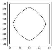
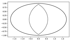
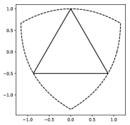
?figurename? 1.1: convex bodies (solid) and their reciprocals (dashed)

Proposition 2.

For all $K,T\in\mathcal{K}_{0}^{n}$ we have:

1. $K^{\prime}\subseteq K^{\circ}$, with an equality if and only if $K$ is a Euclidean ball.

2. If $K\supseteq T$ then $K^{\prime}\subseteq T^{\prime}$.

3. $K^{\prime\prime}\supseteq K$.

4. $K^{\prime\prime\prime}=K^{\prime}$.

?proofname? .

For (1), note that for every $\theta\in S^{n-1}$ we have $1=\left\langle\theta,\theta\right\rangle\leq h_{K}(\theta)h_{K^{\circ}}(\theta)$. Hence $K^{\circ}=A\left[h_{K^{\circ}}\right]\geq A\left[\frac{1}{h_{K}}\right]=K^{\prime}$. An equality $K^{\prime}=K^{\circ}$ implies that $h_{K^{\circ}}=\frac{1}{h_{K}}$, or equivalently $r_{K}=\frac{1}{h_{K^{\circ}}}=h_{K}$. This implies that $K$ is a ball.

Property (2) is obvious from the definition.

For property (3), we know that $h_{K^{\prime}}\leq\frac{1}{h_{K}}$ so $K^{\prime\prime}=A\left[\frac{1}{h_{K^{\prime}}}\right]\geq A\left[h_{K}\right]=K$.

Finally, (4) is a formal consequence of (2) and (3): We know that $K^{\prime\prime}\supseteq K$, so $K^{\prime\prime\prime}\subseteq K^{\prime}$. On the other hand applying (3) to $K^{\prime}$ gives $K^{\prime\prime\prime}\supseteq K^{\prime}$. ∎

Let us write

$${\cal R}^{n}=\left\{K^{\prime}:\ K\in\mathcal{K}_{0}^{n}\right\}.$$

Note that properties (2) and (4) above imply that ^′ is a duality on the class $\mathcal{R}^{n}$. Also note that $K\in\mathcal{R}^{n}$ if and only if $K^{\prime\prime}=K$.

Our next goal is to give an alternative description of the reciprocal body $K^{\prime}$. Towards this goal we define:

Definition 3.

1. For a convex body $K\in\mathcal{K}_{0}^{n}$ we denote by $K^{\clubsuit}$ the star body with radial function $r_{K^{\clubsuit}}=h_{K}$.

2. We say that a star body $A\subseteq\mathbb{R}^{n}$ is a flower if $A=\bigcup_{x\in C}B\left(\frac{x}{2},\frac{\left|x\right|}{2}\right)$, where $C\subseteq\mathbb{R}^{n}$ is some closed set. The class of all flowers in $\mathbb{R}^{n}$ is denoted by $\mathcal{F}^{n}$.

The two parts of the definition are related by the following:

Theorem 4.

For every $K\in\mathcal{K}_{0}^{n}$ we have $K^{\clubsuit}\in\mathcal{F}^{n}$. Moreover, the map $\clubsuit:\mathcal{K}_{0}^{n}\to\mathcal{F}^{n}$ is one to one and onto. Equivalently, every flower $A$ is of the form $A=K^{\clubsuit}$ for a unique $K\in\mathcal{K}_{0}^{n}$; We have $A=\bigcup_{x\in K}B\left(\frac{x}{2},\frac{\left|x\right|}{2}\right)$, and we simply say that $A$ is the flower of $K$.

This theorem is a combination of Proposition 17(2), Proposition 19, and Remark 21.

As we will see flowers play an important role in connecting the reciprocity map to the polarity map. Note that in general $K^{\clubsuit}$ is not convex. Figure 1.2 depicts the flowers of some convex bodies in $\mathbb{R}^{2}$. Another example that will be important in the sequel is the following:

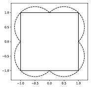
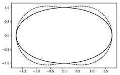
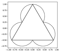
?figurename? 1.2: convex bodies (solid) and their flowers (dashed)

Example 5.

For $x\in\mathbb{R}^{n}$ write $[0,x]=\left\{\lambda x:\ 0\leq\lambda\leq 1\right\}$. Also denote the Euclidean ball with center $x$ and radius $r>0$ by $B(x,r)$, and write $B_{x}=B\left(\frac{x}{2},\frac{\left|x\right|}{2}\right)$. Then $[0,x]^{\clubsuit}=B_{x}$. Indeed, a direct computation gives

$$h_{[0,x]}(\theta)=r_{B_{x}}(\theta)=\max\left\{\left\langle x,\theta\right\rangle,0\right\}.$$

The identity $[0,x]^{\clubsuit}=B_{x}$ is also a classical theorem in geometry sometimes referred to as Thales’s theorem: If an interval $[a,b]\subseteq\mathbb{R}^{n}$ is a diameter of a ball $B$, then $\partial B$ is precisely the set of points $y$ such that $\measuredangle ayb=90^{\circ}$.

The polarity map, the reciprocal map and the flower are all related via the following formula:

Proposition 6.

For every $K\in\mathcal{K}_{0}^{n}$ we have $\left(K^{\clubsuit}\right)^{\circ}=K^{\prime}$.

Note that even though in general $K^{\clubsuit}\notin\mathcal{K}_{0}^{n}$, we may still compute its polar using (1.1).

?proofname?.

By definition $x\in\left(K^{\clubsuit}\right)^{\circ}$ if and only if $\left\langle x,y\right\rangle\leq 1$ for all $y\in K^{\clubsuit}$. It is obviously enough to check this for $y\in\partial K^{\clubsuit}$, i.e. $y=r_{K^{\clubsuit}}(\theta)\theta=h_{K}(\theta)\theta$ for some $\theta\in S^{n-1}$.

Hence $x\in\left(K^{\clubsuit}\right)^{\circ}$ if and only if for all $\theta\in S^{n-1}$ we have $\left\langle x,h_{K}(\theta)\theta\right\rangle\leq 1$, or $\left\langle x,\theta\right\rangle\leq\frac{1}{h_{K}(\theta)}$. This means that $x\in A\left[\frac{1}{h_{K}}\right]=K^{\prime}$. ∎

Remark 7.

The flower of a convex body was studied in stochastic geometry under the name “Voronoi Flower” (see e.g. [13]). The reason for the name is the following relation to Voronoi tessellations: For a discrete set of points $P\subseteq\mathbb{R}^{n}$, consider the (open) Voronoi cell

$$Z=\left\{x\in\mathbb{R}^{n}:\ \left|x-0\right|<\left|x-y\right|\text{ for all }y\in P\right\}.$$

Then for any convex body $K$ we have $Z\supseteq K$ if and only if $P\cap\left(2K^{\clubsuit}\right)=\emptyset$. It follows that if for example $P$ is chosen according to a homogeneous Poisson point process, then the probability that $Z\supseteq K$ is computable from the volume of $K^{\clubsuit}$.

In Section 2 we discuss basic properties of the flower map $\clubsuit$ and prove representation formulas for both $K^{\clubsuit}$ and $K^{\prime}$. We also study the pre-images of a body $K\in\mathcal{R}^{n}$ under the reciprocity map. Since $\prime$ is not a duality on all of $\mathcal{K}_{0}^{n}$, the set of pre-images

$$\left\{A\in\mathcal{K}_{0}^{n}:\ A^{\prime}=K\right\}$$

may in general contain more than one body. We study this set, and prove the following results:

Theorem 8.

1. If $K\in\mathcal{R}^{n}$ is a smooth convex body then $K=A^{\prime}$ for a unique $A\in\mathcal{K}_{0}^{n}$.

2. For a general $K\in\mathcal{R}^{n}$, the set $\left\{A\in\mathcal{K}_{0}^{n}:\ A^{\prime}=K\right\}$ is a convex subset of $\mathcal{K}_{0}^{n}$.

The main goal of Section 3 is to prove the following theorem, characterizing the class $\mathcal{R}^{n}$ of reciprocal bodies:

Theorem 9.

$K\in\mathcal{R}^{n}$ if and only if $K^{\clubsuit}$ is convex.

As a corollary we obtain:

Corollary 10.

For every $K\in\mathcal{R}^{n}$ and every subspace $E\subseteq\mathbb{R}^{n}$ one has $\left(\operatorname{Proj}_{E}K\right)^{\prime}=\operatorname{Proj}_{E}K^{\prime}$, where $\operatorname{Proj}_{E}$ denotes the orthogonal projection onto $E$.

We will prove Theorem 9 by connecting the various maps we constructed so far with another duality on the class of star-bodies:

Definition 11.

1. Let $\mathcal{\mathcal{I}}:\mathbb{R}^{n}\setminus\left\{0\right\}\to\mathbb{R}^{n}\setminus\left\{0\right\}$ denote the spherical inversion $\mathcal{\mathcal{I}}(x)=\frac{x}{\left|x\right|^{2}}$.

2. Given a star body $A$, we denote by $\Phi(A)$ the star body with radial function $r_{\Phi(A)}=\frac{1}{r_{A}}$.

The map $A\mapsto\Phi(A)$ is obviously a duality on the class of star bodies. It is sometimes called star duality and denoted by $A^{\ast}$ (see [11]), but we will prefer the notation $\Phi(A)$. Note that $\Phi$ is “essentially the same” as the pointwise map $\mathcal{I}$ in the sense that $\partial\Phi(A)=\mathcal{I}\left(\partial A\right)$, but $\mathcal{I}$ maps the interior of $A$ to the exterior of $\Phi(A)$ and vice versa. Here by the boundary $\partial A$ of a star body $A$ we mean

$$\partial A=\left\{r_{A}(\theta)\theta:\ \theta\in S^{n-1}\text{ such that }0<r_{A}(\theta)<\infty\right\}.$$

One interesting relation between $\Phi$ and our previous definitions is the following (see Propositions 28(2) and 33):

Theorem 12.

$\Phi$ is a bijection between $\mathcal{K}_{0}^{n}$ and $\mathcal{F}^{n}$. Moreover, the polarity map decomposes as

$$\circ:\mathcal{K}_{0}^{n}\stackrel{{\scriptstyle\clubsuit}}{{\longrightarrow}}\mathcal{F}^{n}\stackrel{{\scriptstyle\Phi}}{{\longrightarrow}}\mathcal{K}_{0}^{n},$$

in the sense that $\Phi\left(K^{\clubsuit}\right)=K^{\circ}$ for all $K\in\mathcal{K}_{0}^{n}$.

In Section 4 we use the results of Section 3 to further study the class of flowers, with applications to the study of reciprocity and the map $\Phi$. First we understand when the map $\Phi$ preserves convexity. By Theorem 12, as $\Phi$ is an involution, we know that $\Phi(A)$ is convex if and only if $A$ is a flower. When $A$ is in addition convex, we have:

Theorem 13.

If $K\in\mathcal{K}_{0}^{n}$ then $\Phi(K)$ is convex if and only if $K^{\circ}\in\mathcal{R}^{n}$.

(See Proposition 33). We then show that the class $\mathcal{F}^{n}$ has a lot of structure:

Theorem 14.

Fix $A,B\in\mathcal{F}^{n}$ and a linear subspace $E\subseteq\mathbb{R}^{n}$. Then $A+B$ and $\operatorname{conv}A$ are flowers in $\mathbb{R}^{n}$, and $A\cap E$ and $\operatorname{Proj}_{E}A$ are flowers in $E$.

(See Propositions 35, 39 and 40). As corollaries we obtain:

Corollary 15.

1. If $K,T\in\mathcal{R}^{n}$ then $\left(K^{\circ}+T^{\circ}\right)^{\circ}\in\mathcal{R}^{n}$.

2. If $K,T$ are convex bodies then $\Phi\left(\Phi(K)+\Phi(T)\right)$ is also convex.

As another corollary we construct a new addition $\oplus$ on $\mathcal{K}_{0}^{n}$ such that the class $\mathcal{R}^{n}$ is closed under $\oplus$. Moreover, when restricted to $\mathcal{R}^{n}$, this new addition has all properties one may expect: it is associative, commutative and monotone, it has $\left\{0\right\}$ as an identity element, and it satisfies $\lambda K\oplus\mu K=\left(\lambda+\mu\right)K$.

The final Section 5 is devoted to the study of inequalities. We begin by showing that the maps $\clubsuit,\Phi$ and $\prime$ are all convex in appropriate senses. We also study the functional $K\mapsto\left|K^{\clubsuit}\right|$, where $\left|\cdot\right|$ denotes the volume. We prove results that are analogous to Minkowski’s theorem of polynomiality of volume and to the Alexandrov-Fenchel inequality:

Theorem 16.

Fix $K_{1},K_{2},\ldots,K_{m}\in\mathcal{K}_{0}^{n}$. Then

$$\left|\left(\lambda_{1}K_{1}+\lambda_{2}K_{2}+\cdots+\lambda_{m}K_{m}\right)^{\clubsuit}\right|=\sum_{i_{1},i_{2},\ldots,i_{n}=1}^{m}V^{\clubsuit}(K_{i_{1}},K_{i_{2}},\ldots,K_{i_{n}})\cdot\lambda_{i_{1}}\lambda_{i_{2}}\cdots\lambda_{i_{n}},$$

where the coefficients are given by

$$V^{\clubsuit}(K_{1},K_{2},\ldots,K_{n})=\left|B_{2}^{n}\right|\cdot\int_{S^{n-1}}h_{K_{1}}(\theta)h_{K_{2}}(\theta)\cdots h_{K_{n}}(\theta)\mathrm{d}\sigma(\theta)$$

(Here $B_{2}^{n}$ denotes the unit Euclidean ball). Moreover, for every $K_{1},K_{2},\ldots,K_{n}\in\mathcal{K}_{0}^{n}$ we have

$$V^{\clubsuit}(K_{1},K_{2},K_{3},\ldots,K_{n})^{2}\leq V^{\clubsuit}\left(K_{1},K_{1},K_{3},\ldots K_{n}\right)\cdot V^{\clubsuit}\left(K_{2},K_{2},K_{3},\ldots,K_{n}\right).$$

These results and their proofs are similar in spirit to the dual Brunn–Minkowski theory which was developed by Lutwak in [6]. We also prove a Kubota type formula for the new $\clubsuit$-quermassintegrals, and use it to compare them with the classical definition.

Acknowledgments:

The authors would like to thank M. Gromov and R. Schneider for a useful exchange of messages regarding this paper. They would also like to thank R. Gardner and D. Hug for introducing them to the useful references.

2 Properties of reciprocity and flowers

We begin this section with some basic properties of flowers:

Proposition 17.

1. For every $K\in\mathcal{K}_{0}^{n}$ we have $K^{\clubsuit}\supseteq K$, with equality if and only if $K$ is an Euclidean ball.

2. If $K^{\clubsuit}=T^{\clubsuit}$ for $K,T\in\mathcal{K}_{0}^{n}$ then $K=T$.

3. Let $\left\{K_{i}\right\}_{i\in I}$ be a family of convex bodies. Then $\left(\operatorname{conv}\left(\bigcup_{i\in I}K_{i}\right)\right)^{\clubsuit}=\bigcup_{i\in I}K_{i}^{\clubsuit}$.

4. For every $K\in\mathcal{K}_{0}^{n}$ and every subspace $E\subseteq\mathbb{R}^{n}$ we have $\left(\operatorname{Proj}_{E}K\right)^{\clubsuit}=K^{\clubsuit}\cap E$ (where the $\clubsuit$ on the left hand side is taken inside the subspace $E$).

?proofname?.

For (1) we have $r_{K^{\clubsuit}}=h_{K}\geq r_{K}$. The equality case is the same as in Proposition 2(1).

(2) is obvious since $h_{K}$ uniquely defines $K$. For (3), write $A=\operatorname{conv}\left(\bigcup_{i\in I}K_{i}\right)$ and $B=\bigcup_{i\in I}K_{i}^{\clubsuit}$. Then

$$r_{A^{\clubsuit}}=h_{A}=\max_{i\in I}h_{K_{i}}=\max_{i\in I}r_{K_{i}^{\clubsuit}}=r_{B},$$

so $A^{\clubsuit}=B$.

Finally, for (4), since both bodies are inside $E$ its enough to check that their radial functions coincide in $E$. But if $\theta\in S^{n-1}\cap E$ then

$$r_{\left(\operatorname{Proj}_{E}K\right)^{\clubsuit}}(\theta)=h_{\operatorname{Proj}_{E}K}(\theta)=h_{K}(\theta)=r_{K^{\clubsuit}}(\theta)=r_{K^{\clubsuit}\cap E}(\theta),$$

proving the claim. ∎

We will also need the following computation:

Lemma 18.

Let $B_{x}=B\left(\frac{x}{2},\frac{\left|x\right|}{2}\right)$ be the ball with center $\frac{x}{2}$ and radius $\frac{\left|x\right|}{2}$. Let $P_{x}$ be the paraboloid,

$$P_{x}=\left\{y\in\mathbb{R}^{n}:\ \left\langle y,x\right\rangle\leq 1-\frac{1}{4}\left|x\right|^{2}\left|\text{Proj}_{x^{\perp}}y\right|^{2}\right\},$$

where $\text{Proj}_{x^{\perp}}$ denotes the orthogonal projection to the hyperplane orthogonal to $x$. Then $B_{x}^{\circ}=P_{x}$.

?proofname?.

It is enough to prove the result for $x=e_{n}=(0,0,\ldots,0,1)$. Indeed, we can a write $x=\lambda\cdot u(e_{n})$ for some orthogonal matrix $u$ and some $\lambda>0$, and then

$$\left(B_{x}\right)^{\circ}=\left(\lambda\cdot u\left(B_{e_{n}}\right)\right)^{\circ}=\frac{1}{\lambda}\cdot u\left(B_{e_{n}}^{\circ}\right)=\frac{1}{\lambda}\cdot u\left(P_{e_{n}}\right)=P_{x}.$$

Write a general point $y\in\mathbb{R}^{n}$ as $y=(z,t)\in\mathbb{R}^{n-1}\times\mathbb{R}$. Since $B_{x}=[0,x]^{\clubsuit}$ we know that

$$r_{B_{e_{n}}}\left(z,t\right)=h_{[0,e_{n}]}(z,t)=\max\left\{t,0\right\}.$$

Hence we have

$$h_{B_{e_{n}}}\left(z,t\right) =\max_{\theta\in S^{n-1}}\left\langle(z,t),r_{K}(\theta)\theta\right\rangle=\max_{(u,s)\in S^{n-1}}\left\langle(z,t),(u,s)\right\rangle\max\left\{s,0\right\}$$

$$=\max_{(u,s)\in\mathbb{R}^{n-1}\times\mathbb{R}}\left(\frac{\left\langle z,u\right\rangle+ts}{\left|u\right|^{2}+s^{2}}\cdot\max\left\{s,0\right\}\right).$$

It is obviously enough to maximize over $s>0$, and by homogeneity we may take $s=1$. It is also clear that the maximum is attained when $u=r\cdot\frac{z}{\left|z\right|}$ for some $r$. Therefore

$$h_{B_{e_{n}}}(z,t)=\max_{r}\left(\frac{r\left|z\right|+t}{r^{2}+1}\right).$$

We see that $(z,t)\in B_{e_{n}}^{\circ}$ if and only if for all $r$ we have $\frac{r\left|z\right|+t}{r^{2}+1}\leq 1$, or $r^{2}-\left|z\right|r+1-t\geq 0$. This happens exactly when $\left|z\right|^{2}-4(1-t)\leq 0,$ or $t\leq 1-\frac{\left|z\right|^{2}}{4}$. Hence $B_{e_{n}}^{\circ}=P_{e_{n}}$ like we wanted. ∎

Hence we obtain the following descriptions of $K^{\clubsuit}$ and $K^{\prime}$:

Proposition 19.

For every $K\in\mathcal{K}_{0}^{n}$ we have $K^{\clubsuit}=\bigcup_{x\in K}B_{x}$, and $K^{\prime}=\bigcap_{x\in K}P_{x}$.

?proofname?.

Since $K=\operatorname{conv}\left(\bigcup_{x\in K}[0,x]\right)$, Proposition 17(3) implies that $K^{\clubsuit}=\bigcup_{x\in K}B_{x}$. Hence

$$K^{\prime}=\left(K^{\clubsuit}\right)^{\circ}=\bigcap_{x\in K}B_{x}^{\circ}=\bigcap_{x\in K}P_{x}.$$

∎

Remark 20.

If $K$ is compact, the same proof shows that it is enough to consider only $x\in\partial K$. In fact we can do a bit more: recall that $x\in\partial K$ is an extremal point for $K$ if any representation $x=(1-\lambda)y+\lambda z$ for $0<\lambda<1$ and $y,z\in K$ implies that $y=z=x$. Denote the set of extremal points by $\operatorname{Ext}(K)$. By the Krein–Milman theorem we have $K=\operatorname{conv}\left(\bigcup_{x\in\operatorname{Ext}(K)}[0,x]\right)$, so $K^{\clubsuit}=\bigcup_{x\in\operatorname{Ext}(K)}B_{x}$ and $K^{\prime}=\bigcap_{x\in\operatorname{Ext}(K)}P_{x}$. In particular if $K$ is a polytope then $K^{\clubsuit}$ is the union of finitely many balls and $K^{\prime}$ is the intersection of finitely many paraboloids.

Remark 21.

The formulas of Proposition 19 can be used to define $K^{\clubsuit}$ and $K^{\prime}$ for non-convex sets (say compact). However, it turns out that under such definitions we have $K^{\clubsuit}=\left(\text{conv}K\right)^{\clubsuit}$ and $K^{\prime}=\left(\operatorname{conv}K\right)^{\prime}$, so essentially nothing new is gained. To see that $K^{\clubsuit}=\left(\text{conv}K\right)^{\clubsuit}$ note that by the remark above

$$\left(\text{conv}K\right)^{\clubsuit}=\bigcup_{x\in\operatorname{Ext}(\operatorname{conv}K)}B_{x}\subseteq\bigcup_{x\in K}B_{x}=K^{\clubsuit}.$$

Let us now give one application of Proposition 19. We say that $K\in\mathcal{K}_{0}^{n}$ is smooth if $K$ is compact, $0\in\operatorname{int}K$, and at every point $x\in\partial K$ there exists a unique supporting hyperplane to $K$. We say that $K\in\mathcal{K}_{0}^{n}$ is strictly convex if $K$ is compact, $0\in\operatorname{int}K$ and $\operatorname{Ext}(K)=\partial K$. It is a standard fact in convexity that $K$ is smooth if and only if its polar $K^{\circ}$ is strictly convex.

Theorem 22.

Assume $K\in\mathcal{K}_{0}^{n}$ is compact and $0\in\operatorname{int}K$. Then $K^{\prime}$ is strictly convex.

Ideologically, the theorem follows from the fact that for every $0<r<R<\infty$ the family

$$\left\{P_{x}\cap B(0,R):\ r<\left|x\right|<R\right\}$$

is “uniformly convex”, i.e. has a uniform lower bound on its modulus of convexity. It then follows that an arbitrary intersection of such bodies will be strictly convex as well. In particular, since for $R>0$ large enough we have $K^{\prime}=\bigcap_{x\in\partial K}\left(P_{x}\cap B(0,R)\right)$, it follows that $K^{\prime}$ is strictly convex. Since filling in the computational details is tedious and not very illuminating, we will omit the formal proof.

Instead, let us now fix a reciprocal body $K\in\mathcal{R}^{n}$, and discuss the class of “pre-reciprocals” $\left\{A\in\mathcal{K}_{0}^{n}:\ A^{\prime}=K\right\}$. It is obvious that such a pre-reciprocals are in general not unique. For example, if $A\notin\mathcal{R}^{n}$ then $A$ and $A^{\prime\prime}$ are two different pre-reciprocals of $A^{\prime}$.

However, sometimes it is true that the pre-reciprocal is unique:

Proposition 23.

Let $K$ be a smooth convex body. Then there exists at most one body $A$ such that $A^{\prime}=K$.

?proofname?.

Assume $A^{\prime}=B^{\prime}=K$. Then $\left(A^{\clubsuit}\right)^{\circ}=\left(B^{\clubsuit}\right)^{\circ}=K$, which implies that $\operatorname{conv}\left(A^{\clubsuit}\right)=\operatorname{conv}\left(B^{\clubsuit}\right)=K^{\circ}$.

Since $\operatorname{conv}\left(A^{\clubsuit}\right)=K^{\circ}$ we have $A^{\clubsuit}\supseteq\operatorname{Ext}(K^{\circ})$. Since $K$ is smooth its polar is strictly convex, so $A^{\clubsuit}\supseteq\partial K^{\circ}$. But $A^{\clubsuit}$ is a star body, so we must have $A^{\clubsuit}=K^{\circ}.$ Similarly $B^{\clubsuit}=K^{\circ}$, and since $A^{\clubsuit}=B^{\clubsuit}$ we conclude that $A=B$. ∎

When $K$ is not smooth it may have many pre-reciprocals, but something can still be said: The set
$\mathcal{D}(K)=\left\{A\in\mathcal{K}_{0}^{n}:\ A^{\prime}=K\right\}$ is a convex subset on $\mathcal{K}_{0}^{n}$.

Theorem 24.

1. Fix $K\in\mathcal{K}_{0}^{n}$ such that $0\in\operatorname{int}K$. If $A,B\in\mathcal{D}(K)$ then $\lambda A+(1-\lambda)B\in\mathcal{D}(K)$ for all $0\leq\lambda\leq 1$.

2. If $K\in\mathcal{K}_{0}^{n}$ and $\mathcal{D}(K)\neq\emptyset$ then $K^{\prime}$ is the largest body in $\mathcal{D}(K)$.

For the proof we need the following lemma:

Lemma 25.

Let $X,Y\subseteq\mathbb{R}^{n}$ be compact sets such that $\operatorname{conv}X=\operatorname{conv}Y=T$. Then $\operatorname{conv}\left(X\cap Y\right)=\operatorname{conv}\left(X\cup Y\right)=T$.

?proofname?.

For the union this is trivial: On the one $\operatorname{conv}\left(X\cup Y\right)\supseteq\operatorname{conv}X=T$. On the other hand $X\cup Y\subseteq T$ and $T$ is convex, so $\operatorname{conv}\left(X\cup Y\right)\subseteq T$.

For the intersection, the inclusion $\operatorname{conv}\left(X\cap Y\right)\subseteq T$ is again obvious. Conversely, since $\operatorname{conv}X=\operatorname{conv}Y=T$ it follows that $X,Y\supseteq\operatorname{Ext}(T)$, so $X\cap Y\supseteq\operatorname{Ext}T$. It follows from the Krein–Milman theorem that $\operatorname{conv}\left(X\cap Y\right)\supseteq\operatorname{conv}\left(\operatorname{Ext}T\right)=T$. ∎

Proof of Theorem 24.

For (1), fix $A,B\in\mathcal{D}(K)$. Since $A^{\prime}=B^{\prime}=K$ we have $\operatorname{conv}\left(A^{\clubsuit}\right)=\operatorname{conv}\left(B^{\clubsuit}\right)=K^{\circ}$.

Write $C=\lambda A+(1-\lambda)B$. We have

$$r_{C^{\clubsuit}}=h_{C}=\lambda h_{A}+(1-\lambda)h_{B}\leq\max\left\{h_{A},h_{B}\right\}=\max\left\{r_{A^{\clubsuit}},r_{B^{\clubsuit}}\right\}=r_{A^{\clubsuit}\cup B^{\clubsuit}}.$$

Hence $C^{\clubsuit}\subseteq A^{\clubsuit}\cup B^{\clubsuit}$, and similarly $C^{\clubsuit}\supseteq A^{\clubsuit}\cap B^{\clubsuit}$. It follows that

$$K^{\circ}=\operatorname{conv}\left(A^{\clubsuit}\cap B^{\clubsuit}\right)\subseteq\operatorname{conv}C^{\clubsuit}\subseteq\operatorname{conv}\left(A^{\clubsuit}\cup B^{\clubsuit}\right)=K^{\circ},$$

so $C^{\prime}=\left(C^{\clubsuit}\right)^{\circ}=K^{\circ\circ}=K$.

For (2), $\mathcal{D}(K)\neq\emptyset$ exactly means that $K\in\mathcal{R}^{n}$, so $K^{\prime\prime}=K$ and $K^{\prime}\in\mathcal{D}(K)$. For any other $A\in\mathcal{D}(K)$ we have $A\subseteq A^{\prime\prime}=K^{\prime}$ so $K^{\prime}$ is indeed the largest body in $\mathcal{D}(K)$. ∎

Note that Theorem 24 gives us a partition of the family of compact convex bodies in $\mathbb{R}^{n}$ into convex sub-families, where $A$ and $B$ belong to the same sub-family if and only if $A^{\prime}=B^{\prime}$.

We conclude this section by turning our attention to Theorem 9. For the full proof we will need some new ideas, presented in the next section. But the ideas we developed so far suffice to give a simple geometric proof of the theorem in some cases. We find it worthwhile, as the proof of Section 3 is not intuitive, and the following proof shows why convexity of $K^{\clubsuit}$ plays a role. Let us show the following:

Proposition 26.

Assume that $K\in\mathcal{R}^{n}$ is smooth. Then $K^{\clubsuit}$ is convex.

?proofname?.

Assume by contradiction that $K^{\clubsuit}$ is not convex. Then we can choose a point $x\in\partial K^{\clubsuit}\cap\operatorname{int}\left(\operatorname{conv}K^{\clubsuit}\right).$ Write $\hat{x}=\frac{x}{\left|x\right|}$. Since

$$h_{K}\left(\hat{x}\right)=r_{K^{\clubsuit}}\left(\hat{x}\right)=\left|x\right|,$$

we conclude that the hyperplane $H_{x}=\left\{z:\ \left\langle z-x,x\right\rangle=0\right\}$ is a supporting hyperplane for $K$. Fix a point $y\in\partial K\cap H_{x}$.

Since $y\in K$ we know that $[0,y]\subseteq K$, so $B_{y}=[0,y]^{\clubsuit}\subseteq K^{\clubsuit}$. We claim that $B_{y}\cap\partial K^{\clubsuit}=\left\{x\right\}$. Indeed, by elementary geometry (see Example 5) we know that $w\in\partial B_{y}$ if and only if $\measuredangle 0wy=90^{\circ}$, i.e. $\left\langle w,y-w\right\rangle=0$. This is also easy to check algebraically. Since $y\in H_{x}$ we know that $\left\langle y-x,x\right\rangle=0$, so $x\in B_{y}$.

Conversely, if $w\in B_{y}\cap\partial K^{\clubsuit}$ then $y\in H_{w}=\left\{z:\ \left\langle z-w,w\right\rangle=0\right\}$. Again since $w\in\partial K^{\clubsuit}$ we conclude that $H_{w}$ is a supporting hyperplane for $K$. Since $H_{x}$ and $H_{w}$ are two supporting hyperplanes passing through $y$, and since $K$ is smooth, we must have $H_{x}=H_{w}$, so $x=w$. This proves the claim.

It follows in particular that $B_{y}\subseteq\operatorname{int}\left(\operatorname{conv}K^{\clubsuit}\right)$. Since $B_{y}$ is compact and $\operatorname{int}\left(\operatorname{conv}K^{\clubsuit}\right)$ is open, it follows that $B_{z}\subseteq\operatorname{int}\left(\operatorname{conv}K^{\clubsuit}\right)$ for all $z$ close enough to $y$. In particular one may take $z=(1+\varepsilon)y$ for a small enough $\varepsilon>0$. Since $y\in\partial K$, $z\notin K$.

Define $P=\text{conv}\left(K,z\right)=\operatorname{conv}\left(K\cup[0,z]\right)$. Then

$$P^{\clubsuit}=K^{\clubsuit}\cup[0,z]^{\clubsuit}=K^{\clubsuit}\cup B_{z}\subseteq\operatorname{conv}\left(K^{\clubsuit}\right).$$

Hence $\operatorname{conv}\left(P^{\clubsuit}\right)=\operatorname{conv}\left(K^{\clubsuit}\right)$, so $P^{\prime}=K^{\prime}$. But then $K^{\prime\prime}=P^{\prime\prime}\supseteq P\supsetneq K$, so $K\notin\mathcal{R}^{n}$. ∎

3 The spherical inversion and a proof of Theorem 9

The main goal of this section is to prove Theorem 9: $K\in\mathcal{R}^{n}$ if and only if $K^{\clubsuit}$ is convex. For the proof we will use the maps $\mathcal{I}$ and $\Phi$ from Definition 3. We will use also the following well-known property of $\mathcal{I}$:

Fact 27.

Let $A\subseteq\mathbb{R}^{n}$ be a sphere or a hyperplane. Then $\mathcal{I}\left(A\right)$ is a hyperplane if $0\in A$ , and a sphere if $0\notin A$.

It follows that if $B$ is any ball such that $0\in B$, then $\Phi(B)$ is either a ball (if $0\in\operatorname{int}B$) or a half-space (if $0\in\partial B$).

Since in this section we will compose many operations, it will be more convenient to write them in function notation, where composition is denoted by juxtaposition. For example, by $\circ\Phi\clubsuit K$ we mean $\left(\Phi\left(K^{\clubsuit}\right)\right)^{\circ}$. In particular $\circ\circ=\operatorname{conv}$, the (closed) convex hull operation. We have the following relations between the different maps:

Proposition 28.

If $K\in\mathcal{K}_{0}^{n}$ then

1. $\circ\clubsuit K=K^{\prime}$.

2. $\Phi\clubsuit K=\circ K$.

3. $\Phi\circ K=\clubsuit K$.

4. $\clubsuit\circ K=\Phi K.$

5. $\left(\circ K\right)^{\prime}=\circ\Phi K$.

?proofname?.

Identity (1) is the same as Proposition 6.

For (2) we compare radial functions:

$$r_{\Phi\clubsuit K}=\frac{1}{r_{\clubsuit K}}=\frac{1}{h_{K}}=r_{\circ K}.$$

(3) follows from (2) by applying $\Phi$ to both sides.

For (4) we applying (3) to $\circ K$ instead of $K$ and obtain

$$\clubsuit\circ K=\Phi\circ\circ K=\Phi K.$$

(5) is obtained from (4) by taking polar of both sides and applying (1). ∎

Note that Proposition 28(2) provides a decomposition of the classical duality to a “global” part (the flower) and an “essentially pointwise” part (the map $\Phi$). Also note that the identities (2) and (3) actually hold for all star bodies, since $\clubsuit A=\clubsuit\operatorname{conv}A$ and $\circ A=\circ\operatorname{conv}A$. The convexity of $K$ is crucial however for identity (4), and for general star bodies we only have $\clubsuit\circ A=\Phi\operatorname{conv}A$.

We will also need to know the following construction and its properties, which may be of independent interest:

Definition 29.

The spherical inner hull of a convex body $K$ is defined by

$$\operatorname{Inn_{S}}K=\bigcup\left\{B(x,\left|x\right|):\ B(x,\left|x\right|)\subseteq K\right\}.$$

Proposition 30.

Fix $K\in\mathcal{K}_{0}^{n}$. Then

1. We have the identity

   $$\operatorname{Inn_{S}}K=\Phi\operatorname{conv}\Phi K=\Phi\circ\circ\Phi K$$ (3.1)

2. $\operatorname{Inn_{S}}K\in\mathcal{K}_{0}^{n}$. In other words, (3.1) always defines a convex subset of $K$.

3. $\operatorname{Inn_{S}}K$ is the largest star body $A\subseteq K$ such that $\Phi(A)$ is convex. In particular $\operatorname{Inn_{S}}K=K$ if and only if $\Phi(K)$ is convex.

?proofname?.

For (1) we should prove that $\Phi\operatorname{conv}\Phi K=\operatorname{Inn_{S}}K$, or equivalently that $\operatorname{conv}\Phi K=\Phi\operatorname{Inn_{S}}K$. Since $\Phi$ is a duality on star bodies we have

$$\Phi\operatorname{Inn_{S}}K=\bigcap\left\{\Phi B(x,\left|x\right|):\ \Phi B(x,\left|x\right|)\supseteq\Phi K\right\}.$$

Since $\left\{B(x,\left|x\right|):\ x\in\mathbb{R}^{n}\right\}$ is exactly the family of all balls having $0$ on their boundary, $\left\{\Phi B(x,\left|x\right|):\ x\in\mathbb{R}^{n}\right\}$ is the family of all affine half-spaces with $0$ in their interior. Hence

$$\Phi\operatorname{Inn_{S}}K =\bigcap\left\{H:\ \begin{array}[]{l}H\text{ is a half-space}\\ 0\in\operatorname{int}H\text{ and }H\supseteq\Phi K\end{array}\right\}=\operatorname{conv}\Phi K$$

which is what we wanted to prove.

To show (2), fix $x,y\in\operatorname{Inn_{S}}K$ and $0<\lambda<1$. We have $x\in B(a,\left|a\right|)\subseteq K$ and $y\in B(b,\left|b\right|)\subseteq K$ for some $a,b\in\mathbb{R}^{n}$. Hence

$$(1-\lambda)x+\lambda y \in(1-\lambda)B(a,\left|a\right|)+\lambda B(b,\left|b\right|)$$

$$=B\left(\left(1-\lambda\right)a+\lambda b,(1-\lambda)\left|a\right|+\lambda\left|b\right|\right)\subseteq K.$$

Consider the ball $B=B\left(\left(1-\lambda\right)a+\lambda b,(1-\lambda)\left|a\right|+\lambda\left|b\right|\right)$. Obviously $0\in B$. We know that $\Phi B$ is either a ball or a half-space. In particular it is convex, so $\operatorname{Inn_{S}}B=\Phi\operatorname{conv}\Phi B=\Phi\Phi B=B$. Hence $(1-\lambda)x+\lambda y\in\operatorname{Inn_{S}}B$ and we can find $c\in\mathbb{R}^{n}$ such that

$$(1-\lambda)x+\lambda y\in B(c,\left|c\right|)\subseteq B\subseteq K.$$

It follows that $(1-\lambda)x+\lambda y\in\operatorname{Inn_{S}}K$ and the proof of (2) is complete.

Finally we prove (3). The inequality $\operatorname{Inn_{S}}K\subseteq K$ is obvious from the definition. Since

$$\Phi\left(\operatorname{Inn_{S}}K\right)=\Phi\Phi\operatorname{conv}\Phi K=\operatorname{conv}\Phi K,$$

we see that $\Phi\left(\operatorname{Inn_{S}}K\right)$ is convex. Next, we fix a star body $A\subseteq K$ such that $\Phi(A)$ is convex. Then $\Phi(A)\supseteq\Phi(K)$, and since $\Phi(A)$ is convex it follows that $\Phi\left(A\right)\supseteq\operatorname{conv}\Phi\left(K\right).$ Hence

$$A=\Phi\Phi A\subseteq\Phi\operatorname{conv}\Phi K=\operatorname{Inn_{S}}K,$$

which is what we wanted to prove. ∎

Now we can finally prove Theorem 9:

Proof of Theorem 9.

We start with the easy implication which does not require Proposition 30: Assume $\clubsuit K$ is convex. Then by Proposition 28(4) we have $\clubsuit\circ\clubsuit K=\Phi\clubsuit K$. Hence

$$K^{\prime\prime}=\circ\clubsuit\circ\clubsuit K=\circ\Phi\clubsuit K=\circ\circ K=K,$$

so $K\in\mathcal{R}^{n}$.

Conversely, assume that $K\in\mathcal{R}^{n}$. Then $K^{\prime\prime}=K$, meaning that $\circ\clubsuit\circ\clubsuit K=K$. As $\clubsuit=\Phi\circ$ we have $\circ\Phi\circ\circ\Phi\circ K=K$. Applying $\clubsuit$ to both sides we get $\clubsuit\circ\Phi\circ\circ\Phi\circ K=\clubsuit K$.

Since $\circ K\in\mathcal{K}_{0}^{n}$, Proposition 30 implies that $\Phi\circ\circ\Phi\circ K\in\mathcal{K}_{0}^{n}$. Hence by Proposition 28(4) we have

$$\clubsuit\circ\Phi\circ\circ\Phi\circ K=\Phi\Phi\circ\circ\Phi\circ K=\circ\circ\Phi\circ K=\circ\circ\clubsuit K.$$

We showed that $\clubsuit K=\circ\circ\clubsuit K=\operatorname{conv}\left(\clubsuit K\right)$, so $\clubsuit K$ is convex. ∎

As a corollary of the theorem we have the following result about projections:

Proposition 31.

Fix $K\in\mathcal{R}^{n}$ and a subspace $E\subseteq\mathbb{R}^{n}$. Then $\left(\operatorname{Proj}_{E}K\right)^{\prime}=\operatorname{Proj}_{E}K^{\prime}$.

The reciprocity on the left hand side is taken of course inside the subspace $E$. This identity should be compared with the standard identity

$$\operatorname{Proj}_{E}K^{\circ}=\left(K\cap E\right)^{\circ}$$ (3.2)

which holds for the polarity map.

?proofname?.

Since $K\in\mathcal{R}^{n}$ we know that $K^{\clubsuit}$ is convex. By Proposition 17(4) and (3.2) we have

$$\left(\operatorname{Proj}_{E}K\right)^{\prime}=\left(\left(\operatorname{Proj}_{E}K\right)^{\clubsuit}\right)^{\circ}=\left(K^{\clubsuit}\cap E\right)^{\circ}=\operatorname{Proj}_{E}\left(K^{\clubsuit}\right)^{\circ}=\operatorname{Proj}_{E}K^{\prime}.$$

∎

Remark 32.

Note that we only claimed the identity for reciprocal bodies. In fact, if $\left(\operatorname{Proj}_{E}K\right)^{\prime}=\operatorname{Proj}_{E}K^{\prime}$ for all $1$-dimensional subspaces $E$, then $K\in\mathcal{R}^{n}$. To see this, note $K^{\prime\prime}\in\mathcal{R}^{n}$ and $K^{\prime}=K^{\prime\prime\prime}$, so by Proposition 31 we have

$$\left(\operatorname{Proj}_{E}K\right)^{\prime}=\operatorname{Proj}_{E}K^{\prime}=\operatorname{Proj}_{E}K^{\prime\prime\prime}=\left(\operatorname{Proj}_{E}K^{\prime\prime}\right)^{\prime}.$$

Since every $1$-dimensional convex body is a reciprocal body we deduce that $\operatorname{Proj}_{E}K=\operatorname{Proj}_{E}K^{\prime\prime}$ for all $1$-dimensional subspaces $E$, so $K=K^{\prime\prime}\in\mathcal{R}^{n}$.

4 Structures on the class of flowers and applications

In general, the map $\Phi$ does not preserve convexity. We begin this section by understanding when $\Phi(A)$ is convex:

Proposition 33.

Let $A$ be a star body. Then $\Phi(A)$ is convex if and only if $A$ is a flower.

Furthermore, the following are equivalent for a convex body $K\in\mathcal{K}_{0}^{n}$:

1. $\Phi(K)$ is convex.

2. $K^{\circ}\in\mathcal{R}^{n}$.

3. $\operatorname{Inn_{S}}K=K$.

?proofname?.

For the first statement, note that if $A=T^{\clubsuit}$ is a flower then $\Phi(A)=\Phi\left(T^{\clubsuit}\right)=T^{\circ}$ is convex (see Proposition 28(2)). Conversely, Assume $\Phi(A)=T$ is convex. Then $\Phi(A)=T=\Phi\left(\left(T^{\circ}\right)^{\clubsuit}\right)$, so $A=\left(T^{\circ}\right)^{\clubsuit}$ is a flower.

For the second statement, the equivalence between (1) and (2) is exactly Theorem 9: $K^{\circ}\in\mathcal{R}^{n}$ if and only if $\left(K^{\circ}\right)^{\clubsuit}=\Phi(K)$ is convex. The equivalence between (1) and (3) was part of Proposition 30. ∎

Of course, since $\Phi$ is an involution, the first half of Proposition 33 means that the image $\Phi\left(\mathcal{K}_{0}^{n}\right)$ is exactly the class of flowers. As for the second half, there are examples of convex bodies $K\in\mathcal{R}^{n}$ such that $K^{\circ}\notin\mathcal{R}^{n}$, so these are indeed different classes of convex bodies.

We will now use Proposition 33 to study some structures on the class of flowers. Recall that the radial sum $A\widetilde{+}B$ of two star bodies $A$ and $B$ is given by $r_{A\widetilde{+}B}=r_{A}+r_{B}$. It is immediate that if $A$ and $B$ are flowers then so is $A\widetilde{+}B$, and in fact

$$K^{\clubsuit}\widetilde{+}T^{\clubsuit}=(K+T)^{\clubsuit}.$$ (4.1)

It is less obvious that the class of flowers is also closed under the Minkowski addition:

Proposition 34.

Let $B$ be any Euclidean ball with $0\in B$. Then $B$ is a flower.

?proofname?.

We saw already that $\Phi\left(B\right)$ is always convex. Proposition 33 finishes the proof. ∎

Theorem 35.

Assume $A$ and $B$ are two flowers (which are not necessarily convex). Then $A+B$ is also a flower, where $+$ is the usual Minkowski sum.

?proofname?.

Write $A=K^{\clubsuit}$ and $B=T^{\clubsuit}$ for $K,T\in\mathcal{K}_{0}^{n}$. By Proposition 19 we have

$$A=\bigcup_{x\in K}B_{x}\quad\text{ and }\quad B=\bigcup_{y\in T}B_{y}.$$

Hence

$$A+B=\bigcup_{\begin{subarray}{c}x\in K\\ y\in T\end{subarray}}\left(B_{x}+B_{y}\right)=\bigcup_{\begin{subarray}{c}x\in K\\ y\in T\end{subarray}}B\left(\frac{x+y}{2},\frac{\left|x\right|+\left|y\right|}{2}\right).$$

Since $0\in B\left(\frac{x+y}{2},\frac{\left|x\right|+\left|y\right|}{2}\right)$ the previous proposition implies that every such ball is a flower. Since $A+B$ is a union of such balls, the claim follows (see Proposition 17(3)). ∎

Remark 36.

Equation (4.1) shows that the radial sum of flowers corresponds to the Minkowski sum of convex bodies. Similarly, Theorem 35 implies that the Minkowski sum of flowers corresponds to an addition of convex bodies, defined implicitly by

$$K^{\clubsuit}+T^{\clubsuit}=\left(K\oplus T\right)^{\clubsuit}.$$ (4.2)

The addition $\oplus$ is associative, commutative, monotone and has $\left\{0\right\}$ as its identity element. However, in general it does not satisfy $K\oplus K=2K$, and in fact $K\oplus K$ is usually not homothetic to $K$. The identity $K\oplus K=2K$ does hold if $K$ is a reciprocal body. Moreover, if $K,T\in\mathcal{R}^{n}$ then by Theorem 9 $K^{\clubsuit}$ and $T^{\clubsuit}$ are convex, so $\left(K\oplus T\right)^{\clubsuit}$ is convex and $K\oplus T\in\mathcal{R}^{n}$ as well. In other words, $\mathcal{R}^{n}$ is closed under $\oplus$.

Theorem 35 can be equivalently stated in the language of the map $\Phi$:

Corollary 37.

Let $A$ and $B$ be star bodies such that $\Phi(A)$, $\Phi(B)$ are convex. Then $\Phi(A+B)$ is convex as well.

There is also a similar statement for reciprocal bodies:

Proposition 38.

If $K,T\in\mathcal{R}^{n}$ then $\left(K^{\circ}+T^{\circ}\right)^{\circ}\in\mathcal{R}^{n}$.

?proofname?.

Write $A=K^{\prime}$ and $B=T^{\prime}$. Then $K=K^{\prime\prime}=A^{\prime}=\left(A^{\clubsuit}\right)^{\circ}$. Since $A$ is a reciprocal body $A^{\clubsuit}$ is convex, so $K^{\circ}=\left(A^{\clubsuit}\right)^{\circ\circ}=A^{\clubsuit}$. In the same way we have $T^{\circ}=B^{\clubsuit}$. Hence $K^{\circ}$ and $T^{\circ}$ are both flowers, so by the previous Proposition $K^{\circ}+T^{\circ}$ is a flower. If we write $K^{\circ}+T^{\circ}=C^{\clubsuit}$ then $\left(K^{\circ}+T^{\circ}\right)^{\circ}=C^{\prime}\in\mathcal{R}^{n}$. ∎

A similar phenomenon holds regarding sections and projections. If $A\subseteq\mathbb{R}^{n}$ is a flower and $E$ is a subspace of $\mathbb{R}^{n}$ then we already saw in Proposition 17(4) that $A\cap E$ is a flower in $E$, and in fact $\left(\operatorname{Proj}_{E}K\right)^{\clubsuit}=K^{\clubsuit}\cap E$. It is less clear, but still true, that $\operatorname{Proj}_{E}A$ is a flower as well:

Proposition 39.

If $A\subseteq\mathbb{R}^{n}$ is a flower and $E$ is a subspace of $\mathbb{R}^{n}$, then $\operatorname{Proj}_{E}A$ is a flower in $E$.

?proofname?.

If $A=K^{\clubsuit}$ then $A=\bigcup_{x\in K}B_{x}$, and then

$$\operatorname{Proj}_{E}A=\bigcup_{x\in K}\operatorname{Proj}_{E}B_{x}.$$

Each projection $\operatorname{Proj}_{E}B_{x}$ is a Euclidean ball in $E$ that contains the origin, so by Proposition 34 is a flower. It follows that $\operatorname{Proj}_{E}A$ is a flower as well. ∎

The last operation we would like to mention which preserves the class of flowers is the convex hull:

Proposition 40.

If $A\subseteq\mathbb{R}^{n}$ is a flower so is $\operatorname{conv}\left(A\right)$, and in fact $\operatorname{conv}\left(K^{\clubsuit}\right)=\left(K^{\prime\prime}\right)^{\clubsuit}$.

?proofname?.

Using the notation of Section 3 we have $\left(K^{\prime\prime}\right)^{\clubsuit}=\clubsuit\circ\clubsuit\circ\clubsuit K$. Since $\circ\clubsuit K=K^{\prime}$ is obviously a reciprocal body, Theorem 9 implies that $\clubsuit\circ\clubsuit K$ is convex. Hence by Proposition 28 parts (4) and (2) we have

$$\left(K^{\prime\prime}\right)^{\clubsuit}=\clubsuit\circ\left(\clubsuit\circ\clubsuit K\right)=\Phi\clubsuit\circ\clubsuit K=\circ\circ\clubsuit K=\operatorname{conv}\left(K^{\clubsuit}\right).$$

∎

More structure on the class of flowers can be obtained by transferring known results about the class $\mathcal{K}_{0}^{n}$ of convex bodies. First let us define the “inverse flower” operation:

Definition 41.

The core of a flower $A$ is defined by

$$A^{-\clubsuit}=\left\{x\in\mathbb{R}^{n}:\ B_{x}\subseteq A\right\}.$$

In a recent paper ([14]) Zong defined the core of a convex body $T$ to be the Alexandrov body $A\left[r_{T}\right]$. This is equivalent to our definition, though we apply it to flowers and not to convex bodies. The core operation $-\clubsuit$ is indeed the inverse operation to $\clubsuit$: For every $K\in\mathcal{K}_{0}^{n}$ we have

$$\left(K^{\clubsuit}\right)^{-\clubsuit}=\left\{x\in\mathbb{R}^{n}:\ [0,x]^{\clubsuit}\subseteq K^{\clubsuit}\right\}=\left\{x\in\mathbb{R}^{n}:\ [0,x]\subseteq K\right\}=K.$$

Equivalently, for every flower $A$ the set $K=A^{-\clubsuit}$ is a convex body and $K^{\clubsuit}=A$.

We already referred in the introduction to a characterization of the polarity from [1]. Essentially the same result can also be formulated in terms of order-preserving transformations. We say that a map $T:\mathcal{K}_{0}^{n}\to\mathcal{K}_{0}^{n}$ is order-preserving if $A\subseteq B$ if and only if $T(A)\subseteq T(B)$. Then the theorem states that the only order-preserving bijections $T:\mathcal{K}_{0}^{n}\to\mathcal{K}_{0}^{n}$ are the (pointwise) linear maps. From here we deduce:

Proposition 42.

Let $T:\mathcal{F}^{n}\to\mathcal{F}^{n}$ be an order-preserving bijection on the class of flowers. Then there exists an invertible linear map $u:\mathbb{R}^{n}\to\mathbb{R}^{n}$ such that $T\left(A\right)=\left(uA^{-\clubsuit}\right)^{\clubsuit}$.

Proof.

Define $S:\mathcal{K}_{0}^{n}\to\mathcal{K}_{0}^{n}$ by $S(K)=\left(T\left(K^{\clubsuit}\right)\right)^{-\clubsuit}$. Then $S$ is easily seen to be an order preserving bijection on the class $\mathcal{K}_{0}^{n}$. Hence by the above-mentioned result from [1] there exists a linear map $u:\mathbb{R}^{n}\to\mathbb{R}^{n}$ such that $S(K)=uK$. It follows that $T\left(A\right)=\left(uA^{-\clubsuit}\right)^{\clubsuit}$ like we wanted. ∎

Note that even though $S$ in the proof above is linear, the map $T$ is in general not even a pointwise map. In fact, it can be quite complicated – it does not preserve convexity for example.

With the same proof one may also characterize all dualities on flowers, i.e. all order-reversing involutions:

Proposition 43.

Let $T:\mathcal{F}^{n}\to\mathcal{F}^{n}$ be an order-reversing involution on the class of flowers. Then there exists an invertible symmetric linear map $u:\mathbb{R}^{n}\to\mathbb{R}^{n}$ such that $T\left(A\right)=\left(\left(uA^{-\clubsuit}\right)^{\circ}\right)^{\clubsuit}$.

We conclude this section with a nice example. Let $B$ be any Euclidean ball with $0\in B$. By Proposition 34 we know that $B=K^{\clubsuit}$ for some body $K$. What is $K$? It turns out that $K$ is an ellipsoid. As $(uK)^{\clubsuit}=u\left(K^{\clubsuit}\right)$ for every orthogonal matrix $u$, the body $K$ is clearly a body of revolution. Hence the problem is actually $2$-dimensional and we may assume that $n=2$.

Up to rotation, every ellipse has the form

$$E=\left\{\frac{(x-x_{0})^{2}}{a^{2}}+\frac{\left(y-y_{0}\right)^{2}}{b^{2}}\leq 1\right\}\subseteq\mathbb{R}^{2}$$

for $a>b>0$. Recall that $(x_{0},y_{0})$ is the center of the ellipse. If we write $c=\sqrt{a^{2}-b^{2}}$ then $p_{1}=(x_{0}+c,y_{0})$ and $p_{2}=\left(x_{0}-c,y_{0}\right)$ are the foci of $E$, and

$$E=\left\{q\in\mathbb{R}^{2}:\ \left|q-p_{1}\right|+\left|q-p_{2}\right|=2a\right\}.$$

The number $e=\sqrt{1-\frac{b^{2}}{a^{2}}}$ is the eccentricity of $e$. Obviously every ellipse in $\mathbb{R}^{2}$ is uniquely determined by its center, its eccentricity and one of its focus points. We then have:

Proposition 44.

Let $E\subseteq\mathbb{R}^{2}$ be an ellipse with center at $p\in\mathbb{R}^{2}$, one focus point at $0$ and eccentricity $e$. Then:

1. $E^{\clubsuit}$ is a ball with center $p$ and radius $\frac{\left|p\right|}{e}$.

2. $E^{\prime}$ is an ellipse with center $\widetilde{p}=-\frac{e^{2}}{1-e^{2}}\cdot\frac{p}{\left|p\right|^{2}}$, a focus point at $0$ and eccentricity $e$.

?proofname?.

By rotating and scaling it is enough to assume that the center of the ellipse is at $p=(1,0)$. We then have

$$E=\left\{(x,y):\ \frac{(x-1)^{2}}{a^{2}}+\frac{y^{2}}{a^{2}-1}\leq 1\right\},$$

where $a=\frac{1}{e}>1$. To prove (1), consider the centered ellipse $\widetilde{E}=E-p$. For such ellipses it is well-known that $h_{\widetilde{E}}(x,y)=\sqrt{a^{2}x^{2}+(a^{2}-1)y^{2}}$, and then

$$h_{E}(x,y)=h_{\widetilde{E}}(x,y)+h_{\left\{(1,0)\right\}}(x,y)=\sqrt{a^{2}x^{2}+(a^{2}-1)y^{2}}+x$$

(note that we consider $h_{\widetilde{E}}$ and $h_{E}$ not as functions on $S^{n-1}$, but as $1$-homogeneous functions defined on all of $\mathbb{R}^{n}$). Therefore

$$E^{\clubsuit} =\left\{(x,y):\ \left|(x,y)\right|\leq r_{E^{\clubsuit}}\left(\frac{(x,y)}{\left|(x,y)\right|}\right)\right\}=\left\{(x,y):\ h_{E}(x,y)\geq\left|(x,y)\right|^{2}\right\}$$

$$=\left\{(x,y):\ \sqrt{a^{2}x^{2}+(a^{2}-1)y^{2}}+x\geq x^{2}+y^{2}\right\}$$

$$=\left\{(x,y):\ \left(x-1\right)^{2}+y^{2}\leq a^{2}\right\},$$

where the last equality follows from simple algebraic manipulations. We see that $E^{\clubsuit}$ is indeed a ball with center $p=(1,0)$ and radius $\frac{\left|p\right|}{e}=a$.

To prove (2), recall that $E^{\prime}=\left(E^{\clubsuit}\right)^{\circ}$. Like before, if $\widetilde{B}=B\left((0,0),a\right)$ is the centered ball then

$$h_{E^{\clubsuit}}(x,y)=h_{\widetilde{B}}(x,y)+h_{\left\{(1,0)\right\}}(x,y)=a\sqrt{x^{2}+y^{2}}+x.$$

Hence

$$E^{\prime}=\left(E^{\clubsuit}\right)^{\circ} =\left\{(x,y):\ h_{E^{\clubsuit}}(x,y)\leq 1\right\}$$

$$=\left\{(x,y):\ a\sqrt{x^{2}+y^{2}}+x\leq 1\right\}.$$

Again, some algebraic manipulations will give us the (unpleasant) canonical form

$$E^{\prime}=\left\{\left(x,y\right):\ \frac{\left(x+\frac{1}{a^{2}-1}\right)^{2}}{\left(\frac{a}{a^{2}-1}\right)^{2}}+\frac{y^{2}}{\frac{1}{a^{2}-1}}\leq 1\right\}.$$

Hence the center of $E^{\prime}$ is indeed at $\left(-\frac{1}{a^{2}-1},0\right)=\left(-\frac{e^{2}}{1-e^{2}},0\right)=-\frac{e^{2}}{1-e^{2}}\cdot\frac{p}{\left|p\right|^{2}}$. The distance from the center to the foci is

$$\sqrt{\left(\frac{a}{a^{2}-1}\right)^{2}-\frac{1}{a^{2}-1}}=\frac{1}{a^{2}-1}=\frac{e^{2}}{1-e^{2}},$$

so one of the focus points is indeed the origin. Finally, the eccentricity of $E^{\prime}$ is indeed

$$\sqrt{1-\frac{\frac{1}{a^{2}-1}}{\left(\frac{a}{a^{2}-1}\right)^{2}}}=\frac{1}{a}=e.$$

∎

This proposition also gives a nice example of the addition $\oplus$ defined in (4.2): For every $x_{1},x_{2},\ldots,x_{m}\in\mathbb{R}^{n}$ the body $\bigoplus_{i=1}^{m}[0,x_{i}]$ is an ellipsoid. Indeed, we have

$$\left(\bigoplus_{i=1}^{m}[0,x_{i}]\right)^{\clubsuit}=\sum_{i=1}^{m}[0,x_{i}]^{\clubsuit}=\sum_{i=1}^{m}B_{x_{i}}$$

which is a non-centered Euclidean ball, so by the last computation $\bigoplus_{i=1}^{m}[0,x_{i}]$ is an ellipsoid of revolution with one focus point at $0$.

5 Geometric Inequalities

In this final section we discuss several inequalities involving flowers and reciprocal bodies. We begin by showing that the various operations constructed in this paper are convex maps. A theorem of Firey ([4]) implies that the polarity map $\circ:\mathcal{K}_{0}^{n}\to\mathcal{K}_{0}^{n}$ is convex: For every $K,T\in\mathcal{K}_{0}^{n}$ and every $0\leq\lambda\leq 1$ one has

$$\left((1-\lambda)K+\lambda T\right)^{\circ}\subseteq(1-\lambda)K^{\circ}+\lambda T^{\circ}.$$

We then have:

Theorem 45.

The map $\clubsuit:\mathcal{K}_{0}^{n}\to\mathcal{F}^{n}$ is convex. The map $\Phi$ is convex when applied to arbitrary star bodies.

?proofname?.

For any two star bodies $A$ and $B$ we have $r_{A+B}\geq r_{A}+r_{B}$. Hence for $K,T\in\mathcal{K}_{0}^{n}$ and $0\leq\lambda\leq 1$ we have

$$r_{\left((1-\lambda)K+\lambda T\right)^{\clubsuit}} =h_{\left(1-\lambda\right)K+\lambda T}=(1-\lambda)h_{K}+\lambda h_{T}$$

$$=(1-\lambda)r_{K^{\clubsuit}}+\lambda r_{T^{\clubsuit}}\leq r_{(1-\lambda)K^{\clubsuit}+\lambda T^{\clubsuit}}.$$

It follows that $\left((1-\lambda)K+\lambda T\right)^{\clubsuit}\subseteq(1-\lambda)K^{\clubsuit}+\lambda T^{\clubsuit}$ so $\clubsuit$ is convex.

For the convexity of $\Phi$ fix star bodies $A$ and $B$ and $0\leq\lambda\leq 1$, and note that

$$r_{\Phi\left((1-\lambda)A+\lambda B\right)} =\frac{1}{r_{(1-\lambda)A+\lambda B}}\leq\frac{1}{(1-\lambda)r_{A}+\lambda r_{B}}\stackrel{{\scriptstyle\left(\ast\right)}}{{\leq}}\frac{1-\lambda}{r_{A}}+\frac{\lambda}{r_{B}}$$

$$=(1-\lambda)r_{\Phi(A)}+\lambda r_{\Phi(B)}\leq r_{(1-\lambda)\Phi(A)+\lambda\Phi(B)},$$

where the inequality $\left(\ast\right)$ is the convexity of the map $x\mapsto\frac{1}{x}$ on $(0,\infty)$. ∎

Convexity of the reciprocal map is more delicate. For general convex bodies $K,T\in\mathcal{K}_{0}^{n}$ the inequality

$$\left((1-\lambda)K+\lambda T\right)^{\prime}\subseteq(1-\lambda)K^{\prime}+\lambda T^{\prime}$$

is false. It becomes true if we further assume that $K$ and $T$ are reciprocal bodies: If $K\in\mathcal{R}^{n}$ then $K^{\clubsuit}$ is convex, which means that $\frac{1}{r_{K^{\clubsuit}}}=\frac{1}{h_{K}}$ is the support function of a convex body. Hence $h_{K^{\prime}}=h_{A\left[1/h_{K}\right]}=\frac{1}{h_{K}}$ and similarly $h_{T^{\prime}}=\frac{1}{h_{T}}$. Therefore we indeed have

$$h_{\left((1-\lambda)K+\lambda T\right)^{\prime}} \leq\frac{1}{h_{(1-\lambda)K+\lambda T}}=\frac{1}{(1-\lambda)h_{K}+\lambda h_{T}}\leq\frac{1-\lambda}{h_{K}}+\frac{\lambda}{h_{T}}$$

$$=(1-\lambda)h_{K^{\prime}}+\lambda h_{T^{\prime}}=h_{(1-\lambda)K^{\prime}+\lambda T^{\prime}}.$$

However, one cannot really say that $\prime$ is a convex map on $\mathcal{R}^{n}$ in the standard sense, since the class $\mathcal{R}^{n}$ is not closed with respect to the Minkowski addition. In Equation (4.2) of the previous section we defined a new addition $\oplus$ which does preserve the class $\mathcal{R}^{n}$, and the following holds:

Proposition 46.

The reciprocal map $\prime:\mathcal{R}^{n}\to\mathcal{R}^{n}$ is convex with respect to the addition $\oplus$.

?proofname?.

For every $K,T\in\mathcal{R}^{n}$ we have

$$h_{K\oplus T}=r_{\left(K\oplus T\right)^{\clubsuit}}=r_{K^{\clubsuit}+T^{\clubsuit}}\geq r_{K^{\clubsuit}}+r_{T^{\clubsuit}}=h_{K}+h_{T}=h_{K+T},$$

so $K\oplus T\supseteq K+T$. Hence by the convexity of $\circ$ we have

$$\left((1-\lambda)K\oplus\lambda T\right)^{\prime} =\left[\left((1-\lambda)K\oplus\lambda T\right)^{\clubsuit}\right]^{\circ}=\left(\left(1-\lambda\right)K^{\clubsuit}+\lambda T^{\clubsuit}\right)^{\circ}$$

$$\subseteq(1-\lambda)\left(K^{\clubsuit}\right)^{\circ}+\lambda\left(T^{\clubsuit}\right)^{\circ}\subseteq(1-\lambda)K^{\prime}\oplus\lambda T^{\prime}.$$

∎

We now turn our attention to numerical inequalities involving flowers. To each body $K$ we can associate a new numerical parameter which is $\left|K^{\clubsuit}\right|$, the volume of the flower of $K$. For example, it was explained in Remark 7 why this volume is important in stochastic geometry. We then have the following reverse Brunn-Minkowski inequality:

Proposition 47.

For every $K,T\in\mathcal{K}_{0}^{n}$ one has $\left|\left(K+T\right)^{\clubsuit}\right|^{\frac{1}{n}}\leq\left|K^{\clubsuit}\right|^{\frac{1}{n}}+\left|T^{\clubsuit}\right|^{\frac{1}{n}}$ .

?proofname?.

Recall that for every star body $A$ in $\mathbb{R}^{n}$ we may integrate by polar coordinates and deduce that $\left|A\right|=\left|B_{2}^{n}\right|\cdot\int_{S^{n-1}}r_{A}(\theta)^{n}\mathrm{d}\sigma(\theta)$. Here $\sigma$ denotes the uniform probability measure on the sphere. It follows that for every $K\in\mathcal{K}_{0}^{n}$ we have

$$\left|K^{\clubsuit}\right|=\left|B_{2}^{n}\right|\cdot\int_{S^{n-1}}h_{K}(\theta)^{n}\mathrm{d}\sigma(\theta).$$ (5.1)

In other words, $\left|K^{\clubsuit}\right|^{\frac{1}{n}}$ is proportional to $\left\|h_{K}\right\|_{L^{n}(S^{n-1})}$, where $L^{n}(S^{n-1})$ is the relevant $L^{p}$ space. Therefore the required inequality is nothing more than Minkowski’s inequality (the triangle inequality for $L^{p}$-norms, in our case for $p=n$). ∎

Similarly, we have an analogue of Minkowski’s theorem on the polynomiality of volume. Recall that for every fixed convex bodies $K_{1},K_{2},\ldots,K_{m}$ we have

$$\left|\lambda_{1}K_{1}+\lambda_{2}K_{2}+\cdots+\lambda_{m}K_{m}\right|=\sum_{i_{1},i_{2},\ldots,i_{n}=1}^{m}V(K_{i_{1}},K_{i_{2}},\ldots,K_{i_{n}})\cdot\lambda_{i_{1}}\lambda_{i_{2}}\cdots\lambda_{i_{n}},$$

Where we take the coefficients $V(K_{i_{1}},K_{i_{2}},\ldots,K_{i_{n}})$ to be symmetric with respect to a permutation of the arguments. The number $V(K_{1},K_{2},\ldots,K_{n})$ is called the mixed volume of $K_{1},K_{2},\ldots,K_{n}$ and is fundamental to convex geometry. We then have:

Proposition 48.

Fix $K_{1},K_{2},\ldots,K_{m}\in\mathcal{K}_{0}^{n}$. Then

$$\left|\left(\lambda_{1}K_{1}+\lambda_{2}K_{2}+\cdots+\lambda_{m}K_{m}\right)^{\clubsuit}\right|=\sum_{i_{1},i_{2},\ldots,i_{n}=1}^{m}V^{\clubsuit}(K_{i_{1}},K_{i_{2}},\ldots,K_{i_{n}})\cdot\lambda_{i_{1}}\lambda_{i_{2}}\cdots\lambda_{i_{n}},$$

where the coefficients are given by

$$V^{\clubsuit}(K_{1},K_{2},\ldots,K_{n})=\left|B_{2}^{n}\right|\cdot\int_{S^{n-1}}h_{K_{1}}(\theta)h_{K_{2}}(\theta)\cdots h_{K_{n}}(\theta)\mathrm{d}\sigma(\theta).$$ (5.2)

The proof is immediate from formula (5.1). Moreover, the new $\clubsuit$-mixed volumes satisfy a reverse (elliptic) Alexandrov-Fenchel type inequality:

Proposition 49.

For every $K_{1},K_{2},\ldots,K_{n}\in\mathcal{K}_{0}^{n}$ we have

$$V^{\clubsuit}(K_{1},K_{2},K_{3},\ldots,K_{n})^{2}\leq V^{\clubsuit}\left(K_{1},K_{1},K_{3},\ldots K_{n}\right)\cdot V^{\clubsuit}\left(K_{2},K_{2},K_{3},\ldots,K_{n}\right),$$

as well as

$$V^{\clubsuit}(K_{1},K_{2},\ldots,K_{n})\leq\left(\prod_{i=1}^{n}\left|K_{i}^{\clubsuit}\right|\right)^{\frac{1}{n}}.$$

?proofname?.

Apply Hölder’s inequality to formula (5.2). ∎

These results and their proofs are very closely related to the dual Brunn–Minkowski theory which was developed by Lutwak in [6].

Next we would like to compare the $\clubsuit$-mixed volume $V^{\clubsuit}(K_{1},K_{2},\ldots,K_{n})$ with the classical mixed volume $V(K_{1},K_{2},\ldots,K_{n})$. Since $\left|T^{\clubsuit}\right|\geq\left|T\right|$ for every $T\in\mathcal{K}_{0}^{n}$, one may conjecture that $V^{\clubsuit}(K_{1},K_{2},\ldots,K_{n})\geq V(K_{1},K_{2},\ldots,K_{n})$. This is not true however, as the next example shows:

Example 50.

Let $\left\{e_{1},e_{2}\right\}$ be the standard basis of . Define $K=[-e_{1},e_{1}]$ and $T=[-e_{2},e_{2}]$. Then $\left|\lambda K+\mu T\right|=4\lambda\mu$ which implies that $V(K,T)=2$.

On the other hand by Formula (5.2) we have

$$V^{\clubsuit}(K,T)=\left|B_{2}^{2}\right|\cdot\int_{S^{1}}h_{K}(\theta)h_{T}(\theta)\mathrm{d}\sigma(\theta)=\pi\cdot\frac{1}{2\pi}\int_{0}^{2\pi}\left|\cos\theta\right|\left|\sin\theta\right|\mathrm{d}\theta=1,$$

so $V(K,T)>V^{\clubsuit}(K,T)$.

However, in one case we can compare the $\clubsuit$-mixed volume with the classical one. Recall that for $K\in\mathcal{K}_{0}^{n}$ and $0\leq i\leq n$ the $i$’th quermassintegral of $K$ is defined by

$$W_{i}(K)=V\left(\underbrace{K,K,\ldots,K}_{n-i\text{ times}},\underbrace{B_{2}^{n},B_{2}^{n},\ldots,B_{2}^{n}}_{i\text{ times}}\right).$$

Kubota’s formula then states that

$$W_{n-i}(K)=\frac{\left|B_{2}^{n}\right|}{\left|B_{2}^{i}\right|}\cdot\int_{G(n,i)}\left|\operatorname{Proj}_{E}K\right|\mathrm{d}\mu(E),$$

where $G(n,i)$ is the set of all $i$-dimensional linear subspaces of $\mathbb{R}^{n}$, and $\mu$ is the Haar probability measure on $G(n,i)$.

We define the $\clubsuit$-quermassintegrals in the obvious way as $W_{i}^{\clubsuit}(K)=V^{\clubsuit}(\underbrace{K,\ldots,K}_{n-i},\underbrace{B_{2}^{n},\ldots,B_{2}^{n}}_{i})$. We then have a Kubota–type formula:

Theorem 51.

For every $K\in\mathcal{K}_{0}^{n}$ and every $0\leq i\leq n$ we have

$$W_{n-i}^{\clubsuit}(K)=\frac{\left|B_{2}^{n}\right|}{\left|B_{2}^{i}\right|}\cdot\int_{G(n,i)}\left|\left(\operatorname{Proj}_{E}K\right)^{\clubsuit}\right|\mathrm{d}\mu(E),$$

where $\mu$ is the Haar probability measure on $G(n,i)$ and the flower map $\clubsuit$ on the right hand side is taken inside the subspace $E$.

?proofname?.

If $T\subseteq\mathbb{R}^{m}$ then integrating in polar coordinates we have $\left|T\right|=\left|B_{2}^{m}\right|\cdot\int_{S^{m-1}}r_{T}(\theta)^{m}\mathrm{d}\sigma_{m}(\theta)$, where $\sigma_{m}$ denotes the Haar probability measure on $S^{m-1}$. Therefore

$$\int_{G(n,i)}\left|\left(\operatorname{Proj}_{E}K\right)^{\clubsuit}\right|\mathrm{d}\mu(E) =\int_{G(n,i)}\left|K^{\clubsuit}\cap E\right|\mathrm{d}\mu(E)=\left|B_{2}^{i}\right|\int_{G(n,i)}\int_{S_{E}}r_{K^{\clubsuit}}(\theta)^{i}\mathrm{d}\sigma_{E}(\theta)\mathrm{d}\mu(E)$$

$$=\left|B_{2}^{i}\right|\int_{S^{n-1}}r_{K^{\clubsuit}}(\theta)^{i}\mathrm{d}\sigma_{n}(\theta)=\left|B_{2}^{i}\right|\int_{S^{n-1}}h_{K}(\theta)^{i}\mathrm{d}\sigma_{n}(\theta)$$

$$=\frac{\left|B_{2}^{i}\right|}{\left|B_{2}^{n}\right|}W_{n-i}^{\clubsuit}(K).$$

∎

And as a corollary we obtain:

Corollary 52.

For every $K\in\mathcal{K}_{0}^{n}$ and $0\leq i\leq n$ we have $W_{i}^{\clubsuit}(K)\geq W_{i}(K)$.

?proofname?.

We have

$$W_{n-i}(K)=\frac{\left|B_{2}^{n}\right|}{\left|B_{2}^{i}\right|}\cdot\int_{G(n,i)}\left|\operatorname{Proj}_{E}K\right|\mathrm{d}\mu(E)\leq\frac{\left|B_{2}^{n}\right|}{\left|B_{2}^{i}\right|}\cdot\int_{G(n,i)}\left|\left(\operatorname{Proj}_{E}K\right)^{\clubsuit}\right|\mathrm{d}\mu(E)=W_{n-i}^{\clubsuit}(K).$$

∎

It is well known that $W_{n-1}(K)$ is (up to normalization) the mean width of $K$. Hence from formula (5.2) we immediately have $W_{n-1}^{\clubsuit}(K)=W_{n-1}(K)$. The Alexandrov-Fenchel inequality and its flower version from Proposition 49 then imply that

$$\left(\frac{\left|K\right|}{\left|B_{2}^{n}\right|}\right)^{\frac{1}{n}} \leq\left(\frac{W_{1}(K)}{\left|B_{2}^{n}\right|}\right)^{\frac{1}{n-1}}\leq\cdots\leq\left(\frac{W_{n-2}(K)}{\left|B_{2}^{n}\right|}\right)^{\frac{1}{2}}\leq\frac{W_{n-1}(K)}{\left|B_{2}^{n}\right|}$$

$$=\frac{W_{n-1}^{\clubsuit}(K)}{\left|B_{2}^{n}\right|}\leq\left(\frac{W_{n-2}^{\clubsuit}(K)}{\left|B_{2}^{n}\right|}\right)^{\frac{1}{2}}\leq\cdots\leq\left(\frac{W_{1}^{\clubsuit}(K)}{\left|B_{2}^{n}\right|}\right)^{\frac{1}{n-1}}\leq\left(\frac{\left|K^{\clubsuit}\right|}{\left|B_{2}^{n}\right|}\right)^{\frac{1}{n}}$$

which gives another proof of the relation $W_{i}^{\clubsuit}(K)\geq W_{i}(K)$.

We conclude this paper with a remark regarding the distance of flowers and reciprocal bodies to the Euclidean ball. We restrict ourselves to bodies which are compact and contain $0$ at their interior. The geometric distance between such bodies $K$ and $T$ is

$$d(K,T)=\inf\left\{\frac{b}{a}:\ aK\subseteq T\subseteq bK\right\}.$$

Recall that a body $K$ is centrally symmetric if $K=-K$.

Proposition 53.

1. If a flower $A$ is centrally symmetric and convex, then $d\left(A,B_{2}^{n}\right)\leq 2$.

2. If $K\in\mathcal{R}^{n}$ is centrally symmetric, then $d(K,B_{2}^{n})\leq 2$.

?proofname?.

To prove the first assertion, write $A=K^{\clubsuit}$ and let $R=\max_{x\in K}\left|x\right|$. Since $K\subseteq R\cdot B_{2}^{n}$ we have $A\subseteq R\cdot B_{2}^{n}$.

On the other hand, fix $x\in K$ with $\left|x\right|=R$ and note that $B_{x}=[0,x]^{\clubsuit}\subseteq K^{\clubsuit}=A$. Since $K$ is centrally symmetric we also have $-x\in K$, so $B_{-x}\subseteq A$. Hence

$$\frac{R}{2}\cdot B_{2}^{n}\subseteq\operatorname{conv}\left(B_{x}\cup B_{-x}\right)\subseteq A,$$

so $d\left(A,B_{2}^{n}\right)\leq 2$.

For the second assertion, fix a centrally symmetric reciprocal body $K$ and define $T=K^{\prime}$. Then $K=T^{\prime}=\left(T^{\clubsuit}\right)^{\circ}$. Since $T$ is a reciprocal body $T^{\clubsuit}$ is convex, so $d\left(T^{\clubsuit},B_{2}^{n}\right)=d(K^{\circ},B_{2}^{n})\leq 2$. Since polarity preserves the geometric distance we also have $d\left(K,B_{2}^{n}\right)\leq 2$. ∎

Note that these results are false if $K$ is not centrally symmetric. For example, we already saw in Proposition 34 that if $B$ is any ball with $0\in B$ then $B$ is a flower. But if $0$ is close to $\partial B$ then $d\left(B,B_{2}^{n}\right)$ can be made arbitrarily large.