Functional feature construction for individualized treatment regimes

Abstract

In this entry we review the generalization error for classification and single-stage decision problems. We distinguish three alternative definitions of the generalization error which have, at times, been conflated in the statistics literature and show that these definitions need not be equivalent even asymptotically. Because the generalization error is a non-smooth functional of the underlying generative model, standard asymptotic approximations, e.g., the bootstrap or normal approximations, cannot guarantee correct frequentist operating characterists without modification. We provide simple data-adaptive procedures that can be used to construct asymptotically valid confidence sets for the generalization error. We conclude the entry with a discussion of extensions and related problems.

1 Introduction

The generalization error of a predictive model is a measure of its predictive performance when applied to make predictions in a population of interest. In a wide range of supervised and reinforcement learning problems, the estimated generalization error is the primary means of comparing competing methodologies in a given application domain or to benchmark competing algorithms across a suite of test problems. In prediction problems where the goal is to map inputs into a finite set of predictive values, e.g., predicting a label in classification or predicting an optimal treatment in precision medicine, commonly used measures of generalization error can be expressed as a weighted expected number of mistakes in the population of interest, e.g., the (weighted) misclassification rate in classification or the marginal mean outcome in precision medicine. In such settings, the estimated generalization error can be highly sensitive to small perturbations in the data thereby making it difficult to approximate its sampling distribution using standard asymptotic methods (Van der Vaart, 1991; Zhang, 1995; Schiavo and Hand, 2000; Laber and Murphy, 2011; Hirano and Porter, 2012; Laber et al., 2014).

Further complicating statistical inference is that the term ‘generaliation error’ for a given performance metric, e.g., the misclassification rate, may refer to one of several funcationals of the underlying generative model, the fitted data, and the algorithm used for estimation. For example, one measure of generalization error is the performance of the optimal predictive model within a pre-specified class; a second is the conditional expected performance of a fitted model given the observed data; and yet a third is the unconditional expected peformance of a fitted model averaging over the observed data. In this entry, we delineate these three types of generalization error in the context of classifciation and single-stage decision making. We derive confidence intervals for the generlization error in classification and then show that these methods can be directly ported to the generalization error for decision problems. Some the proposed methods are new including an adaptive projection interval designed to reduce conservatism of standard projection intervals and a bounding method that provides asymptotically correct conditional coverage given the estimated optimal predictive model.

An outline of the remainder of this entry is as follows. In Section 2, we define three types of generalization error in classification and show that they need not be close in arbitrarily large (but finite) samples even under regularity conditions that make the estimators of these quantities asymptotically normal and pointwise convergent to the same limit. We then derive inference procedures under a moving parameter asymptotic framework that accounts for this finite sample behavior. In Section 3, we exploit the fact that the marginal mean outcome in a single-stage decision problem can be recast as a weighted misclassification error and show how the methods developed for classification can thereby be directly extended. We provide concluding remarks in Section 4.

2 Generalization error in classification

We assume that the observed data are $\left\{\left({\mbox{\boldmath$X$}}_{i},Y_{i}\right)\right\}_{i=1}^{n}$ which comprise $n$ independent replicates of the input–label pair $({\mbox{\boldmath$X$}},Y)$, where the input, $X$, takes values in $\mathbb{R}^{p}$ and the label, $Y$, is binary and coded to take values in $\left\{-1,1\right\}$. A classification rule is map, $c:\mathrm{dom}\,{\mbox{\boldmath$X$}}\rightarrow\mathrm{dom}\,Y$ so that under $c$ the predicted label at input ${\mbox{\boldmath$X$}}={\mbox{\boldmath$x$}}$ is $c({\mbox{\boldmath$x$}})$. Let $P$ denote joint distribution of $({\mbox{\boldmath$X$}},Y)$, then the generalization error of a rule $c$ is

$$M(c)\triangleq P\mathbbm{1}\{Y\neq c({\mbox{\boldmath$X$}})\}=P\mathbbm{1}\{Yc({\mbox{\boldmath$X$}})<0\},$$

where $\mathbbm{1}\{u\}$ is an indicator that the condition $u$ is true. Thus, $M(c)$ captures the probability $c$ will incorrectly label randomly the input $X$ of the input-label pair $({\mbox{\boldmath$X$}},Y)$ randomly drawn from $P$. Let $\mathbb{P}_{n}$ denote the empirical distribution, then the plug-in estimator of $M(c)$ is $\widehat{M}_{n}(c)\triangleq\mathbb{P}_{n}\mathbbm{1}\left\{Yc({\mbox{\boldmath$X$}})<0\right\}$. For a fixed classification rule, $c$, it follows from the central limit theorem that $\sqrt{n}\left\{\widehat{M}_{n}(c)-M(c)\right\}\leadsto\mathrm{Normal}\left[0,M(c)\left\{1-M(c)\right\}\right]$. Hence, estimation of and inference for the generalization error of a fixed classification rule is straightforward. However, when estimation and inference are focused on optimal classification in a given problem domain, quantifying uncertainty about the generalization error is considerably more complex.

Let $\Omega$ denote the space of distributions over $\mathrm{dom}\left({\mbox{\boldmath$X$}}\times Y\right)$ and define a classification algorithm for the class $\mathcal{C}$ to be a map $\Gamma:\Omega\rightarrow\mathcal{C}$. Under $\Gamma$, the estimated optimal classifier given the observed data $\left\{({\mbox{\boldmath$X$}}_{i},Y_{i})\right\}_{i=1}^{n}$ is $\widehat{c}_{n}=\Gamma(\mathbb{P}_{n})$. The generalization error of $\widehat{c}_{n}$ is $M(\widehat{c}_{n})$, i.e., the missclassication rate associated with applying $\widehat{c}_{n}$ to a new input-label pair $({\mbox{\boldmath$X$}},Y)$ drawn from $P$. Thus, the generalization error is useful for quantifying the value of applying the estimated classification rule, $\widehat{c}_{n}$, to make decisions in the domain of interest. Because $\widehat{c}_{n}$ is a function of both the observed data and the unknown distribution $P$, it is an example of a data-dependent parameter (Dawid, 1994; Efron and Tibshirani, 1997; Laber and Murphy, 2011). While data-dependent parameters are somewhat unusual, the definition of a confidence set for a such a parameter closely matches that of a fixed (i.e., not data-dependent) parameter. Given $\alpha\in(0,1)$ we say that the set $\widehat{S}_{n,1-\alpha}=S_{n,1-\alpha}(\mathbb{P}_{n})$ is a $(1-\alpha)\times 100\%$ asymptotic confidence set for $M(\widehat{c}_{n})$ if $P\left(M(\widehat{c}_{n})\in\widehat{S}_{n,1-\alpha}\right)\geq 1-\alpha+o(1)$, where the probability statement is over both a new draw $({\mbox{\boldmath$X$}},Y)$ and the distribution of the observed data. Alternatively, one can define a $(1-\alpha)\times 100\%$ asymptotic conditional confidence set, say $\widehat{H}_{n,1-\alpha}=H_{n,1-\alpha}(\mathbb{P}_{n})$, which ensures that $P\left\{M(\widehat{c}_{n})\in\widehat{H}_{n,1-\alpha}\big{|}\,\widehat{c}_{n}\right\}\geq 1-\alpha+o_{P}(1)$. It can be seen that a conditional confidence set is also a non-conditional confidence which is an appealing feature; however, the construction of such sets is not always straightforward (Casella, 1992; Robins et al., 2014).

Given a classification algorithm $\Gamma$, define $c^{\mathrm{opt}}=\Gamma(P)$ to be the optimal classification rule relative to $\Gamma$. Thus, $c^{\mathrm{opt}}$ need not be the optimal classifier over the space of all measurable maps from $\mathrm{dom}\,{\mbox{\boldmath$X$}}$ into $\mathrm{dom}\,Y$, i.e., the Bayes classifier which is given by $c^{\mathrm{Bayes}}({\mbox{\boldmath$x$}})=\mathrm{sign}\left\{P(Y=1|{\mbox{\boldmath$X$}}={\mbox{\boldmath$x$}})-1/2\right\}$ (Duda et al., 2012). Indeed, $c^{\mathrm{opt}}$ need not even be the optimal regime in the class of regimes defined by the image of $\Gamma$. Nevertheless, we define the population-optimal generalization error to be $M(c^{\mathrm{opt}})$. Inference for $M(c^{\mathrm{opt}})$ may be of interest in the context of evaluating the benefit of a data-driven classification rule relative to some existing ad hoc classifier that is already in place. For example, consider the problem of predicting treatment response among of breast cancer patients; one may wish to know if a data-driven classification rule based on high-dimensional gene expression signatures outperforms an existing classifier based on a much smaller subset of biomarkers (Luckett et al., 2018). In this example, if $c_{0}$ is the existing classification rule, one might be interested in testing $H_{0}:M(c_{0})\leq M(c^{\mathrm{opt}})$. Thus, the population-optimal generalization error is useful for quantifying the value of a classification rule in a given domain. However, this does not measure the quality of a classification rule estimated from a finite data-set which is of greater interest if a data-driven rule is to be deployed in a given application domain.

An alternative measure of performance is the expected generalization error of a learning algorithm defined as $M_{n}(\Gamma)=\mathbb{E}M(\widehat{c}_{n})$ which is the average performance of the classification algorithm $\Gamma$ across $i.i.d.$ samples of size $n$ drawn from $P$. The curve, $n\mapsto M_{n}(\Gamma)$, known as the learning curve of the algorithm $\Gamma$, is a measure of how efficiently the algorithm learns from data on average (Amari et al., 1992; Haussler et al., 1996; Mukherjee et al., 2003; Laber et al., 2016); however, for the purpose of sample size calculation intended to ensure high-quality estimation of an optimal classification rule, percentiles of the sampling distribution of $M(\widehat{c}_{n})$ as a function of $n$ may be more scientifically meaningful (Laber et al., 2016). The quantity $M_{n}(\Gamma)$ (or the learning curve) is most useful as a means to compare algorithms in a given domain across a range of data set sizes.

The three generalization errors $M(c^{\mathrm{opt}})$, $M(\widehat{c}_{n})$, and $M_{n}(\Gamma)$ represent three different performance metrics. In the next section, we characterize the asymptotic behavior of these quantities in the special case of a linear classifier fit using least squares. Using this simple example, we show, perhaps somewhat surprisingly, that the three generalization errors need not converge to each other even as $n$ diverges to $\infty$.

2.1 Asymptotic behavior of the generalization error for linear classification rules

For the purpose of illustrating the asymptotic behavior of the three types of generalization error defined in the preceding section, we consider linear classifiers fit using least squares; these results extend with minor modification to other convex loss functions, e.g., logistic, hinge, exponential among others (see, e.g., Laber and Murphy, 2011). Define $\widehat{\beta}_{n}=\arg\min_{\beta\in\mathbb{R}^{p}}\mathbb{P}_{n}\left(Y-{\mbox{\boldmath$X$}}^{\intercal}\beta\right)^{2}$ and $\widehat{c}_{n}({\mbox{\boldmath$x$}})=\mathrm{sign}({\mbox{\boldmath$x$}}^{\intercal}\widehat{\beta}_{n})$. Let $\beta^{*}=\arg\min_{\beta\in\mathbb{R}^{p}}P\left(Y-{\mbox{\boldmath$X$}}^{\intercal}\beta\right)^{2}$ denote the population analog of $\widehat{\beta}_{n}$ and define $c^{\mathrm{opt}}({\mbox{\boldmath$x$}})=\mathrm{sign}\left({\mbox{\boldmath$x$}}^{\intercal}\beta^{*}\right)$.. Under this model, the generalizations are: $M(c^{\mathrm{opt}})=P\mathbbm{1}\left\{Y{\mbox{\boldmath$X$}}^{\intercal}\beta^{*}<0\right\}$; $M(\widehat{c}_{n})\allowbreak=\allowbreak P\mathbbm{1}\left\{Y{\mbox{\boldmath$X$}}^{\intercal}\widehat{\beta}_{n}<0\right\}\allowbreak=\\ \allowbreak\int\mathbbm{1}\left\{y{\mbox{\boldmath$x$}}^{\intercal}\widehat{\beta}_{n}<0\right\}dP({\mbox{\boldmath$x$}},y)$; and $M_{n}(\Gamma)=\mathbb{E}M(\widehat{c}_{n})$. Under mild moment conditions, $\sqrt{n}(\widehat{\beta}_{n}-\beta^{*})\leadsto\mathrm{Normal}\left\{0,\Sigma(\beta^{*})\right\}$, where $\Sigma(\beta^{*})=\left(P{\mbox{\boldmath$X$}}{\mbox{\boldmath$X$}}^{\intercal}\right)^{-1}P(Y-{\mbox{\boldmath$X$}}^{\intercal}\beta^{*})^{2}{\mbox{\boldmath$X$}}{\mbox{\boldmath$X$}}^{\intercal}\left(P{\mbox{\boldmath$X$}}{\mbox{\boldmath$X$}}^{\intercal}\right)^{-1}$ (e.g., Stefanski and Boos, 2002; Seber and Lee, 2012). Thus, it follows that

$$M(\widehat{c}_{n}) = P\mathbbm{1}\left\{Y{\mbox{\boldmath$X$}}^{\intercal}\widehat{\beta}_{n}<0\right\}$$

$$= P\mathbbm{1}\left\{Y{\mbox{\boldmath$X$}}^{\intercal}\sqrt{n}\left(\widehat{\beta}_{n}-\beta^{*}\right)<0\right\}\mathbbm{1}\left\{{\mbox{\boldmath$X$}}^{\intercal}\beta^{*}=0\right\}$$

$$\quad+\quad P\mathbbm{1}\left\{Y{\mbox{\boldmath$X$}}^{\intercal}\beta^{*}<0\right\}\mathbbm{1}\left\{{\mbox{\boldmath$X$}}^{\intercal}\beta^{*}\neq 0\right\}+o_{P}(1)$$

$$\leadsto P\mathbbm{1}\left\{Y{\mbox{\boldmath$X$}}^{\intercal}\mathbb{Z}<0\right\}\mathbbm{1}\left\{{\mbox{\boldmath$X$}}^{\intercal}\beta^{*}=0\right\}+P\mathbbm{1}\left\{Y{\mbox{\boldmath$X$}}^{\intercal}\beta^{*}<0\right\},$$

where $\mathbb{Z}\sim\mathrm{Normal}\left\{0,\Sigma(\beta^{*})\right\}$ and we have used $P\mathbbm{1}\left\{Y{\mbox{\boldmath$X$}}^{\intercal}\beta^{*}<0\right\}\mathbbm{1}\left\{{\mbox{\boldmath$X$}}^{\intercal}\beta^{*}\neq 0\right\}=P\mathbbm{1}\left\{Y{\mbox{\boldmath$X$}}^{\intercal}\beta^{*}<0\right\}$. Using the above expression and applying the dominated convergence to interchange limits and expectations, it follows that $M_{n}(\Gamma)=\mathbb{E}M(\widehat{c}_{n})\rightarrow P\mathbbm{1}\left\{{\mbox{\boldmath$X$}}^{\intercal}\beta^{*}=0\right\}/2+P\mathbbm{1}\left\{Y{\mbox{\boldmath$X$}}^{\intercal}\beta^{*}<0\right\}$ as $n\rightarrow\infty$. Thus, we see that the three types of generalization error, $M(c^{\mathrm{opt}})$, $M(\widehat{c}_{n})$, and $M_{n}(\Gamma)$, need not coincide even asymptotically.

In the preceding derivations, the differences across the three types of generalization error depend on the amassing of data points on the boundary ${\mbox{\boldmath$x$}}^{\intercal}\beta^{*}=0$; indeed, if $P({\mbox{\boldmath$X$}}^{\intercal}\beta^{*}=0)=0$ then the three definitions converge to the same limit. Thus, it may be tempting in conducting inference to assume—perhaps even correctly, e.g., if $X$ is continuous and $\beta^{*}$ is not identically zero—that $P({\mbox{\boldmath$X$}}^{\intercal}\beta^{*}=0)=0$. Unfortunately, the abrupt dependence on this probability in the limiting behavior of the generalization error is a symptom of nonregular behavior which manifests in a lack of uniform convergence. The practical consequences of this lack of uniformity include that: (i) the three measures of generalization error need not be close in finite samples; and (ii) standard asymptotic approximations to the sampling distributions of estimators of the generalization, e.g., normal approximations, can perform poorly in finite samples. To illustrate the first point, consider the following generative model: $Y\sim\mathrm{Uniform}\{-1,1\}$, $U\sim\mathrm{Uniform}[0,1]$, $X|Y=1\,\sim\mathrm{Normal}\left(2-4*\mathbbm{1}\left\{U\leq 1/2-\delta\right\},\sigma^{2}\right)$, and $X|Y=-1\,\sim\mathrm{Normal}(0,0.5^{2})$, which indexed by the parameter $\delta\in[0,1/2]$. Thus, if $Y=1$ then the input, $X$, follows a mixture of two normal distributions with component means $-2$ and $2$, component variances both equal to $0.5^{2}$, and mixture probabilities $1/2-\delta$ and $1/2+\delta$. We consider linear decision rules of the form $c(x)=\mathrm{sign}\left(\beta_{0}+\beta_{1}x\right)$ indexed by $\beta=(\beta_{0},\beta_{1})^{\intercal}$. It can be seen that if $\delta=0$ then $\beta^{*}=\arg\min_{\beta}P(Y-\beta_{0}-\beta_{1}X)^{2}$ is identically zero; otherwise, $\beta^{*}$ is nonzero and because $X$ is continuous $P(\beta_{0}^{*}+\beta_{1}^{*}X=0)=0$. We draw a sample of size 125 from the distribution of $M(\widehat{c}_{n})$ under this model for training set sizes ranging from $n=50$ to $n=50000$. This generative model illustrates that $M(\widehat{c}_{n})$ can be unstable even in large samples; this lack of stability is due to the presence of the non-smooth indicator function in the definition of $M(\widehat{c}_{n})$ which is sensitive to small perturbations of its arguments.

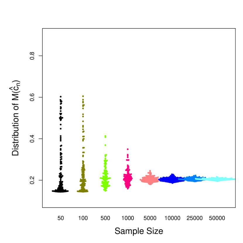
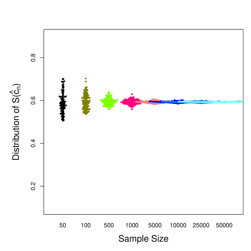
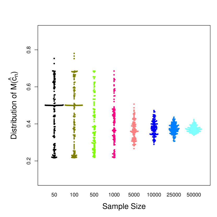
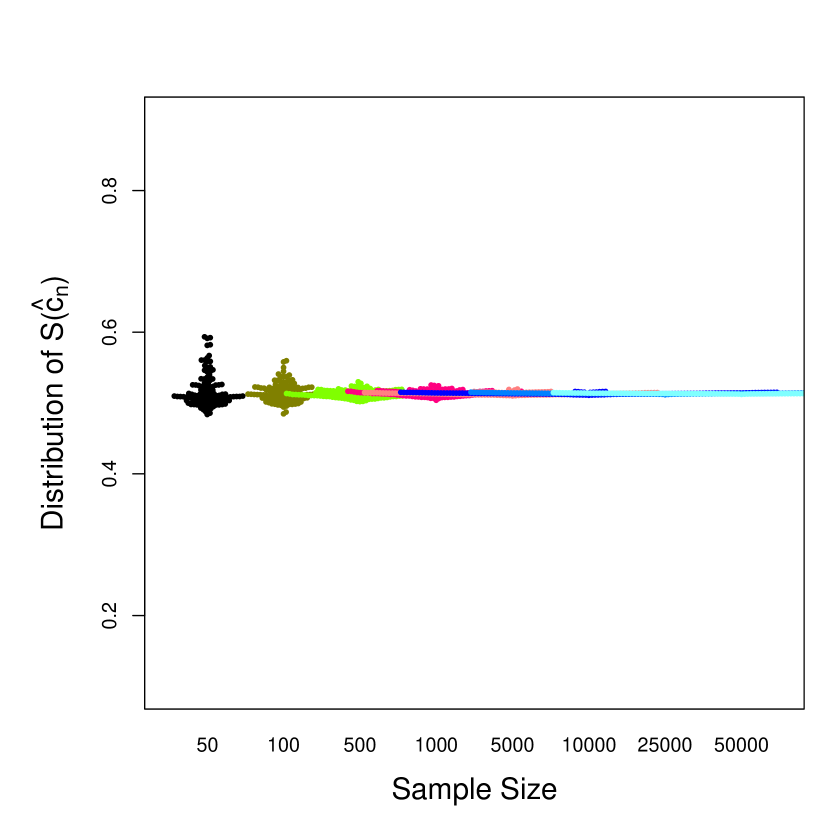
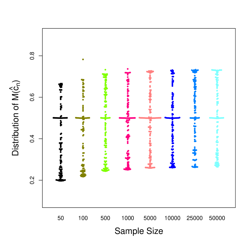
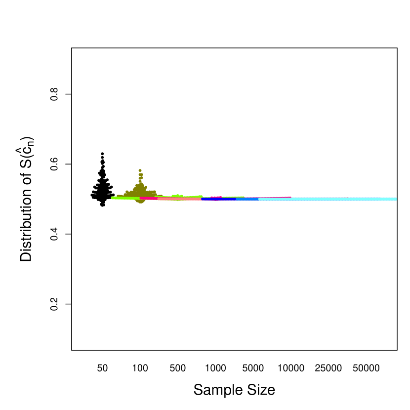
Figure 1: Left column (from top to bottom): 1D histogram of $M(\widehat{c}_{n})$ by training set size for $\delta=0.25$, $\delta=0.10$, and $\delta=1/\sqrt{n})$. Right column (from top to bottom): 1D histogram of $S_{\tau}(\widehat{c}_{n})$ for $\delta=0.25$, $\delta=0.10$, and $\delta=1/\sqrt{n}$.

To highlight the impact of this nonsmoothness, we also draw a sample of size 125 drawn from the distribution of $S_{\tau}(\widehat{c}_{n})\triangleq P\mathrm{expit}\left\{-\tau Y(\widehat{\beta}_{0,n}+\widehat{\beta}_{1,n}X)\right\}$ where $\mathrm{expit}(u)=\exp(u)/\{1+\exp(u)\}$ and $\tau>0$. As $\tau\rightarrow\infty$ the function $\mathrm{expit}(-\tau u)$ converges to $1_{u<0}$; thus, $S(\widehat{c}_{n})$ can be viewed as a smooth surrogate for $M(\widehat{c}_{n})$. In our simulated examples we set $\tau=3$. When $\delta\neq 0$, $M(\widehat{c}_{n})$ converges in probability to $M(c^{\mathrm{opt}})$, where $c^{\mathrm{opt}}({\mbox{\boldmath$x$}})=\mathrm{sign}\left(\beta_{0}^{*}+\beta_{1}^{*}{\mbox{\boldmath$x$}}\right)$. The top left panel of Figure 1 shows a one-dimensional histogram of the distribution of $M(\widehat{c}_{n})$ for $\delta=0.25$ whereas the top right panel of this figure shows one-dimensional histogram for the smooth surrogate $S(\widehat{c}_{n})$ under the same generative model. The higher variability of $M(\widehat{c}_{n})$ relative to $S(\widehat{c}_{n})$ is striking as the $S(\widehat{c}_{n})$ is as tightly clustered about its mean at a training set size of $n=500$ as $M(\widehat{c}_{n})$ is at $n=5000$. This difference can be made more pronounced by choosing a smaller value of $\delta$. The middle left and middle panels of Figure 1 display one-dimensional histograms of $M(\widehat{c}_{n})$ and $S(\widehat{c}_{n})$ for $\delta=0.10$. In this case, $S(\widehat{c}_{n})$ is more tightly clustered about its mean at $n=100$ then $M(\widehat{c}_{n})$ is at $n=50000$. Thus, using the asymptotic limit of $M(\widehat{c}_{n})$ to approximate its finite sample behavior can be arbitrarily poor. Indeed, the lower left and lower right panels of Figure 1 show the one-dimensional histograms of $M(\widehat{c}_{n})$ and $S(\widehat{c}_{n})$ when $\delta=1/\sqrt{n}$; in this case, the variability of $M(\widehat{c}_{n})$ remains the same regardless of how large the sample size grows whereas $S(\widehat{c}_{n})$ quickly concentrates about its mean.

Letting the parameter $\delta$ change with the sample size is an example of a moving-parameter asymptotic analysis. Moving parameter asymptotic analyses are commonly used to study the limiting behavior of nonregular quantities like $M(\widehat{c}_{n})$ as they retain salient small sample behaviors even in infinite samples. In our example, we saw that letting $\delta=O(1/\sqrt{n})$ retained the small-sample instability of $M(\widehat{c}_{n})$ even as $n$ diverged. On the other hand, the concentration of $S(\widehat{c}_{n})$ about its mean was unaffected by letting the parameter $\delta$ vary with $n$. The empirical behavior of $M(\widehat{c}_{n})$ and $S(\widehat{c}_{n})$ is consistent with the formal definition of a nonregular parameter as being sensitive to local (i.e., $O(1/\sqrt{n})$) perturbations of the underlying generative model (Tsiatis, 2007). Because we are interested in asymptotic methods that faithfully reflect the finite sample behavior of the generalization errors we shall consider moving asymptotic arguments in our development of inferential methods.

2.1.1 Confidence intervals for $M(c^{\mathrm{opt}})$

For each $\beta\in\mathbb{R}^{p}$ write $M(\beta)=P\mathbbm{1}\left\{Y{\mbox{\boldmath$X$}}^{\intercal}\beta<0\right\}$ to denote the generalization error for the classification rule $c({\mbox{\boldmath$x$}})=\mathrm{sign}\left({\mbox{\boldmath$x$}}^{\intercal}\beta\right)$; similarly, write $\widehat{M}_{n}(\beta)=\mathbb{P}_{n}\mathbbm{1}\left\{Y{\mbox{\boldmath$X$}}^{\intercal}\beta<0\right\}$ to be the plugin estimator of $M(\beta)$. Define $\sigma^{2}(\beta)=M(\beta)\left\{1-M(\beta)\right\}$ and $\widehat{\sigma}_{n}^{2}(\beta)=\widehat{M}_{n}(\beta)\left\{1-\widehat{M}_{n}(\beta)\right\}$. Were $\beta^{*}$ known, then, as noted previously, $\sqrt{n}\left\{\widehat{M}_{n}(\beta^{*})-M(\beta^{*})\right\}\leadsto\mathrm{Normal}\left\{0,\sigma^{2}(\beta)\right\}$. Thus, for any $\alpha\in(0,1)$ an asymptotic $(1-\alpha)\times 100\%$ confidence interval for $M(\beta^{*})$ is

$$\mathfrak{Z}_{n,1-\alpha}(\beta^{*})=\left[\widehat{M}_{n}(\beta^{*})-\frac{z_{1-\alpha/2}\widehat{\sigma}_{n}(\beta^{*})}{\sqrt{n}},\,\widehat{M}_{n}(\beta^{*})+\frac{z_{1-\alpha/2}\widehat{\sigma}_{n}(\beta^{*})}{\sqrt{n}}\right],$$

where $z_{\nu}$ is the $\nu\times 100$ percentile of a standard normal distribution. Of course $\beta^{*}$ is not generally known and must be estimated using the observed data. However, as we have seen, $\widehat{M}_{n}(\widehat{\beta}_{n})$ need not converge to $M(\beta^{*})$, making $\sqrt{n}\left\{\widehat{M}_{n}(\widehat{\beta}_{n})-M(\beta^{*})\right\}$ a tenuous starting point for inference. Instead, we utilize the fact that $\widehat{\beta}_{n}$ is regular and asymptotically normal to construct a projection confidence interval (Berger and Boos, 1994; Robins, 2004); because projection intervals are notoriously conservative, we also present some refinements intended to reduce conservatism.

Define $\widehat{\Sigma}_{n}\triangleq\left(\mathbb{P}_{n}{\mbox{\boldmath$X$}}{\mbox{\boldmath$X$}}^{\intercal}\right)^{-1}\mathbb{P}_{n}(Y-{\mbox{\boldmath$X$}}^{\intercal}\widehat{\beta}_{n})^{2}{\mbox{\boldmath$X$}}{\mbox{\boldmath$X$}}^{\intercal}\left(\mathbb{P}_{n}{\mbox{\boldmath$X$}}{\mbox{\boldmath$X$}}^{\intercal}\right)^{\intercal}$ to be an estimator of the asymptotic variance-covariance matrix of $\widehat{\beta}_{n}$. For any $\eta\in(0,1)$ a $(1-\eta)\times 100\%$ Wald-type confidence set for $\beta^{*}$ is $\mathfrak{F}_{n,1-\eta}\triangleq\left\{\beta\in\mathbb{R}^{p}\,:\,n\left(\widehat{\beta}_{n}-\beta\right)^{\intercal}\widehat{\Sigma}_{n}^{-1}\left(\widehat{\beta}_{n}-\beta\right)\leq\chi_{n,1-\eta}^{2}\right\}$, where $\chi_{d,\nu}^{2}$ is the $\nu\times 100$ percentile of chi-square random variable with $d$ degrees of freedom. Let $\omega\in(0,1)$ and choose $\eta,\alpha\in(0,1)$ so that $\omega=\alpha+\eta$. A $(1-\omega)\times 100\%$ projection interval for $M(c^{\mathrm{opt}})=M(\beta^{*})$ is $\mathfrak{P}_{n,1-\omega}\triangleq\bigcup_{\beta\in\mathfrak{F}_{n,1-\eta}}\mathfrak{Z}_{n,1-\alpha}(\beta)$. To see that this provides the correct coverage asymptotically write

$$P\left\{M(\beta^{*})\notin\mathfrak{P}_{n,1-\omega}\right\} = P\left\{M(\beta^{*})\notin\mathfrak{P}_{n,1-\omega},\,\beta^{*}\in\mathfrak{F}_{n,1-\eta}\right\}+P\left\{M(\beta^{*})\notin\mathfrak{P}_{n,1-\omega},\,\beta^{*}\notin\mathfrak{F}_{n,1-\eta}\right\}$$

$$\leq P\left\{M(\beta^{*})\notin\mathfrak{Z}_{n,1-\alpha}(\beta*)\right\}+P\left(\beta^{*}\notin\mathfrak{F}_{n,1-\eta}\right)$$

$$\leq \alpha+\eta+o(1)$$

$$= \omega+o(1).$$

Because the projection interval is constructed from continuous operations with regular estimators it is insensitive to local perturbations as we will show below.

To evaluate the local behavior of the generalization error we make the following assumptions.

• The distribution $P$ satisfies $P||Y||^{2}||{\mbox{\boldmath$X$}}||^{2}<\infty$.

• The covariance $\Sigma(\beta)$ is strictly positive definite for all $\beta$ in a neighborhood of $\beta^{*}$.

• For any $\ell\in\mathbb{R}^{p}$ there exists a sequence of distributions $P_{n}$ that satisfies

  $$\int\left[\sqrt{n}\left(dP_{n}^{1/2}-dP^{1/2}\right)-\frac{1}{2}v_{\ell}dP^{1/2}\right]^{2}\rightarrow 0,$$

  for some real-valued function $v_{\ell}$ for which: (i) if $\beta_{n}^{*}=\arg\min_{\beta}P_{n}\left(Y-{\mbox{\boldmath$X$}}^{\intercal}\beta\right)^{2}$ then $\beta_{n}^{*}=\beta^{*}+\ell/\sqrt{n}+o(1/\sqrt{n})$; and (ii) $P_{n}||Y||^{2}||{\mbox{\boldmath$X$}}||^{2}$ is a uniformly bounded sequence.

The following result states that probjection interval remains valid even under a moving parameter asymptotic framework.

Theorem 2.1.

Assume (A1)-(A2) and that for each $n$ the observed data are $\left\{\left({\mbox{\boldmath$X$}}_{i,n},Y_{i,n}\right)\right\}_{i=1}^{n}$ which comprise an $i.i.d.$ draw from $P_{n}$ which satisfies (A3). Let $M_{n}(\beta_{n}^{*})=P_{n}\mathbbm{1}\left\{Y{\mbox{\boldmath$X$}}^{\intercal}\beta_{n}^{*}<0\right\}$, then $P_{n}\left\{M_{n}(\beta_{n}^{*})\in\mathfrak{P}_{n,1-\omega}\right\}\geq 1-\omega+o(1).$

A proof of this result follows from noting that $\sqrt{n}(\widehat{\beta}_{n}-\beta_{n}^{*})\leadsto\mathrm{Normal}\left\{0,\Sigma(\beta^{*})\right\}$ and $\sqrt{n}\left\{\widehat{M}_{n}(\beta)-M_{n}(\beta)\right\}\leadsto\mathrm{Normal}\left\{0,\sigma^{2}(\beta)\right\}$ for each fixed $\beta$ under $P_{n}$; thus, the result follows by applying the argument given for the fixed parameter setting above.

Projection intervals are appealing because of their simplicity and generality. However, they can be extremely conservative in some settings (Laber et al., 2014). One driver for this conservatism is that the projection interval is not adaptive to the concentration of points about the boundary ${\mbox{\boldmath$x$}}^{\intercal}\beta^{*}=0$; e.g., if ${\mbox{\boldmath$X$}}^{\intercal}\beta^{*}$ were bounded away from zero with probability one, then one could just apply the standard nonparametric bootstrap or a normal-based approximation to construct a confidence interval (Efron and Tibshirani, 1994; Shao and Tu, 2012). One can reduce conservatism by adapting the projection interval so that the union only affects points that lie ‘near’ to the decision boundary ${\mbox{\boldmath$x$}}^{\intercal}\beta^{*}$. We formalize the notion of being near the boundary using a hypothesis test of the null $H_{0}({\mbox{\boldmath$x$}}):{\mbox{\boldmath$x$}}^{\intercal}\beta^{*}=0$ against a two-sided alternative for each input ${\mbox{\boldmath$X$}}={\mbox{\boldmath$x$}}$ in the observed data. Define the test statistic $T_{n}({\mbox{\boldmath$x$}})=({\mbox{\boldmath$x$}}^{\intercal}\widehat{\beta}_{n})^{2}/({\mbox{\boldmath$x$}}^{\intercal}\widehat{\Sigma}_{n}{\mbox{\boldmath$x$}})$; we assume (A4) that ${\mbox{\boldmath$X$}}^{\intercal}\widehat{\Sigma}_{n}{\mbox{\boldmath$X$}}$ is bounded away from zero with probability one. We reject $H_{0}({\mbox{\boldmath$x$}})$ if $T_{n}({\mbox{\boldmath$x$}})$ is large and fail to reject otherwise. Let $\lambda_{n}$ denote a positive sequence of critical values (see below for additional restrictions on this sequence) and define

$$\mathbb{G}_{n}(\beta,\beta^{\prime})=P\left[\mathbbm{1}\left\{Y{\mbox{\boldmath$X$}}^{\intercal}\beta<0\right\}\mathbbm{1}\left\{T_{n}({\mbox{\boldmath$X$}})>\lambda_{n}\right\}+\mathbbm{1}\left\{Y{\mbox{\boldmath$X$}}^{\intercal}\beta^{\prime}<0\right\}\mathbbm{1}\left\{T_{n}({\mbox{\boldmath$X$}})\leq\lambda_{n}\right\}\right],$$

then it can be seen that $M(\beta^{*})\triangleq\mathbb{G}_{n}(\beta^{*},\beta^{*})$. Define $\widehat{\mathbb{G}}_{n}(\beta,\beta^{\prime})$ to be the estimator of $\mathbb{G}_{n}$ obtained by replacing $P$ with $\mathbb{P}_{n}$. The following result is the basis for an adaptive projection interval

Lemma 2.2.

Assume (A1)-(A4) and that $\lambda_{n}\to 0$ and $n\lambda_{n}\to\infty$ as $n\to\infty$. For any $\beta\in\mathbb{R}^{p}$ then under either $P$ or $P_{n}$

$$\sqrt{n}\left\{\widehat{\mathbb{G}}_{n}(\widehat{\beta}_{n},\beta)-\mathbb{G}_{n}(\beta^{*},\beta)\right\}\leadsto\mathbb{W}(\beta^{*},\beta),$$

where $\mathbb{W}(\beta^{*},\beta)$ is normally distributed with mean zero and variance $\rho^{2}(\beta^{*},\beta)$.

A proof of this result, which includes a closed form expression for $\rho^{*}(\beta^{*},\beta)$, is given in the Appendix. Let $\widehat{\rho}_{n}^{2}(\beta)$ denote a plugin estimator of $\rho^{2}(\beta^{*},\beta)$ (see the Appendix for details). For any $\alpha\in(0,1)$ define

$$\mathfrak{W}_{n,1-\alpha}(\beta)=\left[\widehat{\mathbb{G}}_{n}(\widehat{\beta}_{n},\beta)-\frac{z_{1-\alpha/2}\widehat{\rho}_{n}(\beta)}{\sqrt{n}},\,\widehat{\mathbb{G}}_{n}(\widehat{\beta}_{n},\beta)+\frac{z_{1-\alpha/2}\widehat{\rho}_{n}(\beta)}{\sqrt{n}}\right],$$

then it follows that $P_{n}\left\{{\mathbb{G}}_{n}(\beta^{*},\beta)\in\mathfrak{W}_{n,1-\alpha}(\beta)\right\}\geq 1-\alpha+o(1)$. For any $\omega,\alpha,\nu\in(0,1)$ such that $\omega=\alpha+\nu$, a $(1-\omega)\times 100\%$ adaptive projection confidence interval for $M(\beta^{*},\beta^{*})$ is $\mathfrak{J}_{n,1-\omega}=\bigcup_{\beta\in\mathfrak{F}_{n,1-\eta}}\mathfrak{W}_{n,1-\alpha}(\beta)$. While the form of the adaptive projection interval $\mathfrak{J}_{n,1-\omega}$ and the standard (non-adaptive) projection interval are similar, the union in $\mathfrak{J}_{n,1-\omega}$ only affects points close to the decision boundary which can make it considerably less conservative in some settings. The following result shows that the adaptive projection interval provides asymptotically correct coverage; a proof is provided in the Appendix.

Theorem 2.3.

Assume (A1), (A2), and (A4). For each $n$ let $\left\{({\mbox{\boldmath$X$}}_{i,n},Y_{i,n})\right\}_{i=1}^{n}$ comprise an $i.i.d.$ draw from $P_{n}$ which satisfies (A3). Let $M_{n}(\beta_{n}^{*})=P_{n}\mathbbm{1}\left\{Y{\mbox{\boldmath$X$}}^{\intercal}\beta_{n}^{*}<0\right\}$ and let $\omega\in(0,1)$ be fixed. Then $P_{n}\left\{M_{n}(\beta_{n}^{*})\in\mathfrak{J}_{n,1-\omega}\right\}\geq 1-\omega+o(1).$

The preceding result was stated in terms of a normal-based confidence interval for $\mathbb{G}_{n}(\beta^{*},\beta)$ for each fixed $\beta$; an alternative, which may provide better finite sample performance, is to use a bootstrap confidence interval instead; extension of the theory to handle this case is straightforward.

2.1.2 Confidence intervals for $M(\widehat{c}_{n})$

To derive a confidence interval for $M(\widehat{\beta}_{n})$ we take a similar approach to the adaptive projection interval in that we partition the training into points that are near the decision boundary ${\mbox{\boldmath$x$}}^{\intercal}\beta^{*}=0$ and points that are far from this boundary. We take a sup over local perturbations of the estimated optimal decision rule to construct an upper bound on the generalization error and an inf to construct a lower bound; we bootstrap these bounds to form a confidence set. Because the supremum (infimum) operation is smooth, the resultant bounds are regular and thereby can be consistently bootstrapped. We derive an upper bound with the derivation of a lower bound being analogous.

Let $T_{n}({\mbox{\boldmath$x$}})$ be as defined in the preceding section and write

$$\sqrt{n}\left\{\widehat{M}_{n}(\widehat{\beta}_{n})-M(\widehat{\beta}_{n})\right\} = \sqrt{n}\left(\mathbb{P}_{n}-P\right)\mathbbm{1}\left\{Y{\mbox{\boldmath$X$}}^{\intercal}\widehat{\beta}_{n}<0\right\}$$

$$= \sqrt{n}(\mathbb{P}_{n}-P)\mathbbm{1}\left\{Y{\mbox{\boldmath$X$}}^{\intercal}\widehat{\beta}_{n}<0\right\}\mathbbm{1}\left\{T_{n}({\mbox{\boldmath$X$}})>\lambda_{n}\right\}$$

$$\quad+\quad\sqrt{n}\left(\mathbb{P}_{n}-P\right)\mathbbm{1}\left\{Y{\mbox{\boldmath$X$}}^{\intercal}\widehat{\beta}_{n}<0\right\}\mathbbm{1}\left\{T_{n}({\mbox{\boldmath$X$}})\leq\lambda_{n}\right\}$$

$$\leq \sqrt{n}(\mathbb{P}_{n}-P)\mathbbm{1}\left\{Y{\mbox{\boldmath$X$}}^{\intercal}\widehat{\beta}_{n}<0\right\}\mathbbm{1}\left\{T_{n}({\mbox{\boldmath$X$}})>\lambda_{n}\right\}$$

$$\quad+\quad\sup_{\beta\in\mathcal{S}_{n}}\sqrt{n}\left(\mathbb{P}_{n}-P\right)\mathbbm{1}\left\{Y{\mbox{\boldmath$X$}}^{\intercal}\beta<0\right\}\mathbbm{1}\left\{T_{n}({\mbox{\boldmath$X$}})\leq\lambda_{n}\right\},$$

$$= \mathcal{U}_{n}(\mathcal{S}_{n})$$

where $\mathcal{S}_{n}$ is any set that contains $\widehat{\beta}_{n}$. We define $\mathcal{U}_{n}=\mathcal{U}_{n}(\mathbb{R}^{p})$ which we use to construct a confidence set; asymptotically, this choice is unimprovable in some sense (Laber and Murphy, 2011) though finite sample performance might be improved by letting $\mathcal{S}_{n}$ depend on the data. Define a lower bound $\mathcal{L}_{n}$ analogously by replacing the $\sup$ with an $\inf$ in the definition of $\mathcal{U}_{n}$.

For any $\alpha\in(0,1)$ let $\widehat{\ell}_{n,\alpha/2}$ denote the $(\alpha/2)\times 100$ percentile of $\mathcal{L}_{n}$ and $\widehat{u}_{n,1-\alpha/2}$ denote the $(1-\alpha/2)\times 100$ percentile of $\mathcal{U}_{n}$ then

$$P\left\{\widehat{M}_{n}(\widehat{\beta}_{n})-\widehat{u}_{n}/\sqrt{n}\leq M(\widehat{\beta}_{n})\leq\widehat{M}_{n}(\widehat{\beta}_{n})-\widehat{\ell}_{n}/\sqrt{n}\right\}\geq 1-\alpha.$$ (1)

Furthermore, if $\widehat{\ell}_{n}(\beta)$ is the $(\alpha/2)\times 100$ percentile of the conditional distribution of $\mathcal{L}_{n}$ given $\widehat{\beta}_{n}=\beta$ and $\widehat{u}_{n}(\beta)$ is the $(1-\alpha/2)\times 100$ percentile of the conditional distribution of $\mathcal{U}_{n}$ given $\widehat{\beta}_{n}=\beta$ then

$$P\left\{\widehat{M}_{n}(\widehat{\beta}_{n})-\widehat{u}_{n}(\widehat{\beta}_{n})/\sqrt{n}\leq M(\widehat{\beta}_{n})\leq\widehat{M}_{n}(\widehat{\beta}_{n})-\widehat{\ell}_{n}(\widehat{\beta}_{n})/\sqrt{n}\Bigg{|}\widehat{\beta}_{n}\right\}\geq 1-\alpha$$ (2)

with probability one. It can be verified directly that both (1) and (2) continue to hold under a sequence of local generative models as in (A3).

In practice, the distributions of the bounds $\mathcal{L}_{n}$ and $\mathcal{U}_{n}$ are not known and thus must be estimated. To estimate the unconditional distribution of these bounds we use the nonparametric bootstrap. Let $\mathbb{P}_{n}^{(b)}$ denote the bootstrap empirical distribution and for a functional $f=f(P,\mathbb{P}_{n})$ write $f^{(b)}=f(\mathbb{P}_{n}\mathbb{P}_{n}^{(b)})$ to denote its bootstrap analog. The following result is proved in Laber and Murphy (2011).

Theorem 2.4.

Assume (A1), (A2), and (A4) and let $\alpha\in(0,1)$ be fixed. Then

$$P\left\{\widehat{M}_{n}(\widehat{\beta}_{n})-\widehat{u}_{n}^{(b)}/\sqrt{n}\leq M(\widehat{\beta}_{n})\leq\widehat{M}_{n}(\widehat{\beta}_{n})-\widehat{\ell}_{n}^{(b)}/\sqrt{n}\right\}\geq 1-\alpha+o_{P}(1).$$

The inequality in the preceding result can be strengthened to equality if ${\mbox{\boldmath$X$}}^{\intercal}\beta^{*}$ is bounded away from zero with probability one.

In order to construct a conditional confidence interval for $M(\widehat{\beta}_{n})$ we first estimate the conditional distribution of the bounds given $\widehat{\beta}_{n}$ and then estimate their conditional quantiles. While it is possible to derive the joint asymptotic distribution of $\left\{\sqrt{n}\left(\widehat{\beta}_{n}-\beta^{*}\right),\mathcal{L}_{n},\mathcal{U}_{n}\right\}$, the form of this limit is complex and hence it is difficult to extract from it the requisite percentiles. Instead, we use a kernel-based bootstrap estimator. Let $K$ denote a multivariate kernel function and $B$ a matrix of bandwidth parameters. Define the estimated conditional CDF of $\mathcal{U}_{n}$ given $\widehat{\beta}_{n}$ as follows

$$\widehat{F}_{\mathcal{U}_{n},n}\left(v\big{|}\beta\right)=\frac{\mathbb{P}_{n}^{(b)}K\left\{B^{-1}(\widehat{\beta}_{n}^{(b)}-\beta)\right\}\mathbbm{1}\left\{\mathcal{U}_{n}^{(b)}\leq v\right\}}{\mathbb{P}_{n}^{(b)}K\left\{B^{-1}(\widehat{\beta}_{n}^{(b)}-\beta)\right\}},$$

subsequently define $\widehat{u}_{n}(\beta)=\widehat{F}_{\mathcal{U}_{n},n}^{-1}(1-\alpha/2;\widehat{\beta}_{n})$ to be the estimated conditional $(1-\alpha/2)\times 100$ percentile of $\mathcal{U}_{n}$ given $\widehat{\beta}_{n}$. Define $\widehat{\ell}_{n}(\widehat{\beta}_{n})$ analogously. An asymptotic $(1-\alpha)\times 100\%$ conditional confidence set for $M(\widehat{\beta}_{n})$ is thus

$$\left[\widehat{M}_{n}(\widehat{\beta}_{n})-\widehat{u}_{n}(\widehat{\beta}_{n})/\sqrt{n},\widehat{M}_{n}(\widehat{\beta}_{n})-\widehat{\ell}_{n}(\widehat{\beta}_{n})/\sqrt{n}\right].$$

A rigorous analysis of the operating characteristics of this interval is beyond the scope of this entry. However, the proof follows by showing: (i) the joint distribution of the bounds and the sampling distribution of $\widehat{\beta}_{n}$ can be consistently estimated using the bootstrap (see Laber and Murphy, 2011); and (ii) that the conditional distribution can be consistently estimated using the preceding kernel-based estimator under an appropriate choice of bandwidth matrix (see Hall et al., 1999, and references therein).

2.1.3 Confidence intervals for $M_{n}(\Gamma)$

Confidence intervals for $M_{n}(\Gamma)$ are less well-studied in the statistics literature primarily because they reflect the average performance across repeated application of the same learning algorithm in the same problem domain; however, it can be argued that methods like cross-validation that estimate the generalization error by repeatedly splitting the data and averaging the performance across splits are really estimating $M_{n}(\Gamma)$ rather than $M(\widehat{c}_{n})$ as is often purported (see Hastie et al., 2009, for a discussion). We derive one potential approach to constructing a confidence set for $M_{n}(\Gamma)$ based on data-adaptive upper and lower bounds as in the preceding section.

Let $\mathbb{F}_{n}$ denote the sampling distribution of $\widehat{\beta}_{n}$, then

$$M_{n}(\Gamma) = \mathbb{E}P\mathbbm{1}\left\{Y{\mbox{\boldmath$X$}}^{\intercal}\widehat{\beta}_{n}<0\right\}$$

$$= \int\mathbbm{1}\left\{y{\mbox{\boldmath$x$}}^{\intercal}\beta<0\right\}dP({\mbox{\boldmath$x$}},y)d\mathbb{F}_{n}(\beta)$$

$$= P\int\mathbbm{1}\left\{Y{\mbox{\boldmath$X$}}^{\intercal}\beta<0\right\}d\mathbb{F}_{n}(\beta),$$

where the last equality follows from interchanging the order of integration. Thus, if $\mathbb{F}_{n}^{(b)}$ is the bootstrap estimator of $\mathbb{F}_{n}$ it can be seen that the plugin estimator of $M_{n}(\Gamma)$ is

$$\widehat{M}_{n}(\Gamma) = \mathbb{E}_{M}\mathbb{P}_{n}\mathbbm{1}\left\{Y{\mbox{\boldmath$X$}}^{\intercal}\widehat{\beta}_{n}^{(b)}<0\right\}$$

$$= \int\mathbbm{1}\left\{y{\mbox{\boldmath$x$}}^{\intercal}\beta<0\right\}d\mathbb{P}_{n}({\mbox{\boldmath$x$}},y)d\mathbb{F}_{n}^{(b)}(\beta)$$

$$= \mathbb{P}_{n}\int\mathbbm{1}\left\{Y{\mbox{\boldmath$X$}}^{\intercal}\beta<0\right\}d\mathbb{F}_{n}^{(b)}(\beta),$$

where $\mathbb{E}_{M}$ denotes expectation with respect to the bootstrap resampling. Let $T_{n}({\mbox{\boldmath$x$}})$ be as defined in the previous section. We will make use of the following bound

$$\sqrt{n}\left\{\widehat{M}_{n}(\Gamma)-M_{n}(\Gamma)\right\} = \sqrt{n}\left[\mathbb{P}_{n}\int\mathbbm{1}\left\{Y{\mbox{\boldmath$X$}}^{\intercal}\beta<0\right\}d\mathbb{F}_{n}^{(b)}(\beta)-P\int\mathbbm{1}\left\{Y{\mbox{\boldmath$X$}}^{\intercal}\beta<0\right\}d\mathbb{F}_{n}(\beta)\right]$$

$$\leq \sqrt{n}\Bigg{[}\mathbb{P}_{n}\mathbbm{1}\left\{T_{n}({\mbox{\boldmath$X$}})>\lambda_{n}\right\}\int\mathbbm{1}\left\{Y{\mbox{\boldmath$X$}}^{\intercal}\beta<0\right\}d\mathbb{F}_{n}^{(b)}(\beta)$$

$$\quad+\quad P\mathbbm{1}\left\{T_{n}({\mbox{\boldmath$X$}})>\lambda_{n}\right\}\int\mathbbm{1}\left\{Y{\mbox{\boldmath$X$}}^{\intercal}\beta<0\right\}d\mathbb{F}_{n}(\beta)\Bigg{]}+\mathbb{S}_{n}$$

$$= \mathfrak{U}_{n},$$

where

$$\mathbb{S}_{n}\triangleq\sup_{\beta\in\mathbb{R}^{p}}\sqrt{n}\Bigg{[}\mathbb{E}_{M}\mathbb{P}_{n}\mathbbm{1}\left\{T_{n}({\mbox{\boldmath$X$}})\leq\lambda_{n}\right\}\mathbbm{1}\left\{Y{\mbox{\boldmath$X$}}^{\intercal}\sqrt{n}\left(\widehat{\beta}_{n}^{(b)}-\beta^{*}\right)+Y{\mbox{\boldmath$X$}}^{\intercal}\beta<0\right\}\\ +\mathbb{E}P\mathbbm{1}\left\{T_{n}({\mbox{\boldmath$X$}})\leq\lambda_{n}\right\}\mathbbm{1}\left\{Y{\mbox{\boldmath$X$}}^{\intercal}\sqrt{n}(\widehat{\beta}_{n}-\beta^{*})+Y{\mbox{\boldmath$X$}}^{\intercal}\beta<0\right\}\Bigg{]}.$$

To verify that $\mathfrak{U}_{n}$ is indeed an upper bound, one can substitute $\sqrt{n}\beta^{*}$ in place of $\beta$. A lower bound, $\mathfrak{L}_{n}$, is obtained by replacing the $\sup$ with an $\inf$. A confidence interval for $M_{n}(\Gamma)$ is obtained using the bootstrap distribution of the bounds $\mathfrak{L}_{n}$ and $\mathfrak{U}_{n}$. Let $\widehat{j}_{n,\alpha/2}$ denote the $(\alpha/2)\times 100$ percentile of $\mathfrak{L}_{n}^{(b)}$ and $\widehat{k}_{n,1-\alpha/2}$ the $(1-\alpha/2)\times 100$ percentile of $\mathfrak{U}_{n}^{(b)}$. The resultant approximate confidence interval for $M_{n}(\Gamma)$ is thus

$$\left[\widehat{M}_{n}(\Gamma)-\frac{\widehat{k}_{n,1-\alpha/2}}{\sqrt{n}},\,\widehat{M}_{n}(\Gamma)-\frac{\widehat{j}_{n,\alpha/2}}{\sqrt{n}}\right].$$

The operating characteristics of the above interval have not yet been fully investigated; such an investigation is beyond the scope of this entry, though we think this would make for interesting future work.

3 Marginal mean outcome in decision making

In a one-stage decision problem we assume that the observed data are of the form $\left\{({\mbox{\boldmath$X$}}_{i},A_{i},Y_{i})\right\}_{i=1}^{n}$ which comprise $n$ independent replicates of the triple $({\mbox{\boldmath$X$}},A,Y)$, where: ${\mbox{\boldmath$X$}}\in\mathbb{R}^{p}$ describes the decision context; $A\in\left\{-1,1\right\}$ is the decision; and $Y\in\mathbb{R}$ is the outcome coded so that higher values are better. A common application is precision medicine wherein: $X$ denotes baseline patient characteristics, $A$ is their assigned treatment, and $Y$ is the patient’s clinical outcome (Qian and Murphy, 2011; Zhao et al., 2012; Zhang et al., 2012; Chakraborty and Moodie, 2013; Kosorok and Moodie, 2015). A decision rule, $d:\mathrm{dom}\,{\mbox{\boldmath$X$}}\rightarrow\mathrm{dom}\,A$, so that a decision maker following $d$ would make decision $d({\mbox{\boldmath$x$}})$ in the context ${\mbox{\boldmath$X$}}={\mbox{\boldmath$x$}}$. An optimal decision rules, $d^{\mathrm{opt}}$, maximized the mean outcome if applied over the distribution of contexts. The one-stage decision problem is closely related to the classification problem studied previously. The critical difference lies in the information contained in the available data. In a decision problem as described above, the outcome $Y$ provides indirect feedback about the quality of decision $A$ in context $X$; in contrast, in a classification problem, one would be given the context $X$ and the optimal decision $d^{\mathrm{opt}}({\mbox{\boldmath$X$}})$ (see Sutton and Barto, 1998).

We formalize an optimal regime using the language of potential outcomes Rubin (1978); Splawa-Neyman et al. (1990). Let $Y^{*}(a)$ denote the potential outcome under decision $a\in\mathrm{dom}\,A$. Then the potential outcome under a decision rule $d$ is $Y^{*}(d)=\sum_{a}Y^{*}(a)\mathbbm{1}\left\{d({\mbox{\boldmath$X$}})=a\right\}$. Given a class of decision rules, $\mathcal{D}$, we define an optimal decision rule, $d^{\mathrm{opt}}\in\mathcal{D}$, as one that satisfies $PY^{*}(d^{\mathrm{opt}})\geq PY^{*}(d)$ for all $d\in\mathcal{D}$. In order to identify $d^{\mathrm{opt}}$ in terms of the data-generating model, we make the following assumptions: (C1) positivity, $\pi(a;{\mbox{\boldmath$x$}})\triangleq P(A=a|{\mbox{\boldmath$X$}}={\mbox{\boldmath$x$}})>0$ with probability one for each $a\in\mathrm{dom}\,A$ and ${\mbox{\boldmath$x$}}\in\mathrm{dom}\,{\mbox{\boldmath$X$}}$; (C2) no unmeasured confounding, $\left\{Y^{*}(a)\,:\,a\in\mathrm{dom}\,A\right\}\perp A\big{|}{\mbox{\boldmath$X$}}$; and (C3) consistency, $Y=Y^{*}(A)$. These assumptions are standard in single stage decision problems (Zhang et al., 2012); (C1) and (C2) can be guaranteed in a randomized experiment but (C2) is not verifiable in an observational studies.

Under (C1)-(C3) it follows that the marginal mean outcome under a given decision rule $d$ can be expressed as

$$V(d)=P\left[\frac{Y\mathbbm{1}\left\{d({\mbox{\boldmath$X$}})=A\right\}}{P\left(A\big{|}{\mbox{\boldmath$X$}}\right)}\right]=P\left[\frac{Y\mathbbm{1}\left\{d({\mbox{\boldmath$X$}})\neq-A\right\}}{P\left(A\big{|}{\mbox{\boldmath$X$}}\right)}\right],$$ (3)

which can be viewed as a weighted misclassification rate for $d$ with labels $-A$ and weights $Y/P(A|{\mbox{\boldmath$X$}})$; however, in this formulation it should be emphasized that all the unobserved actions $-A$ need not be the correct labels, i.e., the need need not equal $d^{\mathrm{opt}}({\mbox{\boldmath$X$}})$, indeed if there observed data were generated in a randomized clinical trial $A$ would be assigned at random (see Zhang et al., 2012; Zhang et al., 2013; Zhang and Zhang, 2015, for additional discussion). Nevertheless, the expression for $V(d)$ in (3) can be used to directly extend the inferential methods for the generalization error in classification to the marginal mean outcome in the single-stage decision setting.

As in the classification setting, for the purpose of illustration, we consider linear models fit using least squares; extensions to other smooth parametric models and convex loss functions is straightforward. Define $Q({\mbox{\boldmath$x$}},a)=\mathbb{E}(Y|{\mbox{\boldmath$X$}}={\mbox{\boldmath$x$}},A=a)$ then, under (C1)-(C3), $d^{\mathrm{opt}}({\mbox{\boldmath$x$}})=\arg\max_{a}Q({\mbox{\boldmath$x$}},a)$ (Murphy, 2005; Qian and Murphy, 2011; Schulte et al., 2014; Kosorok and Moodie, 2015). Thus, a natural approach to estimating $d^{\mathrm{opt}}$ based on the preceding characterization is to construct an estimator $\widehat{Q}_{n}({\mbox{\boldmath$x$}},a)$ of $Q({\mbox{\boldmath$x$}},a)$ and then to use the plugin estimator $\widehat{d}_{n}({\mbox{\boldmath$x$}})=\arg\max_{a}\widehat{Q}_{n}({\mbox{\boldmath$x$}},a)$. We take this approach using linear working models of the form $Q({\mbox{\boldmath$x$}},a;\beta)={\mbox{\boldmath$x$}}_{0}^{\intercal}\beta_{0}+a{\mbox{\boldmath$x$}}_{1}^{\intercal}\beta_{1}$, where $\beta=(\beta_{0}^{\intercal},\beta_{1}^{\intercal})^{\intercal}$ and ${\mbox{\boldmath$x$}}_{0},{\mbox{\boldmath$x$}}_{1}$ are features constructed from $x$. Define $\widehat{\beta}_{n}=\arg\min_{\beta}\mathbb{P}_{n}\left\{Y-Q({\mbox{\boldmath$X$}},A;\beta)\right\}^{2}$ and subsequently $\widehat{d}_{n}({\mbox{\boldmath$x$}})=\arg\max_{a}Q({\mbox{\boldmath$x$}},a;\widehat{\beta}_{n})$. Define the population analog of $\widehat{\beta}_{n}$ to be $\beta^{*}=\arg\min_{\beta}P\left\{Y-Q({\mbox{\boldmath$X$}},A;\beta)\right\}^{2}$ and subsequently $d^{\mathrm{opt}}({\mbox{\boldmath$x$}})=\arg\max_{a}Q({\mbox{\boldmath$x$}},a;\beta^{*})$.

Given $\beta$, write $V(\beta)$ to denote the expected outcome under the rule $d({\mbox{\boldmath$x$}})=\arg\max_{a}Q({\mbox{\boldmath$x$}},a;\beta)=\mathrm{sign}\left({\mbox{\boldmath$x$}}_{1}^{\intercal}\beta_{1}\right)$. Thus, $V(\beta^{*})$ denotes the marginal mean outcome associated with the decision rule $d^{\mathrm{opt}}$; thus, $V(\beta^{*})$ is analogous to $M(\beta^{*})$ and one can use a projection interval to construct an asymptotically valid confidence set. Suppose first that the propensity score, $\pi(a;{\mbox{\boldmath$x$}})$ is known, and for fixed $\beta$ define $\widehat{V}_{n}(\beta)=\mathbb{P}_{n}\left[Y\mathbbm{1}\left\{-A{\mbox{\boldmath$X$}}_{1}^{\intercal}\beta_{1}<0\right\}/\pi(A;{\mbox{\boldmath$X$}})\right]$. For any fixed $\beta$ it follows from the central limit theorem that $\sqrt{n}\left\{\widehat{V}_{n}(\beta)-V(\beta)\right\}$ is asymptotically normal with mean zero and variance

$$\varsigma^{*2}(\beta)=P\left[\frac{Y\mathbbm{1}\left\{-A{\mbox{\boldmath$X$}}_{1}^{\intercal}\beta_{1}<0\right\}}{\pi({\mbox{\boldmath$X$}};A)}-P\left\{\frac{Y\mathbbm{1}\left\{-A{\mbox{\boldmath$X$}}_{1}^{\intercal}\beta_{1}<0\right\}}{\pi({\mbox{\boldmath$X$}};A)}\right\}\right]^{2}.$$

Let $\widehat{\varsigma}_{n}^{2}(\beta)$ denote the plug-in estimator of $\varsigma^{*2}(\beta)$ obtained by replacing $P$ with $\mathbb{P}_{n}$ in the foregoing expression. For any $\alpha\in(0,1)$, define

$$\mathfrak{V}_{n,1-\alpha}(\beta)\triangleq\left[\widehat{V}_{n}(\beta)-\frac{z_{1-\alpha/2}\widehat{\varsigma}_{n}(\beta)}{\sqrt{n}},\,\widehat{V}_{n}(\beta)+\frac{z_{1-\alpha/2}\widehat{\varsigma}_{n}(\beta)}{\sqrt{n}}\right],$$

which is an asymptotic $(1-\alpha)\times 100\%$ confidence interval for $V(\beta)$. Given $\eta\in(0,1)$ let $\mathfrak{Q}_{n,1-\eta}$ be a $(1-\eta)\times 100\%$ confidence set for $\beta^{*}$ (e.g., one could construct a Wald-type confidence set as in the preceding section). For any $\omega\in(0,1)$ choose $\eta,\alpha\in(0,1)$ so that $\omega=\alpha+\eta$, then a $(1-\omega)\times 100\%$ confidence set for $V(\beta^{*})$ is $\bigcup_{\beta\in\mathfrak{Q}_{n,1-\eta}}\mathfrak{V}_{n,1-\alpha}(\beta)$. The theoretical properties of the projection interval for $M(\beta^{*})$ developed in the preceding section port directly to the confidence interval for $V(\beta^{*})$; moreover, one can also construct an adaptive projection interval to reduce conservatism. The extension to the case where the propensity score is unknown is straightforward provided that one estimates the propensity score using a regular asymptotically linear estimator.

The marginal mean outcome for the estimated optimal decision rule $\widehat{d}_{n}$ is $V(\widehat{\beta}_{n})=P\left[Y\mathbbm{1}\left\{-A{\mbox{\boldmath$X$}}_{1}^{\intercal}\widehat{\beta}_{1,n}<0\right\}/\pi(A;{\mbox{\boldmath$X$}})\right]$ which is analogous to $M_{n}(\widehat{\beta}_{n})$ in the classification case. Define $\widehat{V}_{n}=\mathbb{P}_{n}\left[Y\mathbbm{1}\left\{-A{\mbox{\boldmath$X$}}_{1}^{\intercal}\widehat{\beta}_{1,n}<0\right\}/\pi(A;{\mbox{\boldmath$X$}})\right]$, mimicking the classification setting, we construct confidence bounds for $V(\widehat{\beta}_{n})$ using smooth upper and lower bounds on $\sqrt{n}\left\{\widehat{V}_{n}-V(\widehat{\beta}_{n})\right\}$; the derivation of these bounds is essentially identical to those used in the classification setting. Let $\widehat{R}_{n}$ denote the plug-in estimator of the asymtptotic covariance of $\widehat{\beta}_{1,n}$ and define $Z_{n}({\mbox{\boldmath$X$}})=n({\mbox{\boldmath$X$}}_{1}^{\intercal}\widehat{\beta}_{1,n})^{2}/{\mbox{\boldmath$X$}}_{1}^{\intercal}\widehat{R}_{n}{\mbox{\boldmath$X$}}_{1}$. For any sequence of non-negative tuning parameters $\left\{\varrho_{n}\right\}_{n\geq 1}$ the following inequality holds

$$\sqrt{n}\left\{\widehat{V}_{n}-V(\widehat{\beta}_{n})\right\}\leq\sqrt{n}\left(\mathbb{P}_{n}-P\right)\left[\frac{Y\mathbbm{1}\left\{-A{\mbox{\boldmath$X$}}_{1}^{\intercal}\widehat{\beta}_{1,n}<0\right\}\mathbbm{1}\left\{Z_{n}({\mbox{\boldmath$X$}})>\varrho_{n}\right\}}{\pi(A;{\mbox{\boldmath$X$}})}\right]\\ +\sup_{\beta\in\mathcal{J}_{n}}\sqrt{n}\left(\mathbb{P}_{n}-P\right)\left[\frac{Y\mathbbm{1}\left\{-A{\mbox{\boldmath$X$}}_{1}^{\intercal}\beta<0\right\}\mathbbm{1}\left\{Z_{n}({\mbox{\boldmath$X$}})\leq\varrho_{n}\right\}}{\pi(A;{\mbox{\boldmath$X$}})}\right],$$

provided that $\widehat{\beta}_{1,n}\in\mathcal{J}_{n}$. Let $\mathcal{E}_{n}$ denote the upper bound obtained by setting $\mathcal{J}_{n}=\mathbb{R}^{{\text{dim}}\,{\mbox{\boldmath$X$}}_{1}}$ and let $\mathcal{M}_{n}$ denote an analogous lower bound obtained by replacing the $\sup$ with an $\inf$ in the definition of $\mathcal{E}_{n}$. A confidence interval for $V(\widehat{\beta}_{n})$ is obtained by taking the percentiles of the bootstrap distribution of these upper and lower bounds; theoretical properties can be derived from analogous arguments to those used in for bound-based inference for $M(\widehat{\beta}_{n})$. Similarly, one can derive bounds for $\mathbb{E}V(\widehat{\beta}_{n})$ my mimicking those for $M_{n}(\Gamma)$; thus, we omit such derivations.

4 Discussion

We provided a whirlwind tour of confidence intervals for the generalization error in classification and the marginal mean outcome in single-stage decision problems. We delineated three types of generalization error and argued that: (i) these need not be close even asymptotically; and (ii) even when they converge to the same limit this convergence is not uniform and consequently they need not be close in finite samples. The implication is that inference procedures for the generalization error (or the marginal mean outcome in decision problems) must be consistent under moving parameter asymptotics if they are to be relied upon in practice.

There are a number of interesting extensions and alternative approaches that we did not cover in this entry. Perhaps the biggest omission was a lack of discussion of subsampling-based approaches. The m-out-of-n bootstrap and substampling without replacement are a common approach to inference in nonregular problems like those considered here (Chakraborty et al., 2014, 2013). However, such procedures can be difficult to tune and in some cases perform worse than naive bootstrap or normal approximations (Samworth, 2003). The inference procedures we reviewed (and the few new ones we introduced) were based on asymptotic arguments. However, in some settings, finite sample (i.e., non-asymptotic) bounds may be desired. There is a large body of literature on such bounds in statistics and computer science (see Murphy, 2005; Qian and Murphy, 2011, and references therein). These bounds can provide a more refined characterization of the relationship between the instability of the generalization error in finite samples and the amassing of points near the optimal decision boundary. In the context of decision problems an important extension is to multi-stage settings; the primary complication in this extension is that the estimators indexing the underlying models are nonregular so that bound-based and projection-based intervals become considerably more involved (Laber et al., 2014).

5 Acknowledgments

This work was partially supported by NSF grantsDMS-1555141 and DMS-1513579 and NIH grants R01-DK-108073, 1R01 AA023187-01A1, P01 CA142538, and R21-MH-108999.

6 Related articles

Davidian, Marie, Anastasios A. Tsiatis, and Eric B. Laber. ”Optimal Dynamic Treatment Regimes.” Wiley StatsRef: Statistics Reference Online (2016).

7 Appendix: additional technical details

7.1 Proof of Lemma 2.2

We can rewrite $\sqrt{n}(\widehat{\mathbb{G}}_{n}(\widehat{\beta}_{n},\beta)-\mathbb{G}_{n}(\beta_{n}^{*},\beta))$ as

$$\sqrt{n}(\widehat{\mathbb{G}}_{n}(\widehat{\beta}_{n},\beta)-\mathbb{G}_{n}(\beta_{n}^{*},\beta))$$ (4)

$$= P_{n}\left[\sqrt{n}\left(\mathbbm{1}\left\{Y{\mbox{\boldmath$X$}}^{\intercal}\widehat{\beta}_{n}<0\right\}-\mathbbm{1}\left\{Y{\mbox{\boldmath$X$}}^{\intercal}\beta_{n}^{*}<0\right\}\right)\mathbbm{1}\left\{T_{n}({\mbox{\boldmath$X$}})>\lambda_{n}\right\}\right]$$

$$+\sqrt{n}(\mathbb{P}_{n}-P_{n})\left[\left(\mathbbm{1}\left\{Y{\mbox{\boldmath$X$}}^{\intercal}\widehat{\beta}_{n}<0\right\}-\mathbbm{1}\left\{Y{\mbox{\boldmath$X$}}^{\intercal}\beta_{n}^{*}<0\right\}\right)\mathbbm{1}\left\{T_{n}({\mbox{\boldmath$X$}})>\lambda_{n}\right\}\right]$$

$$+\sqrt{n}(\mathbb{P}_{n}-P_{n})\left[\mathbbm{1}\left\{Y{\mbox{\boldmath$X$}}^{\intercal}\beta_{n}^{*}<0\right\}\mathbbm{1}\left\{T_{n}({\mbox{\boldmath$X$}})>\lambda_{n}\right\}+\mathbbm{1}\left\{Y{\mbox{\boldmath$X$}}^{\intercal}\beta<0\right\}\mathbbm{1}\left\{T_{n}({\mbox{\boldmath$X$}})\leq\lambda_{n}\right\}\right]$$

Under Assumptions (A1)-(A3), $\sqrt{n}(\widehat{\beta}_{n}-\beta_{n}^{*})\stackrel{{\scriptstyle d}}{{\to}}N(0,\Sigma(\beta^{*}))$ and $\sqrt{n}(\beta^{*}_{n}-\beta^{*})=O(1)$. Thus for every ${\mbox{\boldmath$x$}}\in\mathbb{R}^{p}$,

$$nT_{n}({\mbox{\boldmath$x$}})=n[{\mbox{\boldmath$x$}}^{\intercal}(\widehat{\beta}_{n}-\beta_{n}^{*})+{\mbox{\boldmath$x$}}^{\intercal}({\beta}^{*}_{n}-\beta^{*})+{\mbox{\boldmath$x$}}^{\intercal}\beta^{*}]^{2}/({\mbox{\boldmath$x$}}^{\intercal}\widehat{\Sigma}_{n}{\mbox{\boldmath$x$}})=[{\mbox{\boldmath$x$}}^{\intercal}(\sqrt{n}\beta^{*}+O_{P}(1))]^{2}/({\mbox{\boldmath$x$}}^{\intercal}\widehat{\Sigma}_{n}{\mbox{\boldmath$x$}}).$$

By Continuous Mapping Theorem, under Assumption (A4) and the condition that $\lambda_{n}\to 0$ and $n\lambda_{n}\to\infty$, $\mathbbm{1}\left\{T_{n}({\mbox{\boldmath$x$}})>\lambda_{n}\right\}\to\mathbbm{1}\left\{{\mbox{\boldmath$x$}}^{\intercal}\beta^{*}\neq 0\right\}$ in probability pointwise. Similarly, we can show that $\sqrt{n}\left(\mathbbm{1}\left\{y{\mbox{\boldmath$x$}}^{\intercal}\widehat{\beta}_{n}<0\right\}-\mathbbm{1}\left\{y{\mbox{\boldmath$x$}}^{\intercal}\beta_{n}^{*}<0\right\}\right)\mathbbm{1}\left\{T_{n}({\mbox{\boldmath$x$}})>\lambda_{n}\right\}$ converges pointwise to zero in probability. Using Dominated Convergence Theorem, we have

$$P\left[|\mathbbm{1}\left\{T_{n}({\mbox{\boldmath$X$}})>\lambda_{n}\right\}-\mathbbm{1}\left\{{\mbox{\boldmath$X$}}^{\intercal}\beta^{*}\neq 0\right|\right]\to 0$$

in probability, and the first term of (4) converges to zero in probability. Using similar arguments as those in the proof of Lemma 19.24 of Van der Vaart (1998), the second term of (4) converges to zero in probability, and the third term converges to a normal distribution with mean zero and variance

$$\rho^{2}(\beta^{*},\beta)={\rm Var}\left(\mathbbm{1}\left\{Y{\mbox{\boldmath$X$}}^{\intercal}\beta^{*}<0\right\}\mathbbm{1}\left\{{\mbox{\boldmath$X$}}^{\intercal}\beta^{*}\neq 0\right\}+\mathbbm{1}\left\{Y{\mbox{\boldmath$X$}}^{\intercal}\beta<0\right\}\mathbbm{1}\left\{{\mbox{\boldmath$X$}}^{\intercal}\beta^{*}=0\right\}\right).$$

This completes the proof.

7.2 Proof of Theorem 2.3

Note that

$$P_{n}\left\{M_{n}(\beta_{n}^{*})\notin\mathfrak{J}_{n,1-\omega}\right\} = P_{n}\left\{M_{n}(\beta_{n}^{*})\notin\mathfrak{J}_{n,1-\omega},\,\beta_{n}^{*}\in\mathfrak{F}_{n,1-\eta}\right\}+P_{n}\left\{M_{n}(\beta_{n}^{*})\notin\mathfrak{J}_{n,1-\omega},\,\beta_{n}^{*}\notin\mathfrak{F}_{n,1-\eta}\right\}$$

$$\leq P_{n}\left\{M_{n}(\beta_{n}^{*})\notin\mathfrak{W}_{n,1-\alpha}(\beta_{n}^{*})\right\}+P_{n}\left(\beta_{n}^{*}\notin\mathfrak{F}_{n,1-\eta}\right)$$

$$\leq \alpha+\eta+o(1)$$

where the last inequality follows from Lemma 2.2, the fact that $M_{n}(\beta_{n}^{*})=\mathbb{G}_{n}(\beta^{*}_{n},\beta^{*}_{n})$, and $\sqrt{n}(\widehat{\beta}_{n}-\beta_{n}^{*})\stackrel{{\scriptstyle d}}{{\to}}N(0,\Sigma(\beta^{*}))$. The result follows immediately.

References

• Amari et al. (1992) Amari, S.-i., N. Fujita, and S. Shinomoto (1992). Four types of learning curves. Neural Computation 4(4), 605–618.
• Bartlett et al. (2006) Bartlett, P. L., M. I. Jordan, and J. D. McAuliffe (2006). Convexity, classification, and risk bounds. Journal of the American Statistical Association 101(473), 138–156.
• Berger and Boos (1994) Berger, R. L. and D. D. Boos (1994). P values maximized over a confidence set for the nuisance parameter. Journal of the American Statistical Association 89(427), 1012–1016.
• Casella (1992) Casella, G. (1992). Conditional inference from confidence sets. Lecture Notes-Monograph Series, 1–12.
• Chakraborty et al. (2013) Chakraborty, B., E. B. Laber, and Y. Zhao (2013). Inference for optimal dynamic treatment regimes using an adaptive m-out-of-n bootstrap scheme. Biometrics 69(3), 714–723.
• Chakraborty et al. (2014) Chakraborty, B., E. B. Laber, and Y.-Q. Zhao (2014). Inference about the expected performance of a data-driven dynamic treatment regime. Clinical Trials 11(4), 408–417.
• Chakraborty and Moodie (2013) Chakraborty, B. and E. E. Moodie (2013). Statistical Methods for Dynamic Treatment Regimes. Springer.
• Dawid (1994) Dawid, A. (1994). Selection paradoxes of bayesian inference. Lecture Notes-Monograph Series, 211–220.
• Duda et al. (2012) Duda, R. O., P. E. Hart, and D. G. Stork (2012). Pattern classification. John Wiley & Sons.
• Efron and Tibshirani (1997) Efron, B. and R. Tibshirani (1997). Improvements on cross-validation: the 632+ bootstrap method. Journal of the American Statistical Association 92(438), 548–560.
• Efron and Tibshirani (1994) Efron, B. and R. J. Tibshirani (1994). An introduction to the bootstrap, Volume 57. CRC press.
• Hall et al. (1999) Hall, P., R. C. Wolff, and Q. Yao (1999). Methods for estimating a conditional distribution function. Journal of the American Statistical association 94(445), 154–163.
• Hastie et al. (2009) Hastie, T., R. Tibshirani, J. Friedman, T. Hastie, J. Friedman, and R. Tibshirani (2009). The elements of statistical learning, Volume 2. Springer.
• Haussler et al. (1996) Haussler, D., M. Kearns, H. S. Seung, and N. Tishby (1996). Rigorous learning curve bounds from statistical mechanics. Machine Learning 25(2-3), 195–236.
• Hirano and Porter (2012) Hirano, K. and J. R. Porter (2012). Impossibility results for nondifferentiable functionals. Econometrica 80(4), 1769–1790.
• Kosorok and Moodie (2015) Kosorok, M. R. and E. E. Moodie (2015). Adaptive treatment strategies in practice: planning trials and analyzing data for personalized medicine. SIAM.
• Laber et al. (2014) Laber, E. B., D. J. Lizotte, M. Qian, W. E. Pelham, and S. A. Murphy (2014). Dynamic treatment regimes: Technical challenges and applications. Electronic journal of statistics 8(1), 1225.
• Laber and Murphy (2011) Laber, E. B. and S. A. Murphy (2011). Adaptive confidence intervals for the test error in classification. Journal of the American Statistical Association 106(495), 904–913.
• Laber et al. (2016) Laber, E. B., K. Shedden, and Y. Yang (2016). An imputation method for estimating the learning curve in classification problems. In Statistical Analysis for High-Dimensional Data, pp. 189–209. Springer.
• Laber et al. (2016) Laber, E. B., Y.-Q. Zhao, T. Regh, M. Davidian, A. Tsiatis, J. B. Stanford, D. Zeng, R. Song, and M. R. Kosorok (2016). Using pilot data to size a two-arm randomized trial to find a nearly optimal personalized treatment strategy. Statistics in medicine 35(8), 1245–1256.
• Luckett et al. (2018) Luckett, D., E. Laber, S. El-Kamary, C. Fan, R. Jhaveri, C. Perou, F. Shebl, and M. Kosorok (2018). Receiver operating characteristic curves and confidence bands for support vector machines. Under review.
• Mukherjee et al. (2003) Mukherjee, S., P. Tamayo, S. Rogers, R. Rifkin, A. Engle, C. Campbell, T. R. Golub, and J. P. Mesirov (2003). Estimating dataset size requirements for classifying dna microarray data. Journal of computational biology 10(2), 119–142.
• Murphy (2005) Murphy, S. A. (2005, Jul). A generalization error for Q-learning. Journal of Machine Learning Research 6, 1073–1097.
• Qian and Murphy (2011) Qian, M. and S. Murphy (2011). Performance Guarantees for Individualized Treatment Rules. The Annals of Statistics 39(2), 1180–1210.
• Robins et al. (2014) Robins, J., A. Rotnitzky, et al. (2014). Discussion of “dynamic treatment regimes: Technical challenges and applications”. Electronic Journal of Statistics 8(1), 1273–1289.
• Robins (2004) Robins, J. M. (2004). Optimal structural nested models for optimal sequential decisions. In Proceedings of the Second Seattle Symposium on Biostatitics, pp.  189–326. Springer.
• Rubin (1978) Rubin, D. (1978). Bayesian inference for causal effects: The role of randomization. The Annals of Statistics 6(1), 34–58.
• Samworth (2003) Samworth, R. (2003). A note on methods of restoring consistency to the bootstrap. Biometrika 90(4), 985–990.
• Schiavo and Hand (2000) Schiavo, R. A. and D. J. Hand (2000). Ten more years of error rate research. International Statistical Review 68(3), 295–310.
• Schulte et al. (2014) Schulte, P., A. Tsiatis, E. Laber, , and M. Davidian (2014). Q- and a-learning methods for estimating optimal dynamic treatment regimes. Statistical Science 29(4), 640–661.
• Seber and Lee (2012) Seber, G. A. and A. J. Lee (2012). Linear regression analysis, Volume 936. John Wiley & Sons.
• Shao and Tu (2012) Shao, J. and D. Tu (2012). The jackknife and bootstrap. Springer Science & Business Media.
• Splawa-Neyman et al. (1990) Splawa-Neyman, J., D. Dabrowska, T. Speed, et al. (1990). On the application of probability theory to agricultural experiments. essay on principles. section 9. Statistical Science 5(4), 465–472.
• Stefanski and Boos (2002) Stefanski, L. A. and D. D. Boos (2002). The calculus of m-estimation. The American Statistician 56(1), 29–38.
• Sutton and Barto (1998) Sutton, R. and A. Barto (1998). Reinforcment Learning: An Introduction. The MIT Press.
• Tsiatis (2007) Tsiatis, A. (2007). Semiparametric theory and missing data. Springer Science & Business Media.
• Van der Vaart (1991) Van der Vaart, A. (1991). On differentiable functionals. The Annals of Statistics, 178–204.
• Van der Vaart (1998) Van der Vaart, A. W. (1998). Asymptotic statistics, Volume 2. Cambridge university press.
• Zhang et al. (2012) Zhang, B., A. A. Tsiatis, M. Davidian, M. Zhang, and E. Laber (2012). Estimating optimal treatment regimes from a classification perspective. Stat 1(1), 103–114.
• Zhang et al. (2012) Zhang, B., A. A. Tsiatis, E. B. Laber, and M. Davidian (2012). A robust method for estimating optimal treatment regimes. Biometrics 68(4), 1010–1018.
• Zhang et al. (2013) Zhang, B., A. A. Tsiatis, E. B. Laber, and M. Davidian (2013). Robust estimation of optimal dynamic treatment regimes for sequential treatment decisions. Biometrika 100(3), 681–694.
• Zhang and Zhang (2015) Zhang, B. and M. Zhang (2015). C-learning: A new classification framework to estimate optimal dynamic treatment regimes. Biometrics.
• Zhang (1995) Zhang, P. (1995). Ape and models for categorical panel data. Scandinavian Journal of Statistics 22, 83–94.
• Zhao et al. (2012) Zhao, Y., D. Zeng, A. J. Rush, and M. R. Kosorok (2012). Estimating individualized treatment rules using outcome weighted learning. Journal of the American Statistical Association 107(499), 1106–1118.