Type I Abelian Higgs strings: evolution and Cosmic Microwave Background constraints

Abstract

We present results from the first simulations of networks of Type I Abelian Higgs cosmic strings to include both matter and radiation eras and Cosmic Microwave Background (CMB) constraints. In Type I strings, the string tension is a slowly decreasing function of the ratio of the scalar and gauge mass-squared, $\beta$. We find that the mean string separation shows no dependence on $\beta$, and that the energy-momentum tensor correlators decrease approximately in proportion to the square of the string tension, with additional O(1) correction factors which asymptote to constants below $\beta\lesssim 0.01$. Strings in models with low self-couplings can therefore satisfy current CMB bounds at higher symmetry-breaking scales. This is particularly relevant for models where the gauge symmetry is broken in a supersymmetric flat direction, for which the effective self-coupling can be extremely small. If our results can be extrapolated to $\beta\simeq 10^{-15}$, even strings formed at $10^{16}$ GeV (approximately the grand unification scale in supersymmetric extensions of the Standard Model) can be compatible with CMB constraints.

I Introduction

Topological defects are a common by-product of phase transitions in the early Universe Kibble (1976). Many kinds of defect are possible Vilenkin and Shellard (1994), but perhaps the most well-motivated for study in cosmology are cosmic strings: they are expected for many realistic multi-field models of inflation Jeannerot et al. (2003), and they remain a constant small fraction of the energy density throughout the history of the Universe Zeldovich (1980); Vilenkin (1981a), neither dominating nor disappearing. More about the cosmic string scenario can be found in review articles Hindmarsh and Kibble (1995); Sakellariadou (2007); Copeland et al. (2011); Hindmarsh (2011).

If cosmic strings are formed then they will create characteristic observational signals from their metric perturbations and their decay products. The most significant are Cosmic Microwave Background (CMB) fluctuations Gott (1985); Kaiser and Stebbins (1984), gravitational waves Vilenkin (1981b); Hogan and Rees (1984), and high-energy cosmic and gamma rays Sigl et al. (1995); Protheroe and Stanev (1996). The relative proportion of the energy which goes into gravitational waves and high-energy particles is uncertain, as the short lifetime of loops of string in numerical simulations is contrary to naive expectation and not understood Hindmarsh (2011) (See also Matsunami et al. (2019) for recent simulations of decaying loops in the Abelian Higgs model). CMB fluctuations are much less uncertain, and therefore provide the most robust constraints. The gravitational wave Ringeval and Suyama (2017); Blanco-Pillado et al. (2018) and high-energy particle constraints Santana Mota and Hindmarsh (2015) are to a large extent complementary.

CMB constraints have been studied in detail for the simplest kind of cosmic string, the Nielsen-Olesen vortex solution Nielsen and Olesen (1973) of the Abelian Higgs model, for a particular set of scalar and gauge couplings Bevis et al. (2008); Ade et al. (2014); Lizarraga et al. (2014); Ade et al. (2016); Lizarraga et al. (2016), and in the Nambu-Goto approximation to the Nielsen-Olesen vortex network Ade et al. (2014); Lazanu and Shellard (2015); Ade et al. (2016); Charnock et al. (2016).

The CMB observations limit the contribution of cosmic strings to about 1% in the temperature power spectrum, which pushes the string tension well below the grand unification scale. These limits start to rule out some scenarios, especially supersymmetric hybrid inflation models Battye et al. (2010), where the string tension and the amplitude of inflationary perturbations are both set by the ratio of the symmetry-breaking scale to the Planck scale.

However, the string tension is reduced for a given symmetry-breaking scale if the scalar self-coupling is very small Hill et al. (1988), and the strings are Type I vortices. A similar effect occurs if the symmetry-breaking field takes an expectation value in a flat direction Lazarides et al. (1987); Perkins and Davis (1998); Cui et al. (2008), where the effective value of $\beta$ is given by a power of the ratio of the supersymmetric soft mass to the scalar vacuum expectation value. The lower string tension can be used to construct models of supersymmetric hybrid inflation consistent with CMB limits Hindmarsh and Jones (2013).

In more detail, the classical dynamics of the Abelian Higgs model are a function of $\beta=\lambda/2e^{2}$, where $\lambda$ is the scalar self-coupling and $e$ the gauge coupling. The string tension with complex scalar expectation value $\phi_{0}$ is $\mu(\beta)=2\pi\phi_{0}^{2}B(\beta)$, where $B$ is a slowly-varying function of its argument. All previous CMB limits are based on simulations with $\beta=1$ (Bogomolnyi coupling Bogomolnyi (1976)), for which $B(\beta)=1$. The limit on the string tension $G\mu<2.0\times 10^{-7}$ can therefore be translated into a limit on the symmetry-breaking scale $\phi_{0}<2.2\times 10^{15}$ GeV Lizarraga et al. (2016).

It is not clear how to extrapolate the CMB bounds obtained at $\beta=1$. One might have guessed that the string density was independent of $\beta$, and that one can simply scale the CMB signal by the appropriate power of the ratio of string tensions $\mu(\beta)/\mu(1)$. However, changing the scalar self-coupling may change the energy loss rate, and hence the string density. Furthermore, strings interact differently when $\beta<1$: parallel strings attract, and may form bound states whose flux is a multiple of $2\pi/e$. The probability of string reconnection, which is important for energy loss from long strings, is also known to change with $\beta$ Achúcarro and de Putter (2006); Verbiest and Achucarro (2011). Moreover, the first network simulations of the Abelian Higgs model with $\beta<1$ in the radiation era Hiramatsu et al. (2013) produced the surprising result that the string density peaked at around $\beta=0.4$, and then decreased towards their minimum coupling ratio, $\beta=0.2$.

This then motivates the goals of this paper: to compute the scaling properties of Type I strings at lower $\beta$ than before, to characterise how the CMB anisotropies differ from those at Bogomolnyi coupling, and to extrapolate the results to even lower $\beta$. We will see that our simulations, which reach $\beta=0.01$ and are four times larger and longer than those in Hiramatsu et al. (2013), provide good evidence that the string density is indeed independent of $\beta$, and that the temperature anisotropies can be scaled from those at $\beta=1$, but not simply by a power of the string tension ratio. Rather, there is an extra correction factor, which appears to converge to a constant for $\beta\lesssim 0.03$, whose value is estimated to be $0.52\pm 0.03$. We therefore can make predictions for very low $\beta$, supporting the argument that supersymmetric F-term hybrid inflation does not violate the CMB bounds due to strings. We can also estimate what $\beta$ is required to render a given symmetry-breaking scale consistent with the constraints on strings.

The outline of the paper is as follows: In the following section we introduce the physical model that we will use to simulate the formation and evolution of Type I strings. In Section III we describe the numerical approach used, and comment on the differences between the simulations of strings with and below the Bogolmonyi coupling. We present the simulation results in Section IV, where we also show how these results can be scaled to the $\beta=1$ case. in Section V we use the scaling results to translate the Bogolmonyi string CMB anisotropy power spectra $C_{\ell}$ and bounds to $\beta<1$ and $\beta\ll 1$. In the final section we present our conclusions, including the implications for the symmetry-breaking scale.

II Abelian Higgs model and Type I strings

The action for the Abelian Higgs (AH) model in a background metric $g_{\mu\nu}$ is

$$S = -\int d^{4}x\,\sqrt{-g}\Big{(}g^{\mu\nu}D_{\mu}\phi^{*}D_{\nu}\phi+V(\phi)$$ (1)

$$+\frac{1}{4e^{2}}g^{\mu\rho}g^{\nu\sigma}F_{\mu\nu}F_{\rho\sigma}\Big{)},$$

where $\phi(x)$ is a complex scalar field, $A_{\mu}(x)$ is a vector field, the covariant derivative is $D_{\mu}=\partial_{\mu}-iA_{\mu}$, and the potential is $V(\phi)=\frac{1}{4}\lambda(|\phi|^{2}-\phi_{0}^{2})^{2}$.

By rescaling fields and coordinates

$$\tilde{x}^{\mu}=e\phi_{0}x^{\mu},\quad\tilde{A}_{\mu}=A_{\mu}/e\phi_{0},\quad\tilde{\phi}=\phi/\phi_{0},$$ (2)

the action becomes

$$S = -\frac{1}{e^{2}}\int d^{4}\tilde{x}\,\sqrt{-g}\Big{(}g^{\mu\nu}\tilde{D}_{\mu}\tilde{\phi}^{*}\tilde{D}_{\nu}\tilde{\phi}+\tilde{V}(\tilde{\phi})$$ (3)

$$+\frac{1}{4}g^{\mu\rho}g^{\nu\sigma}\tilde{F}_{\mu\nu}\tilde{F}_{\rho\sigma}\Big{)},$$

where the dimensionless potential is

$$\tilde{V}(\tilde{\phi})=\frac{1}{2}\beta(|\tilde{\phi}|^{2}-1)^{2},$$ (4)

with

$$\beta={\lambda}/{2e^{2}}.$$ (5)

Through the rescaling, it becomes clear that $\beta$ is the sole free parameter of the classical theory.

Specialising to Minkowski space-time, the field equations have static cylindrically symmetric solutions, Nielsen-Olesen (NO) vortices Nielsen and Olesen (1973), which can be written

$$\phi=f(\tilde{r})e^{i\theta},\quad A_{i}=\hat{\varphi}_{i}{g(\tilde{r})}/{\tilde{r}},$$ (6)

where $\tilde{r}=e\phi_{0}r$ is a dimensionless radial cylindrical coordinate, and $\varphi$ the angular coordinate. Finite energy per unit length is obtained if $f\to 1$ and $g\to 0$ as $\tilde{r}\to\infty$. Regularity requires that $f(0)=0$ and $g(0)=0$. This solution represents a string of energy-momentum arranged along the $z$ axis. At the core of the string there is a magnetic field

$$B_{i}=\hat{z}_{i}{g^{\prime}(\tilde{r})}/{\tilde{r}}.$$ (7)

The functions $f$ and $g$ approach the vacuum as

$$f \simeq 1-f_{1}\tilde{r}^{-1/2}\exp(-\sqrt{\beta}\tilde{r}),$$ (8)

$$g \simeq 1-g_{1}\tilde{r}^{1/2}\exp(-\tilde{r}),$$ (9)

where $f_{1}$ and $g_{1}$ are constants. Hence the gauge field approaches the vacuum over the physical distance scale $r_{\text{g}}=(e\phi_{0})^{-1}$, and the scalar field over a length $r_{\text{s}}=(\sqrt{\lambda/2}\phi_{0})^{-1}$. Note that when $\beta=1$ these distance scales are equal. It can be shown that

$$\mu=2\pi\phi_{0}^{2}B(\beta)\,,$$ (10)

with $B(1)=1$ Bogomolnyi (1976); Bogomolnyi and Vainshtein (1976); Manton and Sutcliffe (2007). Away from $\beta=1$, the function can be established only numerically, and has the following approximate behaviour

$$\log{B(\beta)} \simeq \sum_{n=1}^{3}\Lambda_{n}\log^{n}(\beta),\quad\quad\quad 10^{-6}\lesssim\beta\lesssim 10^{2},$$

$$B(\beta) \simeq 2.4/\ln(2/\beta),\quad\quad\quad\beta\lesssim 10^{-6}\,,$$ (11)

where $\Lambda_{1}=0.195$, $\Lambda_{2}=0.013$ and $\Lambda_{3}=0.0004$.

For $\beta<1$ there is a short-range attractive force between parallel strings, while the force is repulsive for $\beta>1$. At $\beta=1$ the force vanishes Manton and Sutcliffe (2007). One can interpret this behaviour as there being an attractive force from the scalar field with range $r_{\text{s}}$, and a repulsive gauge force with range $r_{\text{g}}$.

In the cosmological context, the relevant metric is the spatially flat Robertson-Walker (FLRW) metric

$$g_{\mu\nu}=a^{2}(\tau)\eta_{\mu\nu}$$ (12)

where $\eta_{\mu\nu}=\text{diag}(-1,1,1,1)_{\mu\nu}$ is the Minkowski metric, $\tau$ is conformal time, and $a(\tau)$ is the scale factor. In the radiation era $a(\tau)\propto\tau$, and in the matter era $a\propto\tau^{2}$.

The resulting field equations in the temporal gauge ($A_{0}=0$) are

$$\ddot{\phi}+2\frac{\dot{a}}{a}\dot{\phi}-{\mathbf{D}}^{2}\phi+a^{2}\lambda(|\phi|^{2}-1)\phi = 0,$$ (13)

$$\partial^{\mu}\left(\frac{1}{e^{2}}F_{\mu\nu}\right)-ia^{2}(\phi^{*}D_{\nu}\phi-D_{\nu}\phi^{*}\phi) = 0,$$ (14)

where indices are raised with the Minkowski metric. In an expanding universe, the Minkowski space straight string solutions remain a very good approximation, as corrections are of order $Hr_{\text{s}}$ and $Hr_{\text{g}}$, where $H=\dot{a}/a$ is the Hubble rate in conformal time.

The physical length scales $r_{\text{s}}$, $r_{\text{g}}$ shrink in comoving coordinates, so a numerical solution on a fixed comoving grid the string core must start off large in order to remain resolved thoughout the simulation.

There is a potential problem with the string core being larger than the Hubble radius at early times, which can be avoided by modifying the equations so that the comoving width of the core grows in the early phase of the simulations Press et al. (1989); Bevis et al. (2007a). This can be accomplished by modifying the equations to read

$$\ddot{\phi}+2\frac{\dot{a}}{a}\dot{\phi}-{\mathbf{D}}^{2}\phi+a^{2s_{\phi}}\lambda(|\phi|^{2}-1)\phi = 0,$$ (15)

$$\partial^{\mu}\left(\frac{{a^{2(1-s_{A})}}}{e^{2}}F_{\mu\nu}\right)-ia^{2}(\phi^{*}D_{\nu}\phi-D_{\nu}\phi^{*}\phi) = 0.$$ (16)

One can view this change as the introduction of time-dependent couplings

$$e^{2}(\tau)=e^{2}_{0}a^{2(s_{A}-1)}(\tau),\quad\lambda(\tau)=\lambda_{0}a^{2(s_{\phi}-1)}(\tau),$$ (17)

while keeping the vacuum expectation value $\phi_{0}$ fixed.

When $s=0$, the width of the regions where the fields depart from their vacuum values is fixed in comoving coordinates, while negative $s_{\phi,A}$ causes the widths of the scalar and gauge cores to grow in comoving coordinates. The true dynamics are recovered at $s=1$, which is adopted for the bulk of our simulations.

In the next section we shall show how this system of equations is solved numerically, how the initial conditions are prepared, and which quantities we measure.

III Numerical methods and measurements

III.1 Methods

Full details of the numerical method used to discretise the equations of motion (15) and (16) can be found in Bevis et al. (2007b); Hindmarsh et al. (2017). Here we highlight differences with those simulations.

For the initial conditions, at time $\tau_{\text{start}}$ we set the scalar field $\phi$ to be a static gaussian random field with $\left\langle|\phi^{2}|\right\rangle=\phi_{0}^{2}$ and correlation length $\ell_{\text{c}}$ around $5\times$ the width of the scalar core (see Table 1). A cooling period is used at the beginning of the simulation, between $\tau_{\text{start}}$ and $\tau_{\text{diff}}$, to smooth the field distribution by applying a diffusive evolution

$$\dot{\phi} = D_{j}D_{j}\phi-\frac{\lambda}{2}(|\phi|^{2}-\phi_{0}^{2})\phi\,,$$ (18)

$$F_{0j} = \partial_{i}F_{ij}-e^{2}{\rm Im}(\phi^{*}D_{j}\phi)\,.$$ (19)

The values of $\lambda$ and $e$ during this phase are both O(1), in order to accelerate the relaxation of the scalar field to the potential minimum, and the generation of flux in the string cores.

This cooling phase is not present in the simulations of Ref. Hiramatsu et al. (2013), which renders the observables more sensitive to the thermal excitations present in the initial state.

After the cooling phase, we allow the string cores to grow by setting $s_{\phi,A}$ negative, so that they meet their true comoving widths at time time $\tau_{\mathrm{cg}}$. As the scalar core is larger than the gauge core for $\beta<1$, we must have $|s_{\phi}|>|s_{A}|$.

Finally the true evolution of the network dictated by Eq. (15) and (16) is recovered until the end of the simulation, $\tau_{\text{end}}$.

Table 1 shows the parameters used in the simulations performed. Where they are not specified, they are the same as in Hindmarsh et al. (2017). In particular, the lattices contained $4096^{3}$ points, with comoving spatial separation $dx=0.5\phi_{0}^{-1}$ and time steps of $dt=0.2dx$. One run was performed for each set of parameters listed in the table.

Cosmology	Radiation				Matter
$\beta$	0.01	0.025	0.1	0.25	0.01	0.025
$e_{0}$	1	1	1	1	1	1
$\lambda_{0}$	0.02	0.05	0.2	0.5	0.02	0.05
$\ell_{\text{c}}$	50	32	16	10	50	31
$\tau_{\text{start}}$	-26	-23.6	-17	-10	-21	-16
$\tau_{\text{diff}}$	4	6.4	13	20	9	14
$-s_{\phi}$	1.0	1.0	1.0	1.0	0.5	0.5
$-s_{A}$	0.423	0.48	0.6	0.708	0.218	0.245
$\tau_{\mathrm{cg}}$	220	220	220	200	500	500
$\tau_{\mathrm{ref}}$	450	450	450	450	600	600
$\tau_{\text{end}}$	1200	1200	1200	1200	1200	1200

Table 1: Run parameters. See text for explanation.

III.2 Measurements

The main indicator of the length scale of the string network is the mean string separation $\xi$, defined as

$$\xi=\sqrt{\frac{V}{\ell}},$$ (20)

where $V$ is the comoving volume and $\ell$ the total length of string. The mean string separation is therefore the inverse square root of the length density.

In this work we estimate $\ell$ by counting the number of plaquettes pierced by string, as measured by non-zero gauge-invariant winding number around the boundary Kajantie et al. (1998). The resulting length is corrected by the factor $\pi/6$ as proposed in Scherrer and Vilenkin (1998) to reduce the Manhattan effect of the cubic mesh. We denote the resulting string separation estimate by $\xi_{\text{w}}$.

In previous work we have also used the mean Lagrangian to estimate the string length, using the fact that the Lagrangian is proportional to the invariant length of a Nambu-Goto string, or

$$\ell=\mathcal{\bar{L}}V/\mu,$$ (21)

with $\mathcal{\bar{L}}$ being the mean Lagrangian density and $\mu$ the string tension. The resulting estimator is denoted $\xi_{\mathcal{L}}$.

The Lagrangian estimator assumes that the any oscillatory modes in the field are perturbative, for which the Lagrangian density vanishes. In the ideal case the estimators should be proportional to one another. However, we will see that the Lagrangian estimator is not a good one for the lowest values of $\beta$ for which we run, showing oscillatory behaviour. We trace the problem back to entering the core growth phase too early, at a time when the string width increases at too high a fraction of the Hubble rate (0.5 for $\beta=0.01$). This triggers homogeneous oscillations in the field.

The key observables for CMB predictions are the unequal time correlators of the energy-momentum tensor (UETCs), which are defined as follows:

$${U}_{\lambda\kappa\mu\nu}(\textbf{k},\tau,\tau^{\prime})=\langle{\mathcal{T}}_{\lambda\kappa}(\textbf{k},\tau){\mathcal{T}}^{*}_{\mu\nu}(\textbf{k},\tau^{\prime})\rangle\,,$$ (22)

where ${\mathcal{T}}_{\alpha\beta}(\textbf{k},\tau)$ is the AH energy-momentum tensor.

By rotational symmetry, and for linearised cosmological perturbations, the problem separates into (decoupled) scalar, vector and tensor correlators. Both vectors and tensors have two components, which are related by parity in the AH model, so therefore there is only one vector and one tensor independent UETC. The scalars have three different independent UETC. Thus, the problem reduces to 5 independent correlators that depend on 3 variables : $k$ (the magnitude of ${\mathbf{k}}$), $\tau$ and $\tau^{\prime}$. Actually, when the network is scaling, the UETCs depend only on 2 variables via the combinations $k\tau$ and $k\tau^{\prime}$.

Thus we can write the scaling UETCs as

$${U}_{ab}(\textbf{k},\tau,\tau^{\prime})=\frac{\phi_{0}^{4}}{\sqrt{\tau\tau^{\prime}}}\frac{1}{V}{C}_{ab}(k\tau,k\tau^{\prime}),$$ (23)

where $\phi_{0}$ is the symmetry breaking scale, $V$ a formal comoving volume factor. The indices $a$, $b$ indicate the independent components of the energy momentum tensor: two scalar, one vector and one tensor. We will denote the scalar indices $1$ and $2$ (corresponding to the longitudinal gauge potentials $\phi$ and $\psi$), the vector component with ‘v’ and the tensor component with ‘t’.

The full information encoded in the UETCs can be better analysed using two related functions: the (scaling) equal time correlators (ETC) and the decoherence functions. The ETCs are defined as,

$$E_{ab}(k\tau)=C_{ab}(k\tau,k\tau).$$ (24)

These are numerically cheaper to obtain, but are a good measure for the scaling of the network (see next section) and they will allow us to get all the necessary information to predict the CMB anisotropies.

The decoherence functions exhibit the temporal decoherence properties of the UETCs. They are defined as

$$D_{ab}(k\tau,k\tau^{\prime})=\frac{C_{ab}(k\tau,k\tau^{\prime})}{\sqrt{E_{aa}(k\tau)E_{bb}(k\tau^{\prime})}}.$$ (25)

These functions, except the cross-correlator decoherence function, are symmetric under $k\tau\leftrightarrow k\tau^{\prime}$ and equal to 1 at equal-times. At equal times $D_{12}$ measures the (anti)correlation between the two scalar sources; in general is not equal to $1$, and is in fact negative.

We compute the UETCs at 150 times $\tau$ between $\tau_{\mathrm{ref}}$ and $\tau_{\text{end}}$, by cross-correlating the projected components of the energy momentum tensor described above with those computed at time $\tau_{\mathrm{ref}}$.

IV Results

The basic requirement for extrapolating the results of a numerical simulation to cosmological scales is scaling, by which we mean that network observables with the dimensions of (comoving) length increase with (conformal) time. We show evidence that our simulations have reached a scaling regime by means of different measures of the mean string separation $\xi$, and also by the study of equal time correlators (ETCs) Bevis et al. (2010); Daverio et al. (2016).

Figure 1: Figures showing mean string separation $\xi$ for radiation (top) and matter (bottom) eras, using a Lagrangian weighted measures. In radiation, the different lines correspond, from top to bottom, to values of $\beta=0.01\,,0.025\,,0.1\,,0.25$ and $1.0$ respectively. In matter, the lines correspond to $\beta=0.01\,,0.025$ and $1.0$ respectively. The vertical line corresponds to $\tau_{\mathrm{ref}}$.

Figure 2: Figures showing the mean string separation $\xi$ for radiation (top) and matter (bottom), using the winding estimate. The colour scheme is the same as in Fig. 1. The vertical line corresponds to $\tau_{\mathrm{ref}}$.

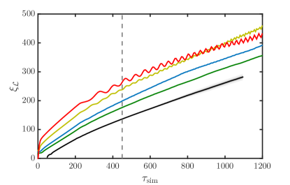
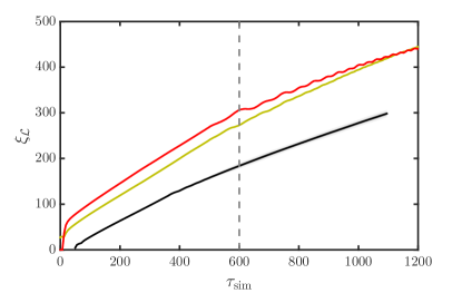
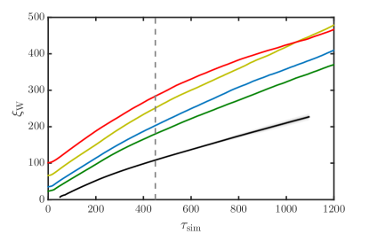
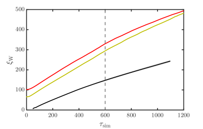
Figures 1 and 2 show the mean string separation estimated with two different measures: the total Lagrangian $\xi_{\mathcal{L}}$ and the winding measure $\xi_{\text{w}}$ respectively (see Eqs. (20) and (21)). Both figures include results from simulations in radiation dominated (top) and matter dominated backgrounds (bottom). The colour scheme is the following: red corresponds to $\beta=0.01$, yellow to $\beta=0.025$, blue to $\beta=0.1$, and green to $\beta=0.25$. As a reference $\beta=1$ from Daverio et al. (2016) is also added in black. In the figures we show a vertical line showing $\tau_{\mathrm{ref}}$. Times earlier than this are not used in the study of the network, since they are just an artifact of the initial conditions.The evidence of scaling happens for times later than $\tau_{\mathrm{ref}}$. The figures provide some evidence that all simulations are reaching scaling, as towards the end of the simulations the behaviour of $\xi$ is consistent with a linear increase with conformal time with similar slopes.

There are two phenomena worth mentioning: on the one hand, the mean string separation exhibits a late time attenuation for the lowest $\beta$, i.e. , $\beta=0.01$, visible in both radiation and matter, and in both different $\xi$ measures (as is evident in the curves intersecting ). On the other, the Lagrangian measure is oscillatory for $\beta=0.01$ (and to a lesser degree for $\beta=0.025$). The attenuation and the oscillations are caused by a poor choice of $\tau_{\mathrm{cg}}$ in the initial conditions (see discussion of Sec. III) which resulted in the scalar field executing coherent oscillations around its minimum.

However, visual inspection of the measures and comparison between $\xi_{\mathcal{L}}$ and $\xi_{\text{w}}$ show that the description of the evolution of the scaling regime can be equivalently described by both estimators.

This is also confirmed by checking the derivative of $\xi$ with respect to time. In Fig 3 we show the values obtained from the Lagrangian (blue) and winding (red) estimators. In order to account for the time variation of the slope, we calculate the average value of $\dot{\xi}$ over two different time ranges: intermediate times between 600 and 800 (depicted with a circles), and late times at the range between 1000 and 1200 (depicted with triangles), all in simulation units. This selection encompasses a sufficiently large time range so that the oscillations are averaged out. Fig 3 shows that the values given by both estimators are consistent and equivalent (and also shows the late time attenuation exhibited by $\beta=0.01$).

Figure 3: The rate of change with conformal time of the comoving mean string separation $\dot{\xi}$ for radiation and matter, using a winding (red) and Lagrangian (blue) weighted measures. The averages are calculated over times between 600 and 800 (depicted with a circles) and between 1000 and 1200 (depicted with triangles).

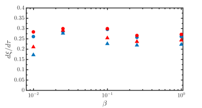
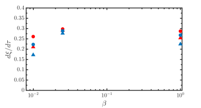
Cosmology	Radiation				Matter
$\beta$	0.01	0.025	0.1	0.25	0.01	0.025
$\tau_{\rm offset}$	-747.78	-387.01	-228.51	-238.16	-495.00	-284.52

Table 2: Values of $\tau_{\rm offset}$ for different simulations. All values obtained fitting $\xi$ over $\tau_{\text{sim}}\in[600\ 800]$.

Another measure of scaling can be obtained by the ratio of mean string separation to time. However, it is worth mentioning that in each simulation, the asymptotic linear behaviour has a time offset ($\tau_{\rm offset}$) due to the initial string density being somewhat lower than the scaling value, see Table 2 for specific values. (see Bevis et al. (2010) for a more detailed discussion). One could consider that the string network is scaling with respect to an internal time kept by the network itself, rather than $\tau_{\text{sim}}$, the time recorded in the simulation. The offset is larger for lower values of $\beta$ due to the higher initial string separation in these units. This internal time of the simulation can be estimated from the slopes of the mean string separation $\alpha=d\xi/d\tau$ (see Daverio et al. (2016)) according to

$$\tau=\tau_{\text{sim}}-\tau_{\rm offset}=\alpha^{-1}(\tau_{\text{sim}})\xi(\tau_{\text{sim}})\,.$$ (26)

Although in previous papers we used the Lagrangian estimator for this purpose, in this case we chose the winding estimator to avoid possible problems caused by the oscillations of the Lagrangian estimator.

Figure 4: Figures showing the ratio of the mean string separation to time for radiation (top) and matter (bottom) eras, using the winding estimate. The colour scheme is the same as in previous similar plots.

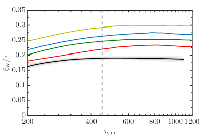
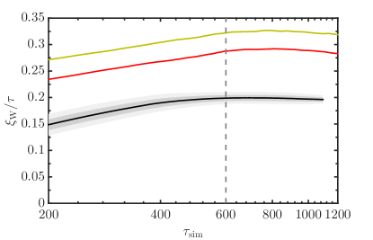
Using the winding estimator for the mean string separation and the internal time of the simulation, in Fig. 4 we show the ratio of the mean string separation to time ($\xi_{\text{w}}/\tau$), giving another indication of scaling.

The ETCs of the energy-momentum tensor (24) can also be used to estimate scaling. If the network scales, the ETCs from different stages of the simulation should collapse to a single line when plotted against $k\tau$. Using the definition of time given in (26), the $\xi$-scaled scaling ETCs read

$$E_{a}(k\tau,\beta)=\left(\frac{\tau}{\tau_{\text{sim}}}\right)E_{a}^{\rm(sim)}(k\tau_{\text{sim}},\beta),$$ (27)

where $\tau$ is the time as defined in Eq. (26), with $\xi$ and $\alpha$ determined from the winding measure. We represent simulation quantities with the subscript and superscript ‘sim’.

Figure 5: Complete set of ETCs from simulations in the radiation era. There are two sets of panels (a and b), each containing five different ETCs: on he left $E_{11}$, $E_{22}$ and $E_{12}$ from top to bottom, and on the right $E_{\text{vv}}$ and $E_{\text{tt}}$ from top to bottom. The a) panels show ETCs at their original amplitude, whereas the b) panels shows ETCs rescaled with the $\mu^{2}$ that corresponds to each $\beta$. The color scheme is as before: red for $\beta=0.01$, yellow for $\beta=0.025$, blue for $\beta=0.1$ green for $\beta=0.25$ and black for $\beta=1.0$. ETCs are extracted from $\tau_{\text{sim}}\in[600,700]$ for $\beta<1$ and $\tau_{\text{sim}}\in[450,600]$ for $\beta=1$. Within one colour, lighter shades correspond to earlier times.

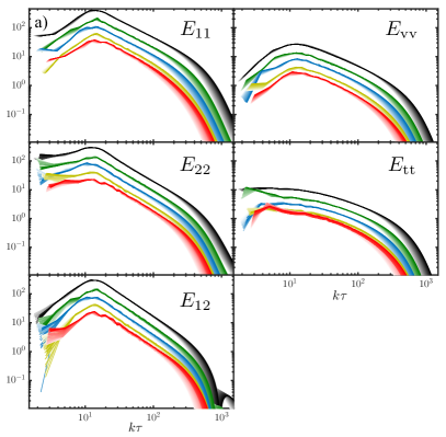
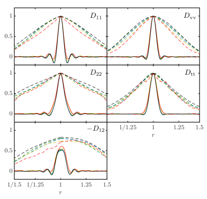
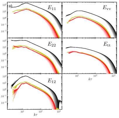
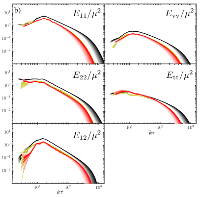
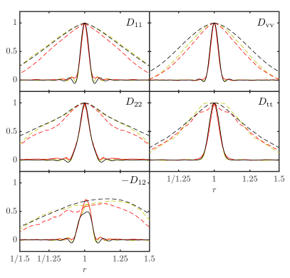
The complete set of ETCs for different $\beta$s can be found in panel “a)” of Fig. 5 for the radiation era. We also include the decoherence functions in Fig. 6 from radiation domination (see Appendix for the corresponding matter era figures). We maintain the same colour scheme as in previous figures.

The ETCs also provide evidence that for each case scaling has been reached. The shapes of the ETC for different values of $\beta$ seem similar, though lower values of $\beta$ correspond to lower values of the amplitude of the ETCs. Moreover, the differences in the values of the amplitudes are apparently shared between different ETCs. This difference could come from the different tension of the strings $\mu^{2}$. The decoherence functions also support this resemblance of the correlators of different simulations, indicating that the temporal decoherence of the UETCs is independent of $\beta$.

Figure 6: Complete set of decoherence function in radiation era. Five different functions are shown: on the left $D_{11}$, $D_{22}$ and $D_{21}$ from top to bottom, and on the right $D_{\text{vv}}$ and $D_{\text{tt}}$ from top to bottom. The colour scheme is maintained from previous plots: red for $\beta=0.01$, yellow for $\beta=0.025$, blue for $\beta=0.1$ green for $\beta=0.25$ and black for $\beta=1.0$. The decoherence functions are computed for $k\tau=10.5$ (dashed lines) and $k\tau=100$ (solid lines).

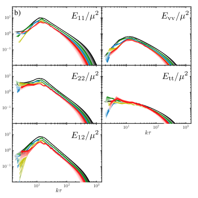
In order to account for the different energy-density scale of each one of the $\beta$, we calculated the ETCs dividing them by the value $\mu^{2}(\beta)$, computed using the formulae (10) and (II). The results can be found in the panel “b)” of Fig. 5 for radiation era (see Appendix for the corresponding matter era figure). The rescaling of the ETCs with $\mu^{2}$ brings the ETCs much closer to each other, almost lining them up (and for the tensor case, they do line up). However, there are still noticeable gaps between different $\beta$, a clear evidence that the different normalizations do not depend only on the string tension.

Nevertheless, it is interesting to note that even though the ETCs from simulations with higher $\beta$ are still above those with lower $\beta$, there is virtually no gap between the ETCs from the three lowest $\beta$. We interpret this as convergence of the $\mu^{2}$-rescaled ETCs at small $\beta$.

We calculate the extra factor needed to match the ETC from lowest $\beta$ to that given by the case with $\beta=1$, and call that factor $\kappa^{\rm R,M}$:

$$E^{\rm R,M}_{a}(k\tau,\beta)=\kappa_{a}^{\text{R,M}}\left(\frac{\mu(\beta)}{\mu(1)}\right)^{2}E^{\rm R,M}_{a}(k\tau,1)\,.$$ (28)

Table 3 contains the values of $\kappa$ for the whole set of simulations in radiation and in matter eras. In order to measure it, we fitted the region near the peak of the ETCs ($k\tau\in[9,60]$). We use the ETCs extracted at $\tau_{\text{sim}}=450$ and $\tau_{\text{sim}}=600$ for $\beta=1$ in radiation and matter respectively and $\tau_{\text{sim}}=660$ for $\beta<1$ simulations. The results from this procedure can be found in Table 3.

$\kappa_{a}^{\text{R}}$
$\beta$	$E_{11}$	$E_{22}$	$E_{12}$	$E_{\rm vv}$	Mean
0.01	0.65$\pm$0.06	0.53$\pm$0.05	0.57$\pm$0.05	0.63$\pm$0.03	0.59$\pm$0.09
0.025	0.58$\pm$0.03	0.51$\pm$0.03	0.55$\pm$0.03	0.58$\pm$0.02	0.56$\pm$0.05
0.1	0.64$\pm$0.02	0.59$\pm$0.03	0.62$\pm$0.03	0.67$\pm$0.02	0.63$\pm$0.05
0.25	0.86$\pm$0.03	0.84$\pm$0.03	0.84$\pm$0.03	0.86$\pm$0.02	0.85$\pm$0.05
$\kappa_{a}^{\text{M}}$
$\beta$	$E_{11}$	$E_{22}$	$E_{12}$	$E_{\rm vv}$	Mean
0.01	0.65$\pm$0.04	0.46$\pm$0.04	0.49$\pm$0.05	0.56$\pm$0.03	0.54$\pm$0.08
0.025	0.59$\pm$0.04	0.53$\pm$0.04	0.55$\pm$0.03	0.58$\pm$0.03	0.56$\pm$0.07

Table 3: Values of the extra normalization factor $\kappa_{a}^{\text{R,M}}$ for different correlators (except tensors) and different cosmologies R(adiation) and M(atter). The values are obtained by fitting for the region around the peak or maximum of the correlator ($k\tau\in[9,60]$) and for ETCs extracted at $\tau_{\text{sim}}=450$ and $\tau_{\text{sim}}=600$ ($\beta=1$) in radiation and matter respectively and $\tau_{\text{sim}}=660$ for $\beta<1$ simulations. Errors on each correlator come from averaging over the contribution of all bins in $k\tau\in[9,60]$.

Figure 7: Mean values and errors of the measure of $\kappa_{a}^{\text{R}}$ (blue) and $\kappa_{a}^{\text{M}}$ (red) as a function of $\beta$. The black dashed line corresponds to the function expressed in Eq. (29).

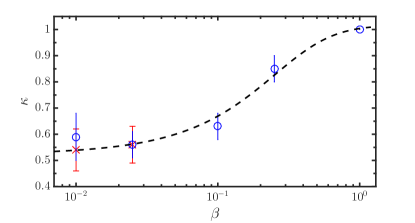
The mean points and the standard deviations for each $\beta$ are represented in Fig. 7, where we use blue for the data from radiation simulations and red for matter simulations. This figure shows that for the lowest $\beta$’s the value of the factor seems to tend to an asymptote. We obtained an analytical expression for $\kappa(\beta)$ fitting those points and using the following function:

$$\kappa(\beta)=\kappa_{0}+a\tanh(b\log(\beta+1))\quad(\beta<1),$$ (29)

where: $a=0.49\pm 0.05$, $b=7.4\pm 1.6$ and $\kappa_{0}=0.52\pm 0.03$.

This is the functional form for interpolation for different values of $\beta$. The asymptotic value for any arbitrarily low $\beta$ is, therefore, $\kappa_{0}=0.52\pm 0.03$, which is within $1\sigma$ confidence-limit of our measurement for our lowest $\beta$ simulations, suggesting that the $\kappa(\beta)$ correction for lower values of $\beta$ is of $O(1)$. Tensor correlators do not require any extra normalization beyond $\mu^{2}$, and it is consistent to take $\kappa^{\text{R,M}}_{\text{tt}}=1$.

V $C_{\ell}$ and constraints

Obtaining the CMB anisotropies power spectra from strings is rather involved. The procedure and high resolution $C_{\ell}$’s from $4096^{3}$ simulations at $\beta=1$ can be found in Lizarraga et al. (2016).

The fact that the ETCs from different $\beta$ are (almost) a rescaled version of each other prompts us to provide a recipe to give an approximate CMB anisotropies power spectra from strings at any $\beta$ $(<1)$, by using the aforementioned high resolution $C_{\ell}$’s from $\beta=1$ Lizarraga et al. (2016), rather than having to compute the $C_{\ell}$’s for every different $\beta$.

The CMB power spectra from strings are linear responses to the unequal time correlators (UETCs) (22). In the previous section we demonstrated that, to a good approximation, the UETCs at low $\beta$ can be obtained by rescaled those at $\beta=1$. Thus, our claim is that the $C_{\ell}$s for a given $\beta$ can be obtained by just rescaling the $C_{\ell}$s at $\beta=1$ Lizarraga et al. (2016). Given the different scaling properties of the tensor source, this rescaling should be performed separately for the scalar, vector and tensor perturbation modes, or

$$C^{\text{L}}_{\ell}(\beta)=\kappa^{\text{L}}(\beta)\left(\frac{\mu(\beta)}{\mu(1)}\right)^{2}C^{\text{L}}_{\ell}(1)\,,$$ (30)

where $L=S,V,T$ and

$$\kappa^{\text{S,V}}(\beta) = \kappa(\beta)$$ (31)

$$\kappa^{\text{T}}(\beta) = 1.$$ (32)

We recall that the function $\kappa(\beta)$ is given in Eq. (29), and $\mu(\beta)/\mu(1)=B(\beta)$, which is approximated in (II). We can then estimate the CMB constraints to any $\beta<1$.

So far the constraints imposed by CMB experiments, such as Planck, in the abundance of cosmic strings come from channels (TT, TE and EE) where tensor modes are the least dominant. Therefore, it is reasonable to assume that the entire normalisation difference can be encapsulated in $\kappa(\beta)=\kappa^{\text{S,V}}(\beta)$, and that the mismatch with $\kappa^{\text{T}}$ produces a negligible effect in the new constraints.

For example, we can obtain the constraints in $G\mu$ for Planck 2015 as a function of $\beta$, by just extrapolating our $\beta=1$ results Lizarraga et al. (2016), which imply that $\kappa^{1/2}(\beta)G\mu(\beta)\lesssim 2.0\times 10^{-7}$. Oour results suggest that $\kappa(\beta)$ would be of order $O(1)$ for lower values of $\beta$. This information can be recast into obtaining constraints for the energy scale of the symmetry breaking $\phi_{0}$ as a function of $\beta$:

$$\phi_{0}\kappa(\beta)^{1/4} \lesssim B(\beta)^{-1/2}2.2\times 10^{15}\,\text{GeV}\,,$$ (33)

with $\kappa(\beta)\sim O(1)$ for very low $\beta$. This shows that models with low $\beta$ would allow higher symmetry-breaking scales to be compatible with the constraints on strings from the CMB.

VI Conclusion and Discussion

In this paper we have presented the first network simulations of the Abelian Higgs model for $\beta<1$ to include both matter and radiation eras and Cosmic Microwave Background (CMB) constraints. The comoving mean string separation $\xi(\tau)$ is found to grow in a manner consistent with linear, giving evidence that the strings are scaling as usual. The dependence of the growth rate $d\xi/d\tau$ on $\beta$ is weak, and consistent with it being independent of $\beta$. The lack of dependence of $d\xi/d\tau$ on $\beta$ is more evidence that the radiative energy-loss mechanism studied in Hindmarsh et al. (2017) is non-perturbative: perturbative scalar radiation should decrease with the scalar self-coupling $\lambda$ and hence $\beta$.

Our result for the mean string separation differs from that of Hiramatsu et al. (2013), who found that the mean string separation towards the end of the simulations reached a minimum at $\beta=0.4$, and increased again at the lowest $\beta$ achieved, $\beta=0.2$. Our initial conditions are prepared with a period of cooling to remove short-distance oscillations and bring the scalar field as close as possible to its minimum, consistent with there being a string network. The simulations of Hiramatsu et al. (2013) on the other hand do not have cooling, and show signs of a coherent oscillation of the scalar field, which affects the string length measurement. Our simulations also reach string separations which are significantly larger. We therefore agree with the tentative conclusions of Hiramatsu et al. (2013) that the apparent $\beta$-dependence of the string separation should disappear for larger simulations.

The stress-energy correlators $C_{ab}$ on the other hand do depend on $\beta$. This dependence is well described by a simple rescaling with the string mass with the string tension $\mu$, $C_{ab}\propto(\mu(\beta)/\mu(1))^{2}$, except for an additional O(1) correction that we call $\kappa$, as given in Eq. (28). We measure this correction factor in our simulations and find that the values for all UETCs except for the tensors are comparable. A functional fit to our measured $\kappa$ values for any $\beta$ is given in Eq. (29) showing that for $\beta\lesssim 0.1$ it asymptotes to $\kappa_{0}=0.52\pm 0.03$, suggesting $\kappa~{}O(1)$ for very low values of $\beta$. For the tensor-type stress-energy UETCs we find no additional correction, i.e. $\kappa_{tt}\simeq 1$. As the tensor UETCs do not depend on $T^{0i}$, while the other UETCs do, we conjecture that the correction factor, which encodes the effect of the string interactions when $\beta\neq 1$, may reflect that networks with lower values $\beta$ have slightly smaller velocities.

The simple scaling of the scalar and vector UETCs implies that also the angular power spectrum of temperature fluctuations $C^{TT}_{\ell}$ is simply rescaled by the same factor, given in Eq. (30), as the tensor UETCs contribute to the temperature fluctuations only at a low level. This equation allows to predict the CMB angular anisotropy power spectra for any $\beta<1$. Because of this rescaling, models with low (effective) self-coupling can satisfy the CMB bounds at higher symmetry-breaking scales.

If our results can be extrapolated to very low $\beta$, they would allow higher symmetry-breaking scales to be compatible with the constraints on strings from the CMB. This is particularly relevant for models where the symmetry is broken along a flat direction lifted by supersymmetry-breaking terms Lazarides et al. (1987), which can have effective values of $\beta$ in the range $10^{-30}\lesssim\beta\lesssim 10^{-15}$ Cui et al. (2008). The supersymmetric F-term hybrid inflation model of Hindmarsh and Jones (2013) has $\beta_{\text{eff}}\sim 10^{-24}$, and so $B\simeq 0.04$. When normalised to the amplitude of inflationary perturbations, it is found that $G\mu\simeq 10^{-7}$, compatible with current CMB constraints. Strings formed at $10^{16}$ GeV (around the supersymmetric GUT scale) would be allowed if $\beta\lesssim 10^{-15}$, although to reach $2\times 10^{16}$ GeV would need $\beta\lesssim 10^{-62}$. Such low-$\beta$ models must also find ways to avoid the complementary $\gamma$-ray Santana Mota and Hindmarsh (2015) or gravitational wave Ringeval and Suyama (2017); Blanco-Pillado et al. (2018) constraints. One possibility is that the string network decays entirely into particles in a hidden sector.

Appendix A Results from matter-era simulations

Here we show the equal time correlators (Fig. 8) and decoherence functions (Fig. 9) from the three matter era simulations, which complement the radiation era data show in Figs. 5, 6. The parameters of the runs are given in Table 1.

Figure 8: As Fig. 5 but with the ETCs from matter domination. ETCs are extracted from $\tau_{\text{sim}}\in[600,700]$ for $\beta<1$ and $\tau_{\text{sim}}\in[600,750]$ for $\beta=1$.

Figure 9: Complete set of decoherence function in matter era. Five different functions are shown: on the left $D_{11}$, $D_{22}$ and $D_{21}$ from top to bottom, and on the right $D_{\text{vv}}$ and $D_{\text{tt}}$ from top to bottom. The colour scheme is maintained from previous plots: red for $\beta=0.01$, yellow for $\beta=0.025$, blue for $\beta=0.1$ green for $\beta=0.25$ and black for $\beta=1.0$. The decoherence functions are computed for $k\tau=10.5$ (dashed lines) and $k\tau=100$ (solid lines).

References

- Kibble (1976) T. Kibble, J.Phys. A9, 1387 (1976).
- Vilenkin and Shellard (1994) A. Vilenkin and E. Shellard, Cosmic strings and other topological defects (Cambridge University Press, 1994).
- Jeannerot et al. (2003) R. Jeannerot, J. Rocher, and M. Sakellariadou, Phys.Rev. D68, 103514 (2003), eprint hep-ph/0308134.
- Zeldovich (1980) Ya. B. Zeldovich, Mon. Not. Roy. Astron. Soc. 192, 663 (1980).
- Vilenkin (1981a) A. Vilenkin, Phys.Rev.Lett. 46, 1169 (1981a).
- Hindmarsh and Kibble (1995) M. Hindmarsh and T. Kibble, Rept.Prog.Phys. 58, 477 (1995), eprint hep-ph/9411342.
- Sakellariadou (2007) M. Sakellariadou, Lect.Notes Phys. 718, 247 (2007), eprint hep-th/0602276.
- Copeland et al. (2011) E. J. Copeland, L. Pogosian, and T. Vachaspati, Class.Quant.Grav. 28, 204009 (2011), eprint 1105.0207.
- Hindmarsh (2011) M. Hindmarsh, Prog.Theor.Phys.Suppl. 190, 197 (2011), eprint 1106.0391.
- Gott (1985) I. Gott, J. Richard, Astrophys.J. 288, 422 (1985).
- Kaiser and Stebbins (1984) N. Kaiser and A. Stebbins, Nature 310, 391 (1984).
- Vilenkin (1981b) A. Vilenkin, Phys.Lett. B107, 47 (1981b).
- Hogan and Rees (1984) C. Hogan and M. Rees, Nature 311, 109 (1984).
- Sigl et al. (1995) G. Sigl, K. Jedamzik, D. Schramm, and V. Berezinsky, Phys.Rev. D52, 6682 (1995), eprint astro-ph/9503094.
- Protheroe and Stanev (1996) R. Protheroe and T. Stanev, Phys.Rev.Lett. 77, 3708 (1996), eprint astro-ph/9605036.
- Matsunami et al. (2019) D. Matsunami, L. Pogosian, A. Saurabh, and T. Vachaspati (2019), eprint 1903.05102.
- Ringeval and Suyama (2017) C. Ringeval and T. Suyama, JCAP 1712, 027 (2017), eprint 1709.03845.
- Blanco-Pillado et al. (2018) J. J. Blanco-Pillado, K. D. Olum, and X. Siemens, Phys. Lett. B778, 392 (2018), eprint 1709.02434.
- Santana Mota and Hindmarsh (2015) H. F. Santana Mota and M. Hindmarsh, Phys. Rev. D91, 043001 (2015), eprint 1407.3599.
- Nielsen and Olesen (1973) H. B. Nielsen and P. Olesen, Nucl.Phys. B61, 45 (1973).
- Bevis et al. (2008) N. Bevis, M. Hindmarsh, M. Kunz, and J. Urrestilla, Phys.Rev.Lett. 100, 021301 (2008), eprint astro-ph/0702223.
- Ade et al. (2014) P. Ade et al. (Planck Collaboration), Astron.Astrophys. 571, A25 (2014), eprint 1303.5085.
- Lizarraga et al. (2014) J. Lizarraga, J. Urrestilla, D. Daverio, M. Hindmarsh, M. Kunz, and A. R. Liddle, Phys. Rev. D90, 103504 (2014), eprint 1408.4126.
- Ade et al. (2016) P. A. R. Ade et al. (Planck), Astron. Astrophys. 594, A13 (2016), eprint 1502.01589.
- Lizarraga et al. (2016) J. Lizarraga, J. Urrestilla, D. Daverio, M. Hindmarsh, and M. Kunz, JCAP 1610, 042 (2016), eprint 1609.03386.
- Lazanu and Shellard (2015) A. Lazanu and P. Shellard, JCAP 1502, 024 (2015), eprint 1410.5046.
- Charnock et al. (2016) T. Charnock, A. Avgoustidis, E. J. Copeland, and A. Moss, Phys. Rev. D93, 123503 (2016), eprint 1603.01275.
- Battye et al. (2010) R. Battye, B. Garbrecht, and A. Moss, Phys.Rev. D81, 123512 (2010), eprint 1001.0769.
- Hill et al. (1988) C. T. Hill, H. M. Hodges, and M. S. Turner, Phys.Rev. D37, 263 (1988).
- Lazarides et al. (1987) G. Lazarides, C. Panagiotakopoulos, and Q. Shafi, Phys. Lett. B183, 289 (1987).
- Perkins and Davis (1998) W. B. Perkins and A.-C. Davis, Phys. Lett. B428, 254 (1998), eprint hep-ph/9803303.
- Cui et al. (2008) Y. Cui, S. P. Martin, D. E. Morrissey, and J. D. Wells, Phys. Rev. D77, 043528 (2008), eprint 0709.0950.
- Hindmarsh and Jones (2013) M. Hindmarsh and D. R. T. Jones, Phys. Rev. D87, 075022 (2013), eprint 1203.6838.
- Bogomolnyi (1976) E. B. Bogomolnyi, Sov. J. Nucl. Phys. 24, 449 (1976).
- Achúcarro and de Putter (2006) A. Achúcarro and R. de Putter, Phys.Rev. D74, 121701 (2006), eprint hep-th/0605084.
- Verbiest and Achucarro (2011) G. J. Verbiest and A. Achucarro, Phys. Rev. D84, 105036 (2011), eprint 1106.4666.
- Hiramatsu et al. (2013) T. Hiramatsu, Y. Sendouda, K. Takahashi, D. Yamauchi, and C.-M. Yoo, Phys. Rev. D88, 085021 (2013), eprint 1307.0308.
- Bogomolnyi and Vainshtein (1976) E. B. Bogomolnyi and A. Vainshtein, Sov. J. Nucl. Phys. 23, 588 (1976).
- Manton and Sutcliffe (2007) N. S. Manton and P. Sutcliffe, Topological solitons (Cambridge University Press, 2007), ISBN 9780521040969, 9780521838368, 9780511207839, URL http://www.cambridge.org/uk/catalogue/catalogue.asp?isbn=0521838363.
- Press et al. (1989) W. H. Press, B. S. Ryden, and D. N. Spergel, Astrophys. J. 347, 590 (1989).
- Bevis et al. (2007a) N. Bevis, M. Hindmarsh, M. Kunz, and J. Urrestilla, Phys.Rev. D75, 065015 (2007a), eprint astro-ph/0605018.
- Bevis et al. (2007b) N. Bevis, M. Hindmarsh, M. Kunz, and J. Urrestilla, Phys.Rev. D76, 043005 (2007b), eprint 0704.3800.
- Hindmarsh et al. (2017) M. Hindmarsh, J. Lizarraga, J. Urrestilla, D. Daverio, and M. Kunz, Phys. Rev. D96, 023525 (2017), eprint 1703.06696.
- Kajantie et al. (1998) K. Kajantie, M. Karjalainen, M. Laine, J. Peisa, and A. Rajantie, Phys.Lett. B428, 334 (1998), eprint hep-ph/9803367.
- Scherrer and Vilenkin (1998) R. J. Scherrer and A. Vilenkin, Phys.Rev. D58, 103501 (1998), eprint hep-ph/9709498.
- Bevis et al. (2010) N. Bevis, M. Hindmarsh, M. Kunz, and J. Urrestilla, Phys.Rev. D82, 065004 (2010), eprint 1005.2663.
- Daverio et al. (2016) D. Daverio, M. Hindmarsh, M. Kunz, J. Lizarraga, and J. Urrestilla, Phys. Rev. D93, 085014 (2016), [Erratum: Phys. Rev.D95,no.4,049903(2017)], eprint 1510.05006.