A recursive distribution equation for the stable tree

Abstract

We provide a new characterisation of Duquesne and Le Gall’s $\alpha$-stable tree, $\alpha\!\in\!(1,2]$,as the solution of a recursive distribution equation (RDE) of the form $\mathcal{T}\!\overset{d}{=}\!g\left(\xi,\!\mathcal{T}_{i},i\!\geq\!0\right)$, where $g$ is a concatenation operator, $\xi=\left(\xi_{i},i\geq 0\right)$ a sequence of scaling factors, $\mathcal{T}_{i}$, $i\geq 0$, and $\mathcal{T}$ are i.i.d. trees independent of $\xi$. This generalises a version of the well-known characterisation of the Brownian Continuum Random Tree due to Aldous, Albenque and Goldschmidt. By relating to previous results on a rather different class of RDE, we explore the present RDE and obtain for a large class of similar RDEs that the fixpoint is unique (up to multiplication by a constant) and attractive.

Keywords: Recursive distribution equation; $\mathbb{R}$-tree; Gromov–Hausdorff distance; stable tree

AMS subject classification: 60J80; 60J05.

1 Introduction

$\mathbb{R}$-trees, constitute a class of loop-free length spaces which frequently arise as scaling limits of many discrete trees [25]. In their own right, $\mathbb{R}$-trees have diverse applications from rough path integration theory [36] to phylogenetic models [32]. Following Aldous’s introduction of the Brownian Continuum Random Tree (BCRT) [5, 6, 7], significant attention turned to random $\mathbb{R}$-trees. Naturally, the BCRT manifests in the asymptotics of discrete tree-like structures, including uniform random labelled trees [5, 7] and critical Galton–Watson trees with finite offspring variance [5]. Bewilderingly, recent applications of the BCRT have surpassed objects not overtly tree-like, for example, random recursive triangulations [21], random planar quadrangulations [44], and Liouville quantum gravity [23].

The BCRT was generalised by Duquesne and Le Gall’s $\alpha$-stable trees [27, 28], parameterised by $\alpha\in(1,2]$. The $\alpha$-stable trees are themselves a special case of Le Gall and Le Jan’s Lévy trees [38], representing the genealogies of continuous-state branching processes with branching mechanism $\psi(\lambda)=\lambda^{\alpha}$. When $\alpha=2$, we recover the BCRT. Akin to the BCRT, the family of $\alpha$-stable trees constitutes all possible scaling limits of Galton–Watson trees, conditioned on the total progeny, whose offspring distribution lies in the domain of attraction of an $\alpha$-stable law [24]. Likewise, $\alpha$-stable trees emerge in scaling limits of numerous discrete tree structures, e.g., vertex-cut Galton–Watson trees [22] and conditioned stable Lévy forests [16]. Pursuing a dedicated approach with Lévy processes gives links to superprocesses [27, 38], and beta-coalescents in genetic models [1, 11]. Particular aspects of $\alpha$-stable trees, such as, invariance under uniform re-rooting [35], Hausdorff and packing measures [26, 29, 28], spectral dimensions [19], heights and diameters [30], and an embedding property of stable trees [20], have also been closely studied.

We wish to emphasise a crucial self-similarity property of $\alpha$-stable trees. This property plausibly explains the prevalence of $\alpha$-stable trees in such diverse contexts, especially in problems of a recursive nature. Decomposing an $\alpha$-stable tree above a certain height or at appropriate nodes results in the connected components after decomposition forming rescaled independent copies of the original tree. This observation was first formalised by Miermont [41, 42], building upon Bertoin’s self-similar fragmentation theory [12].

In this paper, we express the self-similarity of the $\alpha$-stable tree by a new recursive distribution equation (RDE) in the setting of Aldous and Bandyopadhyay’s survey paper [9]. Given a random variable $\mathcal{T}$ valued in a Polish metric space $(\mathbb{T},d)$, an RDE is a stochastic equation of the form

$$\mathcal{T}\overset{d}{=}g\left(\xi,\mathcal{T}_{i},i\geq 0\right)\quad\textnormal{ on }\mathbb{T},$$

where $(\mathcal{T}_{i},i\geq 0)$ are i.i.d. and distributed as $\mathcal{T}$, $g$ is a measurable mapping, and $\xi$ is independent of $\left(\mathcal{T}_{i},i\geq 0\right)$. RDEs are pertinent in various contexts with recursive structures, including Galton–Watson branching processes [9], Poisson weighted infinite trees [10], and Quicksort algorithms [51].

RDEs have been employed in the recursive construction of the BCRT by Albenque and Goldschmidt [4], recursively concatenating three rescaled trees at a single point. Broutin and Sulzbach [14] extended this to further recursive combinatorial structures and weighted $\mathbb{R}$-trees under a finite concatenation operation. Rembart and Winkel [49] did similarly with $\mathbb{R}$-trees under a different operation that concatenates a countable (possibly infinite) number of rescaled trees to a branch/spine. See Figure 1.

   

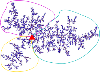
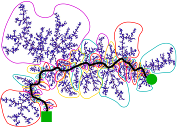
Figure 1: RDEs derived from the decomposition of the BCRT (simulation courtesy of Igor Kortchemski) around a branchpoint (the red triangle) into three parts and along the spine from the root (green square) to a random leaf (green circle) into “infinitely many” parts.

In this paper, we consider as $g$ the operation that concatenates at a single point a countable number of $\mathbb{R}$-trees $\mathcal{T}_{i}\overset{d}{=}\mathcal{T}$, rescaled by $\xi_{i}\geq 0$, $i\geq 0$, respectively, seeking to obtain a version of $\mathcal{T}$. Theorem 3.8 shows that the law of the $\alpha$-stable tree is a fixpoint solution of an RDE of this type. This is illustrated in Figure 2. Our primary argument appeals to Marchal’s random growth algorithm [40], which provides a recursive method of constructing $\alpha$-stable trees as a scaling limit. To explore the uniqueness of this solution (up to rescaling distances by a constant) we first observe that we require certain finite height moments. In the absence of this condition, further solutions can be obtained, for example, by decorating the $\alpha$-stable tree with massless branches, see Remark 3.9.

   

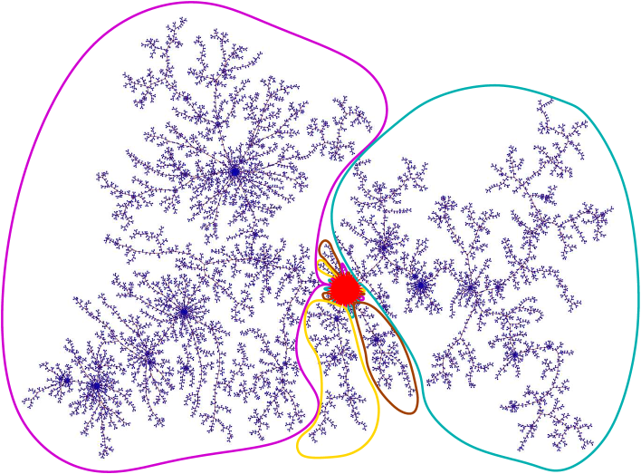
Figure 2: RDEs derived from the decomposition of a stable tree (simulation courtesy of Igor Kortchemski) around a branchpoint (the red star) into “infinitely many” parts.

Let us explore our approach to uniqueness and attraction in the context of the literature. While our results closely resemble [4] and [14] for the (binary) BCRT and other finitely branching structures, our methods are rather different. Indeed, our results extend finite concatenation operations to handle trees such as the $\alpha$-stable trees, whose branch points are of countably infinite multiplicity. Extending their uniqueness and attraction results is not straightforward using the methods of [4, 14]. On the other hand, [49] presents an RDE for which the law of the $\alpha$-stable tree is a unique and attractive fixpoint, but the concatenation approach of employing strings of beads (weighted intervals) and bead-splitting processes of [47] is different. Our RDEs only require countably infinite weight sequences such as Poisson–Dirichlet sequences and gives a less technical recursive construction of $\alpha$-stable trees that elucidates how mass partitions in $\alpha$-stable trees relate to urn models and partition-valued processes.

Specifically, we prove the self-similarity property of $\alpha$-stable trees decomposed at a branch point solely via the recursive nature of Marchal’s algorithm, without need for Miermont’s fragmentation tree theory [42]. To prove our uniqueness and attraction result, Theorem 4.2, we establish a connection between the two types of RDE, which effectively breaks down the proofs here into a one-dimensional martingale argument, the uniqueness and attraction of the RDE of [49] and a tightness argument that again builds on [49] by constructing an auxiliary dominating CRT.

The structure of this paper is as follows. In Section 2, we state background results on $\mathbb{R}$-trees and $\alpha$-stable trees and collect tools required to obtain our results, namely the rigorous setup of RDEs, Pólya urn models, the Chinese restaurant process and Marchal’s algorithm. Section 3 is dedicated to establishing an RDE for the law of the $\alpha$-stable tree and indicating other fixpoint solutions to the same RDE. In Section 4, we obtain the uniqueness and attraction properties of the RDE solution up to multiplicative constants. The latter arguments are in a general setup where $g$ is the single-point concatenation operation, but the distribution of $\xi$ is just subject to some non-degeneracy assumptions.

2 Preliminaries

We introduce several background formalisms and theories on metric spaces of $\mathbb{R}$-trees, $\alpha$-stable trees, urn schemes and recursive distribution equations. We also state a general lemma that we will use to establish independence.

2.1 $\mathbb{R}$-trees and topologies on sets of (weighted or marked) $\mathbb{R}$-trees

Definition 2.1 ($\mathbb{R}$-tree)

A metric space $\left(\mathcal{T},d\right)$ is an $\mathbb{R}$-tree if for every $a,b\in\mathcal{T}$, the following two conditions hold.

• There exists a unique isometry $f_{a,b}\colon\left[0,d(a,b)\right]\rightarrow\mathcal{T}$ such that $f_{a,b}(0)=a$ and $f_{a,b}(d(a,b))=b$. In this case, let $\llbracket a,b\rrbracket$ denote the image $f_{a,b}\left(\left[0,d(a,b)\right]\right)$.

• If $h\colon\left[0,1\right]\rightarrow\mathcal{T}$ is a continuous injective map with $h\left(0\right)=a$ and $h\left(1\right)=b$, then $h\left(\left[0,1\right]\right)=\llbracket a,b\rrbracket$, i.e. the only non self-intersecting path from $a$ to $b$ is $\llbracket a,b\rrbracket$.

A rooted $\mathbb{R}$-tree $(\mathcal{T},d,\rho)$ is an $\mathbb{R}$-tree $(\mathcal{T},d)$ with a distinguished vertex $\rho\in\mathcal{T}$ called the root. The degree of a vertex $a\in\mathcal{T}$ is the number of connected components of $\mathcal{T}\setminus\{a\}$. A leaf is a vertex $a\in\mathcal{T}\setminus\{\rho\}$ with degree one. We denote the set of leaves in $\mathcal{T}$ by $\mathcal{L}\left(\mathcal{T}\right)$. We say that $a\in\mathcal{T}\setminus\{\rho\}$ is a branch point if its degree is at least three. Finally, for any $a\in\mathcal{T}$, we define the height of $a$ as $d\left(\rho,a\right)$, and the height of $\mathcal{T}$ as $\textnormal{ht}\left(\mathcal{T}\right):=\sup_{a\in\mathcal{T}}d\left(\rho,a\right)$.

Two rooted $\mathbb{R}$-trees $\left(\mathcal{T},d,\rho\right)$ and $\left(\mathcal{T}^{\prime},d^{\prime},\rho^{\prime}\right)$ are GH-equivalent if there exists an isometry $f\colon\mathcal{T}\rightarrow\mathcal{T}^{\prime}$ such that $f\left(\rho\right)=\rho^{\prime}$. The set of GH-equivalence classes of compact rooted $\mathbb{R}$-trees is denoted by $\mathbb{T}$. The Gromov–Hausdorff distance between two rooted compact $\mathbb{R}$-trees $\left(\mathcal{T},d,\rho\right)$ and $\left(\mathcal{T}^{\prime},d^{\prime},\rho^{\prime}\right)$ is defined as

$$d_{\rm GH}((\mathcal{T},d,\rho),(\mathcal{T}^{\prime},d^{\prime},\rho^{\prime})):=\inf_{\phi,\phi^{\prime}}\left(\delta_{\rm H}(\phi(\mathcal{T}),\phi^{\prime}(\mathcal{T}^{\prime}))\vee\delta(\phi(\rho),\phi^{\prime}(\rho^{\prime}))\right)$$ (1)

where the infimum is taken over all metric spaces $\left(X,\delta\right)$ and all isometric embeddings $\phi\colon\mathcal{T}\rightarrow X$ and $\phi^{\prime}\colon\mathcal{T}^{\prime}\rightarrow X$, and where $\delta_{\rm H}$ is the Hausdorff metric on compact subsets of $(X,\delta)$. The Gromov–Hausdorff distance only depends on the GH-equivalence classes of $\left(\mathcal{T},d,\rho\right)$ and $\left(\mathcal{T}^{\prime},d^{\prime},\rho^{\prime}\right)$ and induces a metric on $\mathbb{T}$, which we also denote by $d_{\rm GH}$.

There is an alternative characterisation of the Gromov–Hausdorff metric [15, Theorem 7.3.25]. Given two compact metric spaces $(X,\delta)$ and $(X^{\prime},\delta^{\prime})$, a correspondence between $X$ and $X^{\prime}$ is a subset $\mathcal{R}\subseteq X\times X^{\prime}$ such that for every $x\in X$, there exists at least one $x^{\prime}\in X^{\prime}$ such that $(x,x^{\prime})\in\mathcal{R}$, and conversely, for every $y^{\prime}\in X^{\prime}$, there exists at least one $y\in X$ such that $(y,y^{\prime})\in\mathcal{R}$. The distortion of this correspondence $\mathcal{R}$ is defined as

$$\textnormal{dis}(\mathcal{R}):=\sup\big{\{}\left|\delta(x,y)-\delta^{\prime}(x^{\prime},y^{\prime})\right|\colon(x,x^{\prime}),(y,y^{\prime})\in\mathcal{R}\big{\}}.$$ (2)

In our setting of two compact rooted $\mathbb{R}$-trees $\left(\mathcal{T},d,\rho\right)$ and $\left(\mathcal{T}^{\prime},d^{\prime},\rho^{\prime}\right)$, we obtain

$$d_{\rm GH}\left(\left(\mathcal{T},d,\rho\right),\left(\mathcal{T}^{\prime},d^{\prime},\rho^{\prime}\right)\right)=\frac{1}{2}\displaystyle\inf_{\mathcal{R}\in\mathcal{C}\left(\mathcal{T},\mathcal{T}^{\prime}\right)}\text{dis}\left(\mathcal{R}\right),$$ (3)

where $\mathcal{C}(\mathcal{T},\mathcal{T}^{\prime})$ is the set of all correspondences $\mathcal{R}$ between $(\mathcal{T},d,\rho)$ and $(\mathcal{T}^{\prime},d^{\prime},\rho^{\prime})$ which have $(\rho,\rho^{\prime})$ in correspondence, i.e. for which $(\rho,\rho^{\prime})\in\mathcal{R}$.

We will want to specify a marked point on a compact rooted $\mathbb{R}$-tree. We refer the reader to [43, Section 6.4] for further extensions. Given two marked compact rooted $\mathbb{R}$-trees $\left(\mathcal{T},d,\rho,x\right)$ and $\left(\mathcal{T^{\prime}},d^{\prime},\rho^{\prime},x^{\prime}\right)$, the marked Gromov–Hausdorff distance is defined as

$$d_{\rm GH}^{\rm m}\!\left(\!\left(\mathcal{T}\!,d,\rho,x\right)\!,\left(\mathcal{T^{\prime}}\!,d^{\prime}\!,\rho^{\prime}\!,x^{\prime}\right)\!\right):=\inf_{\phi,\phi^{\prime}}\!\left(\delta_{\rm H}\!\left(\phi\!\left(\mathcal{T}\right)\!,\phi^{\prime}\!\left(\mathcal{T}^{\prime}\right)\right)\vee\delta\!\left(\phi\!\left(\rho\right)\!,\phi^{\prime}\!\left(\rho^{\prime}\right)\right)\vee\delta\!\left(\phi\!\left(x\right),\phi^{\prime}\!(x^{\prime})\right)\right),$$

where the infimum is taken over all metric spaces $\left(X,\delta\right)$ and all isometric embeddings $\phi\colon\mathcal{T}\rightarrow X$ and $\phi^{\prime}\colon\mathcal{T}^{\prime}\rightarrow X$. We say two marked compact rooted $\mathbb{R}$-trees are ${\rm GH}^{\rm m}$-equivalent if there exists an isometry $f\colon\mathcal{T}\rightarrow\mathcal{T}^{\prime}$ such that $f(\rho)=\rho^{\prime}$ and $f(x)=x^{\prime}$. We denote the set of equivalence classes of marked compact rooted $\mathbb{R}$-trees by $\mathbb{T}_{\rm m}$. The marked Gromov–Hausdorff distance only depends on the ${\rm GH}^{\rm m}$-equivalence classes of $\left(\mathcal{T},d,\rho,x\right)$ and induces a metric on $\mathbb{T}_{\rm m}$, which we also denote by $d^{\rm m}_{\rm GH}$. In the spirit of (3), we obtain for marked compact rooted $\mathbb{R}$-trees $(\mathcal{T},d,\rho,x)$ and $(\mathcal{T}^{\prime},d^{\prime},\rho^{\prime},x^{\prime})$,

$$d_{\rm GH}^{\rm m}\left(\left(\mathcal{T},d,\rho,x\right),\left(\mathcal{T}^{\prime},d^{\prime},\rho^{\prime},x^{\prime}\right)\right)=\frac{1}{2}\displaystyle\inf_{\mathcal{R}\in\mathcal{C}^{\rm m}\left(\mathcal{T},\mathcal{T}^{\prime}\right)}\text{dis}\left(\mathcal{R}\right).$$ (4)

where we denote by $\mathcal{C}^{\rm m}(\mathcal{T},\mathcal{T}^{\prime})$ the set of all correspondences between $(\mathcal{T},d,\rho,x)$ and $(\mathcal{T}^{\prime},d^{\prime},\rho^{\prime},x^{\prime})$ which have $(\rho,\rho^{\prime})$ and $(x,x^{\prime})$ in correspondence; cf. [43, Proposition 9(i)].

Suppose now that $(X,\delta)$ is a complete metric space. Then $\left(X,\delta,\mu\right)$ is a metric measure space if $(X,\delta)$ is further equipped with a Borel probability measure $\mu$. We define a weighted $\mathbb{R}$-tree as a compact rooted $\mathbb{R}$-tree $\left(\mathcal{T},d,\rho\right)$ equipped with a Borel probability measure $\mu$, which we refer to as mass measure. We will often write $\mathcal{T}$ for a weighted $\mathbb{R}$-tree, the distance, the root and the mass measure being implicit. For two weighted $\mathbb{R}$-trees $\left(\mathcal{T},d,\rho,\mu\right)$, $\left(\mathcal{T}^{\prime},d^{\prime},\rho^{\prime},\mu^{\prime}\right)$, the Gromov–Hausdorff–Prokhorov distance is defined as

$$d_{\rm GHP}((\mathcal{T}\!,d,\rho,\mu),(\mathcal{T}^{\prime}\!,d^{\prime}\!,\rho^{\prime}\!,\mu^{\prime})):=\inf_{\phi,\phi^{\prime}}\left(\delta_{\rm H}(\phi(\mathcal{T}),\phi^{\prime}(\mathcal{T}^{\prime}))\vee\delta(\phi(\rho),\phi^{\prime}(\rho^{\prime}))\vee\delta_{\rm P}(\phi_{*}\mu,\phi_{*}^{\prime}\mu^{\prime}))\right)\!,$$

where the infimum is taken over all metric spaces $\left(X,\delta\right)$ and all isometric embeddings $\phi\colon\mathcal{T}\rightarrow X$ and $\phi^{\prime}\colon\mathcal{T}^{\prime}\rightarrow X$, $\delta_{\rm P}$ denotes the Prokhorov-metric, and $\phi_{*}\mu$, $\phi_{*}^{\prime}\mu^{\prime}$ are the push-forwards of $\mu,\mu^{\prime}$ under $\phi,\phi^{\prime}$ respectively.

Two weighted $\mathbb{R}$-trees $\left(\mathcal{T},d,\rho,\mu\right)$ and $\left(\mathcal{T}^{\prime},d^{\prime},\rho^{\prime},\mu^{\prime}\right)$ are considered GHP-equivalent if there is an isometry $f\colon\left(\mathcal{T},d,\rho,\mu\right)\rightarrow\left(\mathcal{T}^{\prime},d^{\prime},\rho^{\prime},\mu^{\prime}\right)$ such that $f(\rho)=\rho^{\prime}$ and $\mu^{\prime}$ is the push-forward of $\mu$ under $f$. Denote the set of equivalence classes of weighted $\mathbb{R}$-trees by $\mathbb{T}_{\rm w}$. The Gromov–Hausdorff–Prokhorov distance naturally induces a metric on $\mathbb{T}_{\rm w}$.

Proposition 2.2

The spaces $\left(\mathbb{T},d_{\rm GH}\right)$, $\left(\mathbb{T}_{\rm m},d_{\rm GH}^{\rm m}\right)$ and $\left(\mathbb{T}_{\rm w},d_{\rm GHP}\right)$ are Polish.

• Proof. See, e.g., [31, Theorem 4.23], [43, Proposition 9(ii)] and [2, Theorem 2.7]. $\square$

In [5, 6, 7], Aldous originally built his theory of continuum trees, in $\ell_{1}(\mathbb{N})$. Indeed, some of our arguments will benefit from specific representatives in $\ell_{1}(\mathbb{U})$, where $\mathbb{U}$ is the countable set of integer words. In any case, [7, Theorem 3] connects Aldous’s $\ell_{1}(\mathbb{N})$ embedding and the above setup of weighted $\mathbb{R}$-trees. So, we make the following definition.

Definition 2.3 (Continuum Random Tree)

A weighted $\mathbb{R}$-tree $\left(\mathcal{T},d,\rho,\mu\right)$ is a continuum tree if the Borel probability measure $\mu$ satisfies the following properties.

1. $\mu\left(\mathcal{L}\left(\mathcal{T}\right)\right)=1$, that is, $\mu$ is supported by the leaves of $\mathcal{T}$.

2. $\mu$ is non-atomic, that is, if $a\in\mathcal{L}\left(\mathcal{T}\right)$, then $\mu\left(\{a\}\right)=0$.

3. For every $a\in\mathcal{T}\setminus\mathcal{L}\left(\mathcal{T}\right)$, we have $\mu\left(\mathcal{T}(a)\right)>0$, where $\mathcal{T}(a):=\{\sigma\in\mathcal{T}\colon a\in\llbracket\rho,\sigma\rrbracket\}$ is the subtree above $a$ in $\mathcal{T}$.

A Continuum Random Tree (CRT) is a random variable valued in a space (of GHP-equivalence classes) of continuum trees.

Note that conditions (i) and (ii) above imply that a continuum tree has uncountably many leaves. It is not obvious how to determine the distribution of a CRT simply by its definition. To do this, it is useful to have a notion of reduced trees.

Definition 2.4 (Reduced tree)

Let $\left(\mathcal{T},d,\rho,\mu\right)$ be a CRT and $m\geq 1$. A uniform sample of $m$ points according to the measure $\mu$ is a vector $(V_{1},\ldots,V_{m})$ such that $V_{i}\sim\mu$, $i=1,\ldots,m$, are i.i.d.. The associated $m$-th reduced subtree of $\left(\mathcal{T},d,\rho,\mu\right)$ is the subtree of $\mathcal{T}$ spanned by $V_{1},\ldots,V_{m}$ and $\rho$, i.e. $\bigcup_{1\leq j\leq m}\llbracket\rho,V_{j}\rrbracket$.

The distribution of the $m$-th reduced subtree is fully specified by its tree shape when regarded as a discrete, graph-theoretic, rooted tree with $m$ labelled leaves, and by its edge lengths. The consistent system of $m$-th reduced subtree distributions, $m\geq 1$, may be regarded as a system of finite-dimensional distributions of a CRT [4]. It is well-known that they determine the distribution of a CRT on $\mathbb{T}_{\rm w}$.

We now turn to Marchal’s algorithm which leads to the definition of a special class of continuum random trees, the $\alpha$-stable trees with parameter $\alpha\in(1,2]$.

2.2 Marchal’s algorithm and $\alpha$-stable trees

Marchal’s random growth algorithm generalises Rémy’s algorithm [50], and also relates to Marchal’s earlier work on the Lukasiewicz correspondence of random trees to excursions of a simple random walk converging to a Brownian excursion [39]. We adapt the notation employed in Curien and Haas [20] in the following.

Definition 2.5 (Marchal’s algorithm)

Given a parameter $\alpha\in(1,2]$, we recursively construct a sequence $\left(\mathbf{T}_{\alpha}(n)\right)_{n\geq 1}$ valued in the set of leaf-labelled discrete trees, with $\mathbf{T}_{\alpha}(n)$ having $n$ leaves and a root, as follows.

• Initialise $\mathbf{T}_{\alpha}(1)$ as the unique tree with one edge and two labelled endpoints, $A_{0}$ and $A_{1}$. Regard $A_{0}$ as the root and $A_{1}$ as a marked leaf.

• For $n\geq 1$, given $\mathbf{T}_{\alpha}(n)$, assign weight $\alpha-1$ to each edge of $\mathbf{T}_{\alpha}(n)$, weight $d-1-\alpha$ to each branch point of degree $d\geq 3$, and no weight to other vertices. Choose an edge or a branch point of $\mathbf{T}_{\alpha}(n)$ with probability proportional to its weight.

• Distinguish two cases depending on the selection in (II).

  • If an edge was selected, split the chosen edge into two edges at its midpoint by a new middle vertex denoted by $V_{n+1}$. At $V_{n+1}$, attach a new edge carrying the $(n+1)$-st leaf, denoted by $A_{n+1}$.

  • If a branch point was selected, attach a new edge carrying the $(n+1)$-st leaf at the chosen vertex. Denote the new leaf by $A_{n+1}$.

• Repeat from (II) with $n\mapsto n+1$.

Set $\widetilde{I}:=\{k\geq 2\colon V_{k}\textnormal{ is created}\}$, and define the limiting set of vertices at time $\infty$ as

$$\mathbf{T}_{\alpha}(\infty):=\bigcup_{n\geq 0}\{A_{n}\}\cup\bigcup_{k\in\widetilde{I}}\{V_{k}\}.$$

Define the measure $W(\cdot)$ which assigns the total weight to sub-structures in Marchal’s algorithm. It is easy to see that, regardless of tree shape, for all $n\geq 1$, the total weight of the tree is $W(\mathbf{T}_{\alpha}(n))=n\alpha-1$. The distribution of the shape of the trees constructed in Marchal’s algorithm was given in [40, Theorem 1]:

Proposition 2.6

Suppose $\mathbf{t}$ is a given leaf-labelled tree with $n$ leaves and a root, where $n\geq 2$, then the tree shape of $\mathbf{T}_{\alpha}(n)$ has distribution

$$\mathbb{P}\left(\mathbf{T}_{\alpha}(n)=\mathbf{t}\right)=\frac{\prod_{v\in\mathbf{t}}p_{\textnormal{deg}(v)}}{\prod^{n-1}_{i=1}(i\alpha-1)},$$

where $p_{1}=1$, $p_{2}=0$, and $p_{k}=\left|\prod^{k-2}_{i=1}(\alpha-i)\right|$ for $k\geq 3$.

In the limit, a subtlety of Marchal’s algorithm is that, almost surely, no two vertices chosen from $\mathbf{T}_{\alpha}(\infty)$ are adjacent. Suppose $u$ and $v$ are two vertices incident to edge $e$ at time $n_{0}$, then almost surely, we observe (countably) infinitely many branch points added into the path between the end vertices of $e$, as Marchal’s algorithm progresses.

To turn the limiting object into an $\mathbb{R}$-tree, we take the natural completion of $\mathbf{T}_{\alpha}(\infty)$ by ‘filling in-between’ the countably many pairwise non-adjacent vertices. More precisely, between two chosen points $u,v\in\mathbf{T}_{\alpha}(n)$, the above entails that the graph distance between them tends to infinity as $n\rightarrow\infty$. By rescaling this distance appropriately and by identifying a suitable $L^{2}$-bounded martingale, invoking the Martingale Convergence Theorem, Marchal demonstrates the following limiting behaviour [40, Theorem 2].

Proposition 2.7

For $\alpha\!\in\!(1,2]$, let $\beta\!:=\!1\!-\!1/\alpha\in(0,1/2]$. For all $u,v\in\mathbf{T}_{\alpha}(\infty)$, the limit

$$d(u,v)=\lim_{n\rightarrow\infty}{n^{-\beta}}d_{n}(u,v)$$

exists a.s., where $d_{n}$ is the graph distance on $\mathbf{T}_{\alpha}(n)$. Furthermore, the completion $\left(\overline{\mathbf{T}_{\alpha}(\infty)},d\right)$ of $(\mathbf{T}_{\alpha}(\infty),d)$ is an $\mathbb{R}$-tree.

We may regard $\overline{\mathbf{T}_{\alpha}(\infty)}$ as the scaling limit of Marchal’s algorithm as an $\mathbb{R}$-tree. Combining these observations, if $\left(T_{\alpha}(n)\right)_{n\geq 1}$ is an $\mathbb{R}$-tree representation of $\left(\mathbf{T}_{\alpha}(n)\right)_{n\geq 1}$, then the limit

$$\frac{T_{\alpha}(n)}{\alpha n^{\beta}}\rightarrow\mathcal{T}_{\alpha}\quad\text{ as }n\rightarrow\infty$$ (5)

holds as a convergence of finite-dimensional distributions of reduced subtrees for some random $\mathbb{R}$-tree $\mathcal{T}_{\alpha}$. [34, Corollary 24] checks that $\mathcal{T}_{\alpha}$ may be constructed on the same probability space supporting $\left(\mathbf{T}_{\alpha}(n)\right)_{n\geq 1}$ with (5) holding in probability in the Gromov–Hausdorff sense. We state an improved result by Curien and Haas [20, Theorem 5(iii)].

Proposition 2.8

Let $\mu_{n}$ denote the empirical mass measure on the leaves of $T_{\alpha}(n)$, let $d_{n}$ be the graph distance on $T_{\alpha}(n)$, and let $\rho_{n}$ be the root. Then

$$\left(T_{\alpha}(n),\frac{d_{n}}{\alpha n^{\beta}},\rho_{n},\mu_{n}\right)\overset{a.s.}{\longrightarrow}\left(\mathcal{T}_{\alpha},d_{\alpha},\rho_{\alpha},\mu_{\alpha}\right)\quad\text{ as }n\rightarrow\infty,$$

in the Gromov–Hausdorff–Prokhorov topology, for some CRT $(\mathcal{T}_{\alpha},d_{\alpha},\rho_{\alpha},\mu_{\alpha})$.

Definition 2.9 ($\alpha$-stable tree)

We call $(\mathcal{T}_{\alpha},d_{\alpha},\rho_{\alpha},\mu_{\alpha})$ the $\alpha$-stable tree, $\alpha\in(1,2]$.

It is often useful to parametrize the $\alpha$-stable tree by an index $\beta:=1-1/\alpha\in(0,1/2]$, as in Proposition 2.7. We often rescale trees: distances by $c^{\beta}$ and masses by $c$, as in

$$\left(\mathcal{T}_{\alpha},c^{\beta}d_{\alpha},\rho_{\alpha},c\mu_{\alpha}\right).$$

When $\alpha=2$, no weight is ever given to a vertex of $\mathbf{T}_{2}(n)$, $n\geq 1$, in the second step of Marchal’s algorithm. In the scaling limit, this coheres with the fact that $\mathcal{T}_{2}$ is binary a.s..

Note that the tree $(\mathcal{T}_{\alpha},d_{\alpha},\rho_{\alpha},\mu_{\alpha})$ induces a distribution $\varsigma_{\alpha}$ on $\mathbb{T}_{\rm w}$. We call the distribution $\varsigma_{\alpha}$ the law of the $\alpha$-stable tree. Similarly, we will consider the distribution $\varsigma_{\alpha}^{\rm m}$ of $(\mathcal{T}_{\alpha},d_{\alpha},\rho_{\alpha},x_{\alpha})$ on $\mathbb{T}_{\rm m}$ when $x_{\alpha}\sim\mu_{\alpha}$ is a marked element of $\mathcal{T}_{\alpha}$ sampled from $\mu_{\alpha}$, which we call the law of the marked $\alpha$-stable tree.

At this juncture, it is instructive to introduce further developments in analogous constructions of $\alpha$-stable trees, and more general trees, based on Marchal’s algorithm.

Marchal’s algorithm is a special case of Chen, Ford and Winkel’s alpha-gamma model [17]. The alpha-gamma model allows further discrimination between edges adjacent to a leaf (external edges) and the remaining internal edges.

The distribution of the sequence of tree shapes obtained in the line-breaking construction of the stable tree introduced by Goldschmidt and Haas is the same as that obtained by Marchal’s algorithm [33, Proposition 3.7]. However, Goldschmidt and Haas’ constructions focus on distributions of edge lengths rather than mass in an $\alpha$-stable tree.

Recently, Rembart and Winkel introduced a two-colour line-breaking construction [48, Algorithm 1.3] unifying aspects of the alpha-gamma model, and Goldschmidt and Haas’ line-breaking construction. It ascribes a notion of length to the weights at branch points of Goldschmidt and Haas’ line-breaking algorithm by growing trees at these branch points.

Little emphasis has been placed on the recursive nature of Marchal’s algorithm per se. In [20], Curien and Haas exploit this property to demonstrate a pruning procedure to obtain a rescaled $\alpha^{\prime}$-stable tree from an $\alpha$-stable tree, where $1<\alpha<\alpha^{\prime}\leq 2$. They identified sub-constructions within Marchal’s algorithm with parameter $\alpha$ that evolve as a time-changed Marchal algorithm with parameter $\alpha^{\prime}$. We use a similar approach in Section 3 to find a recursive distribution equation where the law of the $\alpha$-stable tree is a solution.

2.3 Pólya urns and Chinese restaurant processes

We briefly recap the concepts of Pólya urns and Chinese restaurant processes.

Given $\beta>0$ and $\theta>-\beta$, a random variable $L$ valued in $\left[0,\infty\right)$ has a generalised Mittag–Leffler distribution with parameters $\left(\beta,\theta\right)$, denoted by $L\sim\text{ML}\left(\beta,\theta\right)$, if it has $p$-th moment

$$\mathbb{E}\left[L^{p}\right]=\frac{\Gamma(\theta+1)\Gamma\left(\theta/\beta+1+p\right)}{\Gamma(\theta/\beta+1)\Gamma\left(\theta+\beta p+1\right)},\qquad p\geq 1.\vspace{-0.1cm}$$ (6)

The Mittag–Leffler distribution is uniquely characterised by the moments (6), see e.g. [46]. It was shown in [3, Lemma 11] that $\alpha$ times the distance between two uniformly sampled points on an $\alpha$-stable tree has a $\textnormal{ML}(\beta,\beta)$ distribution, where $\beta=1-1/\alpha$. As the $\alpha$-stable tree remains invariant under uniform re-rooting [35, Theorem 11], this is the distribution of $\alpha$ times the distance between the root and a uniformly sampled point.

To analyse Marchal’s algorithm, we will also use the following well-known aggregation property of the Dirichlet distribution.

Proposition 2.10

For $n\geq 2$, let $\beta_{1},\ldots,\beta_{n}>0$ and $Y:=(Y_{1},\ldots,Y_{n})\sim\textnormal{Dir}\left(\beta_{1},\ldots,\beta_{n}\right)$. Let $1\leq m\leq n-1$. Then $Y^{\prime}:=\left(\sum_{i=1}^{m}Y_{i},Y_{m+1},\ldots,Y_{n}\right)\sim\textnormal{Dir}\left(\sum_{i=1}^{m}\beta_{i},\beta_{m+1},\ldots,\beta_{n}\right)$.

Dirichlet and Mittag–Leffler distributions arise naturally in a variety of urn models, see [46] and [37] respectively. For our purposes, we restrict attention to the following specification of Pólya’s urn model.

Definition 2.11 (Generalised Pólya urn)

Given $K\!\geq\!2$ and $\vec{\gamma}=(\gamma_{1},\gamma_{2},\ldots,\gamma_{K})$ with $\gamma_{1},\gamma_{2},\ldots,\gamma_{K}>0$, consider a Pólya urn scheme with $K$ colours, initialisation $\vec{\gamma}$ and step-size $t>0$ evolving in discrete time. Represent the $K$ colours by the set $C:=\{1,2,\ldots,K\}$. We say that a random variable $X$ valued in $C$ has distribution $\kappa_{\vec{\gamma}}$ if $\mathbb{P}\left(X=j\right)={\gamma_{j}}({\sum^{K}_{i=1}\gamma_{i}})^{-1}$ for all $j\in C$. Generate a sequence of draws $\left(X_{1},X_{2},\ldots\right)$ from $C$ according to the following scheme:

• Set $\vec{\gamma}_{1}:=\vec{\gamma}$, sample $X_{1}$ from $\kappa_{\vec{\gamma}_{1}}$.

• For $n\geq 1$, set $\vec{\gamma}_{n+1}:=\vec{\gamma}_{n}+t\vec{e}_{X_{n}}$, where $\vec{e}_{j}$ denotes the $j$-th standard Euclidean basis vector of $\mathbb{R}^{K}$. Given $X_{1},\ldots,X_{n}$, sample $X_{n+1}$ from $\kappa_{\vec{\gamma}_{n+1}}$.

For $j\in C$, denote the number of $j$-th coloured balls observed after $n$ draws by

$$D^{(n)}_{j}:=\displaystyle\sum^{n}_{i=1}\mathbf{1}(X_{i}=j),$$

and define the vector of relative frequencies of colours observed in the first $n$ draws as

$$\left(P^{(n)}_{1},P^{(n)}_{2},\ldots,P^{(n)}_{K}\right):=\left(\frac{D^{(n)}_{1}}{n},\frac{D^{(n)}_{2}}{n},\ldots,\frac{D^{(n)}_{K}}{n}\right).$$

The relative frequencies of colours observed are known to converge to an almost sure limit, due to Blackwell and MacQueen [13].

Proposition 2.12

Given a sequence of draws $\left(X_{1},X_{2},\ldots\right)$ from the urn scheme in Definition 2.11, the relative frequencies in the draws satisfy

$$\left(P^{(n)}_{1},P^{(n)}_{2},\ldots,P^{(n)}_{K}\right)\overset{a.s.}{\longrightarrow}\left(P_{1},P_{2},\ldots,P_{K}\right)\quad\text{ as }n\rightarrow\infty,$$

where $\left(P_{1},P_{2},\ldots,P_{K}\right)\sim\textnormal{Dir}\left({\gamma_{1}}/{\alpha},{\gamma_{2}}/{\alpha},\ldots,{\gamma_{K}}/{\alpha}\right)$. Consequently, the proportions of colours in the urn satisfy

$$\left(\frac{\gamma_{1}+tD^{(n)}_{1}}{\sum_{i=1}^{K}\gamma_{i}+tn},\frac{\gamma_{2}+tD^{(n)}_{2}}{\sum_{i=1}^{K}\gamma_{i}+tn},\ldots,\frac{\gamma_{K}+tD^{(n)}_{K}}{\sum_{i=1}^{K}\gamma_{i}+tn}\right)\overset{a.s.}{\longrightarrow}\left(P_{1},P_{2},\ldots,P_{K}\right)\quad\text{ as }n\rightarrow\infty.$$

A natural extension to the urn scheme introduced in Definition 2.11 is the two-parameter Chinese restaurant process (CRP), see Pitman [45].

Definition 2.13 (Chinese restaurant process)

Given $\beta\in[0,1]$ and $\theta>-\beta$, the two-parameter Chinese restaurant process with a $\left(\beta,\theta\right)$ seating plan, denoted by $\textnormal{CRP}\left(\beta,\theta\right)$, proceeds as follows. Label customers by $n\geq 1$. Seat customer 1 at the first table. For $n\geq 1$, let $K_{n}$ denote the number of tables occupied after customer $n$ has been seated and let $N_{j}(n)$ denote the number of customers seated at the $j$-th table for $j\in\{1,\ldots,K_{n}\}$. At the next arrival, conditional on $\left(N_{1}(n),\ldots,N_{j}(n)\right)$, customer $n+1$

• sits at the $j$-th table with probability $\left(N_{j}(n)-\beta\right)/\left(n+\theta\right)$ for $j\in\{1,\ldots,K_{n}\}$,

• opens the $\left(K_{n}+1\right)$-st table with the complementary probability $\left(\theta+K_{n}\beta\right)/\left(n+\theta\right)$.

For each $n\geq 1$, the process at step $n$ induces a partition $\Pi_{n}:=\left(\Pi_{n,1},\ldots,\Pi_{n,K_{n}}\right)$ of $\{1,\ldots,n\}$ into blocks, given by the collection of customer labels at each occupied table, with blocks ordered by least labels. This induces a partition-valued process $\left(\Pi_{n},n\geq 1\right)$.

As with Pólya urn schemes, the CRP also satisfies limit theorems associated with the Dirichlet and Mittag–Leffler distributions, cf. [46, Theorem 3.2 and Theorem 3.8].

Proposition 2.14

Consider a Chinese restaurant process with parameters $\beta\in(0,1)$ and $\theta>-\beta$. Then the number of tables $K_{n}$ at time $n$ satisfies

$$n^{-\beta}{K_{n}}\overset{a.s.}{\longrightarrow}K_{\infty}\quad\text{ as }n\rightarrow\infty,$$

where $K_{\infty}\sim\textnormal{ML}(\beta,\theta)$. Furthermore, relative table sizes have almost sure limits

$$\left(\frac{N_{1}(n)}{n},\frac{N_{2}(n)}{n},\ldots,\frac{N_{K_{n}}(n)}{n},0,0,\ldots\right)\overset{a.s.}{\longrightarrow}\left(W_{1},\overline{W}_{1}W_{2},\overline{W}_{1}\overline{W}_{2}W_{3},\ldots\right)\quad\text{ as }n\rightarrow\infty,$$

where $W_{j}\sim\textnormal{Beta}\left(1-\beta,\theta+j\beta\right)$, $j\geq 1$, are independent and $\overline{W}_{j}:=1-W_{j}$ for all $j\geq 1$.

The distribution of the vector $(P_{1},P_{2},P_{3},\ldots):=\left(W_{1},\overline{W}_{1}W_{2},\overline{W}_{1}\overline{W}_{2}W_{3},\ldots\right)$ as defined in Proposition 2.14 is a Griffiths–Engen–McCloskey distribution with parameters $(\beta,\theta)$, denoted by $\textnormal{GEM}(\beta,\theta)$. Ordering $(P_{i},i\geq 1)$ in decreasing order yields a Poisson–Dirichlet distribution with parameters $(\beta,\theta)$, for short ${\rm PD}(\beta,\theta)$, i.e.

$$\left(P^{\downarrow}_{i},i\geq 1\right):=\left(P_{i},i\geq 1\right)^{\downarrow}\sim{\rm PD}\left(\beta,\theta\right).$$

2.4 Recursive distribution equations

Before we can introduce our specific recursive distribution equation (RDE) for the stable tree, it is instructive to review RDEs in their full generality, as presented in [9, Section 2.1]. Denote our underlying probability space by $\left(\Omega,\mathcal{F},\mathbb{P}\right)$. Given two measurable spaces $\left(\mathbb{S},\mathcal{F}_{\mathbb{S}}\right)$ and $\left(\Theta,\mathcal{F}_{\Theta}\right)$, construct the product space

$$\Theta^{*}:=\Theta\times\bigcup\limits_{0\leq m\leq\infty}\mathbb{S}^{m},$$ (7)

where the union is disjoint over $\mathbb{S}^{m}$, the space of $\mathbb{S}$-valued sequences of lengths $0\leq m\leq\infty$, and where $\mathbb{S}^{0}:=\{\Delta\}$ is the singleton set and $\mathbb{S}^{\infty}$ is constructed as a typical sequence space.

Equip $\Theta^{*}$ with the product sigma-algebra. Let $g\colon\Theta^{*}\rightarrow\mathbb{S}$ be a measurable map, and define random variables $\left(\mathcal{S}_{i},i\geq 0\right)\in\mathbb{S}^{\infty}$, $\left(\xi,N\right)\in\Theta\times\overline{\mathbb{N}}:=\Theta\times\{0,1,\ldots;\infty\}$ as follows.

1. $(\xi,N)\sim\nu$, where $\nu$ is a probability measure on $\Theta\times\overline{\mathbb{N}}$.

2. $\mathcal{S}_{i}\sim\eta$, $i\geq 0$, i.i.d., where $\eta$ is a probability measure on $\mathbb{S}$.

3. $(\xi,N)$ and $\left(\mathcal{S}_{i},i\geq 0\right)$ are independent.

Denote by $\mathcal{P}\left(\mathbb{S}\right)$ the set of probability measures on $\left(\mathbb{S},\mathcal{F}_{\mathbb{S}}\right)$. Given the distribution $\nu$ on $\Theta\times\overline{\mathbb{N}}$, we obtain a mapping

$$\Phi\colon\mathcal{P}(\mathbb{S})\rightarrow\mathcal{P}(\mathbb{S}),\qquad\eta\mapsto\Phi(\eta),$$ (8)

where $\Phi(\eta)$ is the distribution of $\mathcal{S}:=g(\xi,\mathcal{S}_{i},0\leq i\leq^{*}\!N)$, and where the notation $\leq^{*}\!N$ means $\leq N$ for $N<\infty$ and $<\infty$ for $N=\infty$. This lends itself to a fixpoint perspective of RDEs, where we wish to find a distribution of $\mathcal{S}$ such that

$$\eta=\Phi(\eta)\iff\mathcal{S}\overset{d}{=}g(\xi,\mathcal{S}_{i},0\leq i\leq^{*}\!N)\quad\text{ on }\mathbb{S}.$$ (9)

In a recursive tree framework, the approach of (2.4) is extended recursively to $\mathcal{S}_{i},i\geq 1,$ and beyond. To this end, we will work with the Ulam–Harris-indexation

$$\mathbb{U}:=\bigcup_{n\geq 0}\mathbb{N}^{n},\qquad\mbox{where }\mathbb{N}:=\{0,1,2,\ldots\}.$$

Consider a sequence of i.i.d. $\Theta\times\overline{\mathbb{N}}$-valued random variables $(\xi_{\mathbf{u}},N_{\mathbf{u}}),\mathbf{u}\in\mathbb{U}$. Furthermore, suppose that there are random variables $\tau_{\mathbf{u}},{\mathbf{u}}\in\mathbb{U}$, possibly on an extended probability space, as follows.

• For all $\mathbf{u}\in\mathbb{U}$,

  $$\tau_{\mathbf{u}}=g\left(\xi_{\mathbf{u}},\tau_{{\mathbf{u}}j},1\leq j\leq^{*}\!N_{\mathbf{u}}\right)\quad\text{ a.s..}$$ (10)

• The variables $(\tau_{\mathbf{u}},\mathbf{u}\in\mathbb{N}^{n})$ are i.i.d. with some distribution $\eta_{n}$, $n\geq 1$.

• The variables $(\tau_{\mathbf{u}},\mathbf{u}\in\mathbb{N}^{n})$ are independent of the variables $(\xi_{\mathbf{u}},N_{\mathbf{u}},\mathbf{u}\in\bigcup_{k=0}^{n}\mathbb{N}^{k})$.

In this setup, we may define a recursive tree framework as follows.

Definition 2.15 (Recursive tree framework)

A pair $((\xi_{\mathbf{u}},N_{\mathbf{u}},\mathbf{u}\in\mathbb{U}),g)$ is called a recursive tree framework if $(\xi_{\mathbf{u}},N_{\mathbf{u}},\mathbf{u}\in\mathbb{U})$ is an i.i.d. family of $\Theta\times\overline{\mathbb{N}}$-valued random variables $(\xi_{\mathbf{u}},N_{\mathbf{u}})\sim\nu,\mathbf{u}\in\mathbb{U}$, and $g\colon\Theta^{*}\rightarrow\mathbb{T}$ is a measurable map.

If we enrich an RTF with the random variables $\tau_{\mathbf{u}},\mathbf{u}\in\mathbb{U}$, we obtain a so-called recursive tree process (RTP). Sometimes, RTPs are only considered up to generation $n$, that is, only for $\tau_{\mathbf{u}},{\mathbf{u}}\in\bigcup_{k=0}^{n}\mathbb{N}^{k}$. We then speak of an RTP of depth $n$. Such finite-depth RTPs can always be defined for any distribution $\eta_{n}$ of $\tau_{\mathbf{u}},\mathbf{u}\in\mathbb{N}^{n}$, and $\eqref{45}$ for generations $n-1,\ldots,0$. RTPs of infinite depth do not necessarily exist in general. We refer to [9, Section 2.3] for more details on RTFs and RTPs, and connections to Markov chains and Markov transition kernels.

2.5 An independence criterion

To end the Preliminaries section, we introduce an elementary lemma, which will help us verify certain required independences. We leave its proof to the reader.

Lemma 2.16

Let $T$ be an a.s. finite stopping time with respect to a filtration $\left(\mathcal{F}_{n}\right)_{n\geq 1}$. Suppose that $X$ is a non-negative and bounded random variable satisfying, for each $n\geq 1$,

$$\mathbb{E}\left[X\mid\mathcal{F}_{T}\right]=\mathbb{E}\left[X\mid\mathcal{F}_{m}\right]\quad\text{a.s.},$$

for all $m\geq n$ on $\{T=n\}$. Then $\mathbb{E}[X|\mathcal{F}_{T}]=\mathbb{E}[X|\mathcal{F}_{\infty}]$ a.s. where $\mathcal{F}_{\infty}=\sigma\left(\mathcal{F}_{n},n\geq 1\right)$.

3 An RDE for $\mathbb{R}$-trees from Marchal’s algorithm

In this section, fix $\alpha\in(1,2]$ and let $\beta=1-1/\alpha\in(0,1/2]$. Unless ambiguity arises, we suppress $\alpha$ hereafter. Note that, in Marchal’s algorithm, $\mathbf{T}(2)$ is deterministic, comprising a Y-shape with three leaves $A_{0}$, $A_{1}$ and $A_{2}$ and an internal vertex $V_{2}$. Denote the edges by $e_{0}:=\llbracket A_{0},V_{2}\rrbracket$, $e_{1}:=\llbracket A_{1},V_{2}\rrbracket$ and $e_{2}:=\llbracket A_{2},V_{2}\rrbracket$. The following heuristic, implicitly employed in the proof of [20, Proposition 10], outlines the argument in this section.

The independent choice at each step of Marchal’s algorithm entails that we have independent sub-constructions of Marchal’s algorithm with parameter $\alpha$ evolving along each edge of $\mathbf{T}(2)$. This yields three independent copies of $\mathcal{T}_{\alpha}$, denoted by $\tau_{0}$, $\tau_{1}$ and $\tau_{2}$, subject to rescaling depending on the eventual proportion of mass distributed to each tree. For $\alpha\in(1,2)$, the internal vertex $V_{2}$ will give rise to a further countably infinite and independent collection of copies of $\mathcal{T}_{\alpha}$ a.s.. Denote this infinite collection by $\left(\tau_{i},i\geq 3\right)$, which is independent of $\tau_{0}$, $\tau_{1}$ and $\tau_{2}$. We will rescale and concatenate our collection $\left(\tau_{i},i\geq 0\right)$ of independent copies of $\mathcal{T}_{\alpha}$ at $V_{2}$ to get a copy of $\mathcal{T}_{\alpha}$. Denote the collection of scaling factors in the limit by $\xi=(\xi_{i},i\geq 0)$ and the concatenation operator by $g$. We obtain an RDE

$$\mathcal{T}_{\alpha}\overset{d}{=}g\left(\xi,\tau_{i},i\geq 0\right)$$

in the form (9). To be rigorous, we need to address the following questions.

1. What is the distribution of the limiting scaling factors $\xi=(\xi_{i},i\geq 0)$?

2. Are the random variables $\left(\tau_{i},i\geq 0\right)$ independent of $\xi$, as well as of each other?

3. How do we construct the concatenation operation in a measurable way?

3.1 The scaling factors $\xi=(\xi_{i},i\geq 0)$

For $i\in\{0,1,2\}$ and $n\geq 0$, define $\tau_{i}^{(n)}$ as the subtree of $\mathbf{T}(n+2)$ cut at $V_{2}$ containing the edge $e_{i}$. For example, we have $\tau_{i}^{(0)}=e_{i}$ for each $i\in\{0,1,2\}$. Let $\mathcal{K}_{n}$ denote the set of edges incident to $V_{2}$ in $\mathbf{T}(n+2)$ excluding $\{e_{i},i=0,1,2\}$, and set $K_{n}=\left|\mathcal{K}_{n}\right|$. For $\mathcal{K}_{n}\neq\emptyset$, $\mathcal{K}_{n}=\{e_{j},j=3,\ldots,K_{n}+2\}$, ordered according to least leaf labels. Define $\sigma^{(n)}$ as the remaining component of $\mathbf{T}(n+2)$ cut at $V_{2}$ excluding $\bigcup^{2}_{i=0}\tau_{i}^{(n)}$. If $\mathcal{K}_{n}=\emptyset$, then $\sigma^{(n)}=\emptyset$. Otherwise, $\sigma^{(n)}=\bigcup_{j=3}^{K_{n}+2}\tau_{j}^{(n)}$ is a union of subtrees $\{\tau_{j}^{(n)},j=3,\ldots,K_{n}+2\}$ growing along their respective edges in $\mathcal{K}_{n}$. We illustrate this in Figure 3.

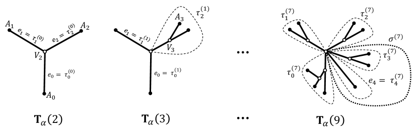
Figure 3: Illustration of Marchal’s random growth algorithm and notation employed

Denote the number of leaves in $\tau_{i}^{(n)}$ excluding $V_{2}$ by $N_{i}(n)$ for all $i=0,1,\ldots,K_{n}+2$, and define its inverse $N^{-1}_{i}(n):=\inf\{k\geq 0\colon N_{i}(k)=n\}$ as the first time $k$ at which $\tau_{i}^{(k)}$ has $n$ leaves excluding $V_{2}$, with the convention $\inf\emptyset=\infty$.

Regard $V_{2}$ as a (weightless) root from the perspective of each element of $\{\tau_{i}^{(n)},i=1,\ldots,K_{n}+2\}$ and as a marked leaf of $\tau_{0}^{(n)}$. For each $i=1,\ldots,K_{n}+2$, mark the first leaf created in $\tau_{i}^{(n)}$ by Marchal’s algorithm, that is, the other endpoint of $e_{i}$ which is not $V_{2}$. Recall that $A_{0}$ is the root of $\tau_{0}^{(n)}$.

In the limit, denote by $\tau_{i}^{(\infty)}$ the limiting set of vertices corresponding to the $i$-th subtree. Denote its associated $\mathbb{R}$-tree by $\tau_{i}$, obtained by the completion of $\tau_{i}^{(\infty)}$ in the scaling limit as described in Section 2.2. Likewise, define $\sigma^{(\infty)}$ and $\sigma$ as the limiting set of vertices and the $\mathbb{R}$-tree associated with $\sigma^{(n)}$, respectively.

Recall that $W(\cdot)$ measures the total weight of a given sub-structure, e.g., for each $i\in\{0,1,2\}$, $W(\tau_{i}^{(0)})=\alpha-1.$ The following result shows that the weight of a particular subtree only depends on the number of leaves it has, and not on its shape.

Lemma 3.1

Regardless of its shape, the total weight of the $i$-th subtree is $W(\tau^{(n)}_{i})\!=\!\alpha N_{i}(n)\!-\!1$ for $i=0,1,\ldots,K_{n}+2$ and $n\geq 0$.

• Proof. This follows simply by induction applied to each subtree. $\square$

Proposition 3.2

We have the following limiting results for weights.

1. For $\alpha=2$, $K_{n}=0$ a.s. for all $n\geq 0$. The relative weight split in $\mathbf{T}_{\alpha}(n)$ has an almost sure limit as $n\rightarrow\infty$ given by

   $$\left(\frac{W\left(\tau_{0}^{(n)}\right)}{2n+3},\frac{W\left(\tau_{1}^{(n)}\right)}{2n+3},\frac{W\left(\tau_{2}^{(n)}\right)}{2n+3}\right)\overset{a.s.}{\longrightarrow}\left(X_{0},X_{1},X_{2}\right)$$

   where $\left(X_{0},X_{1},X_{2}\right)\sim\textnormal{Dir}\left(1/2,1/2,1/2\right)$.

2. For $\alpha\in(1,2)$, $K_{n}\rightarrow\infty$ as $n\rightarrow\infty$ almost surely. The relative weight split in $\mathbf{T}_{\alpha}(n)$ has an almost sure limit as $n\rightarrow\infty$ given by

   $$\left(\!\frac{W\left(\tau_{0}^{(n)}\right)}{(n\!+\!2)\alpha\!-\!1},\frac{W\left(\tau_{1}^{(n)}\right)}{(n\!+\!2)\alpha\!-\!1},\frac{W\left(\tau_{2}^{(n)}\right)}{(n\!+\!2)\alpha\!-\!1},\frac{W\!\left(\sigma^{(n)}\right)\!+\!W\!\left(\{V_{2}\}\right)}{(n+2)\alpha-1}\!\right)\!\overset{a.s.}{\longrightarrow}\left(X_{0},X_{1},X_{2},X_{3}\right),$$ (11)

   where $\left(X_{0},X_{1},X_{2},X_{3}\right)\sim\textnormal{Dir}\left(\beta,\beta,\beta,1-2\beta\right)$. Within the last part, denote the eventual proportion of weight distributed to the subtree $\tau_{i+2}$ by $P_{i}$ for $i\geq 1$. Then,

   $$\left(P_{i},i\geq 1\right)\sim\textnormal{GEM}\left(1-\beta,1-2\beta\right).$$

   In particular, the subtrees $\tau_{i}$, $i\geq 3$, have a relative weights partition that follows a $\textnormal{PD}(1-\beta,1-2\beta)$ distribution, when ranked in decreasing order.

• Proof. We prove (ii). From Lemma 3.1, conditional on an edge or branch point in $\tau_{i}^{(n)}$ being selected in the next step of Marchal’s algorithm, we increase the weight in $\tau_{i}^{(n)}$ by $\alpha$. It is easy to check that this also holds for $\sigma^{(n)}$ with one weighted copy of $V_{2}$ included. Hence,

  $$\left(W\left(\tau_{0}^{(n)}\right),W\left(\tau_{1}^{(n)}\right),W\left(\tau_{2}^{(n)}\right),W\left(\sigma^{(n)}\right)+W\left(\{V_{2}\}\right)\right)$$ (12)

  evolves precisely as the Pólya urn scheme in Definition 2.11 with $K\!=\!4$, initialisation vector $\vec{\gamma}=\left(\alpha\!-\!1,\alpha\!-\!1,\alpha\!-\!1,2\!-\!\alpha\right)$ and step-size $t\!=\!\alpha$. Therefore, (11) holds by Proposition 2.12.

  Next, we focus on the subtrees within $\sigma^{(n)}$. The above implies that $W\left(\sigma^{(n)}\right)+W\left(\{V_{2}\}\right)\rightarrow\infty$ as $n\rightarrow\infty$ a.s.. So, a.s., we observe infinitely many leaves being added to $\left(\sigma^{(n)},n\geq 1\right)$. We may then condition on the times where a leaf is added to $\left(\sigma^{(n)},n\geq 1\right)$, say $(q_{i},i\geq 1)$, where $1\leq q_{1}<q_{2}<\cdots<q_{n}<q_{n+1}<\cdots$ is an infinite sequence a.s.. Conditional on the preceding event, the first leaf added creates $\tau_{3}^{(q_{1})}$. At each $r\in\{q_{n},\ldots,q_{n+1}-1\}$, we have $n$ leaves (not including $V_{2}$) with $K_{q_{n}}$ subtrees whose union is $\sigma^{(r)}$. For $j=3,\ldots,K_{q_{n}}+2$, $\tau^{(r)}_{j}$ has $N_{j}(q_{n})$ leaves (not including $V_{2}$), and so has total weight $\alpha N_{j}(q_{n})-1$, by Lemma 3.1. Thus, as the total weight of $V_{2}$ is $2+K_{q_{n}}-\alpha$, the total weight of $\sigma^{(r)}$ and $\{V_{2}\}$ is $\alpha n+(2-\alpha)$. At the next arrival time $q_{n+1}$, we add a leaf to $\tau^{(q_{n+1}-1)}_{j}$ with probability $\left(\alpha N_{j}(q_{n})-1\right)/\left(\alpha n+2-\alpha\right)$ and we create a new sub-tree with probability $\left(2+K_{q_{n}}-\alpha\right)/\left(\alpha n+2-\alpha\right)$. Regarding the leaves (excluding $V_{2}$) as customers and each subtree as a table, this models a Chinese restaurant process with parameters $(1-\beta,1-2\beta)$, according to Definition 2.13. From Proposition 2.14, $K_{n}\rightarrow\infty$ as $n\rightarrow\infty$ almost surely. Recall $q_{1}<\infty$ almost surely, so we may assume $n\geq q_{1}$. From Proposition 2.14, we can identify the almost sure limiting proportion of leaves split within subtrees of $\sigma$ as $\textnormal{GEM}(1-\beta,1-2\beta)$ holding along the increasing subsequence $(q_{i},i\geq 1)$. That is,

  $$\left(\frac{N_{3}(q_{n})}{n},\ldots,\frac{N_{K_{q_{n}}+2}(q_{n})}{n},0,0,\ldots\right)\overset{a.s.}{\longrightarrow}\left(P_{i},i\geq 1\right)\quad\text{ as }n\rightarrow\infty,$$

  where $\left(P_{i},i\geq 1\right)\sim\textnormal{GEM}(1-\beta,1-2\beta)$. Write $N_{\sigma}(n)$ as the number of leaves in $\sigma^{(n)}$ excluding $V_{2}$. Noting that $N_{\sigma}(n)>0$ for $n\geq q_{1}$, we may rephrase the above as

  $$\left(\frac{N_{3}(n)}{N_{\sigma}(n)},\ldots,\frac{N_{K_{n}+2}(n)}{N_{\sigma}(n)},0,0,\ldots\right)\overset{a.s.}{\longrightarrow}\left(P_{i},i\geq 1\right)\quad\text{ as }n\rightarrow\infty.$$ (13)

  Using the relation $W\left(\sigma^{(n)}\right)+W\left(\{V_{2}\}\right)=\alpha N_{\sigma}(n)+2-\alpha$, and the aggregation property of the Dirichlet distribution in Proposition 2.10 applied to (12), we get that

  $$\frac{N_{\sigma}(n)}{n}\overset{a.s.}{\longrightarrow}X_{3}\quad\text{ as }n\rightarrow\infty,$$ (14)

  where $X_{3}\sim\textnormal{Beta}(1-2\beta,3\beta)$. By the algebra of almost sure convergence,

  $$\left(\frac{N_{3}(n)}{n},\ldots,\frac{N_{K_{n}+2}(n)}{n},0,0,\ldots\right)\overset{a.s.}{\longrightarrow}\left(X_{3}P_{i},i\geq 1\right)\quad\text{ as }n\rightarrow\infty.$$

  Therefore, for all $j=3,\ldots,K_{n}+2$ and $n\geq q_{1}$, as we have $W\left(\tau^{(n)}_{j}\right)=\alpha N_{j}(n)-1$, the above implies that, jointly in $j$,

  $$\frac{W\left(\tau^{(n)}_{j}\right)}{(n+2)\alpha-1}=\frac{\frac{N_{j}(n)}{n}-\frac{1}{\alpha n}}{\frac{n+2}{n}-\frac{1}{\alpha n}}\overset{a.s.}{\longrightarrow}X_{3}P_{j-2}\quad\text{ as }n\rightarrow\infty,$$

  where $X_{3}\sim\textnormal{Beta}(1-2\beta,3\beta)$ and $(P_{i},i\geq 1)\sim\textnormal{GEM}(1-\beta,1-2\beta)$. Thus, we have obtained the almost sure limiting weight partition for the subtrees $(\tau_{j},j\geq 0)$. The proof of (i) follows noting that $\sigma^{(n)}=\emptyset$ for all $n\geq 1$ almost surely when $\alpha=2$. $\square$

We will establish the independence of $(X_{0},X_{1},X_{2},X_{3})$ and $(P_{i},i\geq 1)$ in Proposition 3.4 to fully specify the distribution of $(\xi_{j},j\geq 0)$.

3.2 Independent copies of Marchal’s algorithm at the first branch point

The proof of the following result is inspired by [20, Lemma 8] in considering transition times at which a leaf is added into a subtree. However, we extend the result from [20] by considering transitions jointly over multiple subtrees. We restrict our considerations to $\alpha\in(1,2)$, i.e. the infinitary case. The result can easily be extended to the Brownian case $\alpha=2$.

Proposition 3.3

For $n\geq 1$ and $i\geq 0$, we have $\tau_{i}^{(N^{-1}_{i}(n))}\overset{d}{=}\mathbf{T}(n)$. That is, at transition times in which a leaf is added into the $i$-th subtree, it evolves as Marchal’s algorithm with parameter $\alpha\in(1,2)$ with initial edge $e_{i}$. The sigma-field generated by

$$\left(\tau_{i}^{(N^{-1}_{i}(n))},n\geq 1\right)_{i\geq 0}$$

is independent of the sigma-field generated by $\left(N_{i}(n),n\!\geq\!1,i\!\geq\!0\right)$. Consequently, $\left(\tau_{i},i\!\geq\!0\right)$ are independent. Furthermore, $\left(\tau_{i},i\geq 0\right)$ is independent of $\left(N_{i}(n),n\geq 1,i\geq 0\right)$.

• Proof. From Proposition 3.2, we have $K_{n}\rightarrow\infty$ a.s. as $n\rightarrow\infty$. In particular, for all $i\geq 0$ and $n\geq 1$, $N^{-1}_{i}(n)<\infty$ a.s.. We assume this holds henceforth. It suffices to show the independence of the sigma-fields generated by

  $$\left(N_{i}(n),n\geq 1,i\geq 0\right)\qquad\text{and}\qquad\left(\tau_{i}^{(N^{-1}_{i}(n))},n\geq 1\right)_{0\leq i\leq m+2},$$

  respectively, where $m\geq 0$ is arbitrary but fixed.

  Consider a given time $n\geq N^{-1}_{m+2}(1)$. Conditional on a leaf being added to the $i$-th subtree for $0\leq i\leq m+2$, we have the dynamics of Marchal’s algorithm with parameter $\alpha$ by the weight-leaf relation in Lemma 3.1. Likewise, the transition in the other components, not including the $i$-th subtree for $0\leq i\leq m+2$, follows the correct conditional distributions of Marchal’s algorithm. This proves the distributional identity $\tau_{i}^{(N^{-1}_{i}(n))}\overset{d}{=}\mathbf{T}(n)$ at transition times in the $i$-th subtree for $0\leq i\leq m+2$.

  Let $M>1$ be arbitrary, but fixed, and denote the natural filtration of $\left(N_{i}(n),i\geq 0\right)_{n\geq 1}$ by $\left(\mathcal{F}_{n}\right)_{n\geq 1}$. Note that for any fixed $n\geq 1$, $\left(N_{i}(n),i\geq 0\right)$ is almost surely a vector with finitely many non-trivial entries. Define $T:=\max_{i=0,\ldots,m+2}N_{i}^{-1}(M)$, which is a stopping time with respect to $\left(\mathcal{F}_{n}\right)_{n\geq 1}$. By assumption, $T<\infty$ a.s.. Conditional on $\mathcal{F}_{T}$ (which is the same as conditioning on relative weights on subtrees until time $T$), we have factorisation of tree shape probabilities into tree shape probabilities for the respective subtrees cut at $V_{2}$. In particular, given $\mathcal{F}_{T}$, the tree shapes of

  $$\left(\tau_{i}^{(N^{-1}_{i}(n))},1\leq n\leq M\right)_{0\leq i\leq m+2}$$

  are independent. Furthermore, on the event $\{T=t\}$, conditioning on the sigma-field generated at a later time $k\geq t$ does not affect the tree shapes under consideration. Hence, the hypotheses in Lemma 2.16 are fulfilled. Let $\mathbf{t}_{i}^{(n)}$ be some given leaf-labelled trees with $n$ leaves and a root. Then,

  $$\mathbb{P}\left(\tau_{i}^{(N^{-1}_{i}(n))}=\mathbf{t}_{i}^{(n)},1\leq n\leq M,0\leq i\leq m+2~{}\bigg{\rvert}~{}\mathcal{F}_{\infty}\right)$$

  $$=\mathbb{P}\left(\tau_{i}^{(N^{-1}_{i}(n))}=\mathbf{t}_{i}^{(n)},1\leq n\leq M,0\leq i\leq m+2~{}\bigg{\rvert}~{}\mathcal{F}_{T}\right)$$

  $$=\mathbb{P}\left(\tau_{i}^{(N^{-1}_{i}(M))}=\mathbf{t}_{i}^{(M)},0\leq i\leq m+2~{}\bigg{\rvert}~{}\mathcal{F}_{T}\right)$$ (15)

  $$=\prod_{i=0}^{m+2}\mathbb{P}\left(\tau_{i}^{(N^{-1}_{i}(M))}=\mathbf{t}_{i}^{(M)}~{}\bigg{\rvert}~{}\mathcal{F}_{T}\right)$$ (16)

  $$=\prod_{i=0}^{m+2}\mathbb{P}\left(\mathbf{T}(M)=\mathbf{t}_{i}^{(M)}~{}\bigg{\rvert}~{}\mathcal{F}_{T}\right)$$ (17)

  $$=\prod_{i=0}^{m+2}\mathbb{P}\left(\mathbf{T}(M)=\mathbf{t}_{i}^{(M)}\right),$$ (18)

  where (15) holds since $\tau_{i}^{(N^{-1}_{i}(M))}$ determines $\tau_{i}^{(N^{-1}_{i}(n))}$ for all $1\leq n\leq M$, (16) holds by Proposition 2.6, and (18) follows since there is no dependence on $\mathcal{F}_{\infty}$ in evaluating (17) and we are conditioning over an almost surely finite number of discrete random variables. Furthermore, since the final expression does not depend on $\mathcal{F}_{\infty}$, the sigma-field of

  $$\left(\tau_{i}^{(N^{-1}_{i}(n))},1\leq n\leq M\right)_{0\leq i\leq m+2}$$

  is independent of $\mathcal{F}_{\infty}$. Letting $M\rightarrow\infty$, and recalling $m\geq 0$ is arbitrary, the claimed independence of the $\sigma$-fields follows.

  As the collection $(\tau_{i},i\geq 0)$ is measurably constructed from $(\tau_{i}^{(N^{-1}_{i}(n))},n\geq 1)_{i\geq 0},$ it is independent of $(N_{i}(n),n\geq 1,i\geq 0)$. Dropping the conditioning in (17), we get that $\big{(}\tau_{i}^{(N^{-1}_{i}(n))},1\leq n\leq M\big{)}$, $0\leq i\leq m+2$, are independent. Thus, in the limit as $M\rightarrow\infty$, $\big{(}\tau_{i}^{(N^{-1}_{i}(n))},n\geq 1\big{)}$, $0\leq i\leq m+2$, are independent. As $\tau_{i}$ is measurably constructed from $(\tau_{i}^{(N^{-1}_{i}(n))},n\geq 1)$ for each $0\leq i\leq m+2$, $\big{(}\tau_{i},0\leq i\leq m+2\big{)}$ are independent. Let $m\rightarrow\infty$ to conclude that $(\tau_{i},i\geq 0)$ are independent. $\square$

Proposition 3.4

For $\alpha\in(1,2)$, the random variables $\left(X_{0},X_{1},X_{2},X_{3}\right)$ and $\left(P_{i},i\geq 1\right)$ as defined in Proposition 3.2 are independent. In particular, this fully specifies their joint distribution.

• Proof. Recall that $N_{\sigma}(n)$ denotes the number of leaves (excluding $V_{2}$) in $\sigma^{(n)}$, and define $N_{\sigma}^{-1}(n):=\inf\{k\geq 0\colon N_{\sigma}(k)=n\}$. We claim that the sigma-field generated by $\left(N_{j}\left(N_{\sigma}^{-1}(n)\right),n\geq 1\right)_{j\geq 3}$ is independent of the sigma-field generated by

  $$\left(N_{0}^{-1}(n),N_{1}^{-1}(n),N_{2}^{-1}(n),N_{\sigma}^{-1}(n),n\geq 1\right).$$

  Let $(\mathcal{F}_{n})_{n\geq 1}$ denote the natural filtration of $(N_{0}^{-1}(n),N_{1}^{-1}(n),N_{2}^{-1}(n),N_{\sigma}^{-1}(n))_{n\geq 1}$. It suffices to prove that the sigma-field generated by $(N_{j}\left(N_{\sigma}^{-1}(n)),n\geq 1\right)_{3\leq j\leq m}$ is independent of $\mathcal{F}_{\infty}$, where $m\geq 3$ is arbitrary but fixed. By Proposition 3.2, almost surely, $N^{-1}_{\sigma}(n)<\infty$ for all $n\geq 1$. For $M\geq 1$ arbitrary but fixed, $T:=N^{-1}_{\sigma}(M)$ is an almost surely finite stopping time with respect to $(\mathcal{F}_{n})_{n\geq 1}$. Consider the random variables $(N_{j}(N_{\sigma}^{-1}(n)),1\leq n\leq M)_{3\leq j\leq m}$. On the event $\{T=t\}$, conditioning on the sigma-field generated at a later time $k\geq t$ does not affect conditional expectations. Hence, by Lemma 2.16, for all non-negative integers $l_{j}(n)$,

  $$\mathbb{P} \left(N_{j}\left(N_{\sigma}^{-1}(n)\right)=l_{j}(n),1\leq n\leq M,3\leq j\leq m~{}\bigg{\rvert}~{}\mathcal{F}_{\infty}\right)$$

  $$=\mathbb{P}\left(N_{j}\left(N_{\sigma}^{-1}(n)\right)=l_{j}(n),1\leq n\leq M,3\leq j\leq m~{}\bigg{\rvert}~{}\mathcal{F}_{T}\right)$$

  $$=\mathbb{P}\left(N_{j}\left(N_{\sigma}^{-1}(n)\right)=l_{j}(n),1\leq n\leq M,3\leq j\leq m\right).$$

  The last equality follows, since conditional on a leaf being added to $\sigma^{(n)}$ at time $n+1$, the process of adding leaves to each subtree within $\sigma^{(n)}$ is modelled by a CRP with parameters $(1-\beta,1-2\beta)$, see Proposition 3.2. Furthermore, it does not depend on the times at which the leaf is added. Since we are conditioning over an almost surely finite number of discrete random variables, we may drop conditioning on $\mathcal{F}_{T}$. This implies that the sigma-field generated by

  $$\left(N_{j}\left(N_{\sigma}^{-1}(n)\right),1\leq n\leq M\right)_{3\leq j\leq m}$$

  is independent of $\mathcal{F}_{\infty}$ for all $M\geq 1$. Let $M\rightarrow\infty$ to conclude that the sigma-field generated by $\left(N_{j}\left(N_{\sigma}^{-1}(n)\right),n\geq 1\right)_{3\leq j\leq m}$ is independent of $\mathcal{F}_{\infty}$, as desired. Since we may rewrite equation (14) to get

  $$\frac{n}{N^{-1}_{\sigma}(n)}\overset{a.s.}{\longrightarrow}X_{3}\quad\text{ as }n\rightarrow\infty,$$

  we conclude that $X_{3}$ is $\mathcal{F}_{\infty}$-measurable. Likewise, $X_{0},X_{1}$ and $X_{2}$ are $\mathcal{F}_{\infty}$-measurable. From (13),

  $$\frac{N_{i+2}\left(N_{\sigma}^{-1}(n)\right)}{n}\overset{a.s.}{\longrightarrow}P_{i}\quad\text{ as }n\rightarrow\infty,$$

  for all $i\geq 1$. So, $(P_{i},i\geq 1)$ is measurable with respect to the sigma-field generated by $\left(N_{j}\left(N_{\sigma}^{-1}(n)\right),n\geq 1\right)_{j\geq 3}$. The desired result follows. $\square$

We finally obtain the main result regarding the self-similarity of Marchal’s algorithm, which proves the self-similarity property of $\alpha$-stable trees when decomposed at the first branch point.

Theorem 3.5

For any $\alpha\in(1,2]$, the limiting trees $(\tau_{i},i\geq 0)$ in Marchal’s algorithm are independent. Furthermore, they are independent of their scaling factors. For each subtree $\tau_{i}^{(n)}$, let $d_{i}^{(n)}$ denote the graph distance and $\mu_{i}^{(n)}$ the empirical mass measure on its leaves.

1. If $\alpha=2$, for each $i\in\{0,1,2\}$, we have the convergence

   $$\left(\tau_{i}^{(n)},\frac{d_{i}^{(n)}}{2n^{1/2}},\mu_{i}^{(n)}\right)\overset{a.s.}{\longrightarrow}\left(\tau_{i},\xi_{i}^{1/2}d^{(\infty)}_{i},\xi_{i}\mu^{(\infty)}_{i}\right)\quad\text{ as }n\rightarrow\infty,$$

   in the Gromov–Hausdorff–Prokhorov topology, where $(\tau_{i},d^{(\infty)}_{i},\mu^{(\infty)}_{i}),i\geq 1$, are i.i.d. with

   $$\left(\tau_{i},d^{(\infty)}_{i},\mu^{(\infty)}_{i}\right)\,{\buildrel d\over{=}}\,\left(\mathcal{T}_{2},d_{2},\mu_{2}\right),\quad i=0,1,2,$$

   and $\left(\xi_{0},\xi_{1},\xi_{2}\right)\sim\textnormal{Dir}\left(1/2,1/2,1/2\right)$ is independent of $(\tau_{0},\tau_{1},\tau_{2})$.

2. If $\alpha\in(1,2)$, for each $i\geq 0$, we have the convergence

   $$\left(\tau_{i}^{(n)},\frac{d_{i}^{(n)}}{\alpha n^{\beta}},\mu_{i}^{(n)}\right)\overset{a.s.}{\longrightarrow}\left(\tau_{i},\xi_{i}^{\beta}d^{(\infty)}_{i},\xi_{i}\mu^{(\infty)}_{i}\right)\quad\text{ as }n\rightarrow\infty,$$

   in the Gromov–Hausdorff–Prokhorov topology, where $(\tau_{i},d^{(\infty)}_{i},\mu^{(\infty)}_{i}),i\geq 1,$ are i.i.d. with

   $$\left(\tau_{i},d^{(\infty)}_{i},\mu^{(\infty)}_{i}\right)\,{\buildrel d\over{=}}\,\left(\mathcal{T}_{\alpha},d_{\alpha},\mu_{\alpha}\right),\quad i\geq 0,$$

   and $\xi_{i}=X_{i}$ for $i\in\{0,1,2\}$ and $\xi_{j+2}=X_{3}P_{j}$ for $j\geq 1$, with $\left(X_{0},X_{1},X_{2},X_{3}\right)\sim\textnormal{Dir}\left(\beta,\beta,\beta,1-2\beta\right)$ and $(P_{i},i\geq 1)^{\downarrow}\sim\textnormal{PD}(1-\beta,1-2\beta)$ independent.

• Proof. The almost sure convergence in the rescaled subtrees arises by applying Proposition 2.8 and Proposition 3.2. The independence between the limiting subtrees comes immediately from Theorem 3.3. The arguments in Lemma 3.1 and Proposition 3.2 show that the limiting proportion of weights is measurably constructed from $(N_{i}(n),n\geq 1,i\geq 0)$. Hence, by Theorem 3.3, the limiting subtrees are independent of their scaling factors. The distribution of $(\xi_{i},i\geq 0)$ for $\alpha\in(1,2)$ is fully specified by Proposition 3.4. $\square$

The results of Theorem 3.5 agree with similar decompositions of the BCRT at a branch point in Aldous [8, Theorem 2], Albenque and Goldschmidt [4, Section 1.4], and Croydon and Hambly [18, Lemma 6], where the branch point is uniquely determined by a uniformly chosen point according to the mass measure within each of the three subtrees. We point out that Albenque and Goldschmidt deal with an unrooted BCRT, while Croydon and Hambly’s construction uses a doubly-marked rooted BCRT. Our construction thus far does not require a notion of a mass measure (even though we have chosen to include the mass measure in our statements), but rather a single marked point in each subtree.

3.3 Formal specification of the concatenation operation

After verifying that the subtrees $(\tau_{i},i\geq 0)$ are rescaled versions of $\mathcal{T}_{\alpha}$ in the limit with the required independences, the next step is to show that the concatenation operation induced by Marchal’s algorithm is well-defined and measurable as an operation on $\mathbb{T}_{\rm m}$. To this end, we adapt the general setup and terminology from [49]. Let

$$\Xi:=\bigg{\{}(x_{0},x_{1},x_{2},x_{3}p_{j},j\!\geq\!1)\colon x_{0},x_{1},x_{2},x_{3}\!\geq\!0,\,\sum_{i=0}^{3}x_{i}\!=\!1,\,p_{1}\!\geq\!p_{2}\!\geq\!\cdots\!\geq\!0,\,\sum_{j=1}^{\infty}p_{j}\!=\!1\bigg{\}}.\vspace{-0.2cm}$$

For notational convenience, we write $\xi_{i}=\left\{\begin{array}[]{ll}x_{i}&\text{if }i\in\{0,1,2\},\\ x_{3}p_{i-2}&\text{otherwise}.\end{array}\right.\vspace{0.1cm}$

Set $\Xi^{*}:=\Xi\times\mathbb{T}_{\rm m}^{\infty}$ as in (7) and recall that $\mathbb{T}_{\rm m}$ is the set of ${\rm GH}^{\rm m}$-equivalence classes of marked compact rooted $\mathbb{R}$-trees. Note that in our case, $N=\inf\{i\geq 0\colon\xi_{i+1}=0\}$ with the convention $\inf\emptyset=\infty$, so that $N$ is a function of $\xi=\left(\xi_{i},i\geq 0\right)\in\Xi$. Furthermore, in the case of $\alpha$-stable trees, recall that $N=2$ or $N=\infty$ almost surely. Hence, we drop dependence on $N$ in our notation. For $\beta\in\left(0,\frac{1}{2}\right]$, equip $\Xi^{*}$ with the metric

$$d_{\beta}\left(\left(\xi,\tau_{i},i\!\geq\!0\right),\left(\xi^{\prime},\tau^{\prime}_{i},i\!\geq\!0\right)\right):=\sup_{i\geq 0}\left(\lvert\xi_{i}^{\beta}\!-\!{\xi^{\prime}_{i}}^{\beta}\rvert\vee d_{\rm GH}^{\rm m}\left(\tau_{i},{\tau^{\prime}_{i}}\right)\vee d_{\rm GH}^{\rm m}\left(\xi_{i}^{\beta}\tau_{i},{\xi^{\prime}_{i}}^{\beta}{\tau^{\prime}_{i}}\right)\right),\vspace{-0.1cm}$$ (19)

where $\xi=\left(\xi_{i},i\geq 0\right)\in\Xi$, $\xi^{\prime}=\left(\xi_{i}^{\prime},i\geq 0\right)\in\Xi$, and $(\tau_{i},d_{i},\rho_{i},x_{i}),({\tau^{\prime}_{i}},d^{\prime},{\rho^{\prime}_{i}},{x^{\prime}_{i}})$ are representatives of ${\rm GH}^{\rm m}$-equivalence classes in $\mathbb{T}_{\rm m}$, with shorthand $\xi_{i}^{\beta}\tau_{i}$ meaning that all distances of $\tau_{i}$ are reduced by the factor $\xi_{i}^{\beta}$. However, as $d_{\rm GH}^{\rm m}$ only depends on ${\rm GH}^{\rm m}$-equivalence classes, our metric $d_{\beta}$ also only depends on ${\rm GH}^{\rm m}$-equivalence classes. Hence, we may define $d_{\beta}$ on $\Xi^{*}$ and denote by $\tau$ any representative of the ${\rm GH}^{\rm m}$-equivalence class of $(\tau,d,\rho,x)$.

Proposition 3.6

$\left(\Xi^{*},d_{\beta}\right)$ is a Polish metric space.

• Proof. This can be proved following the lines of the proof of [49, Proposition 3.1]. $\square$

We now formally define our concatenation operator. Let $\xi\in\Xi$ and let $\left(\tau_{i},d_{i},\rho_{i},x_{i}\right)$ be representatives of ${\rm GH}^{\rm m}$-equivalence classes in $\mathbb{T}_{\rm m}$ for $i\geq 0$. Define the concatenated tree $\left(\tau^{\prime},d^{\prime},\rho^{\prime},x^{\prime}\right)$ as follows.

1. Let $\widetilde{\tau}^{\prime}:=\coprod_{i\geq 0}\tau_{i}$ be the disjoint union of trees. Let $\sim_{c}$ be the equivalence relation on $\widetilde{\tau}^{\prime}$ in which $\rho_{i}\sim_{c}x_{0}$ for all $i\geq 1$. Define $\tau^{\prime}:=\widetilde{\tau}^{\prime}/\sim_{c}$. Write $\psi_{c}$ for the canonical projection from $\widetilde{\tau}^{\prime}$ onto $\tau^{\prime}$.

2. Define $d^{\prime}$ as the metric induced on $\tau^{\prime}$ under $\psi_{c}$ by the metric $\widetilde{d}^{\prime}$ on $\widetilde{\tau}^{\prime}$ such that

   $$\widetilde{d}^{\prime}(u,v)=\begin{cases}\xi^{\beta}_{i}d_{i}(u,v)&\text{if }u,v\in\tau_{i},i\geq 0,\\ \xi^{\beta}_{0}d_{0}(u,x_{0})+\xi^{\beta}_{j}d_{j}(\rho_{j},v)&\text{if }u\in\tau_{0}\text{ and }v\in\tau_{j},j\neq 0,\\ \xi^{\beta}_{i}d_{i}(u,\rho_{i})+\xi^{\beta}_{0}d_{0}(x_{0},v)&\text{if }u\in\tau_{i}\text{ and }v\in\tau_{0},i\neq 0,\\ \xi^{\beta}_{i}d_{i}(u,\rho_{i})+\xi^{\beta}_{j}d_{j}(\rho_{j},v)&\text{if }u\in\tau_{i}\text{ and }v\in\tau_{j},i,j\neq 0.\\ \end{cases}$$ (20)

3. Retain $x^{\prime}=\psi_{c}\left(x_{1}\right)$ as our marked point in $\tau^{\prime}$ and set $\rho^{\prime}=\psi_{c}\left(\rho_{0}\right)$ as the root of $\tau^{\prime}$.

We illustrate this construction in Figure 4.

   

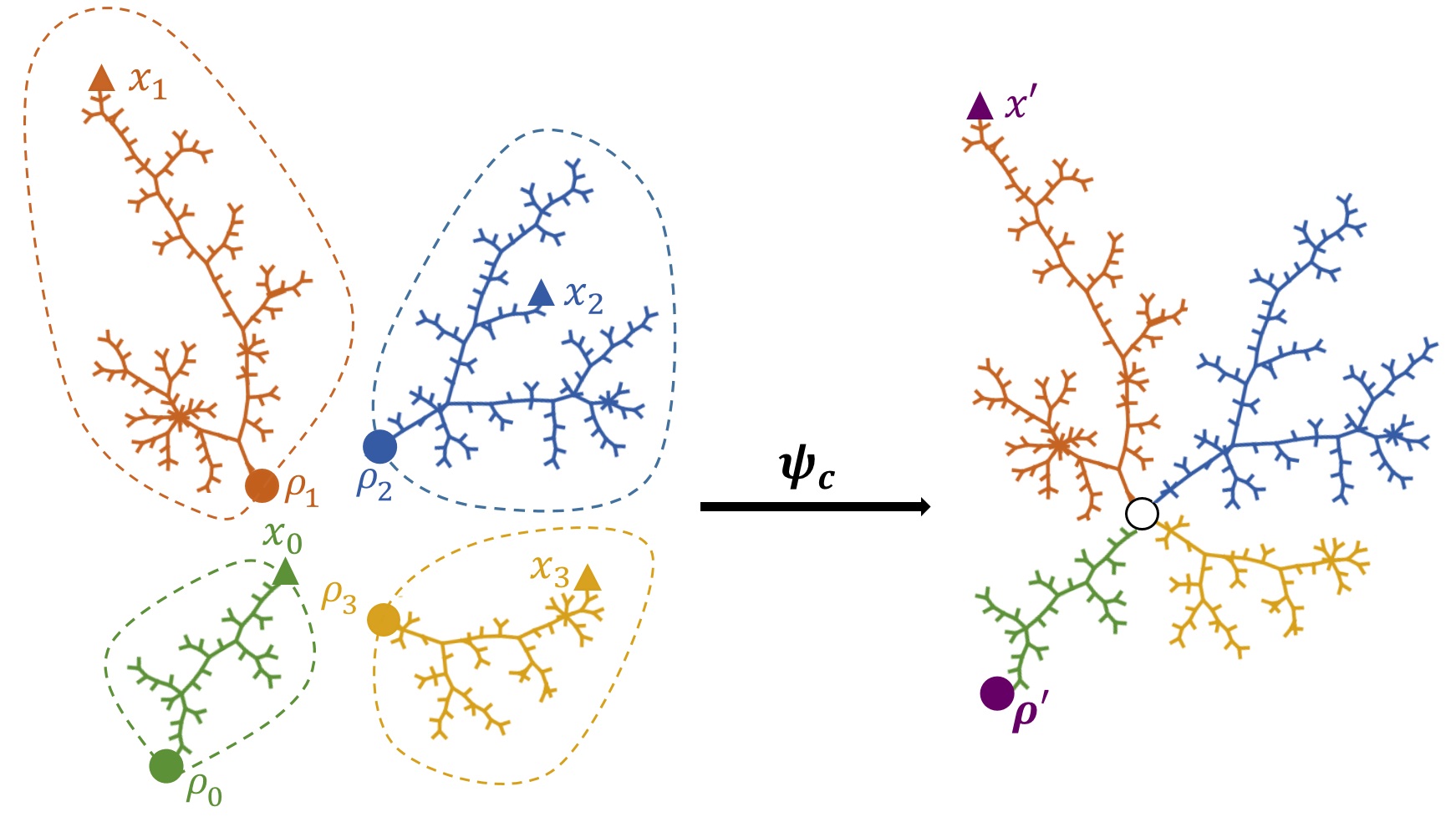
Figure 4: Construction of concatenated tree from 4 marked trees, rescaling is not shown; extracted from simulations (original simulations courtesy of Igor Kortchemski).

By virtue of this construction, the ${\rm GH}^{\rm m}$-equivalence class of $\left(\tau^{\prime},d^{\prime},\rho^{\prime},x^{\prime}\right)$ only depends on the ${\rm GH}^{\rm m}$-equivalence classes of $\left(\tau_{i},d_{i},\rho_{i},x_{i}\right)$ for $i\geq 0$. Thus, it makes sense to define $C_{\beta}\subseteq\Xi^{*}$ as the set of elements $\kappa=\left(\xi,\tau_{i},i\geq 0\right)\in\Xi^{*}$ such that the concatenated tree $\left(\tau^{\prime},d^{\prime},\rho^{\prime},x^{\prime}\right)$ formed by any equivalence class representatives of $\left(\left(\tau_{i},d_{i},\rho_{i},x_{i}\right),i\geq 0\right)$ is compact. Equip $\mathbb{T}_{\rm m}$ and $\Xi^{*}$ with their respective Borel sigma-algebras, $\mathcal{B}(\mathbb{T}_{\rm m})$ and $\mathcal{B}(\Xi^{*})$. The concatenation operator $g_{\beta}\colon\Xi^{*}\rightarrow\mathbb{T}_{\rm m}$ is,

$$g_{\beta}(\kappa)=\begin{cases}\left(\tau^{\prime},d^{\prime},\rho^{\prime},x^{\prime}\right)&\text{if }\kappa\in C_{\beta},\\ \left(\left\{x^{\prime}\right\},0,x^{\prime},x^{\prime}\right)&\text{otherwise},\end{cases}$$ (21)

where $(\{x^{\prime}\},0,x^{\prime},x^{\prime})$ denotes the equivalence class of a trivial one-point rooted tree.

Proposition 3.7

The map $g_{\beta}\colon\Xi^{*}\rightarrow\mathbb{T}_{\rm m}$ is $\mathcal{B}(\Xi^{*})$-measurable.

• Proof. The proof can be adapted from [49, Proposition 3.2]. $\square$

3.4 First main result: the RDE satisfied by the stable tree

We now deduce our main theorem in this section.

Theorem 3.8

The marked $\alpha$-stable tree $(\mathcal{T}_{\alpha},d_{\alpha},\mu_{\alpha},x_{\alpha})$ with $x_{\alpha}\sim\mu_{\alpha}$ satisfies the RDE

$$\mathcal{T}_{\alpha}\overset{d}{=}g_{\beta}\left(\xi,\mathcal{T}_{i},i\geq 0\right)$$ (22)

on $\mathbb{T}_{\rm m}$, where $(\mathcal{T}_{i},i\geq 0)$ is a sequence of independent copies of $\mathcal{T}_{\alpha}$, independent of $\xi=\left(X_{0},X_{1},X_{2},X_{3}P_{j},j\geq 1\right)\in\Xi$, and where the following holds.

• If $\alpha=2$, then $\xi_{j+2}=X_{3}P_{j}=0$ almost surely for all $j\geq 1$ and $\left(X_{0},X_{1},X_{2}\right)\sim\textnormal{Dir}\left(1/2,1/2,1/2\right)$.

• If $\alpha\in(1,2)$, then $\left(X_{0},X_{1},X_{2},X_{3}\right)\sim\textnormal{Dir}\left(\beta,\beta,\beta,1-2\beta\right)$ and $(P_{j},j\geq 1)\sim\textnormal{PD}(1-\beta,1-2\beta)$, where $\left(X_{0},X_{1},X_{2},X_{3}\right)$ and $(P_{j},j\geq 1)$ are independent.

In other words, the law of the marked $\alpha$-stable tree $\varsigma_{\alpha}^{\rm m}$ satisfies the fixpoint equation

$$\eta=\Phi_{\beta}\left(\eta\right)$$

on $\mathcal{P}(\mathbb{T}_{\rm m})$, where $\Phi_{\beta}\colon\mathcal{P}\left(\mathbb{T}_{\rm m}\right)\rightarrow\mathcal{P}\left(\mathbb{T}_{\rm m}\right)$ is the mapping on $\mathcal{P}(\mathbb{T}_{\rm m})$ induced by (22), and where we recall that $\mathcal{P}(\mathbb{T}_{\rm m})$ denotes the set of Borel probability measures on $\mathbb{T}_{\rm m}$.

• Proof. Recall that for the subtrees involved in the recursive application of Marchal’s algorithm, we regarded $V_{2}$ as a root and marked the first leaf in the $i$-th subtree for each $i\geq 1$. We regarded $A_{0}$ as the root for the overall tree, and $V_{2}$ as a marked leaf for the $0$-th subtree. Thus, our construction using Marchal’s algorithm agrees with the concatenation operator $g_{\beta}$ acting on the subtrees. Theorem 3.5 gives the required independences and the distribution of $\xi=\left(\xi_{i},i\geq 0\right)$. Proposition 3.7 ascertains the measurability of $g_{\beta}$. $\square$

In general, the marked $\alpha$-stable tree is not the only fixpoint of (22). Observe that if the metrics $d_{i}$ of (the representatives of) $\left(\tau_{i},d_{i},\rho_{i},x_{i}\right)\in\mathbb{T}_{\rm m}$ in (20) were multiplied by some constant $c>0$, then the concatenated tree will also have its metric $d^{\prime}$ multiplied by $c$. Furthermore, if the original concatenated tree were a marked compact rooted $\mathbb{R}$-tree, then so would the concatenated tree with metric multiplied by $c$. Thus, since $\left(\mathcal{T}_{\alpha},d_{\alpha},\rho_{\alpha},x_{\alpha}\right)$ is a distributional fixpoint of (22), so is $\left(\mathcal{T}_{\alpha},cd_{\alpha},\rho_{\alpha},x_{\alpha}\right)$ for any $c>0$.

Remark 3.9

There also exist solutions to RDE (22) with infinite $1/\beta$-th height moment. This can be shown by grafting mass-less length-$y$ branches onto a stable tree with intensity proportional to $y^{-1-1/\beta}dy\mu(dx)$, see e.g. [14] and [4] for such constructions in the context of related RDEs with finite concatenation operations – the arguments there are not affected by the change of setting here. We will establish uniqueness of the solution to (22) up to multiplication of distances by a constant, under suitable constraints on height moments.

4 Uniqueness and attraction for a general RDE on $\mathbb{T}_{\rm m}$

4.1 An RDE on $\mathbb{T}$ and associated constructions in $\mathbb{T}_{\rm w}$ of [49]

In [49], we established a recursive construction method for CRTs by successively replacing the atoms of a random string of beads, that is, a random interval $[0,L]$ for some $L>0$ equipped with a random discrete probability measure $\mu$, with scaled independent copies of itself. More general versions of the CRT construction using so-called generalised strings were established to capture multifurcating self-similar CRTs. We briefly recap our construction, and refer to [49] for more details.

Strings of beads can be represented in the form $([0,l],(x_{i})_{i\in I},(q_{i})_{i\in I})$ where $l>0$ denotes the length of the interval, and $x_{i}\in[0,l]$, $i\in I$, are distinct and describe the locations of the atoms with respective masses $q_{i}\geq 0,i\in I$, $\sum_{i\in I}q_{i}=1$, where $I$ is some countable index set. The concept of a string of beads can be generalised by allowing for non-distinct $x_{i}$’s. We call $\left([0,l],(x_{i})_{i\in I},(q_{i})_{i\in I}\right)$ a generalised string. The following theorem is a (slightly simplified) version of the main result in [49].

Theorem 4.1

Let $\beta\in(0,\infty)$ and $p>1/\beta$. Consider a random generalised string $\zeta=(\check{\mathcal{T}}_{0},(\check{X}^{(0)}_{i})_{i\in I},(\check{Q}^{(0)}_{i})_{i\in I})$ with length $L>0$ such that $\mathbb{E}[L^{p}]<\infty$, and atom masses $0\leq\check{Q}^{(0)}_{i}<1$ a.s. for all $i\in I$ and such that $\sum_{i\in I}\check{Q}^{(0)}_{i}=1$ a.s.. For $n\geq 0$, to obtain

$$\left(\check{\mathcal{T}}_{n+1},\left(\check{X}_{i}^{(n+1)}\right)_{i\in I},\left(\check{Q}^{(n+1)}_{i}\right)_{i\in I}\right)$$

conditionally given $(\check{\mathcal{T}}_{n},(\check{X}_{i}^{(n)})_{i\in I},(\check{Q}^{(n)}_{i})_{i\in I})$, attach to each $\check{X}_{i}^{(n)}\in\check{\mathcal{T}}_{n}$ an independent isometric copy of $\zeta$ with metric rescaled by $(\check{Q}^{(n)}_{i})^{\beta}$ and atom masses rescaled by $\check{Q}^{(n)}_{i}$.

Let $\check{\mu}_{n}=\sum_{i\in I}\check{Q}^{(n)}_{i}\delta_{\check{X_{i}}^{(n)}},n\geq 0.$ Then there exists a random weighted $\mathbb{R}$-tree $(\check{\mathcal{T}},\check{\mu})$ such that

$$\lim_{n\rightarrow\infty}\left(\check{\mathcal{T}}_{n},\check{\mu}_{n}\right)=\left(\check{\mathcal{T}},\check{\mu}\right)\qquad\text{a.s.}$$

in the Gromov–Hausdorff–Prokhorov topology in $\mathbb{T}_{\rm w}$. Furthermore, $\mathbb{E}[{\rm ht}(\check{\mathcal{T}})^{p}]<\infty$ for all $p<p^{*}:=\sup\{p\geq 1\colon\mathbb{E}[L^{p}]<\infty\}$.

The convergence in Theorem 4.1 holds in particular in the Gromov–Hausdorff sense when we omit mass measures. In fact, this construction is naturally carried out in the Banach space $\ell_{1}(\mathbb{U})$, $\mathbb{U}:=\bigcup_{n\geq 0}\mathbb{N}^{n}$, which is a variant of Aldous’s $\ell_{1}(\mathbb{N})$ since $\mathbb{U}$ is countable. So embedded, the convergence holds with respect to the Hausdorff metric (or a Hausdorff–Prokhorov metric) for compact subsets (equipped with a probability measure) of $\ell_{1}(\mathbb{U})$, as a consequence of the arguments of [49]. In particular, the $\alpha$-stable tree was characterised as the limit in the case of a $\beta$-generalised string for $\beta=1-1/\alpha\in(0,1/2]$, that is, a generalised string of the form

$$\left(\left[0,L\right],\left(X_{i}\right)_{i\geq 1},\left(P_{i}\right)_{i\geq 1}\right)$$

where, for $(Q_{m},m\geq 1)\sim{\rm PD}(\beta,\beta)$ independent of i.i.d. $(R_{j}^{(m)},j\geq 1)\sim{\rm PD}(1-\beta,-\beta)$, $m\geq 1$, the atom sizes are given via

$$\left(P_{i},i\geq 1\right)=\left(Q_{m}R_{j}^{(m)},j\geq 1,m\geq 1\right)^{\downarrow},$$

and the atom locations are defined via i.i.d. Unif$([0,1])$-variables $(U_{m},m\geq 1)$ and

$$L:=\lim_{m\rightarrow\infty}m\Gamma(1-\beta)Q_{m}^{\beta},\quad X_{i}=LU_{m}\text{ if }P_{i}=Q_{m}R_{j}^{(m)},\qquad i\geq 1.$$

4.2 Second main result: uniqueness and attraction for the new RDE

We now turn to the uniqueness and attraction of the fixpoints in (22). By Theorem 3.8 and Remark 3.9, uniqueness will only hold up to multiplication by a constant and under additional moment conditions on tree heights. As our setup works for more general $\xi\in\Xi$, we will broaden our scope, and consider the RDE (22) in a less specific setting.

It will be useful to work in the framework of a recursive tree process, as defined in Section 2.4. Let us consider a sequence of i.i.d. $\mathbb{R}$-trees with one marked leaf with distribution $\eta$ on $\mathbb{T}_{\rm m}$, and an i.i.d. family of sequences of scaling factors $(\xi_{\mathbf{u}i},i\geq 0),\mathbf{u}\in\mathbb{U},$ with some distribution $\nu$ on $\Xi$, where we recall the Ulam–Harris notation $\mathbb{U}=\bigcup_{n\geq 0}\mathbb{N}^{n}$.

For $n\geq 1$, we would like to study the distribution $\Phi_{\beta}^{n}(\eta)$ of $\mathcal{T}_{n}:=\tau^{(n)}_{\emptyset}$, where

$$\tau^{(n)}_{\mathbf{u}}:=g_{\beta}\left((\xi_{\mathbf{u}i},i\geq 0),\left(\tau^{(n)}_{\mathbf{u}i},i\geq 0\right)\right),\quad\mathbf{u}\in\mathbb{N}^{k},\quad k=n,\ldots,1,$$ (23)

for $\tau^{(n)}_{\mathbf{u}i}\sim\eta,i\geq 0$, $\mathbf{u}\in\mathbb{N}^{n}$, i.i.d.. Note that this setup induces a recursive tree process, and, in particular, a recursive tree framework $(((\xi_{\mathbf{u}i},i\geq 0),\mathbf{u}\in\mathbb{U}),g_{\beta})$.

Furthermore, let ${\mathcal{P}}_{\infty}(\mathbb{T}_{\rm m})\subset\mathcal{P}(\mathbb{T}_{\rm m})$ be defined as

$${\mathcal{P}}_{\infty}\left(\mathbb{T}_{\rm m}\right):=\left\{\eta\in\mathcal{P}\left(\mathbb{T}_{\rm m}\right)\colon\mathbb{E}\left[{\rm ht}\left(\mathcal{T}\right)^{p}\right]<\infty\text{ for all }p>0\text{ where }\left(\mathcal{T},d,\rho,x\right)\sim\eta\right\}.$$

Our main result in this section is as follows.

Theorem 4.2

For any $\Xi$-valued random variable $\xi\!=\!(\xi_{i},i\!\geq\!0)$ such that $\mathbb{P}(\xi_{0}\!+\!\xi_{1}\!<\!1)\!=\!1$ and $\mathbb{P}(\xi_{0}>0,\xi_{1}>0)=1$, choose $\beta\in(0,1)$ such that $\mathbb{E}[\xi_{0}^{\beta}+\xi_{1}^{\beta}]=1$. Then, for any $\eta\in\mathcal{P}_{\infty}(\mathbb{T}_{\rm m})$ with $h:=\mathbb{E}[d(\rho,x)]$ for $(\mathcal{T},d,\rho,x)\sim\eta$,

$$\Phi^{n}_{\beta}\left(\eta\right)\rightarrow\eta^{*}_{h}\text{ weakly as }n\rightarrow\infty,$$

where $\eta^{*}_{h}$ is the unique fixpoint of $\Phi_{\beta}$ in $\mathcal{P}_{\infty}(\mathbb{T}_{\rm m})$ with $\mathbb{E}[d^{*}(\rho^{*}\!,x^{*})]\!=\!h$ for $(\mathcal{T}^{*}\!,d^{*}\!,\rho^{*}\!,x^{*})\!\sim\!\eta^{*}_{h}$.

Note that the function $f\colon[0,1]\rightarrow(0,\infty)$, $\beta\mapsto\mathbb{E}[\xi_{0}^{\beta}+\xi_{1}^{\beta}]$ is continuous with $f(0)=2$ and $f(1)<1$ when $\mathbb{P}(\xi_{0}+\xi_{1}<1)=1$. Hence, there is always some $\beta\in(0,1)$ such that $f(\beta)=1$ in the situation of Theorem 4.2.

The uniqueness and attractiveness of the marked $\alpha$-stable tree in (22) is a direct consequence of Theorem 4.2.

Corollary 4.3

Let $\alpha\in(1,2]$ and set $\beta:=1-1/\alpha\in(0,1/2]$. Furthermore, let $\xi=(X_{0},X_{1},X_{2},X_{3}P_{j},j\geq 1)$ for independent $(X_{0},X_{1},X_{2},X_{3})\sim\rm{Dir}(\beta,\beta,\beta,1-2\beta)$ and $(P_{j},j\geq 1)\sim\rm{PD}(1-\beta,1-2\beta)$. Then the law $\varsigma_{\alpha}^{\rm m}$ of the marked $\alpha$-stable tree is the unique fixpoint of $\Phi_{\beta}$ on $\mathcal{P}_{\infty}(\mathbb{T}_{\rm m})$ with $\mathbb{E}[d(\rho,x)]=\alpha\Gamma(\beta)/\Gamma(2\beta)$ for $(\mathcal{T},d,\rho,x)\sim\eta$, $\eta\in\mathcal{P}_{\infty}(\mathbb{T}_{\rm m})$. Furthermore, for any $\eta\in\mathcal{P}_{\infty}(\mathbb{T}_{\rm m})$ with $\mathbb{E}[d(\rho,x)]=h$ for $(\mathcal{T},d,\rho,x)\sim\eta$, we have

$$\Phi_{\beta}^{n}\left(\eta\right)\rightarrow\varsigma^{\rm m}_{\alpha,h}\text{ weakly as }n\rightarrow\infty,$$

where $\varsigma^{\rm m}_{\alpha,h}$ denotes the distribution of the marked $\alpha$-stable tree with distances scaled by $h/(\alpha\Gamma(\beta)/\Gamma(2\beta))$.

• Proof. Apply Theorem 4.2 with the specific distribution for $\xi$, and $\beta=1-1/\alpha$. Furthermore, recall from Theorem 3.8 that the marked $\alpha$-stable tree is a fixpoint of the resulting RDE, is well-known to have height moments of all orders (e.g. from its construction via Theorem 4.1), and from Section 2.3 that the distance between the root and a uniformly sampled leaf of the $\alpha$-stable tree has distribution ${\rm ML}(\beta,\beta)$ scaled by $\alpha$, which has mean $\alpha\Gamma(\beta)/\Gamma(2\beta)$ by (6). $\square$

To prove Theorem 4.2, we first focus on the case when $\eta$ is supported on the space of probability measures on trivial trees, that is, single branch trees with a root and exactly one leaf (which is marked). We further require that the length of such a tree has moments of orders $p>0$. Specifically, we consider

$$\mathbb{T}_{\rm m}^{\rm tr}:=\left\{(\mathcal{T},d,0,y)\in\mathbb{T}_{\rm m}\colon\mathcal{T}=\llbracket 0,y\rrbracket,y>0\right\}.$$

For most of the proof, we will work in the special case of $\mathbb{T}_{\rm m}^{\rm tr}$-valued initial distributions:

Assumption (A): $\eta\!\in\!\mathcal{P}_{\infty}\!\left(\mathbb{T}_{\rm m}^{\textrm{tr}}\right)\!:=\!\left\{\eta\!\in\!\mathcal{P}\!\left(\mathbb{T}_{\rm m}^{\textrm{tr}}\right)\!\colon\mathbb{E}[({\rm ht}(\mathcal{T}))^{p}]\!<\!\infty\text{\,for\,all\,}p\!>\!0\text{\,where\,}\mathcal{T}\!\sim\!\eta\right\}$.

Under Assumption (A), we will show the convergence of the spine from the root to the marked point in the RDE (Section 4.3), the convergence of subtrees spanned by leaves up to recursion depth $k$ (Section 4.4), the CRT limit as $k\rightarrow\infty$ (Section 4.5) and establish that the RDE is attractive, pulling threads together via a tightness argument (Section 4.6). We finally strengthen this to lift Assumption (A) and complete the proof of Theorem 4.2.

For the remainder of this section, we write $(\mathcal{T}_{n},n\geq 0)$ for the sequence of trees constructed in (23) from $\tau^{(n)}_{\mathbf{u}j}\sim\eta,\mathbf{u}\in\mathbb{N}^{n},j\geq 0$. We write $Y_{\mathbf{u}j}:={\rm ht}(\tau^{(n)}_{\mathbf{u}j})$, $\mathbf{u}\in\mathbb{U}$, $j\geq 0$.

4.3 The spine from the root to the marked point in the RDE

We first study an $\mathcal{L}^{p}$-bounded martingale arising from the fixpoint equation in Theorem 4.2, which tracks the length of the spine from the root to the marked point.

Lemma 4.4

Let $\xi$ be a $\Xi$-valued random variable with $\mathbb{P}(\xi_{0}>0,\xi_{1}>0)=1$. Let $\beta\in(0,1]$ such that $\mathbb{E}[\xi_{0}^{\beta}+\xi_{1}^{\beta}]=1$, let $(\xi_{\mathbf{u}j},j\geq 0),\mathbf{u}\in\mathbb{U}$, be i.i.d. with the same distribution as $\xi$, and define

$$\overline{\xi}_{\mathbf{u}}:=\xi_{u_{1}}\xi_{u_{1}u_{2}}\cdots\xi_{u_{1}\ldots u_{n}},\quad\mathbf{u}=u_{1}\ldots u_{n}\in\mathbb{N}^{n},\quad n\geq 1.$$ (24)

Then the process

$$L_{n}=\sum_{\mathbf{u}\in\{0,1\}^{n}}\overline{\xi}_{\mathbf{u}}^{\beta}$$ (25)

is a mean-1 martingale that converges a.s. and in $\mathcal{L}^{p}$ for all $p\geq 1$.

• Proof. It is straightforward to show that $(L_{n},n\geq 0)$ is a martingale with $\mathbb{E}[L_{n}]=1$ for all $n\geq 1$. So we focus on the $\mathcal{L}^{p}$-boundedness. For $p=1$, we have for all $n\geq 1$,

  $$\mathbb{E}\left[L_{n}\right]=\sum_{\mathbf{u}\in\{0,1\}^{n}}\mathbb{E}\left[\xi_{u_{1}}^{\beta}\right]\cdots\mathbb{E}\left[\xi_{u_{1}\ldots u_{n}}^{\beta}\right]=\left(\mathbb{E}\left[\xi_{0}^{\beta}\right]+\mathbb{E}\left[\xi_{1}^{\beta}\right]\right)^{n}=1.$$

  Inductively, if for all $j\leq p-1$ and $n\geq 1$, we have $\mathbb{E}[L_{n}^{j}]\leq f(j)$, then for all $n\geq 1$,

  $$\mathbb{E}\left[L_{n}^{p}\right] =\sum_{\mathbf{u}^{(1)},\ldots,\mathbf{u}^{(p)}\in\{0,1\}^{n}}\mathbb{E}\left[\overline{\xi}_{\mathbf{u}^{(1)}}^{\beta}\cdots\overline{\xi}_{\mathbf{u}^{(p)}}^{\beta}\right]$$

  $$=\sum_{\mathbf{v}\in\{0,1\}^{n}}\mathbb{E}\left[\overline{\xi}_{\mathbf{v}}^{p\beta}\right]+\sum_{k=0}^{n-1}\sum_{\mathbf{v}\in\{0,1\}^{k}}\mathbb{E}\left[\overline{\xi}_{\mathbf{v}}^{p\beta}\right]\sum_{j=1}^{p-1}\binom{p}{j}\mathbb{E}\left[\xi_{0}^{j\beta}\xi_{1}^{(p-j)\beta}\right]$$

  $$\ \quad\qquad\qquad\qquad\times\mathbb{E}\!\left[\sum_{\begin{subarray}{c}\mathbf{w}^{(1)},\ldots,\mathbf{w}^{(j)}\\ \in\{0,1\}^{n-k-1}\end{subarray}}\!\!\!\left(\overline{\xi}_{\mathbf{w}^{(1)}}^{\beta}\cdots\overline{\xi}_{\mathbf{w}^{(j)}}^{\beta}\right)\!\right]!\!\mathbb{E}\!\left[\sum_{\begin{subarray}{c}\mathbf{w}^{(j+1)},\ldots,\mathbf{w}^{(p)}\\ \in\{0,1\}^{n-k-1}\end{subarray}}\!\!\!\left(\overline{\xi}_{\mathbf{w}^{(j+1)}}^{\beta}\cdots\overline{\xi}_{\mathbf{w}^{(p)}}^{\beta}\right)\!\right].$$

  Specifically, we split the sum over $\mathbf{u}^{(1)},\ldots,\mathbf{u}^{(p)}$ according to the number $k$ of initial entries that are common to all $\mathbf{u}^{(1)},\ldots,\mathbf{u}^{(p)}$ and according to the number $j$ of entries in the $(k+1)$-st place of $\mathbf{u}^{(1)},\ldots,\mathbf{u}^{(p)}$ that equal 0. For each $k$ and $j$, there are $\binom{p}{j}$ ways to choose which $j$ they are. By symmetry, the contribution is the same as if they are $1,\ldots,j$, so that we write the sum as a sum over

  $$\mathbf{u}^{(1)}=\mathbf{v}0\mathbf{w}^{(1)},\ldots,\mathbf{u}^{(j)}=\mathbf{v}0\mathbf{w}^{(j)},\mathbf{u}^{(j+1)}=\mathbf{v}1\mathbf{w}^{(j+1)},\ldots,\mathbf{u}^{(p)}=\mathbf{v}1\mathbf{w}^{(p)}.$$

  By the induction hypothesis, we can further bound $\mathbb{E}[L_{n}^{p}]$ above by

  $$\sum_{k=0}^{n}\sum_{\mathbf{v}\in\{0,1\}^{k}}\mathbb{E}\left[\overline{\xi}_{\mathbf{v}}^{p\beta}\right]\sum_{j=1}^{p-1}\binom{p}{j}f(j)f(p-j)$$

  $$\leq\left(\sum_{j=1}^{p-1}\binom{p}{j}f(j)f(p-j)\right)\frac{1}{1-\mathbb{E}\left[\xi_{0}^{p\beta}+\xi_{1}^{p\beta}\right]}=:f(p)<\infty.$$

  This completes the proof by the Martingale Convergence Theorem. $\square$

4.4 Convergence of subtrees spanned by leaves up to depth $k$

For the following, it will be useful to represent the trees $\mathcal{T}_{n}:=\tau_{\emptyset}^{(n)}$ of (23) in such a way that we can talk about “the subtree of $\mathcal{T}_{n}$ spanned by the leaves up to depth $k$”. Let us introduce notation for these leaves under the Assumption (A): denote by $\Sigma_{n,\mathbf{u}}$ the endpoint of the trivial tree $\tau_{\mathbf{u}}^{(n)}$ when repeatedly rescaled and finally used to build $\mathcal{T}_{n}$. Then the leaves of $\mathcal{T}_{n}$ up to depth $k$, together with the branch points up to depth $k$, are given by the set of $\Sigma_{n,\mathbf{u}}$ for $\mathbf{u}=u_{1}\cdots u_{n}\in\mathbb{N}^{n}$, with $u_{k+1}=\ldots=u_{n}=1$.

Proposition 4.5

Suppose Assumption (A) holds and $\mathcal{T}_{n}:=\tau_{\emptyset}^{(n)}$ in the setting of (23), $n\geq 0$. Let $k\in\mathbb{N}$. For $n\geq k$, let $\mathcal{T}_{n}^{k}$ be the subtree of $\mathcal{T}_{n}$ spanned by the root and the leaves up to depth $k$. We consider $\Sigma_{n,11\cdots 1}$ as the respective marked point. Then there is an increasing sequence of marked trees $(\mathcal{T}^{k},k\geq 0)$ such that, for all $k\geq 0$,

$$\mathcal{T}_{n}^{k}\rightarrow\mathcal{T}^{k}\text{ in probability as }n\rightarrow\infty$$

in the marked Gromov–Hausdorff topology.

• Proof. For $k=0$, $\mathcal{T}_{n}^{0}$ is a trivial one-branch tree with a root and a marked leaf, and total length

  $$\widetilde{L}_{n}^{0}=\sum_{\mathbf{u}\in\{0,1\}^{n}}\overline{\xi}_{\mathbf{u}}^{\beta}Y_{\mathbf{u}}.$$

  Recall the martingale $(L_{n},n\geq 1)$ from (25) and denote its limit by $L_{\infty}$. Let $m:=\mathbb{E}[Y_{\emptyset}]$, and note that,

  $$\mathbb{E}\left[\left(\widetilde{L}^{0}_{n}-mL_{n}\right)^{2}\right] =\mathbb{E}\left[\left(\sum_{\mathbf{u}\in\{0,1\}^{n}}\overline{\xi}_{\mathbf{u}}^{\beta}\left(Y_{\mathbf{u}}-m\right)\right)^{2}\right]$$

  $$=\sum_{\mathbf{u}\in\{0,1\}^{n}}\sum_{\mathbf{v}\in\{0,1\}^{n}}\mathbb{E}\left[\overline{\xi}_{\mathbf{u}}^{\beta}\overline{\xi}_{\mathbf{v}}^{\beta}\right]\mathbb{E}\left[\left(Y_{\mathbf{u}}-m\right)\left(Y_{\mathbf{v}}-m\right)\right]$$

  $$=\sum_{\mathbf{u}\in\{0,1\}^{n}}\mathbb{E}\left[\overline{\xi}_{\mathbf{u}}^{2\beta}\right]\mathbb{E}\left[\left(Y_{\mathbf{u}}-m\right)^{2}\right]={\rm Var}\left(Y\right)\left(\mathbb{E}\left[\xi_{0}^{2\beta}+\xi_{1}^{2\beta}\right]\right)^{n}\rightarrow 0$$

  as $n\rightarrow\infty$, where we used the facts that $Y_{\mathbf{u}}$ and $Y_{\mathbf{v}}$ are independent for $\mathbf{u}\neq\mathbf{v}$, and $\mathbb{E}[\xi_{0}^{2\beta}+\xi_{1}^{2\beta}]<1$ as $0<\xi_{0},\xi_{1}<1$ a.s.. Therefore, $\widetilde{L}_{n}^{0}\rightarrow\widetilde{L}^{0}_{\infty}:=m\cdot L_{\infty}$ in $\mathcal{L}^{2}$ and almost surely as $n\rightarrow\infty$.

  Under Assumption (A), the $Y_{\mathbf{u}}$ also have finite $p$-th moment for all $p\geq 3$ and splitting $p$-fold sums as in the proof of Lemma 4.4, it is straightforward to strengthen this convergence to $\mathcal{L}^{p}$-convergence.

  Now, let $k\geq 1$, and note that the shapes of $\mathcal{T}_{n}^{k}$ and $\mathcal{T}_{k}$ coincide for all $n\geq k$. Let $\widetilde{L}^{k}_{n,\mathbf{u}},\mathbf{u}\in\mathbb{N}^{k}$, denote the lengths of the edges of $\mathcal{T}_{n}^{k}$ using obvious notation, i.e.

  $$\widetilde{L}^{k}_{n,\mathbf{u}}:=\sum_{\mathbf{v}\in\{0,1\}^{n-k}}\overline{\xi}_{\mathbf{u}\mathbf{v}}^{\beta}Y_{\mathbf{u}\mathbf{v}},\quad\mathbf{u}\in\mathbb{N}^{k}.$$

  Furthermore, let $\mathcal{T}^{k}$ have the same shape and the same marked leaf as $\mathcal{T}_{k}$ with edge lengths $\widetilde{L}^{k}_{\infty,\mathbf{u}},\mathbf{u}\in\mathbb{N}^{k}$, given by

  $$\widetilde{L}^{k}_{\infty,\mathbf{u}}=\lim_{t\rightarrow\infty}\sum_{\mathbf{v}\in\{0,1\}^{t}}\overline{\xi}_{\mathbf{u}\mathbf{v}}^{\beta}Y_{\mathbf{u}\mathbf{v}},\quad\mathbf{u}\in\mathbb{N}^{k},$$

  which exists a.s. as a $\overline{\xi}_{\mathbf{u}}^{\beta}$-scaled copy of $\widetilde{L}^{0}_{\infty}$, independent for $\mathbf{u}\in\mathbb{N}^{k}$.

Hence, for each $k\geq 0$, the differences $\left\lvert{\widetilde{L}_{n,\mathbf{u}}^{k}-\widetilde{L}^{k}_{\infty,\mathbf{u}}}\right\rvert$, $\mathbf{u}\in\mathbb{N}^{k}$, are $\overline{\xi}_{\mathbf{u}}^{\beta}$-scaled independent copies of $\lvert\widetilde{L}_{n}^{0}-\widetilde{L}^{0}_{\infty}\rvert$. Therefore, for $p\geq 1/\beta$, as every leaf of $\mathcal{T}_{n}^{k}$ or $\mathcal{T}^{k}$ is at most $2^{k}$ edges from the root and from another leaf, by (4),

$$\mathbb{E}\left[\left(d^{\rm m}_{\rm GH}\left(\mathcal{T}_{n}^{k},\mathcal{T}^{k}\right)\right)^{p}\right]\leq 2^{pk}\mathbb{E}\left[\max_{\mathbf{u}\in\mathbb{N}^{k}}\left\lvert\widetilde{L}_{n,\mathbf{u}}^{k}-\widetilde{L}^{k}_{\infty,\mathbf{u}}\right\rvert^{p}\right] \leq 2^{pk}\sum_{\mathbf{u}\in\mathbb{N}^{k}}\mathbb{E}\left[\left(\left\lvert\widetilde{L}_{n,\mathbf{u}}^{k}-\widetilde{L}^{k}_{\infty,\mathbf{u}}\right\rvert\right)^{p}\right]$$

$$=2^{pk}\sum_{\mathbf{u}\in\mathbb{N}^{k}}\mathbb{E}\left[\overline{\xi}_{\mathbf{u}}^{p\beta}\right]\mathbb{E}\left[\left\lvert\widetilde{L}_{n}^{0}-\widetilde{L}^{0}_{\infty}\right\rvert^{p}\right].$$

Since $\sum_{\mathbf{u}\in\mathbb{N}^{k}}\mathbb{E}\left[\overline{\xi}_{\mathbf{u}}^{p\beta}\right]<\infty$ for $p\geq 1/\beta$ and $\widetilde{L}_{n}^{0}\rightarrow\widetilde{L}^{0}_{\infty}$ in $\mathcal{L}^{p}$ as $n\rightarrow\infty$, we conclude that, for any $\epsilon>0$,

$$\lim_{n\rightarrow\infty}\mathbb{P}\left(d^{\rm m}_{\rm GH}\left(\mathcal{T}_{n}^{k},\mathcal{T}^{k}\right)>\epsilon\right)\leq\lim_{n\rightarrow\infty}\epsilon^{-p}\mathbb{E}\left[\left(d^{\rm m}_{\rm GH}\left(\mathcal{T}_{n}^{k},\mathcal{T}^{k}\right)\right)^{p}\right]=0.$$

Hence, $\mathcal{T}_{n}^{k}\rightarrow\mathcal{T}^{k}$ in probability in the marked Gromov–Hausdorff topology as $n\rightarrow\infty$. $\square$

4.5 The CRT limit of $\mathcal{T}^{k}$ as $k\rightarrow\infty$

Next, we want to prove the convergence of $\mathcal{T}^{k}$ as $k\rightarrow\infty$. To this end, we need to identify a suitable candidate for the limit. We employ the recursive construction method for CRTs as described in Section 4.1. Define a generalised string

$$\zeta=\left(\left[0,\widetilde{L}^{0}_{\infty}\right],\left(X_{\mathbf{u}}\right)_{\mathbf{u}\in\mathbb{U}^{*}},\left(Q_{\mathbf{u}}\right)_{\mathbf{u}\in\mathbb{U}^{*}}\right)$$ (26)

where $\mathbb{U}^{*}:=\bigcup_{n\geq 0}\{0,1\}^{n}\times\{2,3,\ldots\}$, $\widetilde{L}^{0}_{\infty}$ is given above, and $(X_{\mathbf{u}})_{\mathbf{u}\in\mathbb{U}^{*}},(Q_{\mathbf{u}})_{\mathbf{u}\in\mathbb{U}^{*}}$ are defined by dyadically splitting $\widetilde{L}^{0}$ as follows. See Figure 5 for an illustration.

• Let $Q_{i}:=\xi_{i}$, $i\geq 2$, and, for $\mathbf{u}=u_{1}\ldots u_{n}\in\mathbb{U}^{*}$, define

  $$Q_{\mathbf{u}}:=\xi_{u_{1}}\xi_{u_{1}u_{2}}\cdots\xi_{u_{1}u_{2}\ldots u_{n}}=\overline{\xi}_{u_{1}u_{2}\ldots u_{n}}.$$

  Note that $0\leq Q_{\mathbf{u}}<1$ a.s. for all $\mathbf{u}\in\mathbb{U}^{*}$, $\sum_{\mathbf{u}\in\mathbb{U}^{*}}Q_{\mathbf{u}}=1$ a.s., and $\mathbb{E}\left[\sum_{\mathbf{u}\in\mathbb{U}^{*}}Q_{\mathbf{u}}^{p\beta}\right]<1$ for all $p>1/\beta$.

• Define the locations $\left(X_{\mathbf{u}}\right)_{\mathbf{u}\in\mathbb{U}^{*}}$ of the atoms with respective masses $\left(Q_{\mathbf{u}}\right)_{\mathbf{u}\in\mathbb{U}^{*}}$ by

  $$X_{i}=\lim_{m\rightarrow\infty}\sum_{(0u_{2}\ldots u_{m})\in\{0\}\times\{0,1\}^{m-1}}\overline{\xi}_{0u_{2}\ldots u_{m}}^{\beta}Y_{0u_{2}\ldots u_{m}},\quad i\geq 2,$$

  and, for general $\mathbf{u}=(u_{1}\ldots u_{n})\in\mathbb{U}^{*}$,

  $$X_{u_{1}\ldots u_{n}}\!=\!\lim_{m\rightarrow\infty}\!\left\{\!\sum_{\begin{subarray}{c}(v_{1}\ldots v_{n})\in\{0,1\}^{n}\colon(v_{1}\ldots v_{n})\prec(u_{1}\ldots u_{n})\\ (v_{1},\ldots,v_{n-1},v_{n})\neq(u_{1},\ldots,u_{n-1},1)\end{subarray}}\ \sum_{v_{n+1}\ldots v_{n+m}\in\{0,1\}^{m}}\!\overline{\xi}_{v_{1}\ldots v_{n+m}}^{\beta}Y_{v_{1}\ldots v_{n+m}}\!\right\}$$

  where $\prec$ denotes the lexicographic order, that is,

  $$(v_{1}\ldots v_{n})\prec(u_{1}\ldots u_{n})\iff\exists t\geq 1\text{ such that }\forall k<t\colon v_{k}=u_{k}\text{ and }v_{t}<u_{t}.$$

Noting in particular that this specifies $X_{\mathbf{u}i}=X_{\mathbf{u}2}$ for all $i\geq 2$ and each $\mathbf{u}2\in\mathbb{U}^{*}$, the scaled lengths and dyadic splits to depth $k=3$ are illustrated in Figure 5.

Figure 5: Dyadic structure of limiting branch lengths $\widetilde{L}_{\infty,\mathbf{u}}^{k}=\widetilde{L}_{\infty,\mathbf{u}0}^{k+1}+\widetilde{L}_{\infty,\mathbf{u}1}^{k+1}$, for which $\overline{\xi}_{\mathbf{u}}^{-\beta}\widetilde{L}_{\infty,\mathbf{u}}^{k}$, $\mathbf{u}\in\{0,1\}^{k}$ are i.i.d. for each $k\geq 1$, ordered in lexicographical order; atom positions $X_{\mathbf{u}i}$ are between fragments $\widetilde{L}_{\infty,\mathbf{u}0}^{n}$ and $\widetilde{L}_{\infty,\mathbf{u}1}^{n}$, $\mathbf{u}\in\{0,1\}^{n}$, $n\geq 0$.

We now apply the recursive construction as outlined in Theorem 4.1 to the generalised string $\zeta$, which results in an $\mathbb{R}$-tree $\mathcal{T}$, whose distribution we denote by $\eta^{*}$.

Proposition 4.6

Let $\beta\in(0,1]$, and $p>1/\beta$. Consider the generalised string $\zeta$ given by (26). Apply the recursive construction described in Theorem 4.1 to construct a sequence of random $\mathbb{R}$-trees $(\mathcal{T}_{n}^{*},n\geq 0)$. Then $\mathcal{T}_{n}^{*}\rightarrow\mathcal{T}$ a.s. in the Gromov–Hausdorff topology for some random compact $\mathbb{R}$-tree $\mathcal{T}$ with

$$\mathbb{E}\left[{\rm ht}\left(\mathcal{T}\right)^{p}\right]<\infty\text{ for all }p>0.$$

• Proof. This is a direct application of Theorem 4.1. $\square$

It will be convenient to refer to the root as $\rho$ and the endpoints of the generalised strings as $\Sigma_{\mathbf{u}}$, $\mathbf{u}\in\mathbb{U}$. Specifically, we denote by $\Sigma_{\emptyset}$ the endpoint of $\mathcal{T}_{0}^{*}$. In the first step of the construction performed in Proposition 4.6, we attach branches to all branch points on the initial spine at once. The string has all the branch points $X_{\mathbf{u}}$, $\mathbf{u}\in\mathbb{U}^{*}=\bigcup_{j\geq 0}\{0,1\}^{j}\times\{2,3,\ldots\}$ placed as in the $n\rightarrow\infty$ limit. In particular, we have $\Sigma_{\mathbf{u}}\in\mathcal{T}_{1}^{*}$ for all $\mathbf{u}\in\mathbb{U}^{*}$ and for more general $\mathbf{u}\in\mathbb{U}$, we have $\Sigma_{\mathbf{u}}\in\mathcal{T}_{n}^{*}$ if and only if $\mathbf{u}=u_{1}\cdots u_{j}$ has at most $n$ entries $u_{i}\in\{2,3,\ldots\}$, i.e. at least $j-n$ entries $u_{i}\in\{0,1\}$.

In contrast, as $(\mathcal{T}_{n},n\geq 0)$ evolves, the branch points on the initial spine are created successively, and distances change in each step as branches are replaced by two scaled branches in each step. We will further couple the vectors $(\xi_{\mathbf{u}i},i\geq 0)$, $\mathbf{u}\in\mathbb{U}$, of the construction of $(\mathcal{T}_{n},n\geq 0)$, and the generalised strings $\zeta_{\mathbf{v}}$, $\mathbf{v}\in\mathbb{U}$. Specifically, we take $\widetilde{L}^{k}_{\infty,\mathbf{v}}$ as the length of $\zeta_{\mathbf{v}}$ and build $((X_{\mathbf{v},\mathbf{u}})_{\mathbf{u}\in\mathbb{U}^{*}},(Q_{\mathbf{v},\mathbf{u}})_{\mathbf{u}\in\mathbb{U}^{*}})$ from the appropriate subfamilies of $((\xi_{\mathbf{u}i},i\geq 0),\mathbf{u}\in\mathbb{U})$. We will not require precise notation for these subfamilies, but we will exploit the coupling and the independence of these subfamilies for all $\mathbf{v}\in\mathbb{N}^{n}$, $n\geq 0$, which is a consequence of the branching property of the recursive tree framework $((\xi_{\mathbf{u}i},i\geq 0),\mathbf{u}\in\mathbb{U})$.

Indeed, we can represent $\mathcal{T}$ like $\mathcal{T}_{n}$, $n\geq 0$, in $\ell_{1}(\mathbb{U})$ in such a way that the convergence of Proposition 4.5 holds for the Hausdorff metric on compact subsets of $\ell_{1}(\mathbb{U})$. Then, we have further a.s. convergence of $\Sigma_{n,\mathbf{u}}$ to limits that we denote by $\Sigma_{\mathbf{u}}$, for all $\mathbf{u}\in\mathbb{U}$. Then the trees $\mathcal{T}^{k}$ are spanned by $\Sigma_{\mathbf{u}}$, $\mathbf{u}\in\bigcup_{0\leq j\leq k}\mathbb{N}^{j}$, while $\mathcal{T}_{n}^{*}$ is spanned by $\Sigma_{\mathbf{u}}$, $\mathbf{u}=\mathbf{u}^{(1)}v_{1}\mathbf{u}^{(2)}v_{2}\cdots\mathbf{u}^{(n)}v_{n}\mathbf{u}^{(n+1)}$, $\mathbf{u}^{(1)},\ldots,\mathbf{u}^{(n+1)}\in\bigcup_{m\geq 0}\{0,1\}^{m}$, $v_{1},\ldots,v_{n}\in\mathbb{N}$.

Lemma 4.7

Let $(\mathcal{T}^{k},k\geq 0)$ be the sequence of trees from Proposition 4.5, and let $(\mathcal{T}_{n}^{*},n\geq 0)$ be the sequence of trees from Proposition 4.6 with $\mathcal{T}_{n}^{*}\rightarrow\mathcal{T}$ a.s. as $n\rightarrow\infty$. Then

$$\mathcal{T}^{k}\rightarrow\mathcal{T}\text{ a.s. as }k\rightarrow\infty$$

in the marked Gromov–Hausdorff topology.

• Proof. Since the sequence of trees $(\mathcal{T}^{k},k\geq 0)$ is increasing and embedded in $\mathcal{T}$ with the same marked point, it remains to show that the almost sure limit of $\mathcal{T}^{k}$ is the whole of $\mathcal{T}$.

  Let $(\mathcal{T}_{\mathbf{u}j},j\geq 2)$, $\mathbf{u}\in\bigcup_{t=0}^{\infty}\mathbb{N}^{k}\times\{0,1\}^{t}$, denote the connected components of $\mathcal{T}\setminus\mathcal{T}^{k}$, $k\geq 0$, where we write $(\mathcal{T}_{{u_{1}\ldots u_{n}}j},j\geq 2)$ for the subtrees of $\mathcal{T}\setminus\mathcal{T}^{k}$ rooted at the edge of $\mathcal{T}_{k}$ of length $\widetilde{L}_{\infty,{u_{1}\ldots u_{k}}}^{k}$, $n\geq k$, using notation from Proposition 4.5. Exploiting the fact that each $\mathcal{T}_{\mathbf{u}j}$ is a $\overline{\xi}_{\mathbf{u}j}$ scaled independent copy of $\mathcal{T}$, we obtain for $k\geq 0$ and $p>1/\beta$,

  $$\mathbb{E}\left[\left(d_{\rm GH}^{\rm m}\left(\mathcal{T}^{k},\mathcal{T}\right)\right)^{p}\right] \leq\mathbb{E}\left[\left(\max_{\mathbf{u}\in\bigcup_{t=0}^{\infty}\mathbb{N}^{k}\times\{0,1\}^{t},j\geq 2}{\rm ht}\left(\mathcal{T}_{\mathbf{u}j}\right)\right)^{p}\right]$$

  $$\leq\mathbb{E}\left[\left({\rm ht}\left(\mathcal{T}\right)\right)^{p}\right]\sum_{\mathbf{u}\in\bigcup_{t=0}^{\infty}\mathbb{N}^{k}\times\{0,1\}^{t},j\geq 2}\mathbb{E}\left[\overline{\xi}_{\mathbf{u}j}^{p\beta}\right]$$

  $$\leq\mathbb{E}\left[\left({\rm ht}\left(\mathcal{T}\right)\right)^{p}\right]\sum_{\mathbf{u}\in\bigcup_{t=0}^{\infty}\mathbb{N}^{k}\times\{0,1\}^{t}}\mathbb{E}\left[\overline{\xi}_{\mathbf{u}}^{p\beta}\right]$$

  $$\leq\mathbb{E}\left[\left({\rm ht}\left(\mathcal{T}\right)\right)^{p}\right]\left(\mathbb{E}\!\left[\sum_{j\geq 0}\xi_{j}^{p\beta}\right]\right)^{\!k}\!\mathbb{E}\left[\sum_{t=0}^{\infty}\left(\xi_{0}^{p\beta}+\xi_{1}^{p\beta}\right)^{t}\right]\!\rightarrow 0\ \text{ as\,}k\!\rightarrow\!\infty$$

  as $\mathbb{E}\left[{\rm ht}\left(\mathcal{T}\right)^{p}\right]<\infty$ and $\mathbb{E}\left[\sum_{j\geq 0}\xi_{j}^{p\beta}\right]<1$. Hence, for any $\epsilon>0$ and $p>1/\beta$,

  $$\mathbb{P}\left(d_{\rm GH}^{\rm m}\left(\mathcal{T}^{k},\mathcal{T}\right)>\epsilon\right)\leq\epsilon^{-p}\mathbb{E}\left[\left(d_{\rm GH}^{\rm m}\left(\mathcal{T}^{k},\mathcal{T}\right)\right)^{p}\right]\rightarrow 0$$

  as $k\rightarrow\infty$. Therefore, due to the embedding of $(\mathcal{T}^{k},k\geq 0)$ into $\mathcal{T}$ , $\mathcal{T}^{k}\rightarrow\mathcal{T}$ a.s. as $k\rightarrow\infty$. $\square$

4.6 Attraction of the RDE and the proof of Theorem 4.2

Next, we show that the supremum of the height moments of $\mathcal{T}_{n}$ is finite, employing the recursive construction of CRTs for a generalised string defined in a similar manner as in the discussion before Proposition 4.6.

Lemma 4.8

Under Assumption (A), the sequence of trees $(\mathcal{T}_{n},n\geq 0)$ satisfies

$$\mathbb{E}\left[\sup_{n\geq 0}{\rm ht}\left(\mathcal{T}_{n}\right)^{p}\right]<\infty\text{ for all }p>0.$$ (27)

• Proof. The idea of the proof is to construct a CRT $\widehat{\mathcal{T}}$ whose height dominates ${\rm ht}(\mathcal{T}_{n})$ for all $n\geq 0$. Indeed, we apply the recursive construction of CRTs (cf. the construction of $\mathcal{T}$) to the generalised string $\widehat{\zeta}$ obtained by modifying the definition of $\zeta$ in (26) by replacing $\lim_{m\rightarrow\infty}$ by $\sup_{m\geq 0}$ in the definition of interval length and atom locations. In particular, the length of the interval is given by $\sup_{n\geq 0}\sum_{\mathbf{u}\in\{0,1\}^{n}}\overline{\xi}_{\mathbf{u}}^{\beta}Y_{\mathbf{u}}$.

  This ensures that each atom is placed at the furthest position away from the root which appears in the course of the construction of $\mathcal{T}_{n},n\geq 0$. Hence, all distances between branch points, leaves and the root are larger than in any of the trees $\mathcal{T}_{n},n\geq 0$.

  Applying Theorem 4.1 to the generalised string $\widehat{\zeta}$, we obtain a CRT $\widehat{\mathcal{T}}$ which has finite height moments of all orders. By the underlying coupling, ${\textrm{ht}}(\mathcal{T}_{n})\leq{\textrm{ht}}(\widehat{\mathcal{T}})$ for all $n\geq 0$, i.e., the claim follows. $\square$

Corollary 4.9

Consider the sequences of trees $(\mathcal{T}_{n},n\geq 0)$ and $(\mathcal{T}^{k}_{n},n\geq k)$, $k\geq 0$, where we recall that, for $n\geq k$, $\mathcal{T}_{n}^{k}$ is the subtree of $\mathcal{T}_{n}$ spanned by the root and the leaves up to depth $k$. Then, for any $\epsilon>0$,

$$\lim_{k\rightarrow\infty}\limsup_{n\rightarrow\infty}\mathbb{P}\left(d_{\rm GH}^{\rm m}\left(\mathcal{T}_{n}^{k},\mathcal{T}_{n}\right)>\epsilon\right)=0.$$ (28)

• Proof. Let $\mathcal{T}_{n,\mathbf{u}}^{k}\setminus\{\rho_{n,\mathbf{u}}^{k}\},\mathbf{u}\in\bigcup_{t=0}^{n-k-1}\mathbb{N}^{k}\times\{0,1\}^{t}\times\{2,3,\ldots\}$, denote the subtrees of $\mathcal{T}_{n}\setminus\mathcal{T}_{n}^{k}$, $n\geq k+1$:

  $$\mathcal{T}_{n}\setminus\mathcal{T}_{n}^{k}=\bigcup_{\mathbf{u}\in\bigcup_{t=0}^{n-k-1}\mathbb{N}^{k}\times\{0,1\}^{t}\times\{2,3,\ldots\}}\mathcal{T}_{n,\mathbf{u}}^{k}\setminus\{\rho_{n,\mathbf{u}}^{k}\}.$$

  Then, for any $\epsilon>0$ and $p>1/\beta$,

  $$\mathbb{P}\left(d_{\rm GH}^{\rm m}\left(\mathcal{T}_{n}^{k},\mathcal{T}_{n}\right)>\epsilon\right) \leq\epsilon^{-p}\mathbb{E}\left[\max_{\mathbf{u}\in\bigcup_{t=0}^{n-k}\mathbb{N}^{k}\times\{0,1\}^{t}\times\{2,3,\ldots\}}{\rm ht}\left(\mathcal{T}_{n,\mathbf{u}}^{k}\right)^{p}\right]$$

  $$\leq\epsilon^{-p}\sum_{\mathbf{u}\in\bigcup_{t=0}^{n-k-1}\mathbb{N}^{k}\times\{0,1\}^{t}\times\{2,3,\ldots\}}\mathbb{E}\left[\overline{\xi}_{\mathbf{u}}^{p\beta}\right]\mathbb{E}\left[{\rm ht}\left(\mathcal{T}_{n-\lvert\mathbf{u}\rvert}\right)^{p}\right].$$

  By Lemma 4.8, it remains to show that

  $$\lim_{k\rightarrow\infty}\limsup_{n\rightarrow\infty}\sum_{\begin{subarray}{c}\mathbf{u}\in\bigcup_{t=0}^{n-k-1}\mathbb{N}^{k}\times\{0,1\}^{t}\times\{2,3,\ldots\}\end{subarray}}\mathbb{E}\left[\overline{\xi}_{\mathbf{u}}^{p\beta}\right]=0,$$ (29)

  First, note that the left-hand side of (29) is bounded above by

  $$\lim_{k\rightarrow\infty}\sup_{n\geq k+1}\sum_{\mathbf{u}\in\mathbb{N}^{k}}\sum_{t=0}^{n-k-1}\sum_{\mathbf{v}\in\{0,1\}^{t}\times\{2,3,\ldots\}}\mathbb{E}\left[\overline{\xi}_{\mathbf{u}\mathbf{v}}^{p\beta}\right],$$ (30)

  where we also slightly rewrote the expression. By the fact that $(\xi_{\mathbf{u}j},j\geq 0),\mathbf{u}\in\mathbb{U}$, are i.i.d., we have

  $$\mathbb{E}\left[\overline{\xi}_{\mathbf{u}\mathbf{v}}^{p\beta}\right]=\mathbb{E}\left[\overline{\xi}_{\mathbf{u}}^{p\beta}\right]\mathbb{E}\left[\overline{\xi}_{\mathbf{v}}^{p\beta}\right]\leq\mathbb{E}\left[\overline{\xi}_{\mathbf{u}}^{p\beta}\right]\mathbb{E}\left[\overline{\xi}_{\mathbf{v}}\right],$$

  where we used $\overline{\xi}_{\mathbf{v}}<1$ a.s. and $p\beta>1$ in the last inequality.

  Furthermore, as $\sum_{j\geq 0}\xi_{\mathbf{v}j}=1$,

  $$\sum_{t=0}^{n-k-1}\sum_{\mathbf{v}\in\{0,1\}^{t}\times\{2,3,\ldots\}}\mathbb{E}\left[\overline{\xi}_{\mathbf{v}}\right]\leq\sum_{t=0}^{n-k-1}\left(\mathbb{E}\left[\xi_{0}+\xi_{1}\right]\right)^{t}\leq\sum_{t=0}^{\infty}\left(\mathbb{E}\left[\xi_{0}+\xi_{1}\right]\right)^{t}=\left(1-\mathbb{E}\left[\xi_{0}+\xi_{1}\right]\right)^{-1}$$

  where we also used the i.i.d. property of the $(\xi_{\mathbf{v}j},j\geq 0)$, $\mathbf{v}\in\bigcup_{t=0}^{n-k-1}\{0,1\}^{t}$, and $\mathbb{E}\left[\xi_{0}+\xi_{1}\right]<1$. Hence, (30) can be further bounded above by

  $$\left(1-\mathbb{E}\left[\xi_{0}+\xi_{1}\right]\right)^{-1}\lim_{k\rightarrow\infty}\sum_{\mathbf{u}\in\mathbb{N}^{k}}\mathbb{E}\left[\overline{\xi}_{\mathbf{u}}^{p\beta}\right]=\left(1-\mathbb{E}\left[\xi_{0}+\xi_{1}\right]\right)^{-1}\lim_{k\rightarrow\infty}\left(\mathbb{E}\left[\sum_{i\geq 0}\xi_{i}^{p\beta}\right]\right)^{k}.$$ (31)

  As $p\beta>1$ and $0\leq\xi_{i}<1$ a.s. for all $i\geq 0$, $\mathbb{E}\left[\sum_{i\geq 0}\xi_{i}^{p\beta}\right]<1$, and we conclude that (31) is $0$. $\square$

We are now ready to prove our final result.

Corollary 4.10

Under Assumption (A), let $(\mathcal{T}_{n},n\geq 0)$ be as above, and let $\mathcal{T}$ be the tree from Proposition 4.6. We have the convergence

$$\mathcal{T}_{n}\rightarrow\mathcal{T}\text{ in probability as }n\rightarrow\infty$$

in the marked Gromov–Hausdorff topology.

• Proof. Let $\epsilon>0$, and use the triangle inequality twice to get, for $n\in\mathbb{N}$ and $k\leq n$,

  $$\mathbb{P}(d_{\rm GH}^{\rm m}(\mathcal{T}_{n},\mathcal{T})>3\epsilon)\leq\mathbb{P}(d_{\rm GH}^{\rm m}(\mathcal{T}_{n},\mathcal{T}_{n}^{k})>\epsilon)+\mathbb{P}(d_{\rm GH}^{\rm m}(\mathcal{T}_{n}^{k},\mathcal{T}^{k})>\epsilon)+\mathbb{P}(d_{\rm GH}^{\rm m}(\mathcal{T}^{k},\mathcal{T})>\epsilon).$$

  All three terms converge to $0$ as $n\rightarrow\infty$, and then $k\rightarrow\infty$, cf. Proposition 4.5, Lemma 4.7 and Corollary 4.9. $\square$

Theorem 4.2 is now a direct consequence of Corollary 4.10.

• Proof of Theorem 4.2. Let $\eta\in\mathcal{P}_{\infty}(\mathbb{T}_{m})$ be a general distribution of a marked $\mathbb{R}$-tree. For $(\mathcal{T}_{0},d_{0},\rho_{0},x_{0})\sim\eta$, we define the induced distribution $\eta^{\circ}\in\mathcal{P}_{\infty}(\mathbb{T}_{\rm m}^{\rm tr})$ as the distribution of $\llbracket\rho_{0},x_{0}\rrbracket$. We construct coupled $(\mathcal{T}_{n},n\geq 0)$ and $(\mathcal{T}_{n}^{\circ},n\geq 0)$ from the same recursive tree framework $((\xi_{\mathbf{u}i},i\geq 0),\mathbf{u}\in\mathbb{U})$ and from coupled systems of i.i.d. $\eta$- and $\eta^{\circ}$-distributed trees, according to (23), with $\mathcal{T}_{0}\sim\eta$ and $\mathcal{T}_{0}^{\circ}=\llbracket\rho_{0},x_{0}\rrbracket\sim\eta^{\circ}$. Then $\mathcal{T}_{0}\setminus\mathcal{T}_{0}^{\circ}$ consists of subtrees of heights bounded by ${\rm ht}(\mathcal{T}_{0})$. By construction, $\mathcal{T}_{n}\setminus\mathcal{T}_{n}^{\circ}$ consists of subtrees of heights bounded by the maximum of $\overline{\xi}_{\mathbf{u}}$-scaled independent copies of ${\rm ht}(\mathcal{T}_{0})$. Hence,

  $$\mathbb{E}\left(\left(d_{\rm GH}^{\rm m}(\mathcal{T}_{n},\mathcal{T}_{n}^{\circ})\right)^{p}\right)\leq\mathbb{E}\left(\left({\rm ht}(\mathcal{T}_{0})\right)^{p}\right)\left(\mathbb{E}\left(\sum_{j\geq 0}\xi_{j}^{p\beta}\right)\right)^{n}\rightarrow 0,$$

  as $n\rightarrow\infty$. By Corollary 4.10, we have $\mathcal{T}^{\circ}_{n}\rightarrow\mathcal{T}$ and hence $\mathcal{T}_{n}\rightarrow\mathcal{T}$ in probability as $n\rightarrow\infty$ in the marked Gromov–Hausdorff topology. Uniqueness follows from the attraction property. $\square$

References

- [1] R. Abraham and J.-F. Delmas. -coalescents and stable Galton-Watson trees. ALEA Lat. Am. J. Probab. Math. Stat., 12(1):451–476, 2015.
- [2] R. Abraham, J.-F. Delmas, and P. Hoscheit. A note on the Gromov-Hausdorff-Prokhorov distance between (locally) compact metric measure spaces. Electron. J. Probab., 18:no. 14, 21, 2013.
- [3] L. Addario-Berry, D. Dieuleveut, and C. Goldschmidt. Inverting the cut-tree transform. to appear in Ann. Inst. H. Poincaré, 2018.
- [4] M. Albenque and C. Goldschmidt. The Brownian continuum random tree as the unique solution to a fixed point equation. Electron. Commun. Probab., 20:no. 61, 14, 2015.
- [5] D. Aldous. The continuum random tree. I. Ann. Probab., 19(1):1–28, 1991.
- [6] D. Aldous. The continuum random tree. II. An overview. In Stochastic analysis (Durham, 1990), volume 167 of London Math. Soc. Lecture Note Ser., pages 23–70. Cambridge Univ. Press, Cambridge, 1991.
- [7] D. Aldous. The continuum random tree. III. Ann. Probab., 21(1):248–289, 1993.
- [8] D. Aldous. Recursive self-similarity for random trees, random triangulations and Brownian excursion. Ann. Probab., 22(2):527–545, 1994.
- [9] D. J. Aldous and A. Bandyopadhyay. A survey of max-type recursive distributional equations. Ann. Appl. Probab., 15(2):1047–1110, 2005.
- [10] A. Bandyopadhyay. Bivariate uniqueness in the logistic recursive distributional equation. arXiv:math/0401389, 2003.
- [11] J. Berestycki, N. Berestycki, and J. Schweinsberg. Beta-coalescents and continuous stable random trees. Ann. Probab., 35(5):1835–1887, 2007.
- [12] J. Bertoin. Self-similar fragmentations. Ann. Inst. H. Poincaré Probab. Statist., 38(3):319–340, 2002.
- [13] D. Blackwell and J. B. MacQueen. Ferguson distributions via Pólya urn schemes. Ann. Statist., 1:353–355, 1973.
- [14] N. Broutin and H. Sulzbach. Self-similar real trees defined as fixed-points and their geometric properties. arXiv:1610.05331, 2016.
- [15] D. Burago, Y. Burago, and S. Ivanov. A course in metric geometry, volume 33 of Graduate Studies in Mathematics. American Mathematical Society, Providence, RI, 2001.
- [16] L. Chaumont and J. C. Pardo. On the genealogy of conditioned stable Lévy forests. ALEA Lat. Am. J. Probab. Math. Stat., 6:261–279, 2009.
- [17] B. Chen, D. Ford, and M. Winkel. A new family of Markov branching trees: the alpha-gamma model. Electron. J. Probab., 14:no. 15, 400–430, 2009.
- [18] D. Croydon and B. Hambly. Self-similarity and spectral asymptotics for the continuum random tree. Stochastic Process. Appl., 118(5):730–754, 2008.
- [19] D. Croydon and B. Hambly. Spectral asymptotics for stable trees. Electron. J. Probab., 15:no. 57, 1772–1801, 2010.
- [20] N. Curien and B. Haas. The stable trees are nested. Probab. Theory Related Fields, 157(3-4):847–883, 2013.
- [21] N. Curien and J.-F. Le Gall. Random recursive triangulations of the disk via fragmentation theory. Ann. Probab., 39(6):2224–2270, 2011.
- [22] D. Dieuleveut. The vertex-cut-tree of Galton-Watson trees converging to a stable tree. Ann. Appl. Probab., 25(4):2215–2262, 2015.
- [23] B. Duplantier, J. Miller, and S. Sheffield. Liouville quantum gravity as a mating of trees. arXiv:1409.7055, 2014.
- [24] T. Duquesne. A limit theorem for the contour process of conditioned Galton-Watson trees. Ann. Probab., 31(2):996–1027, 2003.
- [25] T. Duquesne. The coding of compact real trees by real valued functions. arXiv:math.PR/0604106, 2006.
- [26] T. Duquesne. The exact packing measure of Lévy trees. Stochastic Process. Appl., 122(3):968–1002, 2012.
- [27] T. Duquesne and J.-F. Le Gall. Random trees, Lévy processes and spatial branching processes. Astérisque, (281):vi+147, 2002.
- [28] T. Duquesne and J.-F. Le Gall. Probabilistic and fractal aspects of Lévy trees. Probab. Theory Related Fields, 131(4):553–603, 2005.
- [29] T. Duquesne and J.-F. Le Gall. The Hausdorff measure of stable trees. ALEA Lat. Am. J. Probab. Math. Stat., 1:393–415, 2006.
- [30] T. Duquesne and M. Wang. Decomposition of Lévy trees along their diameter. Ann. Inst. Henri Poincaré Probab. Stat., 53(2):539–593, 2017.
- [31] S. N. Evans. Probability and real trees, volume 1920 of Lecture Notes in Mathematics. Springer, Berlin, 2008. Lectures from the 35th Summer School on Probability Theory held in Saint-Flour, July 6–23, 2005.
- [32] J. Felsenstein. Inferring phylogenies, volume 2. Sinauer Associates Sunderland, 2004.
- [33] C. Goldschmidt and B. Haas. A line-breaking construction of the stable trees. Electron. J. Probab., 20:no. 16, 24, 2015.
- [34] B. Haas, G. Miermont, J. Pitman, and M. Winkel. Continuum tree asymptotics of discrete fragmentations and applications to phylogenetic models. Ann. Probab., 36(5):1790–1837, 2008.
- [35] B. Haas, J. Pitman, and M. Winkel. Spinal partitions and invariance under re-rooting of continuum random trees. Ann. Probab., 37(4):1381–1411, 2009.
- [36] B. Hambly and T. Lyons. Uniqueness for the signature of a path of bounded variation and the reduced path group. Ann. of Math. (2), 171(1):109–167, 2010.
- [37] S. Janson. Limit theorems for triangular urn schemes. Probab. Theory Related Fields, 134(3):417–452, 2006.
- [38] J.-F. Le Gall and Y. Le Jan. Branching processes in Lévy processes: the exploration process. Ann. Probab., 26(1):213–252, 1998.
- [39] P. Marchal. Constructing a sequence of random walks strongly converging to Brownian motion. In Discrete random walks (Paris, 2003), Discrete Math. Theor. Comput. Sci. Proc., AC, pages 181–190. Assoc. Discrete Math. Theor. Comput. Sci., Nancy, 2003.
- [40] P. Marchal. A note on the fragmentation of a stable tree. In Fifth Colloquium on Mathematics and Computer Science, Discrete Math. Theor. Comput. Sci. Proc., AI, pages 489–499. Assoc. Discrete Math. Theor. Comput. Sci., Nancy, 2008.
- [41] G. Miermont. Self-similar fragmentations derived from the stable tree. I. Splitting at heights. Probab. Theory Related Fields, 127(3):423–454, 2003.
- [42] G. Miermont. Self-similar fragmentations derived from the stable tree. II. Splitting at nodes. Probab. Theory Related Fields, 131(3):341–375, 2005.
- [43] G. Miermont. Tessellations of random maps of arbitrary genus. Ann. Sci. Éc. Norm. Supér. (4), 42(5):725–781, 2009.
- [44] G. Miermont. The Brownian map is the scaling limit of uniform random plane quadrangulations. Acta Math., 210(2):319–401, 2013.
- [45] J. Pitman. Some developments of the Blackwell-MacQueen urn scheme. In Statistics, probability and game theory, volume 30 of IMS Lecture Notes Monogr. Ser., pages 245–267. Inst. Math. Statist., Hayward, CA, 1996.
- [46] J. Pitman. Combinatorial stochastic processes, volume 1875 of Lecture Notes in Mathematics. Springer-Verlag, Berlin, 2006. Lectures from the 32nd Summer School on Probability Theory held in Saint-Flour, July 7–24, 2002.
- [47] J. Pitman and M. Winkel. Regenerative tree growth: Markovian embedding of fragmenters, bifurcators, and bead splitting processes. Ann. Probab., 43(5):2611–2646, 2015.
- [48] F. Rembart and M. Winkel. A binary embedding of the stable line-breaking construction. arXiv:1611.02333, 2016.
- [49] F. Rembart and M. Winkel. Recursive construction of continuum random trees. Ann. Probab., 46(5):2715–2748, 2018.
- [50] J.-L. Rémy. Un procédé itératif de dénombrement d’arbres binaires et son application à leur génération aléatoire. RAIRO Inform. Théor., 19(2):179–195, 1985.
- [51] U. Rösler and L. Rüschendorf. The contraction method for recursive algorithms. Algorithmica, 29(1-2):3–33, 2001. Average-case analysis of algorithms (Princeton, NJ, 1998).