A robust hierarchical nominal classification method based on similarity and dissimilarity using loss function and an improved version of the deck of cards method

Abstract

Cat-SD (Categorization by Similarity-Dissimilarity) is a multiple criteria decision aiding method for dealing with nominal classification problems (predefined and non-ordered categories). Actions are assessed according to multiple criteria and assigned to one or more categories. A set of reference actions is used for defining each category. The assignment of an action to a given category depends on the comparison of the action to each reference set according to likeness thresholds. Distinct sets of criteria weights, interaction coefficients, and likeness thresholds can be defined per category. When applying Cat-SD to complex decision problems, may be useful to consider a hierarchy of criteria helping to give a more intelligible vision of the performances of the considered actions. We propose to apply Multiple Criteria Hierarchy Process (MCHP) to Cat-SD. An adapted MCHP is proposed to take into account possible interaction effects between criteria structured in a hierarchical way. On the basis of the known deck of cards method, we also consider an imprecise elicitation of parameters permitting to take into account interactions and antagonistic effects between criteria. The elicitation procedure we are proposing can be applied to any Electre method. With the purpose of exploring the assignments obtained by Cat-SD considering possible sets of parameters, we propose to apply the Stochastic Multicriteria Acceptability Analysis (SMAA). The SMAA methodology allows to draw statistical conclusions on the classification of the actions. The proposed method, SMAA-hCat-SD, helps the decision maker to check the effects of the variation of parameters on the classification at different levels of the hierarchy. We propose also a procedure, based on the concept of loss function, to obtain a final classification fulfilling some requirements given by the decision maker and taking into account the hierarchy of criteria and the probabilistic assignments obtained applying SMAA. Also this procedure can be applied to any classification Electre method. The application of the new proposal is shown through an example.

1 Introduction

In several decision situations, we face a classification problem involving the assessment of a set of actions (or alternatives), according to multiple criteria (usually conflicting), and their assignment to categories defined in a nominal way. In fact, the wide range of potential real-world applications in various areas (e.g., human resources management, finance, medicine, etc.) has motivated researchers to develop Multiple Criteria Decision Aiding (MCDA) methods for dealing with multiple criteria nominal classification problems. In this kind of classification problems, categories are predefined and no order exists among them (nominal categories). In opposition, in sorting problems (or ordinal classification problems), there is a preference order among the categories. In other fields, such as statistics and machine learning (ML), both terms discrimination and classification are used to refer to decision problems where the categories are defined a priori and there is no preferential order among them. The term supervised classification problems is usually used when the categories are previously defined, whereas unsupervised classification problems is used when there is no information about the categories and they are identified a posteriori (they are designed clusters) (Henriet, 2000; Perny, 1998). In clustering, the objective is to find such clusters, representing groups of actions with similar features. Recent proposals for handling classification problems are mainly based on operations research and artificial intelligence techniques (Doumpos and Zopounidis, 2002; Zopounidis and Doumpos, 2002). In fact, nominal classification has been addressed in an MCDA setting, but also in ML. The main difference of the MCDA setting from the standard nominal classification problems in ML is the role of criteria. Standard ML algorithms assume features (usually called attributes), whereas MCDA assumes criteria. In particular, criteria in MCDA have, in general, an increasing or a decreasing direction of preference that reveal the preferences of the Decision Maker (DM) on such criteria. On the contrary, features in ML have not any direction of preference and, instead, the relation between the values of the attributes and the preferences of the DM are discovered from data (Corrente et al., 2013a).

In the literature, we can find proposals for nominal classification mainly using outranking-based procedures (Belacel, 2000; Henriet, 2000; Léger and Martel, 2002; Perny, 1998; Rigopoulos et al., 2010), rough set theory (Słowiński and Vanderpooten, 2000), and verbal decision analysis (Furems, 2013). The majority of existing MCDA nominal classification methods are based on outranking relations (see, for example, Belacel 2000; Perny 1998). While for choice, ranking and sorting problems outranking binary relations are acceptable, for nominal classification problems, they may be questionable. One may argue that in nominal classification the aim of the pairwise comparison should be to know whether the two actions are similar and not if one action is preferred to the other one. None of the current methods proposed a way to model preference information related to similarity concepts when comparing actions, neither to deal with criteria hierarchy and interactions between criteria. In addition, robustness concerns have not been considered, and it has been pointed out as an important issue in nominal classification (Zopounidis and Doumpos, 2002). The Cat-SD (Categorization by Similarity-Dissimilarity) method has been recently proposed as a new MCDA method, covering some of these issues (Costa et al., 2018). This method allows to assign actions to nominal categories, based on similarity and dissimilarity between actions, using reference actions to define the categories. Multiple criteria and possible interactions in some pairs of criteria are considered. In Cat-SD, for each category, a particular set of preference parameters can be chosen (e.g., criteria weights and interaction coefficients), which means that distinct parameter sets can be defined among categories. Thus, Cat-SD has been designed to model subjective judgments of the DM in pairwise comparison of actions in terms of similarity and dissimilarity between the two actions. Then, likeness binary relations are constructed taking into account the preferences of the DM. Moreover, to the best of our knowledge, Cat-SD is the first MCDA nominal classification method that permits to model interactions between criteria. As stated in Costa et al. (2018), there are still aspects that need further research related to Cat-SD, namely considering a hierarchical structure of criteria and robustness analysis, while different vectors of parameter sets are taken into consideration.

In several decision aiding scenarios, complex multiple criteria decision problems arise involving a great number of criteria for assessing actions (Belton and Stewart, 2002; Greco et al., 2016; Ishizaka and Nemery, 2013). The heterogeneity and the high number of criteria are the main reasons for the complexity of the decision problems. Structuring the criteria in a hierarchical way can be a useful approach for dealing with such decision problems. Multiple Criteria Hierarchy Process (MCHP) has been proposed to handle the decision problems in which the considered criteria are hierarchically structured (Corrente et al., 2012, 2013b, 2016, 2017a). MCHP imposes a hierarchical structure of criteria, which means that all criteria are not considered at the same level, and criteria are grouped into subsets according to distinct points of view. In this way, the elicitation of preferences of the DM related to the criteria can be easier than considering a great number of heterogeneous criteria at the same level. Indeed, MCHP has been applied, for example, to a ranking method, Electre III (Corrente et al., 2017b), and to sorting methods, such as Electre Tri-B, Tri-C and Tri-nC (Corrente et al., 2016), and Promethee methods (Corrente et al., 2013b). MCHP has also been applied to the aggregation of interacting criteria by means of the Choquet integral in Angilella et al. (2016). To the best of our knowledge, there is no research work adopting such an approach to multiple criteria nominal classification methods. In this paper, we propose to apply MCHP to the Cat-SD method.

We introduce an adapted MCHP to handle the three types of interaction between criteria considered in Cat-SD: mutual-strengthening effect, mutual-weakening effect, and antagonistic effect (for more details on the meaning of these effects in case of outranking relations, see Figueira et al., 2009). Moreover, an imprecise elicitation of criteria weights is considered. For that, we adopt an extension of the Simos-Roy-Figueira (SRF) (Figueira and Roy, 2002) by considering imprecise preference information provided by the DM to assign values to the criteria weights (Corrente et al., 2017b). To take into account interaction between criteria, we further extend this methodology obtaining a new version that can be applied to any Electre method considering such interaction.

The assignment results provided by the Cat-SD method can include multiple assignments of an action, i.e., a given action can be assigned to several categories. It is interesting to know the robustness of the assignment of each action, considering then the robustness of the recommendations with respect to the assignment results. In this sense, to take into account all sets of weights and interaction coefficients compatible with the information provided by the DM, we propose to apply the Stochastic Multicriteria Acceptability Analysis (SMAA) (Lahdelma et al., 1998; Lahdelma and Salminen, 2010; Pelissari et al., 2019) to draw conclusions with respect to the assignments of each action. Application of SMAA allows to obtain, for each action, the probability of its assignment to each category (or a set of categories), not only when considering the whole set of criteria, but also when considering a particular node in the hierarchy structure. Of course, this can be a relevant information for the DM. Since, finally, one classification has to be selected, we propose also a methodology permitting to define a single classification taking into consideration the whole probabilistic information related to the imprecise elicitation of preference parameters. The procedure we propose is based on the concept of loss function and it has an autonomous interest that permits to apply this approach to any classification method, not only nominal but also ordinal.

Our aim is therefore to present a new method, in the sense of a more comprehensive framework, for dealing with these interrelated issues by adopting an integrated approach. Thus, we can take advantage of the main characteristics of the methods that we propose to integrate:

• Hierarchy of criteria: The use of the MCHP is beneficial for the user from two perspectives. On one hand, the DM can provide information not only at comprehensive level but considering a particular aspect of the problem. Indeed, it can be a bit upset in comparing two actions considering all criteria simultaneously but the DM can feel more confident in expressing the preferences taking into account one or some aspects he knows more. On the other hand, the DM can get information not only at global level but also at partial one, and this is an added value since the DM can discover the weak and strong points of the actions at hand;

• The imprecise SRF method: Asking the DM to provide exact values for all the parameters involved in the model is meaningless even for one expert in MCDA. In general, the DM is more confident in exercising the preferences than in justifying them. For this reason, we use the imprecise SRF method to obtain the criteria weights by asking the DM to provide preference information in an imprecise way;

• SMAA: The motivations on the basis of the use of SMAA are strictly connected to the previous point. Indeed, in general, more than one set of values of parameters can be compatible with the information provided by the DM and choosing only one or some of them to get the final recommendations on the problem at hand can be considered arbitrary to some extent. A recommendation built taking into account the plurality of preference parameters compatible with the information provided by the DM is more robust and, consequently, more trustworthy;

• Robustness concerns: The DM is interested in a final recommendation that takes into account the robustness concerns represented by the results of SMAA. Therefore, as already mentioned, we propose a procedure that, starting from the probability to be classified to different categories supplied by SMAA, provides a comprehensive classification fulfilling some possible requirements given by the DM.

The main objectives of this paper are (leading to a more general framework):

1. To apply MCHP to the nominal classification method Cat-SD;

2. To use the imprecise SRF method for each category taking into account the hierarchy of criteria and the possible interactions between criteria; the method we propose has a general interest and can be applied to any outranking method considering interactions between criteria;

3. To apply SMAA to the hierarchical Cat-SD method by sampling several sets of parameters compatible with some preferences provided by the DM;

4. To propose a procedure that starting from the probabilistic assignments obtained by SMAA provides a final classification that fulfills some requirements given by the DM; the method we propose has a general interest and can be applied to any classification method, both nominal and ordinal.

It is worth to remark that the parameters elicitation is a fundamental step not only for our method but for all methods using an indirect preference information provided by the DM. The weights elicitation as well as the interaction coefficients elicitation can involve a certain difficulty and different methods have been proposed in literature to this aim. For instance, Figueira and Roy (2002) provides a method to elicit the weights and Figueira et al. (2009) presents an elicitation procedure for getting the values of the interaction effects (see also Bottero et al. 2015 and Costa et al. 2019b applying such a procedure to real-world cases).

This paper is organized as follows. Section 2 introduces the Cat-SD method. Section 3 is related to our proposal of applying MCHP to the Cat-SD method, in order to construct the hierarchical Cat-SD method, hCat-SD. Section 4 presents a way for dealing with imprecise information to determine the criteria weights when considering the hCat-SD method. Section 5 is devoted to the application of SMAA to the hCat-SD method, building the comprehensive method SMAA-hCat-SD. Section 6 proposes a procedure to obtain the final nominal classification results according to some requirements indicated by the DM. Section 7 provides a numerical example of application of the SMAA-hCat-SD method. Section 8 presents some concluding remarks and future lines of research.

2 The CAT-SD method

In this section, we briefly introduce the Cat-SD method (for more details, see Costa et al. 2018). This method deals with decision problems where categories are defined in a nominal way (they are not ordered). Each category is defined a priori and characterized by a set of reference actions. Each action is assessed on several criteria, and assigned to a category or a set of categories. The assignment of actions is based on the concepts of similarity and dissimilarity between two actions. The main notation, concepts and definitions are presented.

2.1 Main notation

In the Cat-SD method, the following notation is used:

• $A=\{a,...,a_{i}...\}$ is the set of actions (or alternatives) not necessarily known a priori;

• $G=\{g_{1},...,g_{j},...,g_{n}\}$ is the set of all criteria;

• $C=\{C_{1},...,C_{h},...,C_{q},C_{q+1}\}$ is the set of nominal categories, where $C_{q+1}$ is a dummy one considered to receive actions not assigned to the other categories;

• $B=\{B_{1},...,B_{h},...,B_{q+1}\}$ is the set of all reference actions, where $B_{q+1}=\emptyset$;

• $\{b_{h1},\ldots,b_{h\ell},...,b_{h|B_{h}|}\}$ is the set of (representative) reference actions chosen to define category $C_{h}$, for $h=1,...,q$;

• $k_{j}^{h}$ is the weight of criterion $g_{j}$ for category $C_{h}$, for $j=1,...,n$ and $h=1,...,q$;

• $k_{j\ell}^{h}$ is a mutual-strengthening (or mutual-weakening) coefficient of the pair of criteria $\{g_{j},g_{\ell}\}$, with $k_{j\ell}^{h}>0$ (or $k_{j\ell}^{h}<0$), for $h=1,...,q$;

• $k_{j|p}^{h}$ is an antagonistic coefficient for the ordered pair of criteria $(g_{j},g_{p})$, with $k_{j|p}^{h}<0$, for $h=1,...,q$;

• $k(C_{h})$ is the set of all criteria weights and interaction coefficients of category $C_{h}$, for $h=1,...,q$;

• $\lambda^{h}$ is a likeness threshold of category $C_{h}$, for $h=1,...,q$.

2.2 Modeling similarity-dissimilarity

Cat-SD is more focused on similarity between actions than on their dissimilarity, since likeness between actions is usually what counts most when categorizing actions. According to a given criterion, when an action $a$ (the subject) is compared to an action $b$ (the referent or the reference action), similarity-dissimilarity between them can be assessed. Indeed, the preferences of the DM with respect to the similarity-dissimilarity between the two actions on a criterion can be modeled through a function.

In what follows, let $E_{j}$ denote the scale of criterion $g_{j}$, $j=1,...,n$ (generally bounded from below by $g_{j}^{\min}$ and from above by $g_{j}^{\max}$). Consider the difference of performances of actions $a$ and $b$, $\Delta_{j}(a,b)=diff\left\{g_{j}(a),g_{j}(b)\right\}$. Let $E_{\Delta_{j}}$ denote the scale of such a difference. For ratio and interval scales, $diff\left\{g_{j}(a),g_{j}(b)\right\}=g_{j}(a)-g_{j}(b),$ and for ordinal scales, $diff\left\{g_{j}(a),g_{j}(b)\right\}$ corresponds to the number of performance levels between $g_{j}(a)$ and $g_{j}(b)$. Without loss of generality, we assume that criteria are to be maximized. A per-criterion similarity-dissimilarity function is a real-valued function $f_{j}\;:\;E_{\Delta_{j}}\rightarrow[-1,1]$ such that:

1. $f_{j}$ is a non-decreasing function of $\Delta_{j}(a,b)$, if $\Delta_{j}(a,b)\in[-diff\{g_{j}^{\max},g_{j}^{\min}\},0]$;

2. $f_{j}$ is a non-increasing function of $\Delta_{j}(a,b)$, if $\Delta_{j}(a,b)\in[0,diff\{g_{j}^{\max},g_{j}^{\min}\}]$;

3. $f_{j}>0$ iff criterion $g_{j}$ contributes to similarity;

4. $f_{j}<0$ iff criterion $g_{j}$ contributes to dissimilarity.

This function defines:

• A per-criterion similarity function $s_{j}(a,b)=f_{j}\big{(}\Delta_{j}(a,b)\big{)}$, if $f_{j}\big{(}\Delta_{j}(a,b)\big{)}>0$, and $s_{j}(a,b)=0$, otherwise;

• A per-criterion dissimilarity function $d_{j}(a,b)=f_{j}\big{(}\Delta_{j}(a,b)\big{)}$, if $f_{j}\big{(}\Delta_{j}(a,b)\big{)}<0$, and $d_{j}(a,b)=0$, otherwise.

The parameters of a function $f_{j}$ can be induced with the following set of questions for the DM (possibly supported by the analyst):

• Which is the maximal difference $\delta_{1}$ between actions $a$ and $b$ on criterion $g_{j}$ such that $a$ and $b$ can be considered absolutely similar with respect to the same criterion?

• Which is the minimal difference $\delta_{2}$ between actions $a$ and $b$ on criterion $g_{j}$ such that $a$ and $b$ can be considered definitely not similar with respect to the same criterion?

• Which is the maximal difference $\delta_{3}$ between actions $a$ and $b$ on criterion $g_{j}$ such that there is not any dissimilarity between $a$ and $b$ with respect to the same criterion?

• Which is the minimal difference $\delta_{4}$ between actions $a$ and $b$ on criterion $g_{j}$ such that $a$ and $b$ can be considered absolutely dissimilar with respect to the same criterion?

The above thresholds, $\delta_{1}$, $\delta_{2}$, $\delta_{3}$ and $\delta_{4}$, can be used as follows:

• For values of $\Delta_{j}(a,b)$ such that $|\Delta_{j}(a,b)|\leqslant\delta_{1}$, we have $f_{j}\big{(}\Delta_{j}(a,b)\big{)}=1$;

• For values of $\Delta_{j}(a,b)$ such that $\delta_{1}<|\Delta_{j}(a,b)|\leqslant\delta_{2}$, $f_{j}\big{(}\Delta_{j}(a,b)\big{)}$ is linear with $f_{j}\big{(}\Delta_{j}(a,b)\big{)}=1$ if $|\Delta_{j}(a,b)|=\delta_{1}$ and $f_{j}\big{(}\Delta_{j}(a,b)\big{)}=0$ if $|\Delta_{j}(a,b)|=\delta_{2}$;

• For values of $\Delta_{j}(a,b)$ such that $\delta_{2}<|\Delta_{j}(a,b)|\leqslant\delta_{3}$, we have $f_{j}\big{(}\Delta_{j}(a,b)\big{)}=0$;

• For values of $\Delta_{j}(a,b)$ such that $\delta_{3}<|\Delta_{j}(a,b)|\leqslant\delta_{4}$, $f_{j}\big{(}\Delta_{j}(a,b)\big{)}$ is linear with $f_{j}\big{(}\Delta_{j}(a,b)\big{)}=0$ if $|\Delta_{j}(a,b)|=\delta_{3}$ and $f_{j}\big{(}\Delta_{j}(a,b)\big{)}=-1$ if $|\Delta_{j}(a,b)|=\delta_{4}$;

• For values of $\Delta_{j}(a,b)$ such that $|\Delta_{j}(a,b)|>\delta_{4}$, we have $f_{j}\big{(}\Delta_{j}(a,b)\big{)}=-1$.

Let us observe that an alternative procedure to elicit this kind of functions has been proposed in Costa et al. (2019a).

The CAT-SD method was designed to take into account interaction effects between pairs of criteria when computing likeness between two actions. In general, in real-world problems, the following three types of interactions between criteria can be considered (Figueira et al., 2009):

1. Mutual-strengthening effect between the criteria $g_{j}$ and $g_{\ell}$. This synergy effect between the two criteria, when both criteria are in favor of similarity between actions $a$ and $b$, can be modeled through a positive coefficient $k_{j\ell}^{h}$ ($k_{j\ell}^{h}=k_{\ell j}^{h}$), which is added to the sum of the weights $k_{j}^{h}+k_{\ell}^{h}$;

2. Mutual-weakening effect between the criteria $g_{j}$ and $g_{\ell}$. This redundancy effect between the two criteria, when both criteria are in favor of similarity between actions $a$ and $b$, can be modeled through a negative coefficient $k_{j\ell}^{h}$ ($k_{j\ell}^{h}=k_{\ell j}^{h}$), which is added to the sum of the weights $k_{j}^{h}+k_{\ell}^{h}$;

3. Antagonistic effect between the criteria $g_{j}$ and $g_{\ell}$. This antagonistic effect exercised when criterion $g_{j}$ is in favor of the similarity and criterion $g_{p}$ is in favor of the dissimilarity between actions $a$ and $b$, can be modeled through a negative coefficient $k_{j|p}^{h}$, which is added to the weight $k_{j}^{h}$ (in general, $k_{j|p}^{h}$ is not equal to $k_{p|j}^{h}$ or, even more, one of the two antagonistic effects could not exist).

It should be remarked that distinct sets of weights and interaction coefficients, $k(C_{h})$, can be defined among categories, $h=1,...,q$. For example, let us consider a problem in which some cars have to be assigned to categories “family car” and “sport car”, and that criteria cost, safety, maximum speed and acceleration have to be taken into account. One can imagine that, on one hand, cost and safety are the most important criteria when assigning a car to the “family car” category, while, on the other hand, maximum speed and acceleration become the most important criteria in assigning a car to the “sport car” category.

To guarantee that the contribution of each criterion to the comprehensive similarity is not negative when considering the interaction effects, the following net flow condition has to be fulfilled (Figueira et al., 2009):

$$k_{j}^{h}\;\;\;\;-\sum_{\big{\{}\{j,\ell\}\in M^{h}\;:\;k_{j\ell}^{h}<0\big{\}}}|k_{j\ell}^{h}|\;\;-\sum_{(j,p)\in O^{h}}|k_{j|p}^{h}|\;\geqslant\;0{\displaystyle,\;\mbox{for all}\;j\;\mbox{and}\;{\displaystyle h=1,...,q}},$$ (1)

where

• $M^{h}$ is the set of all pairs of criteria $\left\{j,\ell\right\}$ such that $f_{j}\big{(}\Delta_{j}(a,b)\big{)}>0$, $f_{\ell}\big{(}\Delta_{\ell}(a,b)\big{)}>0$, and there is mutual-weakening effect between them, for category $C_{h}$, $h=1,...,q$;

• $O^{h}$ is the set of all ordered pairs of criteria $\left(j,p\right)$ such that $f_{j}\big{(}\Delta_{j}(a,b)\big{)}>0$, $f_{p}\big{(}\Delta_{p}(a,b)\big{)}<0$, and $g_{j}$ exercises an antagonistic effect on $g_{p}$, for category $C_{h}$, $h=1,...,q$.

Considering a similarity-dissimilarity function for each criterion, the set of criteria weights and the interaction coefficients defined for each category $C_{h}$, $h=1,...,q$, a comprehensive similarity aggregation function can be defined. Such a function measures the strength of the arguments in favor of likeness of action $a$ with respect to action $b$. A comprehensive similarity function is a real-valued function $f^{s}\;:\;[0,1]^{n}\times[-1,0]^{n}\rightarrow[0,1]$ defined as follows:

$${\displaystyle s^{h}(a,b)=f^{s}\big{(}s_{1}(a,b),\ldots,s_{j}(a,b),\ldots,s_{n}(a,b),d_{1}(a,b),\ldots,d_{j}(a,b),\ldots,d_{n}(a,b),k(C_{h})\big{)}=}$$

$$={\displaystyle\frac{1}{K^{h}(a,b)}\left(\sum_{j\in G}k_{j}^{h}s_{j}(a,b)+\sum_{\{j,\ell\}\in M^{h}}s_{j}(a,b)s_{\ell}(a,b)k_{j\ell}^{h}+\sum_{(j,p)\in O^{h}}s_{j}(a,b)|d_{p}(a,b)|k_{j|p}^{h}\right)}$$ (2)

and

$$K^{h}(a,b)=\sum_{j\in G}k_{j}^{h}+\sum_{\{j,\ell\}\in M^{h}}s_{j}(a,b)s_{\ell}(a,b)k_{j\ell}^{h}+\sum_{(j,p)\in O^{h}}s_{j}(a,b)|d_{p}(a,b)|k_{j|p}^{h},$$

for $h=1,...,q$.

A comprehensive dissimilarity function, $d(a,b)$, can also be defined to measure the strength of the arguments in favor of dissimilarity between actions $a$ and $b$, i.e., in opposition to likeness. The function considers only the dissimilarity values obtained from all per-criterion dissimilarity functions. A comprehensive dissimilarity function $d(a,b)$ can be defined for each $(a,b)\in A\times A$ through a real-valued function $f^{d}:[-1,0]^{n}\rightarrow[-1,0]$ as follows:

$${\displaystyle d(a,b)=f^{d}\big{(}d_{1}(a,b),\ldots,d_{j}(a,b),\ldots,d_{n}(a,b)\big{)}{\displaystyle=\prod_{j=1}^{n}\big{(}1+d_{j}(a,b)\big{)}-1.}}$$ (3)

In order to calculate a likeness degree that aggregates similarity and dissimilarity, for each pair of actions $(a,b)$ ($a$ represents a given action and $b$ a reference action), it is necessary to use an aggregation function. A comprehensive likeness function $\delta(a,b)$ can be defined for each $(a,b)\in A\times A$ through a real-valued function $f:[0,1]\times[-1,0]\rightarrow[0,1]$ as follows:

$${\displaystyle\delta(a,b)=f\big{(}s^{h}(a,b),d(a,b)\big{)}=s^{h}(a,b)\big{(}1+d(a,b)\big{)}}.$$ (4)

Thus, it is possible to assess the degree of likeness of action $a$ with respect to action $b$. $\delta(a,b)$ is called likeness degree between $a$ and $b$.

2.3 Relation between actions and reference actions

In order to assign actions to category $C_{h}$, $h=1,\ldots,q$, each action has to be compared to each reference action, $b_{h\ell}$, $\ell=1,...,|B_{h}$|, computing the likeness degree, i.e., $\delta(a,b_{h\ell}$), between $a$ and $b_{h\ell}$. A likeness degree between the action $a$ and the reference set $B_{h}$ can be defined as follows:

$$\delta(a,B_{h})=\underset{\ell=1,...,|B_{h}|}{\max}\left\{\delta(a,b_{h\ell})\right\}.$$ (5)

A likeness threshold, $\lambda^{h}$, can be chosen by the DM for each category $C_{h}$, $h=1,...,q$. This preference parameter is the minimum likeness degree considered necessary to say that an action $a$ is similar to the set $B_{h},$ $h=1,...,q$, taking all criteria into account. It can be interpreted as a majority measure of likeness allowing an action to be assigned to the most adequate categories, if any. Then, $\lambda^{h}$ takes a value within the range $[0.5,1]$. A likeness binary relation, $S(\lambda^{h})$, is defined as follows:

$$aS(\lambda^{h})B_{h}\Leftrightarrow\delta(a,B_{h})\geqslant\lambda^{h}.$$ (6)

2.4 Assignment procedure

The Cat-SD assignment procedure provides at least one category to which an action $a$ can be assigned. Each category $C_{h}$, $h=1,...,q,$ is defined to receive actions to be processed in an identical way, at least in a first step. Given $\lambda^{h}\in[0.5,1]$, $h=1,\ldots,q$, the likeness assignment procedure was designed for Cat-SD as follows:

• Compare action $a$ with set $B_{h}$, $h=1,\ldots,q$;

• Identify $U=\{u\;:\;aS(\lambda^{u})B_{u}\}$;

• Assign action $a$ to category $C_{u}$, for all $u\in U$;

• If $U=\emptyset$, assign action $a$ to category $C_{q+1}$.

The assignment of an action to a given category is independent from the assignment to another category. Accordingly, a given action $a$ can be assigned to:

• A single category (including $C_{q+1}$), in the case of $a$ being only suitable to one category $C_{h}$, $h=1,...,q$ (or any);

• A set of categories (excluding $C_{q+1}$), in the case of $a$ being suitable for more than one category.

3 MCHP and the hierarchical CAT-SD method

In some real-world problems, criteria are not all at the same level but they can be structured in a hierarchical way as shown, for example, in Fig. 1. It is therefore possible to consider a root criterion $g_{\mathbf{0}}$, some macro-criteria descending from the root criterion and so on until the last level where the elementary criteria are placed.

Figure 1: An example of criteria structured in a hierarchical way

The MCHP has been recently introduced in literature to deal with problems in which actions are evaluated on criteria structured in a hierarchical way (Corrente et al., 2012, 2013b, 2016). The application of the MCHP permits to decompose the problem in small sub-problems giving to the DM the possibility to focus on a particular aspect of the problem at hand. In this way, the DM can provide information at partial level, that is considering a single criterion in the hierarchy and, at the same time, the DM can get information on the comparisons between alternatives taking into account the node on which he is more interested. In this section, we shall detail the extension of the Cat-SD method to the hierarchical case. Therefore, the MCHP and the Cat-SD method will be put together within a unified framework giving arise to the hCat-SD method. To this aim, regarding the MCHP, we shall use the following notation:

• ${\cal G}$ is the set composed of all criteria in the hierarchy;

• ${\cal I}_{{\cal G}}$ is the set of the indices of criteria in ${\cal G}$;

• $EL\subseteq{\cal I}_{{\cal G}}$ is the set of the indices of elementary criteria;

• $g_{\mathbf{r}}$, with $\mathbf{r}\in{\cal I}_{{\cal G}}\setminus EL$, is a generic criterion in the hierarchy and it will be called non-elementary criterion;

• Given a non-elementary criterion $g_{\mathbf{r}}$, $E(g_{r})\subseteq EL$ is the set of the indices of the elementary criteria descending from $g_{\mathbf{r}}$.

Given a non-elementary criterion $g_{\mathbf{r}}$, to perform the classification of the actions on $g_{\mathbf{r}}$, a partial similarity function $s_{\mathbf{r}}^{h}(a,b)$ can be defined for each $(a,b)\in A\times A$ through $f_{\mathbf{r}}^{s}:[0,1]^{|E(g_{\mathbf{r}})|}\times[-1,0]^{|E(g_{\mathbf{r}})|}\rightarrow[0,1]$, with $E(g_{\mathbf{r}})=\{\mathbf{t}_{1},\ldots,\mathbf{t}_{r}\}$, as follows:

$$s_{\mathbf{r}}^{h}(a,b)=f_{\mathbf{r}}^{s}\left(s_{\mathbf{t}_{1}}(a,b),\ldots,s_{\mathbf{t}_{r}}(a,b),d_{\mathbf{t}_{1}}(a,b),\ldots,d_{\mathbf{t}_{r}}(a,b),k(C_{h})\right)=$$

$$=\frac{1}{K_{\mathbf{r}}^{h}(a,b)}\left({\displaystyle\sum_{\mathbf{t}\in E(g_{\mathbf{r}})}k_{\mathbf{t}}^{h}s_{\mathbf{t}}(a,b)+{\displaystyle\sum_{\begin{subarray}{c}\{\mathbf{t}_{1},\mathbf{t}_{2}\}\in M^{h}:\\ \mathbf{t}_{1},\mathbf{t}_{2}\in E(g_{\mathbf{r}})\end{subarray}}s_{\mathbf{t}_{1}}(a,b)s_{\mathbf{t}_{2}}(a,b)k_{\mathbf{t}_{1}\mathbf{t}_{2}}^{h}+{\displaystyle\sum_{\begin{subarray}{c}(\mathbf{t}_{1},\mathbf{t}_{2})\in O^{h}:\\ \mathbf{t}_{1},\mathbf{t}_{2}\in E(g_{\mathbf{r}})\end{subarray}}s_{\mathbf{t}_{1}}(a,b)|d_{\mathbf{t}_{2}}(a,b)|k_{\mathbf{t}_{1}|\mathbf{t}_{2}}^{h}}}}\right)$$ (7)

and

$$K_{\mathbf{r}}^{h}(a,b)={\displaystyle\sum_{\mathbf{t}\in E(g_{\mathbf{r}})}k_{\mathbf{t}}^{h}+{\displaystyle\sum_{\begin{subarray}{c}\{\mathbf{t}_{1},\mathbf{t}_{2}\}\in M^{h}:\\ \mathbf{t}_{1},\mathbf{t}_{2}\in E(g_{\mathbf{r}})\end{subarray}}s_{\mathbf{t}_{1}}(a,b)s_{\mathbf{t}_{2}}(a,b)k_{\mathbf{t}_{1}\mathbf{t}_{2}}^{h}+{\displaystyle\sum_{\begin{subarray}{c}(\mathbf{t}_{1},\mathbf{t}_{2})\in O^{h}:\\ \mathbf{t}_{1},\mathbf{t}_{2}\in E(g_{\mathbf{r}})\end{subarray}}s_{\mathbf{t}_{1}}(a,b)|d_{\mathbf{t}_{2}}(a,b)|k_{\mathbf{t}_{1}|\mathbf{t}_{2}}^{h}.}}}$$

In this way, the partial similarity function $s_{\mathbf{r}}^{h}(a,b)$ computes the similarity between the actions $a$ and $b$ taking into account the elementary criteria descending from $g_{\mathbf{r}}$ only.

As already done for the partial similarity function, the partial dissimilarity function $d_{\mathbf{r}}(a,b)$ can be defined for each non-elementary criterion $g_{\mathbf{r}}$ and for each $(a,b)\in A\times A$ through $f_{\mathbf{r}}^{d}:[-1,0]^{|E(g_{\mathbf{r}})|}\rightarrow[-1,0]$ as follows:

$$d_{\mathbf{r}}(a,b)=f_{\mathbf{r}}^{d}\left(d_{\mathbf{t}_{1}}(a,b),\ldots,d_{\mathbf{t}_{r}}(a,b)\right)={\displaystyle\prod_{\mathbf{t}\in E(g_{\mathbf{r}})}\left(1+d_{\mathbf{t}}(a,b)\right)-1.}$$ (8)

On the basis of the partial similarity and dissimilarity functions defined in eqs. (7) and (8), for each non-elementary criterion $g_{\mathbf{r}}$ a partial likeness function $\delta_{\mathbf{r}}(a,b)$ can be defined for each $(a,b)\in A\times A$ through $f_{\mathbf{r}}:[0,1]\times[-1,0]\rightarrow[0,1]$ as follows (also called likeness degree):

$$\delta_{\mathbf{r}}(a,b)=f_{\mathbf{r}}\left(s_{\mathbf{r}}^{h}(a,b),d_{\mathbf{r}}(a,b)\right)=s_{\mathbf{r}}^{h}(a,b)(1+d_{\mathbf{r}}(a,b)).$$ (9)

In order to assign the actions to the different categories on the non-elementary criterion $g_{\mathbf{r}}$, these have to be compared with the reference actions belonging to the reference set of the considered categories. Therefore, on the basis of eq. (9), the partial likeness degree between action $a$ and the reference set $B_{h}$ on $g_{\mathbf{r}}$ can be defined:

$$\delta_{\mathbf{r}}(a,B_{h})=\max_{l=1,\ldots,|B_{h}|}\{\delta_{\mathbf{r}}(a,b_{hl})\}.$$ (10)

As a consequence, we say that $a$ is alike to $B_{h}$ on $g_{\mathbf{r}}$, and we write $aS_{\mathbf{r}}(\lambda_{\mathbf{r}}^{h})B_{h}$, iff $\delta_{\mathbf{r}}(a,B_{h})\geqslant\lambda_{\mathbf{r}}^{h}$, where $\lambda_{\mathbf{r}}^{h}\in[0.5,1]$ is the likeness threshold. Pay attention to the fact that $\lambda_{\mathbf{r}}^{h}$ can be dependent on criterion $g_{\mathbf{r}}$ we are considering.

The partial classification of $a\in A$ on $g_{\mathbf{r}}$ is therefore performed following these steps:

• Compare $a$ with the set $B_{h}$ on criterion $g_{\mathbf{r}}$, $h=1,\ldots,q,$

• Identify $U_{\mathbf{r}}=\{u:aS_{\mathbf{r}}(\lambda_{\mathbf{r}}^{u})B_{u}\}$,

• Assign $a$ to the category $C_{u}$ for all $u\in U_{\mathbf{r}}$,

• If $U_{\mathbf{r}}=\emptyset$, assign $a$ to $C_{q+1}$, being a fictitious category collecting all non-assigned actions.

The added value of the application of MCHP to the Cat-SD method is that one can get the classifications of the actions not only at comprehensive level, therefore considering simultaneously all criteria, but also at a partial level by considering a particular aspect of the problem only. In this way, the DM can have a deeper knowledge of the decision making problem he is dealing with.

4 The hierarchical and imprecise SRF method

As described in the previous section, the classification procedure used in the hCat-SD method is based on the knowledge of the weights of elementary criteria $g_{\mathbf{t}}$ $(k_{\mathbf{t}})$, the knowledge of the values representing the mutual-strengthening and mutual-weakening effects between elementary criteria $g_{\mathbf{t}_{1}},g_{\mathbf{t}_{2}}$ $\left(k_{\mathbf{t}_{1}\mathbf{t}_{2}}\right)$, and the knowledge of the values representing the antagonistic effect exercised from elementary criterion $g_{\mathbf{t}_{2}}$ over elementary criterion $g_{\mathbf{t}_{1}}$ $\left(k_{\mathbf{t}_{1}|\mathbf{t}_{2}}\right)$. Anyway, asking the DM to provide all these parameters is unreasonable for their huge number as well as for the cognitive burden related to the complexity of their meaning. Therefore, the application of an indirect technique is preferable in this case.

To get the weights of criteria involved in the decision problem at hand, in Figueira and Roy (2002) the SRF method was proposed. The procedure, known as cards method, extended the proposal of Simos (Simos, 1990a, b) by permitting the DM to introduce the value $z$ representing the ratio between the weight of the most important and the weight of the least important criteria. A further extension of the SRF method was recently introduced in Corrente et al. (2017b), permitting the DM to provide imprecise information regarding both the number of cards that should be included between two successive subsets of criteria and the $z$-value introduced in the SRF method. The method was also applied to hierarchical structures of criteria. In the following, we shall briefly recall the main steps involved in the application of the SRF method to the set $\{g_{(\mathbf{r},1)},\ldots,g_{(\mathbf{r},n(\mathbf{r}))}\}$ composed of the immediate sub-criteria of the non-elementary criterion $g_{\mathbf{r}}$:

1. Rank the criteria from the least important $L_{1}^{\mathbf{r}}$, to the most important $L_{v}^{\mathbf{r}}$, where $v\leqslant n(\mathbf{r})$, with the possibility of some ex-aequo;

2. Define an interval $\left[low_{s}^{\mathbf{r}},upp_{s}^{\mathbf{r}}\right]$ in which $e_{s}^{\mathbf{r}}$ can vary, where $e_{s}^{\mathbf{r}}$ is the number of blank cards that have to be included between $L_{s}^{\mathbf{r}}$ and $L_{s+1}^{\mathbf{r}}$, with $s=1,\ldots,v-1$. The greater the number of blank cards between $L_{s}^{\mathbf{r}}$ and $L_{s+1}^{\mathbf{r}}$, the more important are criteria in $L_{s+1}^{\mathbf{r}}$ with respect to criteria in $L_{s}^{\mathbf{r}}$;

3. Define an interval $\left[z_{low}^{\mathbf{r}},z_{upp}^{\mathbf{r}}\right]$ in which $z^{\mathbf{r}}$ can vary, where $z^{\mathbf{r}}$ is the ratio between weights of criteria in $L_{v}^{\mathbf{r}}$ and criteria in $L_{1}^{\mathbf{r}}$.

Denoting by $K_{L_{s}^{\mathbf{r}}}$ the weight of a criterion in $L_{s}^{\mathbf{r}}$, with $s=1,\ldots,v$, and by $C_{\mathbf{r}}$ the importance of a blank card introduced between two successive subsets of criteria, the previous preference information is translated into the following set of linear constraints (see Corrente et al., 2017b, for more details):

$$E_{\mathbf{r}}\left\{\begin{array}[]{l}\left.\begin{array}[]{l}K_{L_{s+1}^{\mathbf{r}}}\geqslant K_{L_{s}^{\mathbf{r}}}+(low_{s}^{\mathbf{r}}+1)\cdot C_{\mathbf{r}},\\[2.84526pt] K_{L_{s+1}^{\mathbf{r}}}\leqslant K_{L_{s}^{\mathbf{r}}}+(upp_{s}^{\mathbf{r}}+1)\cdot C_{\mathbf{r}},\\[2.84526pt] C_{\mathbf{r}}>0,\end{array}\right\}\mbox{for all}\;s=1,\ldots,v-1,\\ \;z_{low}^{\mathbf{r}}\cdot K_{L_{v}^{\mathbf{r}}}-K_{L_{1}^{\mathbf{r}}}\leqslant 0,\\[2.84526pt] \;K_{L_{1}^{\mathbf{r}}}-z_{upp}^{\mathbf{r}}\cdot K_{L_{v}^{\mathbf{r}}}\leqslant 0,\\[2.84526pt] \;K_{L_{1}^{\mathbf{r}}}>0.\end{array}\right.$$

Let us observe that constraints in $E_{\mathbf{r}}$ can be expressed in terms of the weights of elementary criteria assuming that, for each non-elementary criterion $g_{\mathbf{r}}$, $K_{\mathbf{r}}=\sum_{\mathbf{t}\in E(g_{\mathbf{r}})}k_{\mathbf{t}}$. Moreover, for each $s=1,\ldots,v$ and for each $g_{(\mathbf{r},j)}\in L_{s}^{\mathbf{r}}$, $K_{(\mathbf{r},j)}=K_{L_{s}^{\mathbf{r}}}$.

Concerning the parameters $k_{\mathbf{t}_{1}\mathbf{t}_{2}}$ and $k_{\mathbf{t}_{1}|\mathbf{t}_{2}}$, with $\mathbf{t}_{1},\mathbf{t}_{2}\in EL,$ the following constraints translate the preferences of the DM:

$$E_{int}\left\{\begin{array}[]{l}k_{\mathbf{t}_{1}\mathbf{t}_{2}}>0\;\;\mbox{if $g_{\mathbf{t}_{1}}$ and $g_{\mathbf{t}_{2}}$ present a mutual-strengthening effect},\\[2.84526pt] k_{\mathbf{t}_{1}\mathbf{t}_{2}}<0\;\;\mbox{if $g_{\mathbf{t}_{1}}$ and $g_{\mathbf{t}_{2}}$ present a mutual-weakening effect},\\[2.84526pt] k_{\mathbf{t}_{1}|\mathbf{t}_{2}}<0\;\;\mbox{if $g_{\mathbf{t}_{2}}$ presents an antagonistic effect over $g_{\mathbf{t}_{1}}$}.\\[2.84526pt] \end{array}\right.$$

The following technical constraints have also to be satisfied:

$(E_{Norm})$

${\displaystyle\sum_{\mathbf{t}\in EL}k_{\mathbf{t}}+\sum_{\{\mathbf{t}_{1},\mathbf{t}_{2}\}\subseteq EL}k_{\mathbf{t}_{1}\mathbf{t}_{2}}=100,}$

$(E_{Net})$

$k_{\mathbf{t}_{1}}-{\displaystyle\sum_{\begin{subarray}{c}\{\mathbf{t}_{1},\mathbf{t}_{2}\}\subseteq EL:\\ k_{\mathbf{t}_{1}\mathbf{t}_{2}}<0\end{subarray}}|k_{\mathbf{t}_{1}\mathbf{t}_{2}}|-{\displaystyle\sum_{\mathbf{t}_{3}\in EL}|k_{\mathbf{t}_{1}|\mathbf{t}_{3}}|\geqslant 0}}$ for all $g_{\mathbf{t}_{1}}$ such that $\mathbf{t}_{1}\in EL$.

Let us observe that $E_{Norm}$ is a technical constraint used only to put an upper bound on the coefficients. This will be useful in the sampling procedure that we will describe in the following section. Anyway, if one uses the direct technique, that is the DM provides directly the values of the coefficients involved in the computations, then this constraint can be neglected. The space of the parameters involved in the hierarchical and imprecise SRF method is therefore defined by the constraints in the set:

$$E={\displaystyle\cup_{\mathbf{r}\in{\cal I}_{{\cal G}}\setminus EL}E_{\mathbf{r}}\cup E_{int}\cup E_{Norm}\cup E_{Net}.}$$

To check if there exists at least one set of parameters compatible with the preferences provided by the DM, one has to solve the following LP problem:

$$\varepsilon^{*}=\max\varepsilon,\;\mbox{subject to }E^{{}^{\prime}}$$ (11)

where $E^{{}^{\prime}}$ is obtained by $E$ converting the strict inequality constraints in weak ones by using an auxiliary variable $\varepsilon$. For example, constraint $C_{\mathbf{r}}>0$ is converted into $C_{\mathbf{r}}\geqslant\varepsilon$, while $k_{\mathbf{t}_{1}\mathbf{t}_{2}}<0$ is converted into $k_{\mathbf{t}_{1}\mathbf{t}_{2}}\leqslant-\varepsilon.$ If $E^{{}^{\prime}}$ is feasible and $\varepsilon^{*}>0$, then the space of parameters is not empty while, in the opposite case, the set of constraints $E^{{}^{\prime}}$ is infeasible and the cause of the infeasibility can be checked by using one of the methods proposed in Mousseau et al. (2003b).

Let us observe that the hierarchical and imprecise SRF method involves the application of the imprecise SRF method to each node of the hierarchy. For example, if one deals with a hierarchical structure of criteria such that one shown in Fig. 1, the imprecise SRF method has to be applied at first on the set of criteria $\{g_{\mathbf{1}},g_{\mathbf{2}},g_{\mathbf{3}}\}$, and then to the three sets of elementary criteria $\{g_{(\mathbf{1},1)},g_{(\mathbf{1},2)}\},\{g_{(\mathbf{2},1)},g_{(\mathbf{2},2)},g_{(\mathbf{2},3)},g_{(\mathbf{2},4)}\}$ and $\{g_{(\mathbf{3},1)},g_{(\mathbf{3},2)},g_{(\mathbf{3},3)}\}$. The application of the hierarchical and imprecise SRF method will be carefully described and illustrated in Section 7.

4.1 Eliciting interaction and antagonistic coefficients with SRF method

In Corrente et al., 2017b only the sign of the interaction coefficients and the presence of antagonistic coefficients were considered and coded with constraints in $E_{int}$. Instead it is possible to get more precise preference information from the DM by considering additional cards referred to pairs of criteria for which there is an interaction or an antagonistic effect. More precisely:

• In case of mutual-strengthening effect between criteria $g_{i}$ and $g_{j}$, a card will be associated to the the pair of criteria $\{g_{i},g_{j}\}$ and the value $K(\{g_{i},g_{j}\})$ assigned to that card will represent the importance of the two criteria together so that we have

  $$K(\{g_{i},g_{j}\})=k_{i}+k_{j}+k_{ij}$$

  with $k_{ij}>0$ a parameters used to represent the mutual-strengthening effect between the two criteria at hand;

• In case of mutual-weakening effect between criteria $g_{i}$ and $g_{j}$, a card will be associated to the the pair of criteria $\{g_{i},g_{j}\}$ and the value $K(\{g_{i},g_{j}\})$ assigned to that card will represent the importance of the two criteria together so that we have

  $$K(\{g_{i},g_{j}\})=k_{i}+k_{j}+k_{ij}$$

  with $k_{ij}>0$ a parameters used to represent the mutual-weakening effect between the two criteria at hand;

• In case of an antagonistic effect exercised by $g_{j}$ over $g_{i}$, two cards will be associated to $g_{i}$, and they will be denoted by $k_{i}$ and $k_{i}^{{}^{\prime}}$. The first $(k_{i})$ denotes the importance of $g_{i}$ when the antagonistic effect is not taken into account. The second $(k_{i}^{{}^{\prime}})$ denotes, instead, the importance of $g_{i}$ when $g_{j}$ exercises the antagonistic effect over it and, consequently,

  $$k_{i}^{{}^{\prime}}=k_{i}+k_{i|j}$$

  where $k_{i|j}<0$ is a parameter representing the magnitude of the antagonistic effects.

In this way, applying the imprecise SRF method with the addition of these cards, the DM can provide more precise information not only regarding the type of interactions but also to its magnitude expressed by the eventual presence of blank cards between successive subsets of criteria.

In the following didactic example we shall show how the new procedure works. Suppose that there are four criteria $g_{1},g_{2},g_{3}$ and $g_{4}$. Assume that there is:

• A mutual-strengthening effect between $g_{3}$ and $g_{4}$;

• A mutual-weakening effect between $g_{2}$ and $g_{4}$;

• An antagonistic effect exercised by $g_{3}$ over $g_{4}$.

To apply the SRF method, the DM is therefore provided with:

• A card for each criterion $g_{1},g_{2},g_{3}$ and $g_{4}$;

• A card for the pairs $\{g_{3},g_{4}\}$ and $\{g_{2},g_{4}\}$ of interacting criteria;

• A card representing criterion $g_{4}$ when $g_{3}$ exercise an antagonistic effect over it;

• A certain number of blank cards that can be used to represent the difference of importance between criteria, pairs of criteria or the criterion $g_{4}$ subject to the antagonistic effect exercised by $g_{3}$ over it.

Suppose the DM provides the following order of importance with respect to the criteria $g_{1},g_{2},g_{3}$ and $g_{4}$, the pairs of criteria $\{g_{3},g_{4}\}$ and $\{g_{2},g_{4}\}$ and the criterion $g_{4}$ when $g_{3}$ exercises an antagonistic effect over it which is denoted by $g^{\prime}_{4}$ ($\prec$ means “strictly more important than”):

$$g_{3}\prec g_{1}\prec g^{\prime}_{4}\prec g_{4}\prec g_{2}\prec\{g_{3},g_{4}\}\prec\{g_{2},g_{4}\}.$$

The DM added the number of blank cards among parenthesis to increase the difference of importance between successive subsets of criteria or pairs of criteria:

$$g_{3}\;\;[1]\;\;g_{1}\;\;[2]\;\;g^{\prime}_{4}\;\;[0]\;\;g_{4}\;\;[2]\;\;g_{2}\;\;[0]\;\;\{g_{3},g_{4}\}\;\;[2]\;\;\{g_{2},g_{4}\}.$$

Let us remember that no blank cards between two consecutive criteria or pairs of criteria does not mean that they have the same importance, but only that their difference is minimal. The number of units between $g_{3}$ and $\{g_{2},g_{4}\}$ is $(1+1)+(2+1)+(0+1)+(2+1)+(0+1)+(2+1)=13$. The DM declares that the pair of criteria $\{g_{2},g_{4}\}$ is 20 times more important than $g_{3}$, that is, $z=20$, so that, giving value 1 to $g_{3}$ and value 20 to $\{g_{2},g_{4}\}$, we get that the value of the unit (a single card) is:

$$u=\frac{20-1}{13}=\frac{20-1}{13}=1.4615.$$

Consequently, considering the number of units separating two consecutive criteria, pairs of criteria and criterion $g_{4}$ under antagonistic effect, their importance is the following:

$$v(g_{3})=1,\;v(g_{1})=3.9231,\;v(g^{\prime}_{4})=8.3077,\;v(g_{4})=9.7693,\;v(g_{2})=14.1539,$$

$$v(\{g_{3},g_{4}\}=15.6154,\;v(\{g_{2},g_{4}\}=20.$$

Taking into account normalization $(E_{Norm})$, we get

$$k_{3}=3.3592,\;k_{1}=13.1783,\;k_{4}^{\prime}=27.9070,\;k_{4}=32.8165,k_{2}=47.5452,$$

$$K(\{g_{3},g_{4}\}=52.4548,\;K(\{g_{2},g_{4}\}=67.1835$$

from which we get that:

• The mutual-strengthening coefficient of criteria $g_{3}$ and $g_{4}$ is

  $$k_{34}=K(\{g_{3},g_{4}\}-k_{3}-k_{4}=16.2791,$$

• The mutual-weakening coefficients of criteria $g_{2}$ and $g_{4}$ is

  $$k_{24}=K(\{g_{2},g_{4}\}-k_{2}-k_{4}=-13.1782,$$

• The antagonistic coefficient of criterion $g_{3}$ over criterion $g_{4}$ is

  $$k_{4|3}=k_{4}^{\prime}-k_{4}=-4.9096.$$

Let us observe that constraints $(E_{Net})$ are satisfied, that is,

• $k_{2}+k_{24}=34.367\geqslant 0$,

• $k_{4}+k_{24}+k_{4|3}=29.4574\geqslant 0$.

After the positive result of this last control the weights $k_{i},i=1,2,3,4,$ the interaction coefficients $k_{24}$ and $k_{34}$, and the antagonistic coefficient $k_{4|3}$ can be adopted and applied in a Cat-SD procedure, as well as in any Electre, or even more in general, outranking method considering interaction and antagonistic effect between criteria.

In Section 7 the new proposal further extended by coupling it with the imprecise SRF method is applied to the considered case study.

5 SMAA and the SMAA-hCAT-SD method

As already stated in the previous section, the set of constraints $E$ defines the space of vectors of parameters compatible with the preferences provided by the DM. Anyway, in general, if there exists at least one vector of parameters compatible with the preferences of the DM, then there exists more than one. Therefore, using only one of them could be considered arbitrary or meaningless, so that it seems reasonable to take into consideration all compatible sets of preference parameters. To avoid this choice, in this paper we shall apply the SMAA (see Lahdelma and Salminen 2010; Pelissari et al. 2019, for two surveys on SMAA; some recent extensions of the SMAA method have been presented in Arcidiacono et al. 2018; Corrente et al. 2017b, 2019). In this section, we describe the application of SMAA to the hCat-SD method building, therefore, the SMAA-hCat-SD method. It starts from the sampling of several sets of compatible parameters. Since the constraints in $E$ define a convex space of parameters, one can use the Hit-And-Run (HAR) method to sample them (Smith, 1984; Tervonen et al., 2013; Van Valkenhoef et al., 2014). Of course, for each sampled set of parameters, a classification of the actions at hand on the considered macro-criteria can be performed. Denoting by ${\cal K}$ the space of the sets of parameters compatible with the preferences provided by the DM, for each $k\in{\cal K}$, $a\in A$, $g_{\mathbf{r}}$ and $C_{h}$, writing $a\xrightarrow[k,\mathbf{r}]{}C_{h}$ we mean that alternative $a$ is assigned to class $C_{h}$ on criterion $g_{\mathbf{r}}$, considering the parameters in $k$. One can therefore define the set ${\cal K}_{\mathbf{r}}^{h}(a)\subseteq{\cal K}$ composed of the sets of compatible parameters for which $a$ is assigned to $C_{h}$ with respect to $g_{\mathbf{r}}:$

$${\cal K}_{\mathbf{r}}^{h}(a)=\left\{k\in{\cal K}:a\xrightarrow[k,\mathbf{r}]{}C_{h}\right\}.$$ (12)

As observed in Section 3, each action could be assigned to more than one category. Consequently, for each ${\cal C}\subseteq\{C_{1},\ldots,C_{q}\}$, we can define also the following set

$${\cal K}_{\mathbf{r}}^{{\cal C}}(a)=\left\{k\in{\cal K}:\;\forall C_{h}\in{\cal C},\;a\xrightarrow[k,\mathbf{r}]{}C_{h}\right\}.$$ (13)

SMAA applied to the hCat-SD method permits therefore to calculate the approximate estimation of the probability with which an action is assigned to a single category (or a set of categories) on criterion $g_{\mathbf{r}}$. Formally,

$$b_{\mathbf{r}}^{h}(a)=\frac{|{\cal K}_{\mathbf{r}}^{h}(a)|}{|{\cal K}|}\qquad\mbox{and}\qquad b_{\mathbf{r}}^{{\cal C}}(a)=\frac{|{\cal K}_{\mathbf{r}}^{{\cal C}}(a)|}{|{\cal K}|}.$$

In this way, it is possible to analyze not only the probability of the assignments when all elementary criteria are taken into account, but also when a particular macro-criterion is considered.

6 Additional requirements for the assignments

The two new aspects of the approach we are proposing with respect to the basic model presented in Costa et al. (2018) are the probabilistic nature of the classification and the hierarchy of criteria. Let us discuss their implications and their advantages. The idea of probabilistic classification has gained a great success in the domain of data mining and ML (see, for example, Taskar et al. 2001; Williams and Barber 1998). The probabilistic aspect of the classification we are considering regards the imprecision related to the weights representing the importance of criteria, but, of course, other types of imprecision could be considered, such as values of other parameters of the model, as the likeness thresholds or the shape of the per-criterion similarity $s_{j}(a,b)$ through the function $f_{j}(\Delta_{j}(a,b))$.

The robustness concerns are taken into account through a probabilistic classification that gives, for each action, the probability to be assigned to a given category with respect to all non-elementary criteria in the hierarchy. However, the probability of assignment we are taking into account is not related to the inconsistency of the elicitation. Indeed, we have inconsistency when the information supplied by the DM cannot be represented by the adopted decision model. This is not the case of the probability we are using. Rather the contrary, this probability represents the “surplus” of possibility to represent the information supplied by the DM for which there is a plurality of compatible instances of the considered models. Indeed, the probability we compute expresses the share of those instances for which a given action is assigned to some categories with respect to some non-elementary criteria. Therefore, SMAA has the advantage of presenting in a clear way that on the basis of available preference information supplied by the DM one or several classifications are possible and, in this second case, how much one is more probable than the others. However, in general, for fulfilling his scopes, a DM needs one deterministic nominal classification. Consequently, there is the need to pass from the probabilistic classification to the deterministic classification in the most reasonable way and, in any case, taking into account the probabilistic classification supplied by SMAA. This is the aim of the procedure we are proposing and that provides a deterministic nominal classification that:

1. Minimizes the error of misclassification taking into account the probabilistic information given by the application of the SMAA methodology;

2. Fulfills some prespecified requirements related to the cardinality of the considered categories (Mousseau et al., 2003a; Kadziński et al., 2015; Kadziński and Słowiński, 2013; Özpeynirci et al., 2018; Stal-Le Cardinal et al., 2011), such as:

   R1)

   At least $s_{h}$ alternatives should be assigned to each category $C_{h}$, $h=1,\ldots,q$;

   R2)

   At most $s_{h}^{{}^{\prime}}$ alternatives should be assigned to each category $C_{h}$, $h=1,\ldots,q$;

   R3)

   At most $s_{q+1}^{{}^{\prime}}$ alternatives should be assigned to the category $C_{q+1}$, etc.

   Even if the introduced requirements could be considered “ad hoc”, it is important to note that the successful application of any decision aiding procedure depends on the appropriated customization of the adopted formal model to the concrete decision problem at hand, so that many important points of the formal procedure depends on the context and must be ad hoc with respect to the specific problem. More in general, we have to observe that the idea that all concepts in any discipline are in some form ad hoc is gaining more and more consensus (see, e.g., Casasanto and Lupyan 2015).

With respect to Point 1. above, the wished deterministic nominal classification will be obtained, for each non-elementary criterion $g_{\mathbf{r}}$, minimizing the following loss function (Gneiting and Raftery, 2007; Savage, 1971; Schervish, 1989)

$$L(\mathbf{y}_{\mathbf{r}})=\sum_{a\in A}\sum_{h=1}^{q+1}y_{a,\mathbf{r}}^{h}\sum_{k\neq h}b_{\mathbf{r}}^{k}(a)$$ (14)

where, for each $g_{\mathbf{r}}$, $\mathbf{r}\in{\cal I}_{{\cal G}}\setminus EL$, $\mathbf{y}_{\mathbf{r}}=[{\ y}_{a,\mathbf{r}}^{h},\ \ a\in A,\ h=1,...,q+1]$ and ${y}_{a,\mathbf{r}}^{h}=1$ if action $a$ is assigned to category $C_{h}$ with respect to $g_{\mathbf{r}}$, while ${y}_{a,\mathbf{r}}^{h}=0$ otherwise.

Let us observe that, for each $a\in A$ and for each $h=1,\ldots,q+1$, the quantity ${\displaystyle\sum_{k\neq h}b_{r}^{k}(a)}$ in eq. (14) represents the error made in assigning $a$ to $C_{h}$ w.r.t. $g_{\mathbf{r}}$ considering the probabilistic information given by the SMAA methodology. For example, considering a non-elementary criterion $g_{\mathbf{r}}$, let us assume that $a$ could be assigned to only one between $C_{1}$, $C_{2}$ and $C_{3}$ with frequencies $10\%,$ $20\%$ and $70\%$, respectively. Then, it is obvious that the error made in assigning $a$ to the considered categories is $90\%$ $(20\%+70\%)$, $80\%$ $(10\%+70\%)$ and $30\%$ $(10\%+20\%)$, respectively. Therefore, taking into account only $a$ and imposing that it should be assigned to at least one category, the minimum value of $L(\mathbf{y}_{\mathbf{r}})$ will be obtained when $y_{a,\mathbf{r}}^{1}=y_{a,\mathbf{r}}^{2}=0$ and $y_{a,\mathbf{r}}^{3}=1.$

With respect to point 2. above, the considered requirements will be translated into linear constraints that should be respected while minimizing $L(\mathbf{y}_{\mathbf{r}})$. For example, assuming that requirements R1), R2) and R3) hold for each non-elementary criterion $g_{\mathbf{r}}$, they are translated into the constraints

C1)

${\displaystyle\sum_{a\in A}y_{a,\mathbf{r}}^{h}\geqslant s_{h}}$ for all $h=1,\ldots,q$;

C2)

${\displaystyle\sum_{a\in A}y_{a,\mathbf{r}}^{h}\leqslant s_{h}^{{}^{\prime}}}$ for all $h=1,\ldots,q$;

C3)

${\displaystyle\sum_{a\in A}y_{a,\mathbf{r}}^{q+1}\leqslant s_{q+1}^{{}^{\prime}}}$.

To conclude this section, let us observe that more than one deterministic nominal classification can restore the same value of the loss function $L(\mathbf{y}_{\mathbf{r}})$. Denoting by $\mathbf{y}_{\mathbf{r}}^{*}$ the binary vector obtained as a solution of the minimization of eq. (14) and by $z_{\mathbf{r}}^{*}$ the number of 1s in $\mathbf{y}_{\mathbf{r}}^{*}$, one can check for the existence of another deterministic nominal classification respecting the provided requirements and having the same value $L(\mathbf{y}_{\mathbf{r}}^{*})$ by minimizing eq. (14) with subject to the constraints translating the considered requirements with the addition of the following ones:

$$\begin{array}[]{l}L(\mathbf{y}_{\mathbf{r}})=L(\mathbf{y}_{\mathbf{r}}^{*}),\\[5.69054pt] {\displaystyle\sum_{y_{a,\mathbf{r}}^{h}\in\mathbf{y}_{\mathbf{r}}^{*}:\;y_{a,\mathbf{r}}^{h}=1}y_{a,\mathbf{r}}^{h}\leqslant z_{\mathbf{r}}^{*}-1.}\end{array}$$

The first constraint is used to avoid a deterioration of the optimal value of the loss function previously found, while the second one avoids to obtain, again, the deterministic nominal classification previously obtained. If the LP problem is feasible, then another nominal classification is obtained, otherwise, the previously found is unique. By proceeding in an iterative way, it is therefore possible to obtain all the deterministic nominal classifications minimizing the misclassification error and respecting all the considered requirements.

7 Illustrative example

In this section, we shall apply the SMAA-hCat-SD method presented in the previous sections extending the numerical example presented in Costa et al. (2018). In particular, the section is split in three parts. In the first part, we shall describe, in detail, how to perform the assignments at comprehensive level as well as on each macro-criterion. In the second part, we shall apply the SMAA method to the hierarchical hCat-SD method commenting the obtained results. In the third part, we shall apply the classification procedure described in Section 6 to the numerical example.

7.1 Introduction of the case study and description of the computations

Seven soldiers ($a_{1},\ldots,a_{7}$) have to be assigned to five categories $(C_{1},\ldots,C_{5})$: snipers ($C_{1}$), breachers ($C_{2}$), communications operators ($C_{3}$), heavy weapons operators ($C_{4}$), and non-assigned candidates ($C_{5}$). Their evaluation is performed considering several criteria structured in a hierarchical way as shown in Fig. 2.

[nodesep=2pt]$G_{\mathbf{(0)}}$ $\begin{array}[]{c}MS\\ g_{\mathbf{1}}\end{array}$ $\begin{array}[]{c}WK\\ g_{\mathbf{(1,1)}}\end{array}$ $\begin{array}[]{c}PC\\ g_{\mathbf{(1,2)}}\end{array}$ $\begin{array}[]{c}ArMk\\ g_{\mathbf{(1,3)}}\end{array}$ $\begin{array}[]{c}MR\\ g_{\mathbf{2}}\end{array}$ $\begin{array}[]{c}PS\\ g_{\mathbf{(2,1)}}\end{array}$ $\begin{array}[]{c}PR\\ g_{\mathbf{(2,2)}}\end{array}$ $\begin{array}[]{c}PT\\ g_{\mathbf{(2,3)}}\end{array}$ $\begin{array}[]{c}PoF\\ g_{\mathbf{3}}\end{array}$ $\begin{array}[]{c}PF\\ g_{\mathbf{(3,1)}}\end{array}$ $\begin{array}[]{c}M\\ g_{\mathbf{(3,2)}}\end{array}$ $\begin{array}[]{c}TS\\ g_{\mathbf{(3,3)}}\end{array}$

Figure 2: Hierarchical structure of criteria considered in the case study

The hierarchy of criteria is composed of three macro-criteria that are Mental Sharpness ($MS$), Mental Resilience ($MR$) and Physical and other Features ($PoF$). Each of these macro-criteria has three elementary criteria descending from them. In particular, World Knowledge ($WK$), Paragraph Comprehension ($PC$) and Arithmetic reasoning and Mathematics knowledge ($ArMk$) descend from $MS$; Performance Strategies ($PS$), Psychological Resilience ($PR$) and Personality Traits ($PT$) descend from $MR$; finally, Physical Fitness ($PF$), Motivation ($M$) and Teamwork Skills ($TS$) are sub-criteria of $PoF$. The description of the nine considered elementary criteria is given in Table 1.

Table 1: Description of the elementary criteria

Macro-criterion	Elementary criterion	Elementary criterion description
$MS$	$WK$	Identification of word synonyms and right definition of words in a given context
	$PC$	Identification of the meaning of texts
	$ArMk$	Solving arithmetic problems and knowledge of mathematics principles (algebra and geometry)
$MR$	$PS$	Goal setting, self-talk, and emotional control
	$PR$	Acceptance of life situations, and ability for dealing with cognitive challenges and threats
	$PT$	Character traits such as adaptability, dutifulness, social orientation, self-reliance, stress tolerance,
		vigilance, and impulsivity
$PoF$	$PF$	Physical ability with respect to aerobic fitness and strength
	$M$	Self motivation, persistence, and dedication
	$TS$	Communication skills and camaraderie

The performance of the seven soldiers on the nine elementary criteria is given in Table 2.

Table 2: Performance of the considered soldiers on the elementary criteria at hand

Soldier	$g_{(\mathbf{1},1)}$	$g_{(\mathbf{1},2)}$	$g_{(\mathbf{1},3)}$	$g_{(\mathbf{2},1)}$	$g_{(\mathbf{2},2)}$	$g_{(\mathbf{2},3)}$	$g_{(\mathbf{3},1)}$	$g_{(\mathbf{3},2)}$	$g_{(\mathbf{3},3)}$
$a_{1}$	75	75	90	3	4	4	740	6	4
$a_{2}$	67	80	73	3	3	3	760	5	6
$a_{3}$	60	70	70	4	3	3	770	5	6
$a_{4}$	80	90	75	2	3	3	880	4	5
$a_{5}$	65	65	70	3	2	3	870	6	6
$a_{6}$	70	75	85	4	3	4	750	5	4
$a_{7}$	75	70	70	4	3	3	710	5	6
Function	$f_{2}$	$f_{2}$	$f_{2}$	$f_{3}$	$f_{3}$	$f_{3}$	$f_{1}$	$f_{3}$	$f_{3}$

Each reference set $B_{h}$ is composed of one reference action only. Their evaluations are provided in Table 3.

Table 3: Performance of the reference soldiers on the elementary criteria at hand

Reference set	Reference action	$g_{(\mathbf{1},1)}$	$g_{(\mathbf{1},2)}$	$g_{(\mathbf{1},3)}$	$g_{(\mathbf{2},1)}$	$g_{(\mathbf{2},2)}$	$g_{(\mathbf{2},3)}$	$g_{(\mathbf{3},1)}$	$g_{(\mathbf{3},2)}$	$g_{(\mathbf{3},3)}$
$B_{1}$	$b_{11}$	80	75	85	4	4	4	700	6	4
$B_{2}$	$b_{21}$	70	70	75	3	3	3	800	6	6
$B_{3}$	$b_{31}$	80	90	85	2	2	3	950	4	4
$B_{4}$	$b_{41}$	60	65	65	3	3	3	700	5	6

The three per-criterion similarity-dissimilarity functions used in the illustrative example are the following (see also the graphical representation of the functions in Figures 3-5):

$$f_{1}\big{(}\Delta_{1}(a,b)\big{)} = \begin{cases}1,&\mbox{{if}}\mbox{ }|\Delta_{1}(a,b))|\leqslant 50;\\ \\ \frac{100-|\Delta_{1}(a,b)|}{50},&\mbox{\mbox{{if}} }50<|\Delta_{1}(a,b)|\leqslant 100;\\ \\ 0,&\mbox{{if}}\mbox{ }100<|\Delta_{1}(a,b)|\leqslant 150;\\ \\ \frac{150-|\Delta_{1}(a,b)|}{50},&\mbox{\mbox{{if}}\mbox{ }}150<|\Delta_{1}(a,b)|\leqslant 200;\\ \\ -1,&\mbox{{if}}\mbox{ }|\Delta_{1}(a,b)|>200.\end{cases}$$

$$f_{2}\big{(}\Delta_{2}(a,b)\big{)}=\begin{cases}1,&\mbox{\mbox{{if}}\mbox{ }}|\Delta_{2}(a,b)|\leqslant 5;\\ \\ \frac{10-|\Delta_{2}(a,b)|}{5},&\mbox{{if}}\mbox{ }5<|\Delta_{2}(a,b)|\leqslant 10;\\ \\ 0,&\mbox{{if}}\mbox{ }-20<\Delta_{2}(a,b))<-10\>\>\mbox{{or}}\>\>10<\Delta_{2}(a,b)\leqslant 15;\\ \\ \frac{20+\Delta_{2}(a,b)}{5},&\mbox{\mbox{{if}}\mbox{ }}-25<\Delta_{2}(a,b)\leqslant-20;\\ \\ \frac{15-\Delta_{2}(a,b)}{5},&\mbox{\mbox{{if}}\mbox{ }}15<\Delta_{2}(a,b)\leqslant 20;\\ \\ -1,&\mbox{\mbox{{if}}\mbox{ } }\Delta_{2}(a,b)\leqslant-25\>\mbox{{or}}\>\Delta_{2}(a,b)>20.\end{cases}$$

$$f_{3}\big{(}\Delta_{3}(a,b)\big{)}=\begin{cases}1,&\mbox{{if}}\mbox{ }|\Delta_{3}(a,b)|=0;\\ \\ 0,&\mbox{\mbox{{if}}\mbox{ }}|\Delta_{3}(a,b)|=1;\\ \\ -1,&\mbox{\mbox{{if}}\mbox{ }}|\Delta_{3}(a,b)|\geqslant 2.\end{cases}$$

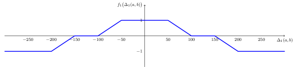
Figure 3: Per-criterion similarity-dissimilarity function $f_{1}$

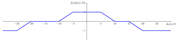
Figure 4: Per-criterion similarity-dissimilarity function $f_{2}$

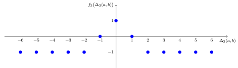
Figure 5: Per-criterion similarity-dissimilarity function $f_{3}$

To get the weights of the elementary criteria and the interaction coefficients, the hierarchical and imprecise SRF method has been applied for each category. In particular, the imprecise SRF method is applied to the set composed by the three macro-criteria as well as to three subsets of the elementary criteria descending from each macro-criterion. Anyway, since the DM provided some information regarding interactions and antagonistic effects between few elementary criteria, we had to adapt the imprecise and hierarchical SRF method as we shall describe in a detailed way in the following.

Suppose that the DM provided the following information:

1. There is a mutual-strengthening effect between $ArMk$ and $PR$;

2. There is a mutual-weakening effect between $PF$ and $TS$;

3. There is an antagonistic effect exercised by $PF$ over $PS$.

Each of the previous three pieces of preference information implies a small modification in the application of the imprecise SRF method:

• In consequence of the first piece of preference information, a mutual-strengthening effect between $MS$ and $MR$ exists too. Therefore, in applying the SRF method at the first level, that is the level composed of criteria $\{MS,MR,PoF\}$, the DM is provided with an additional card with the name of the two criteria $MS$ and $MR$ on, to consider their importance together. Then, the SRF method will be applied to the set composed now of 4 cards $\{MS,MR,\{MS,MR\},PoF\}$. From a technical point of view, in addition to the weights $K_{MS},$ $K_{MR},$ and $K_{PoF}$ representing the importance of criteria $MS$, $MR$ and $PoF$, respectively, we shall take into account also the weight $K({\{MS,MR\}})$. In consequence of the mutual-strengthening effect between $ArMk$ and $PR$, we have that

  $$K({\{MS,MR\}})=K_{MS}+K_{MR}+k_{ArMk,PR},$$

  where $k_{ArMk,PR}>0$ represents, indeed, the value of this effect. Of course, $K({\{MS,MR\}})>K_{MS}$ and $K({\{MS,MR\}})>K_{MR}$;

• Since elementary criteria $PF$ and $TS$ descend from the same macro-criterion $PoF$, the mutual-weakening effect between them is considered adding another card for the pair $\{PF,TS\}$ to take into account their importance together. The imprecise SRF method will be therefore applied to the set $\{PF,M,TS,\{PF,TS\}\}$. The weight of the pair of criteria $\{PF,TS\}$, that is $K(\{PF,TS\})$, will be such that

  $$K(\{PF,TS\})=k_{PF}+k_{TS}+k_{PF,TS}$$

  where, $k_{PF,TS}<0$ is a parameter representing the mutual-weakening effect between them; of course, in consequence of the net flow condition (1), $K({PF,TS})>k_{PF}$ and $K({PF,TS})>k_{TS}$;

• Finally, in consequence of the antagonistic effect exercised by $PF$ over $PS$, the original weight of $PS$ will be reduced. The DM is therefore asked to apply the SRF method to the subset of criteria $\{PS,PS^{{}^{\prime}},PR,PT\}$, where $K(PS^{{}^{\prime}})$ is the importance of criterion $PS$ when $PF$ is exercising its antagonistic effect over it. Consequently, we have

  $$K(PS^{{}^{\prime}})=k_{PS}+k_{PS|PF}$$

  where $k_{PS|PF}<0$ represents the magnitude of the antagonistic effect. In this way, if the DM, for example, in applying the SRF method will order $PS^{{}^{\prime}}$ after $PR$, then this means that $PS$ is more important than $PR$ even if there is another criterion $(PF)$ opposing to it.

In the following we shall describe in detail the application of the hierarchical and imprecise SRF method to the sets of criteria $\{MS,MR,\{MS,MR\},PoF\}$, $\{PF,M,TS,\{PF,TS\}\}$, $\{PS,PS^{{}^{\prime}},PR,PT\}$ and $\{WK,PC,ArMK\}$ for each of the four categories (see also Table 4 summarizing this information).

1. Application of the imprecise SRF method for category $C_{1}$:

   • $PoF$ is less important than $MR$ that is less important than $MS$ that, in turn, is less important than $\{MS,MR\}$. The number of blank cards to be inserted between $\{MS,MR\}$ and $MS$ belongs to the interval $[2,3]$; the number of blank cards between $MS$ and $MR$ varies in the interval $[1,2]$, while there is one blank card between $MR$ and $PoF$. The ratio between the weight of $\{MS,MR\}$ and the weight of $PoF$ belongs to the interval $[4,6]$;

   • With respect to macro-criterion $MS$, $WK$ is less important than $PC$ that, in turn, is less important than $ArMk$. The number of blank cards inserted between $ArMk$ and $PC$ belongs to the interval $[0,2]$, while the number of blank cards inserted between $PC$ and $WK$ has to belong to the interval $[0,1]$. Moreover the ratio between the weight of $ArMk$ and the weight of $WK$ is $3$;

   • Considering macro-criterion $MR$, $PS^{{}^{\prime}}$ is less important than $PS$; $PS$ is less important than $PR$ that, in turn, is less important than $PT$. There is one blank card between $PT$ and $PR$, while the number of blank cards to be inserted between $PR$ and $PS$ has to belong to the interval $[1,2]$. The number of blank cards to be included between $PS$ and $PS^{{}^{\prime}}$ has to belong to the interval $[0,1]$. Finally, the ratio between the weight of $PT$ and that one of $PS^{{}^{\prime}}$ has to belong to the interval $[2,3]$;

   • On macro-criterion $PoF$, $M$ is less important than $PF$ being less important than $TS$ that, in turn, is less important than $\{PF,TS\}$. The number of blank cards between criteria in consecutive ranks varies always in the interval $[1,2]$. The ratio between the weight of the most important criterion ($\{PF,TS\}$) and the least important one $(M)$ varies in the interval $[4,6]$.

2. Application of the imprecise SRF method for category $C_{2}$:

   • $PoF$ is less important than $MS$ that is less important than $MR$ that, in turn, is less important than $\{MR,MS\}$. The number of blank cards to be inserted between $\{MR,MS\}$ and $MR$ belongs to the interval $[2,3]$; there is one blank card between $MR$ and $MS$, while the number of blank cards to be inserted between $MS$ and $PoF$ is in the interval $[1,2]$. Moreover, the ratio between the weight of $\{MR,MS\}$ and the weight of $PoF$ is 6;

   • With respect to macro-criterion $MS$, $WK$ is less important than $PC$ that, in turn, is less important than $ArMk$. There is not any blank card between $ArMk$ and $PC$. The number of blank cards between $PC$ and $WK$ belongs to the interval $[1,2]$. Finally, the ratio between the weight of $ArMk$ and the weight of $WK$ is in the interval $[3,5]$;

   • Considering macro-criterion $MR$, $PS^{{}^{\prime}}$ is less important than $PS$ that is less important than $PR$ that, in turn, is less important than $PT$. The number of blank cards between $PT$ and $PR$ belongs to the interval $[0,1]$. There is not any blank card between $PR$ and $PS$, while the number of blank cards to be inserted between $PS$ and $PS^{{}^{\prime}}$ varies in the interval $[0,1]$. Finally, the ratio between the weight of $PT$ and that one of $PS^{{}^{\prime}}$ has to belong to the interval $[3,4]$;

   • On macro-criterion $PoF$, $PF$ is less important than $M$ that is less important than $TS$ being, in turn, less important than $\{PF,TS\}$. There is one blank card between $\{PF,TS\}$ and $TS$; the number of blank cards between $TS$ and $M$ belongs to the interval $[2,3]$, while the number of blank cards between $M$ and $PF$ varies in the interval $[1,2]$. Finally, the ratio between the weight of the most important criterion ($\{PF,TS\}$) and the least important one $(PF)$ is in the interval $[3,6]$.

3. Application of the imprecise SRF method for category $C_{3}$:

   • $MS$ is less important than $MR$ that is less important than $\{MS,MR\}$ that, in turn, is less important than $PoF$. There is one blank card between $PoF$ and $\{MS,MR\}$. The number of blank cards to be inserted between $\{MS,MR\}$ and $MR$ as well as between $MR$ and $MS$ belongs to the interval $[2,3]$. Finally, the ratio between the weight of $PoF$ and the weight of $MS$ belongs to the interval $[4,6]$;

   • With respect to macro-criterion $MS$, $PC$ is less important than $WK$ that is as important as $ArMk$. There is only one blank card between $PC$ and $ArMk$. Moreover the ratio between the weight of $ArMk$ and the weight of $PC$ is in the interval $[2,4]$;

   • Considering macro-criterion $MR$, $PS^{{}^{\prime}}$ is less important than $PR$ that is less important than $PS$ having the same importance of $PT$. There is one blank card between $PS$ and $PR$, while the number of blank cards between $PR$ and $PS^{\prime}$ belongs to the interval $\left[0,1\right]$. Finally, the ratio between the weight of $PT$ and that one of $PS^{{}^{\prime}}$ has to belong to the interval $[2,4]$;

   • On macro-criterion $PoF$, $TS$ is less important than $PF$ having the same importance of $M$ that, in turn, is less important than the criteria in $\{PF,TS\}$. The number of blank cards between $\{PF,TS\}$ and $PF$ belongs to the interval $[0,1]$. The number of blank cards between $PF$ and $TS$ should vary in the interval $[1,2]$. Finally, the ratio between the weight of $\{PF,TS\}$ and the weight of $TS$ should be in the interval $[3,4]$.

4. Application of the imprecise SRF method for category $C_{4}$:

   • $PoF$ is less important than $MS$ that is less important than $MR$ that, in turn, is less important than $\{MS,MR\}$. The number of blank cards between $\{MS,MR\}$ and $MR$ belongs to the interval $[1,2]$. There is one blank card between $MR$ and $MS$. Moreover, the number of blank cards between $MS$ and $PoF$ should vary in the interval $[1,2]$. Finally, the ratio between the weight of $\{MS,MR\}$ and the weight of $PoF$ is 9;

   • With respect to macro-criterion $MS$, $PC$ and $WK$ are equally important but they are less important than $ArMk$. The number of blank cards that should be inserted between $ArMk$ and the set of criteria $\{PC,WK\}$ belongs to the interval $[1,2]$. Finally, the ratio between the weight of $ArMk$ and the weight of $PC$ is 4;

   • Considering macro-criterion $MR$, $PS^{{}^{\prime}}$ is less important than $PS$ that is less important than $PR$ being less important than $PT$. The number of blank cards between $PT$ and $PR$ belongs to the interval $[0,1]$. There is not any blank card between $PR$ and $PS$ while the number of blank cards between $PS$ and $PS^{\prime}$ belongs to the interval $[0,1]$. Finally, the ratio between the weight of $PT$ and that one of $PS^{{}^{\prime}}$ has to belong to the interval $[2,4]$;

   • On macro-criterion $PoF$, $PF$ is less important than $M$ having the same importance of $TS$ that, in turn, is less important than $\{PF,TS\}$. The number of blank cards between $\{PF,TS\}$ and $M$ belongs to the interval $[1,3]$; the number of blank cards between $M$ and $PF$ varies in the interval $[1,2]$. Finally, the ratio between the weight of $\{PF,TS\}$ and the weight of $PF$ is in the interval $[3,5]$.

Table 4: Data used in the hierarchical and imprecise SRF

	$C_{1}$			$C_{2}$			$C_{3}$			$C_{4}$
Rank	Criterion	No. blank cards	$z$	Criterion	No. blank cards	$z$	Criterion	No. blank cards	$z$	Criterion	No. blank cards	$z$
1	$\{MR,MS\}$	$[2,3]$	$[4,6]$	$\{MS,MR\}$	$[2,3]$	$6$	$PoF$	$1$	$[4,6]$	$\{MS,MR\}$	$[1,2]$	$9$
2	$MS$	$[1,2]$		$MR$	$1$		$\{MS,MR\}$	$[2,3]$		$MR$	$1$
3	$MR$	$1$		$MS$	$[1,2]$		$MR$	$[2,3]$		$MS$	$[1,2]$
4	$PoF$			$PoF$			$MS$			$PoF$
1	$ArMk$	$[0,2]$	$3$	$ArMk$	$0$	$[3,5]$	$WK$, $ArMk$	$1$	$[2,4]$	$ArMk$	$[1,2]$	$4$
2	$PC$	$[0,1]$		$PC$	$[1,2]$		$PC$			$PC$, $WK$
3	$WK$			$WK$
1	$PT$	$1$	$[2,3]$	$PT$	$[0,1]$	$[3,4]$	$PS$, $PT$	$1$	$[2,4]$	$PT$	$[0,1]$	$[2,4]$
2	$PR$	$[1,2]$		$PR$	$0$		$PR$	$[0,1]$		$PR$	$0$
3	$PS$	$[0,1]$		$PS$	$[0,1]$		$PS^{{}^{\prime}}$			$PS$	$[0,1]$
4	$PS^{{}^{\prime}}$			$PS^{{}^{\prime}}$						$PS^{{}^{\prime}}$
1	$\{PF,TS\}$	$[1,2]$	$[4,6]$	$\{PF,TS\}$	$1$	$[3,6]$	$\{PF,TS\}$	$[0,1]$	$[3,4]$	$\{PF,TS\}$	$[1,3]$	$[3,5]$
2	$TS$	$[1,2]$		$TS$	$[2,3]$		$PF$, $M$	$[1,2]$		$M,$ $TS$	$[1,2]$
3	$PF$	$[1,2]$		$M$	$[1,2]$		$TS$			$PF$
3	$M$			$PF$

Introducing all the constraints translating the preference information provided by the DM, we solved the LP problem (11) obtaining $\varepsilon^{*}>0.$ Therefore, there exists at least one set of parameters compatible with the preferences provided by the DM and, consequently, we applied the HAR method to sample 100,000 sets of compatible parameters for each of the four categories.

Now, we shall present in detail all the steps necessary to perform the considered assignments, highlighting the meaning of using the MCHP. For this reason, we consider the soldier $a_{3}$ and the set of sampled weights in Table 5

Table 5: Weights considered in the first part of the example

	$g_{(1,1)}$	$g_{(1,2)}$	$g_{(1,3)}$	$g_{(2,1)}$	$g_{(2,2)}$	$g_{(2,3)}$	$g_{(3,1)}$	$g_{(3,2)}$	$g_{(3,3)}$
$k_{\mathbf{t}}^{1}$	8.925	16.269	26.777	7.537	11.537	14.347	5.312	2.361	8.133
$k_{\mathbf{t}}^{2}$	4.809	12.621	16.140	13.301	16.621	22.599	2.615	4.508	7.274
$k_{\mathbf{t}}^{3}$	5.033	2.304	5.033	12.239	7.082	12.239	23.561	23.561	9.320
$k_{\mathbf{t}}^{4}$	5.557	5.557	22.231	15.011	18.649	22.708	1.838	4.083	4.083

The steps that have to be performed in the assignment procedure are the following:

1. Compute the similarity-dissimilarity: For each elementary criterion and using the three per-criterion similarity-dissimilarity functions introduced above, we compute the similarity-dissimilarity between $a_{3}$ and the four reference actions. The values are shown in Table 6.

   Table 6: Similarity-dissimilarity values for each elementary criterion

   	$g_{(1,1)}$	$g_{(1,2)}$	$g_{(1,3)}$	$g_{(2,1)}$	$g_{(2,2)}$	$g_{(2,3)}$	$g_{(3,1)}$	$g_{(3,2)}$	$g_{(3,3)}$
   $f_{\mathbf{t}}(a_{3},b_{11})$	0	1	0	1	0	0	0.6	0	-1
   $f_{\mathbf{t}}(a_{3},b_{21})$	0	1	1	0	1	1	1	0	1
   $f_{\mathbf{t}}(a_{3},b_{31})$	0	0	0	-1	0	1	-0.6	0	-1
   $f_{\mathbf{t}}(a_{3},b_{41})$	1	1	1	0	1	1	0.6	1	1

2. Compute the comprehensive likeness: Following eqs. (7)-(9), for each non-elementary criterion $g_{\mathbf{r}}$ in the hierarchy, we compute the partial similarity and dissimilarity functions as well as the partial likeness degree between $a_{3}$ and the considered reference actions. The values are shown in Table 7.

   Table 7: Partial similarity, dissimilarity, and likeness degree

   	$s_{\mathbf{1}}^{h}(a_{3},\cdot)$	$d_{\mathbf{1}}(a_{3},\cdot)$	$\delta_{\mathbf{1}}(a_{3},\cdot)$	$s_{\mathbf{2}}^{h}(a_{3},\cdot)$	$d_{\mathbf{2}}(a_{3},\cdot)$	$\delta_{\mathbf{2}}(a_{3},\cdot)$	$s_{\mathbf{3}}^{h}(a_{3},\cdot)$	$d_{\mathbf{3}}(a_{3},\cdot)$	$\delta_{\mathbf{3}}(a_{3},\cdot)$	$s_{\mathbf{0}}^{h}(a_{3},\cdot)$	$d_{\mathbf{0}}(a_{3},\cdot)$	$\delta_{\mathbf{0}}(a_{3},\cdot)$
   $b_{11}$	0.313	0	0.313	0.225	0	0.225	0.201	-1	0	0.266	-1	0
   $b_{21}$	0.856	0	0.856	0.746	0	0.543	0.668	0	0.668	0.773	0	0.773
   $b_{31}$	0	0	0	0.387	-1	0	0	-1	0	0	-1	0
   $b_{41}$	1	0	1	0.733	0	0.733	0.926	0	0.926	0.842	0	0.842

   For example, to compute $s_{\mathbf{3}}^{h}(a_{3},b_{11})$ w.r.t. category $C_{1}$, that is the similarity between $a_{3}$ and $b_{11}$ on $PoF$ ($g_{\mathbf{3}}$) for assigning $a_{3}$ to snipers, we have to take into account only the last three elementary criteria as well as the mutual-strengthening effect between $PF$ ($g_{(\mathbf{3},1)}$) and $TS$ ($g_{(\mathbf{3},3)}$). In particular, observing that $d_{\mathbf{t}}(a_{3},b_{11})=f_{\mathbf{t}}(a_{3},b_{11})$ if $f_{\mathbf{t}}(a_{3},b_{11})<0$ and 0 otherwise, and that $s_{\mathbf{t}}(a_{3},b_{11})=f_{\mathbf{t}}(a_{3},b_{11})$ if $f_{\mathbf{t}}(a_{3},b_{11})>0$ and 0 otherwise, we have that $s_{(\mathbf{3},1)}(a_{3},b_{11})=f_{(\mathbf{3},1)}(a_{3},b_{11})$ and $d_{(\mathbf{3},3)}(a_{3},b_{11})=f_{(\mathbf{3},3)}(a_{3},b_{11})$. We obtain:

   • $K_{\mathbf{3}}^{{h}}(a,b_{11})=k_{(\mathbf{3},1)}^{1}+k_{(\mathbf{3},2)}^{1}+k_{(\mathbf{3},3)}^{1}=5.312+2.361+8.133=15.806;$

   • $s_{\mathbf{3}}^{h}(a_{3},b_{11})=\frac{k_{(\mathbf{3},1)}^{{1}}\cdot f_{(\mathbf{3},1)}(a_{3},b_{11})}{K_{\mathbf{3}}^{h}(a,b_{11})}=\frac{5.312\cdot 0.6}{15.806}=0.2016;$

   • $d_{\mathbf{3}}(a_{3},b_{11})=\left(1+d_{(\mathbf{3},3)}(a_{3},b_{11})\right)-1=d_{(\mathbf{3},3)}(a_{3},b_{11})=-1$;

   • $\delta_{\mathbf{3}}(a_{3},b_{11})=s_{\mathbf{3}}^{h}(a_{3},b_{11})\left(1+d_{\mathbf{3}}(a_{3},b_{11})\right)=0.2016\cdot(1-1)=0.$

   The other values in Table 7 are computed analogously.

3. Assignment procedure: For each non-elementary criterion $g_{\mathbf{r}}$, and for each category $C_{h}$, a likeness threshold $\lambda_{\mathbf{r}}^{h}$ has to be defined. In this case, we are assuming that the likeness thresholds are the same for each $g_{\mathbf{r}}$ and these values are shown in Table 8.

   Table 8: Likeness threshold for the four categories

   	$h=1$	$h=2$	$h=3$	$h=4$
   $\lambda_{\mathbf{r}}^{h}$	0.65	0.60	0.65	0.60

   Comparing the partial likeness degree $\delta_{\mathbf{r}}(a_{3},\cdot)$ with the corresponding likeness threshold $\lambda_{\mathbf{r}}^{h}$ for each non-elementary criterion $g_{\mathbf{r}}$, soldier $a_{3}$ can be assigned to the categories shown in Table 9.

   Table 9: Assignments of $a_{3}$ on each non-elementary criterion

   	$\delta_{\mathbf{1}}(a_{3},\cdot)$	$\lambda_{\mathbf{1}}^{h}$		$\delta_{\mathbf{2}}(a_{3},\cdot)$	$\lambda_{\mathbf{2}}^{h}$		$\delta_{\mathbf{3}}(a_{3},\cdot)$	$\lambda_{\mathbf{3}}^{h}$		$\delta_{\mathbf{0}}(a_{3},\cdot)$	$\lambda_{\mathbf{0}}^{h}$
   $b_{11}$	0.313	0.65		0.225	0.65		0	0.65		0	0.65
   $b_{21}$	0.856	0.60	✓	0.543	0.60	✓	0.668	0.60	✓	0.773	0.60	✓
   $b_{31}$	0	0.65		0	0.65		0	0.65		0	0.65
   $b_{41}$	1	0.60	✓	0.733	0.60	✓	0.926	0.60	✓	0.842	0.60	✓

7.2 Application of the SMAA to the hCat-SD method

Considering the likeness thresholds for each category shown in Table 8, and assuming that they are the same for each non-elementary criterion $g_{\mathbf{r}}$, we applied the hCat-SD method for each sampled set of compatible parameters. Therefore, we were able to compute the probability of assigning each soldier to the considered categories reported in Table 10.

Table 10: Probability of assignments expressed in percentage

Soldier	$C_{1}$	$C_{2}$	$C_{3}$	$C_{4}$	$\{C_{2},C_{4}\}$	$C_{5}$
$a_{1}$	100	0	0	0	0	0
$a_{2}$	0	0	0	0	100	0
$a_{3}$	0	0	0	0	100	0
$a_{4}$	0	0	100	0	0	0
$a_{5}$	0	100	0	0	0	0
$a_{6}$	100	0	0	0	0	0
$a_{7}$	0	0	0	0	100	0

(a) Comprehensive level

Soldier	$C_{1}$	$C_{2}$	$C_{3}$	$C_{4}$	$\{C_{1},C_{3}\}$	$\{C_{2},C_{4}\}$	$C_{5}$
$a_{1}$	0	0	0	0	100	0	0
$a_{2}$	0	100	0	0	0	0	0
$a_{3}$	0	0	0	0	0	100	0
$a_{4}$	0	0	0	0	0	0	100
$a_{5}$	0	0	0	0	0	100	0
$a_{6}$	100	0	0	0	0	0	0
$a_{7}$	0	0	0	0	0	100	0

(b) Mental Sharpness $(MS)$

Soldier	$C_{1}$	$C_{2}$	$C_{3}$	$C_{4}$	$\{C_{2},C_{4}\}$	$\{C_{2},C_{3},C_{4}\}$	$C_{5}$
$a_{1}$	100	0	0	0	0	0	0
$a_{2}$	0	0	0	0	100	0	0
$a_{3}$	0	0	0	0	100	0	0
$a_{4}$	0	0	0	0	0	100	0
$a_{5}$	0	0	0	0	100	0	0
$a_{6}$	100	0	0	0	0	0	0
$a_{7}$	0	0	0	0	100	0	0

(c) Mental Resilience ($MR$)

Soldier	$C_{1}$	$C_{2}$	$C_{3}$	$C_{4}$	$\{C_{2},C_{4}\}$	$C_{5}$
$a_{1}$	100	0	0	0	0	0
$a_{2}$	0	0	0	0	100	0
$a_{3}$	0	0	0	0	100	0
$a_{4}$	0	0	97.269	0	0	2.731
$a_{5}$	0	100	0	0	0	0
$a_{6}$	100	0	0	0	0	0
$a_{7}$	0	0	0	100	0	0

(d) Physical and other Features ($PoF$)

Looking at Tables 11(a)-11(d) one can observe that the results are quite stable, that is, the frequency of assignment is very close to 100% in almost all cases. This is due to the fact that the preference information provided by the DM was quite precise and, consequently, the space of parameters compatible with this information was quite narrow. However, one can observe the following:

• At comprehensive level (Table 11(a)), all candidates are assigned to at least one category. In particular, $a_{1}$ and $a_{6}$ are surely suitable to be snipers ($C_{1}$), $a_{5}$ sure be assigned to the breachers ($C_{2}$), $a_{3}$ is surely suitable to be a communication operator ($C_{3}$), while the other three candidates, that is $a_{2}$, $a_{3}$ and $a_{7}$, can be indifferently included among breachers or heavy weapons operators ($\{C_{2},C_{4}\}$);

• With respect to $MS$, only two candidates can be assigned with certainty to a unique category. In particular, $a_{2}$ is always assigned to breachers category ($C_{2}$) and $a_{6}$ is always assigned to snipers $(C_{1})$; regarding the remaining candidates, $a_{1}$ can cover indifferently both snipers and communications operators $(\{C_{1},C_{3}\})$, $a_{3}$, $a_{5}$ and $a_{7}$ can be included in breachers and heavy weapons operator categories simultaneously $(\{C_{2},C_{4}\})$; finally, $a_{4}$ is not idoneous to any of the considered categories;

• On $MR$, all candidates are assigned with certainty to at least one category. $a_{1}$ and $a_{6}$ are idoneous to be included in the snipers category $(C_{1})$; $a_{4}$ has evaluations such that he can be included indifferently in all categories apart from snipers one $(\{C_{2},C_{3},C_{4}\})$; finally, all the other candidates ($a_{2}$, $a_{3}$, $a_{5}$ and $a_{7}$) can be breachers or heavy weapons operators indifferently $(\{C_{2},C_{4}\})$;

• Considering $PoF$, there is a better distribution of the candidates among the different categories: $a_{1}$ and $a_{6}$ are assigned with certainty to the snipers $(C_{1})$; $a_{5}$ is surely assigned to the breachers $(C_{2})$; $a_{4}$ is included among the communication operators $(C_{3})$ with a frequency of the $97.269\%$, while he is not assigned to any category in the remaining cases; $a_{7}$ is certainly idoneous to be included in the heavy weapons operators category $(C_{4})$. The remaining two candidates, that is $a_{2}$ and $a_{3}$ can be indifferently assigned to the breachers and heavy weapons operators categories ($\{C_{2},C_{4}\}$).

7.3 A deterministic nominal classification respecting some specified requirements

To conclude this section, we shall show how the classification procedure described in Section 6 can be applied to this problem to get a deterministic nominal classification taking into account the results obtained by using the SMAA methodology and the following additional requirements that are specified by the DM for each non-elementary criterion $g_{\mathbf{r}}$:

R1)

Each soldier should be assigned to a single category or to the dummy one;

R2)

At least one soldier should be assigned to each $C_{h}$, $h=1,\ldots,4$;

R3)

At most two soldiers should be assigned to each $C_{h}$, $h=1,\ldots,4$;

R4)

At most two soldiers should not be assigned (at most two soldiers should be assigned to the dummy category $C_{5}$).

Taking into account the SMAA results given in tables 11(a)-11(d), one deterministic nominal classification can be obtained for each non-elementary criterion. Anyway, in the following we shall explain in detail how to get the deterministic nominal classification at comprehensive level, that is considering $g_{\mathbf{0}}$.

Looking at Table 11(a) we observe that $a_{2}$, $a_{3}$ and $a_{7}$ can be always simultaneously assigned to categories $C_{2}$ and $C_{4}$. Therefore, since we would like to consider a nominal classification assigning soldiers to one among $C_{1}-C_{4}$ or to the dummy category $C_{5}$ we rewrite the table 11(a) as shown in Table 11.

Table 11: Frequencies of assignments at comprehensive level

Soldier	$C_{1}$	$C_{2}$	$C_{3}$	$C_{4}$	$C_{5}$
$a_{1}$	100	0	0	0	0
$a_{2}$	0	100	0	100	0
$a_{3}$	0	100	0	100	0
$a_{4}$	0	0	100	0	0
$a_{5}$	0	100	0	0	0
$a_{6}$	100	0	0	0	0
$a_{7}$	0	100	0	100	0

Considering that, in this case, $A=\{a_{1},\ldots,a_{7}\}$, a deterministic nominal classification taking into account the probabilistic information given by the SMAA methodology and the requirements provided by the DM, one has to solve the following LP problem where all variables are binary and constraints $[C1]-[C4]$ translate the requirements provided by the DM:

$$\begin{array}[]{l}\min L(\mathbf{y}_{\mathbf{0}})={\displaystyle\sum_{a\in A}\sum_{h=1}^{5}y_{a,\mathbf{0}}^{h}\sum_{k\neq h}b_{\mathbf{0}}^{k}(a),\;\;\mbox{subject to}}\\[5.69054pt] \left.\begin{array}[]{ll}\mbox{for each $a\in A$}\;\;{\displaystyle\sum_{h=1}^{5}y_{a,\mathbf{0}}^{h}=1}&[C1]\\[5.69054pt] \mbox{for each $h=1,\ldots,4$}\;\;{\displaystyle\sum_{a\in A}y_{a,\mathbf{0}}^{h}\geqslant 1}&[C2]\\[5.69054pt] \mbox{for each $h=1,\ldots,4$}\;\;{\displaystyle\sum_{a\in A}y_{a,\mathbf{0}}^{h}\leqslant 2}&[C3]\\[5.69054pt] {\displaystyle\sum_{a\in A}y_{a,\mathbf{0}}^{5}\leqslant 2}&[C4]\\[8.53581pt] y_{a,\mathbf{0}}^{h}\in\{0,1\},\;\forall a\in A,\;\forall h=1,\ldots,5.\end{array}\right\}E^{LF}\end{array}$$ (15)

Solving the LP (15), we get $y_{1,\mathbf{0}}^{1,*}=y_{2,\mathbf{0}}^{4,*}=y_{3,\mathbf{0}}^{2,*}=y_{4,\mathbf{0}}^{3,*}=y_{5,\mathbf{0}}^{2,*}=y_{6,\mathbf{0}}^{1,*}=y_{7,\mathbf{0}}^{4,*}=1$, while all the other binary variables are equal to zero. This means that the deterministic nominal classification shown in the first column of Table 12 is therefore obtained.

Table 12: Deterministic nominal classifications obtained at comprehensive level

Soldier	$1st$	$2nd$	$3rd$
$a_{1}$	$C_{1}$	$C_{1}$	$C_{1}$
$a_{2}$	$C_{4}$	$C_{2}$	$C_{4}$
$a_{3}$	$C_{2}$	$C_{4}$	$C_{4}$
$a_{4}$	$C_{3}$	$C_{1}$	$C_{3}$
$a_{5}$	$C_{2}$	$C_{2}$	$C_{2}$
$a_{6}$	$C_{1}$	$C_{1}$	$C_{1}$
$a_{7}$	$C_{4}$	$C_{4}$	$C_{2}$

To check for the existence of another deterministic nominal classification, considering that the optimal value of the loss function previously found is $L_{\mathbf{y}_{\mathbf{0}}^{*}}=300$, one has to solve the same LP problem (15) with the addition of the constraints

$$\begin{array}[]{ll}L(\mathbf{y}_{\mathbf{0}})=300&[C1^{\prime}]\\[5.69054pt] y_{1,\mathbf{0}}^{1}+y_{2,\mathbf{0}}^{4}+y_{3,\mathbf{0}}^{2}+y_{4,\mathbf{0}}^{3}+y_{5,\mathbf{0}}^{2}+y_{6,\mathbf{0}}^{1}+y_{7,\mathbf{0}}^{4}\leqslant 6&[C2^{\prime}]\\[5.69054pt] \end{array}$$

where $[C1^{\prime}]$ imposes that the optimal value of the loss function should not be deteriorated, while $[C2^{\prime}]$ ensures that the previous solutions of the problem is not found anymore. By proceeding in this way, one gets $y_{1,\mathbf{0}}^{1,*}=y_{2,\mathbf{0}}^{2,*}=y_{3,\mathbf{0}}^{4,*}=y_{4,\mathbf{0}}^{3,*}=y_{5,\mathbf{0}}^{2,*}=y_{6,\mathbf{0}}^{1,*}=y_{7,\mathbf{0}}^{4,*}=1$ that provides the deterministic nominal classification shown in the second column of Table 12. Proceeding analogously, we find only another deterministic nominal classification summarizing the results obtained by the application of the SMAA methodology and compatible with the requirements provided by the DM that is shown in the last column of Table 12.

A similar procedure can be used to obtain the deterministic nominal classifications w.r.t. each of the three macro-criteria. We will not give the detail of the computations in these cases but the obtained classifications are shown in Tables 14(a)-14(c).

Table 13: Deterministic nominal classification at partial level

Soldier	$1st$	$2nd$	$3rd$
$a_{1}$	$C_{3}$	$C_{3}$	$C_{3}$
$a_{2}$	$C_{2}$	$C_{2}$	$C_{2}$
$a_{3}$	$C_{2}$	$C_{4}$	$C_{4}$
$a_{4}$	$C_{5}$	$C_{5}$	$C_{5}$
$a_{5}$	$C_{4}$	$C_{4}$	$C_{2}$
$a_{6}$	$C_{1}$	$C_{1}$	$C_{1}$
$a_{7}$	$C_{4}$	$C_{2}$	$C_{4}$

(a) Mental Sharpness $(MS)$

Soldier	$1st$	$2nd$	$3rd$	$4th$	$5th$	$6th$
$a_{1}$	$C_{1}$	$C_{1}$	$C_{1}$	$C_{1}$	$C_{1}$	$C_{1}$
$a_{2}$	$C_{2}$	$C_{4}$	$C_{2}$	$C_{4}$	$C_{4}$	$C_{2}$
$a_{3}$	$C_{2}$	$C_{2}$	$C_{4}$	$C_{4}$	$C_{2}$	$C_{4}$
$a_{4}$	$C_{3}$	$C_{3}$	$C_{3}$	$C_{3}$	$C_{3}$	$C_{3}$
$a_{5}$	$C_{4}$	$C_{4}$	$C_{4}$	$C_{2}$	$C_{2}$	$C_{2}$
$a_{6}$	$C_{1}$	$C_{1}$	$C_{1}$	$C_{1}$	$C_{1}$	$C_{1}$
$a_{7}$	$C_{4}$	$C_{2}$	$C_{2}$	$C_{2}$	$C_{4}$	$C_{4}$

(b) Mental Resilience ($MR$)

Soldier	$1st$	$2nd$
$a_{1}$	$C_{1}$	$C_{1}$
$a_{2}$	$C_{4}$	$C_{2}$
$a_{3}$	$C_{2}$	$C_{4}$
$a_{4}$	$C_{3}$	$C_{3}$
$a_{5}$	$C_{2}$	$C_{2}$
$a_{6}$	$C_{1}$	$C_{1}$
$a_{7}$	$C_{4}$	$C_{4}$

(c) Physical and other Features ($PoF$)

8 Conclusions

In this paper, we proposed a comprehensive method extending a recently proposed nominal classification, the Cat-SD method. Firstly, we applied MCHP to the Cat-SD method. Thus, we have introduced the hierarchical Cat-SD, hCat-SD. The hierarchical decomposition of a complex multiple criteria nominal classification problem is then possible when applying Cat-SD. Secondly, interactions and antagonistic effects between criteria structured in a hierarchical way were handled in our method. Then, to elicit the values of the criteria weights as well as the interactions and antagonistic coefficients used in the hCat-SD method, we proposed a new development of the hierarchical and imprecise SRF method. We applied SMAA to the hCat-SD method with the aim of obtaining the probablity with which an action is assigned to a category (or categories) at a comprehensive level and at a macro-criterion level. Finally, considering the concept of loss function, we proposed a procedure that starting from the probabilistic assignments obtained by SMAA provides a final classification that fulfills some requirements given by the DM. Putting together all these aspects, we therefore built the SMAA-hCat-SD method. We presented a numerical example to illustrate the application of SMAA-hCat-SD.

The proposed method gives to the DM the possibility:

• To structure the set of criteria in a hierarchical way (logical subsets of criteria can be created in the hierarchy);

• To provide imprecise information for obtaining the criteria weights as well as the interaction and antagonistic coefficients by using the imprecise SRF method;

• To analyze, for several sets of compatible parameters, the probability of the assignment results provided by the Cat-SD, considering all criteria or one macro-criterion only;

• To obtain a final assignment that takes into account robustness concerns as represented by the probabilistic classification provided by SMAA.

Several advantages can be underlined with respect to the application of the proposed method. The main features can be stated as follows:

1. In situations in which the DM has to handle a great number of criteria to assess actions, adopting hCat-SD is a more adequate approach than applying Cat-SD considering all criteria at the same level;

2. For the elicitation of the criteria weights and interaction and antagonistic coefficients, it is easier for the DM thinking about a small number of related criteria than a large number;

3. Besides the possibility of eliciting criteria weights for subsets of criteria, our method gives to the DM the possibility to provide imprecise information during the process of determining them;

4. Applying SMAA to the hCat-SD, the DM can better understand the decision problem at hand exploring the problem more in deep.

To sum up, in this work we have considered robustness concerns by taking into account the set of all weights and interaction and antagonistic coefficients compatible with preference information provided by the DM, while taking advantage of the hierarchical structure of criteria. Let us remark that:

• The extension of the SRF method to elicit weights of criteria as well as interaction and antagonistic coefficients can be applied to all Electre methods and, more in general, to all outranking methods;

• The procedure permitting to pass from the probabilistic classification provided by SMAA to the final assignment can be applied to other probabilistic versions of classification methods, also ordinal, such as Electre Tri and its variants.

Future research can rely on applying the SMAA-hCat-SD method to real-world nominal classification problems. Extending the method to group decision making is also an interesting direction of research. It could also be interesting to study procedures for aiding the elicitation of preference information given by the DM to reduce the cognitive effort required during the decision aiding process.

References

- Angilella et al. (2016) Angilella, S., Corrente, S., Greco, S., Słowiński, R., 2016. Robust Ordinal Regression and Stochastic Multiobjective Acceptability Analysis in multiple criteria hierarchy process for the Choquet integral preference model. Omega 63, 154–169.
- Arcidiacono et al. (2018) Arcidiacono, S.G., Corrente, S., Greco, S., 2018. GAIA-SMAA-Promethee for a hierarchy of interacting criteria. European Journal of Operational Research 270, 606–624.
- Belacel (2000) Belacel, N., 2000. Multicriteria assignment method PROAFTN: Methodology and medical application. European Journal of Operational Research 125, 175–183.
- Belton and Stewart (2002) Belton, V., Stewart, T., 2002. Multiple Criteria Decision Analysis: An Integrated Approach. Kluwer Academic Publishers, Dordrecht, The Netherlands.
- Bottero et al. (2015) Bottero, M., Ferretti, V., Figueira, J., Greco, S., Roy, B., 2015. Dealing with a multiple criteria environmental problem with interaction effects between criteria through an extension of the Electre III method. European Journal of Operational Research 245, 837–850.
- Casasanto and Lupyan (2015) Casasanto, D., Lupyan, G., 2015. All concepts are ad hoc concepts, in: Margolis, E., Laurence, S. (Eds.), The conceptual mind: New directions in the study of concepts. MIT Press, Cambridge, MA, pp. 543–566.
- Corrente et al. (2017a) Corrente, S., Doumpos, M., Greco, S., Słowiński, R., Zopounidis, C., 2017a. Multiple criteria hierarchy process for sorting problems based on ordinal regression with additive value functions. Annals of Operations Research 251, 117–139.
- Corrente et al. (2017b) Corrente, S., Figueira, J., Greco, S., Słowiński, R., 2017b. A robust ranking method exending Electre III to hierarchy of interacting criteria, imprecise weights and stochastic analysis. Omega 73, 1–17.
- Corrente et al. (2013a) Corrente, S., Greco, S., Kadziński, M., Słowiński, R., 2013a. Robust ordinal regression in preference learning and ranking. Machine Learning 93, 381–422.
- Corrente et al. (2019) Corrente, S., Greco, S., Nicotra, M., Romano, M., Schillaci, C.E., 2019. Evaluating and comparing entrepreneurial ecosystems using SMAA and SMAA-S. The Journal of Technology Transfer 44, 485–519.
- Corrente et al. (2012) Corrente, S., Greco, S., Słowiński, R., 2012. Multiple criteria hierarchy process in robust ordinal regression. Decision Support Systems 53, 660–674.
- Corrente et al. (2013b) Corrente, S., Greco, S., Słowiński, R., 2013b. Multiple criteria hierarchy process with Electre and Promethee. Omega 41, 820–846.
- Corrente et al. (2016) Corrente, S., Greco, S., Słowiński, R., 2016. Multiple criteria hierarchy process for Electre Tri methods. European Journal of Operational Research 252, 191–203.
- Costa et al. (2018) Costa, A., Figueira, J.R., Borbinha, J., 2018. A multiple criteria nominal classification method based on the concepts of similarity and dissimilarity. European Journal of Operational Research 271, 193–209.
- Costa et al. (2019a) Costa, A., Figueira, J.R., Borbinha, J., 2019a. A multiple criteria nominal classification method in a web-based platform: Demonstration in a case of recruitment for the portuguese army. arXiv arXiv:1904.04128.
- Costa et al. (2019b) Costa, A.S., Lami, I.M., Greco, S., Figueira, J.R., Borbinha, J., 2019b. A multiple criteria approach defining cultural adaptive reuse of abandoned buildings, in: Huber, S. Geiger, M., de Almeida, A. (Eds.), Multiple Criteria Decision Making and Aiding - Cases on Decision Making Methods and Models with Computer Implementations. Springer, Cham, Switzerland, pp. 193–218.
- Doumpos and Zopounidis (2002) Doumpos, M., Zopounidis, C., 2002. Multicriteria Decision Aid Classification Methods. Kluwer Academic Publishers, Dordrecht, The Netherlands.
- Figueira et al. (2009) Figueira, J., Greco, S., Roy, B., 2009. Electre methods with interaction between criteria: An extension of the concordance index. European Journal of Operational Research 199, 478–495.
- Figueira and Roy (2002) Figueira, J., Roy, B., 2002. Determining the weights of criteria in the Electre type methods with a revised Simos’ procedure. European Journal of Operational Research 139, 317–326.
- Furems (2013) Furems, E.M., 2013. Dominance-based extension of Stepclass for multiattribute nominal classification. International Journal of Information Technology & Decision Making 12, 905–925.
- Gneiting and Raftery (2007) Gneiting, T., Raftery, A.E., 2007. Strictly proper scoring rules, prediction, and estimation. Journal of the American Statistical Association 102, 359–378.
- Greco et al. (2016) Greco, A., Figueira, J., Ehrgott, M., 2016. Multiple Criteria Decision Analysis: State of the Art Surveys. Springer Science+Business Media, New York, NY. 2nd edition.
- Henriet (2000) Henriet, L., 2000. Systèmes d’Évaluation et de Classification Multicritères pour l’Aide à la Décision: Construction de Modèles et Procédures d’Affectation. Ph.D. thesis. Université Paris-Dauphine. Paris, France.
- Ishizaka and Nemery (2013) Ishizaka, A., Nemery, P., 2013. Multicriteria Decision Aid: Methods and Software. John Wiley & Sons, Ltd., Chichester, UK.
- Kadziński et al. (2015) Kadziński, M., Ciomek, K., Słowiński, R., 2015. Modeling assignment-based pairwise comparisons within integrated framework for value-driven multiple criteria sorting. European Journal of Operational Research 241, 830 – 841.
- Kadziński and Słowiński (2013) Kadziński, M., Słowiński, R., 2013. DIS-CARD: A new method of multiple criteria sorting to classes with desired cardinality. Journal of Global Optimization 56, 1143–1166.
- Lahdelma et al. (1998) Lahdelma, R., Hokkanen, J., Salminen, P., 1998. SMAA - Stochastic multiobjective acceptability analysis. European Journal of Operational Research 106, 137–143.
- Lahdelma and Salminen (2010) Lahdelma, R., Salminen, P., 2010. Stochastic multicriteria acceptability analysis (SMAA), in: Ehrgott, M., Figueira, J., Greco, S. (Eds.), Trends in Multiple Criteria Decision Analysis, Springer Science+Business Media LLC, New York, NY. pp. 321–354.
- Léger and Martel (2002) Léger, J., Martel, J.M., 2002. A multicriteria assignment procedure for a nominal sorting problematic. European Journal of Operational Research 138, 349–364.
- Mousseau et al. (2003a) Mousseau, V., Dias, L., Figueira, J., 2003a. On the notion of category size in multiple criteria sorting models. Cahier du LAMSADE 205.
- Mousseau et al. (2003b) Mousseau, V., Figueira, J., Dias, L., Gomes da Silva, C., Clímaco, J., 2003b. Resolving inconsistencies among constraints on the parameters of an MCDA model. European Journal of Operational Research 147, 72–93.
- Özpeynirci et al. (2018) Özpeynirci, S., Özpeynirci, Ö., Mousseau, V., 2018. An interactive algorithm for multiple criteria constrained sorting problem. Annals of Operations Research 267, 447–466.
- Pelissari et al. (2019) Pelissari, R., Oliveira, M., Amor, S.B., Kandakoglu, A., Helleno, A., 2019. SMAA methods and their applications: A literature review and future research directions. Annals of Operations Research DOI: 10.1007/s10479-019-03151-z.
- Perny (1998) Perny, P., 1998. Multicriteria filtering methods based on concordance and non-discordance principles. Annals of Operations Research 80, 137–165.
- Rigopoulos et al. (2010) Rigopoulos, G., Askounis, D.T., Metaxiotis, K., 2010. NexCLass: A decision support system for non-ordered multicriteria classification. International Journal of Information Technology & Decision Making 9, 53–79.
- Savage (1971) Savage, L.J., 1971. Elicitation of personal probabilities and expectations. Journal of the American Statistical Association 66, 783–801.
- Schervish (1989) Schervish, M., 1989. A general method for comparing probability assessors. The Annals of Statistics 17, 1856–1879.
- Simos (1990a) Simos, J., 1990a. Evaluer l’impact sur l’environnement: Une approche originale par l’analyse multicritère et la négociation, Presses Polytechniques et Universitaires Romandes, Lausanne.
- Simos (1990b) Simos, J., 1990b. L’Évaluation Environnementale: Un Processus Cognitif Négocié. Ph.D. thesis. DGF-EPFL, Lausanne, Suisse.
- Słowiński and Vanderpooten (2000) Słowiński, R., Vanderpooten, D., 2000. A generalized definition of rough approximations based on similarity. IEEE Transactions on Knowledge and Data Engineering 12, 331–336.
- Smith (1984) Smith, R., 1984. Efficient Monte Carlo procedures for generating points uniformly distributed over bounded regions. Operations Research 32, 1296–1308.
- Stal-Le Cardinal et al. (2011) Stal-Le Cardinal, J., Mousseau, V., Zheng, J., 2011. An application of constrained multicriteria sorting to student selection, in: Salo, A., Keisler, J., Morton, A. (Eds.), Portfolio Decision Analysis. Springer, New York, NY, pp. 213–240.
- Taskar et al. (2001) Taskar, B., Segal, E., Koller, D., 2001. Probabilistic classification and clustering in relational data, in: International joint conference on artificial intelligence, Lawrence Erlbaum Associates LTD. pp. 870–878.
- Tervonen et al. (2013) Tervonen, T., Van Valkenhoef, G., Bastürk, N., Postmus, D., 2013. Hit-and-run enables efficient weight generation for simulation-based multiple criteria decision analysis. European Journal of Operational Research 224, 552–559.
- Van Valkenhoef et al. (2014) Van Valkenhoef, G., Tervonen, T., Postmus, D., 2014. Notes on “Hit-And-Run enables efficient weight generation for simulation-based multiple criteria decision analysis”. European Journal of Operational Research 239, 865–867.
- Williams and Barber (1998) Williams, C.K., Barber, D., 1998. Bayesian classification with gaussian processes. IEEE Transactions on Pattern Analysis and Machine Intelligence 20, 1342–1351.
- Zopounidis and Doumpos (2002) Zopounidis, C., Doumpos, M., 2002. Multicriteria classification and sorting methods: A literature review. European Journal of Operational Research 138, 229–246.