Response of active Brownian particles to shear flow

Abstract

We study the linear response of interacting active Brownian particles in an external potential to simple shear flow. Using a path integral approach, we derive the linear response of any state observable to initiating shear in terms of correlation functions evaluated in the unperturbed system. For systems and observables which are symmetric under exchange of the $x$ and $y$ coordinates, the response formula can be drastically simplified to a form containing only state variables in the corresponding correlation functions (compared to the generic formula containing also time derivatives). In general, the shear couples to the particles by translational as well as rotational advection, but in the aforementioned case of $xy$ symmetry only translational advection is relevant in the linear regime. We apply the response formulas analytically in solvable cases and numerically in a specific setup. In particular, we investigate the effect of a shear flow on the morphology and the stress of $N$ confined active particles in interaction, where we find that the activity as well as additional alignment interactions generally increase the response.

I Introduction

Many systems found in nature are inherently open and thus operate out of equilibrium. Among them, active systems are driven by energy dissipation at the level of each of their individual components. This strong form of driving at the small scale leads to original collective behaviors at larger scales, from flocking [1, 2] to spontaneous bacterial flows [3, 4] and many more (see, e.g., Refs. [5, 6, 7] for recent reviews).

To better comprehend and manipulate active matter, it is important to understand how it responds to external perturbations. The response of a system to shear is of particular interest since it tells us about the rheology of the fluid under consideration [8, 9]. In that respect, active fluids exhibit surprising properties. In particular, the dipolar forces exerted by swimmers in a solution can lead to an increase [10] or a decrease in viscosity [11], even turning the solution into a superfluid [12]. This may be of particular relevance for blood flow [13].

The rheology of active fluids can be understood qualitatively through analytic arguments [14, 15] and numerical simulations [16, 17] but the quantitative prediction of transport coefficients remains mostly out of reach. To this aim, response relations are particularly useful since they allow to compute the average response of a system in terms of correlation functions in the unperturbed system. When considering perturbations of an equilibrium system, these are the celebrated fluctuation-dissipation theorems [18, 19, 20] and Green-Kubo relations [21, 20, 22]. Extending such relations to describe the perturbation of nonequilibrium steady states has been the subject of intense research [23, 24, 25, 26, 27, 28, 29, 30, 31, 32, 33, 34, 35] and is the topic of the present article. Note that activity itself is sometimes treated as a perturbation parameter [36, 37, 38]. This is not the case here as we consider perturbations close to nonequilibrium steady states with potentially high activity.

In this work, we study the linear response to shear of a collection of active, i.e., self-propelled, Brownian particles (ABPs). This model of “dry” active matter (neglecting the effect of a solvent) has become a workhorse for studying active systems [6, 7], including important phenomena such as motility induced phase separation [39] which was also found for colloidal swimmers [40]. The microscopic mechanisms of swimming motion, and the effects of hydrodynamic interactions are yet a diverse field of research, see, e.g., Refs. [5, 6, 41, 42, 43, 44, 45, 46].

Using path integral techniques, we derive here a general formula, valid for any interaction and external potentials, to compute the linear response to shear in terms of correlation functions evaluated in the unsheared system. In the special case where the situation is symmetric under exchange of the $x$ and $y$ axes, the response formula simplifies such that it contains only static variables (no velocities) and is not affected by shear rotation. As we show, the formula recovers results previously derived in the literature for one ABP in a shear flow in free space [47] or confined by a harmonic potential [48]. Our work complements that of Ref. [49], which derived, in another model of active particles, a response relation for perturbations via a potential (not shear). Further, we apply our response formula to $N$ interacting particles confined in a harmonic potential in two space dimensions. We compute the average of $\sum_{i=1}^{N}x_{i}y_{i}$, where $(x_{i},y_{i})$ is the position of particle $i$, to quantify the effect of shear on the morphology of the suspension. We also numerically check the consistency of our results, and therefore the response formula, by computing the response directly in the sheared system.

The paper is organized as follows. In Sec. II, we describe the model and introduce relevant physical quantities. Section III contains a detailed derivation and discussion of the response formulas. The formulas are then applied analytically to single-particle systems in Sec. IV, and numerically to a many-body situation in Sec. V. We close this manuscript by a summary and conclusions in Sec. VI.

II System and Model

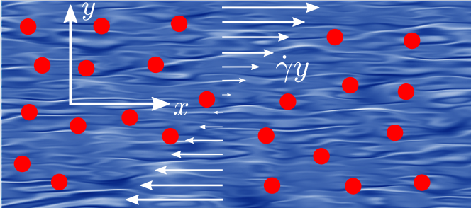
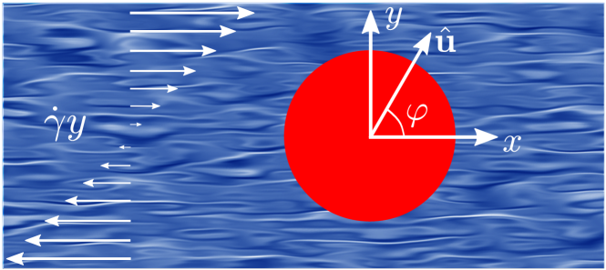
Figure 1: The system under consideration: interacting active Brownian particles (red circles) exposed to simple shear flow (white arrows) with shear velocity $\dot{\gamma}y$. Top: Schematic representation of $N$ particles. Bottom: Schematic representation of a single particle with heading $\hat{\mathbf{u}}$.

We consider $N$ overdamped active Brownian particles, subject to interactions and external forces. For simplicity, we provide the derivation and explicit examples for a two-dimensional system, which is relevant to many experiments [50, 51, 52, 53]. The generalization to ABPs in 3D and also to more general active particle models is given in Subsec. III.5. Each particle thus has three degrees of freedom: two translational (in the $x$ and $y$ directions) and an angle $\varphi$ parametrizing its heading $\hat{\mathbf{u}}(\varphi)=\left(\cos(\varphi),\sin(\varphi)\right)^{T}$ in which the particle self-propels with velocity $v_{0}\hat{\mathbf{u}}(\varphi)$. The particles are further exposed to a simple shear flow pointing in the $x$ direction, with shear velocity $\dot{\gamma}y$, where $\dot{\gamma}$ is shear rate. A schematic representation of the system is given in Fig. 1.

The flow both advects the particles and rotates them [8]. The dynamics of the $i$th particle is then given by the overdamped Langevin equations [47, 48]:

$$\dot{x}_{i}=\dot{\gamma}y_{i}+v_{0}\cos\varphi_{i}+\mu_{\rm t}F_{ix}^{\rm int}+\mu_{\rm t}F_{ix}^{\rm ext}+\mu_{\rm t}f_{ix},$$ (1a)

$$\dot{y}_{i}=v_{0}\sin\varphi_{i}+\mu_{\rm t}F_{iy}^{\rm int}+\mu_{\rm t}F_{iy}^{\rm ext}+\mu_{\rm t}f_{iy},$$ (1b)

$$\dot{\varphi}_{i}=-\frac{\dot{\gamma}}{2}+\mu_{\rm{}_{r}}(M_{i}+g_{i}),$$ (1c)

where $F_{i\alpha}^{\rm int}$ and $F_{i\alpha}^{\rm ext}$ denote inter-particle and external forces on particle $i$ in direction $\alpha$. We allow for very general forces that need not arise from potentials and can depend on positions and orientations of the particles, i.e., $F_{i\alpha}^{\rm int}=F_{i\alpha}^{\rm int}(x_{1},\dots,x_{N},y_{1},\dots,y_{N},\varphi_{1},\dots,\varphi_{N})$ and $F_{i\alpha}^{\rm ext}=F_{i\alpha}^{\rm ext}(x_{i},y_{i},\varphi_{i})$. $M_{i}=M_{i}(x_{1},\dots,x_{N},y_{1},\dots,y_{N},\varphi_{1},\dots,\varphi_{N})$ is the torque acting on particle $i$, which can also depend on positions and orientations of all particles. The first term on the right-hand side of Eq. (1c) is the aforementioned rotation due to shear, where the prefactor of $\frac{1}{2}$ can be derived by considering an isolated particle in shear flow [8]. $\mu_{\rm t}$ and $\mu_{\rm r}$ denote microscopic translational and rotational mobilities, respectively. The stochastic terms $f_{i\alpha}$ and $g_{i}$ are uncorrelated Gaussian white noises with moments

$$\!\!\!\langle f_{i\alpha}(t)\rangle =0,\!\!\! \langle f_{i\alpha}(t)f_{j\beta}(t^{\prime})\rangle =\frac{2D_{\rm t}}{\mu_{\rm t}^{2}}\delta_{ij}\delta_{\alpha\beta}\delta(t-t^{\prime}),$$ (2a)

$$\langle g_{i}(t)\rangle =0, \langle g_{i}(t)g_{j}(t^{\prime})\rangle =\frac{2D_{\rm r}}{\mu_{\rm r}^{2}}\delta_{ij}\delta(t-t^{\prime}),$$ (2b)

where $D_{\rm t}$ and $D_{\rm r}$ are the translational and rotational diffusion coefficients and the averaging $\langle\dots\rangle$ is with respect to noise realizations.

III Linear Response to Shear Flow

III.1 Preliminaries

We want to compute the linear response of the collection of active Brownian particles described in the previous section to shear flow, applied for $t\geq 0$. We denote the state of the system at time $t$ by $\Gamma(t)\equiv\{x_{1}(t),\dots,x_{N}(t),y_{1}(t),\dots,y_{N}(t),\varphi_{1}(t),\dots,\varphi_{N}(t)\}$ and introduce the following averages of a state observable $A(t)\equiv A(\Gamma(t))$: ${\langle A(t)\rangle}_{0}$, ${\langle A\rangle}_{\rm st}$, ${\langle A(t)\rangle}^{(\dot{\gamma})}_{0}$, ${\langle A(t)\rangle}_{\rm st}^{(\dot{\gamma})}$. The lower index, $\langle\dots\rangle_{0}$ or $\langle\dots\rangle_{\rm st}$, indicates that the system either started in a specific configuration $\Gamma(0)$ at $t=0$ or was in the unperturbed steady (stationary) state at $t=0$, respectively. In the latter case, the averaging involves averaging over the initial steady-state ensemble. The upper index $\langle\dots\rangle^{(\dot{\gamma})}$ indicates that the system is sheared for $t\geq 0$, while $\langle\dots\rangle$ denotes an average in the unsheared system. This notation is used in the same way for time-dependent correlations $C(t,t^{\prime})\equiv A(t)B(t^{\prime})$. See Table 1 for details.

Table 1: Description of the different types of averaging

Average ($t\geq t^{\prime}\geq 0$)	Description
${\langle A(t)\rangle}_{0},{\langle C(t,t^{\prime})\rangle}_{0}$	Average over noise realizations in the unsheared system given a specific initial condition $\Gamma(0)$ at time $t=0$
${\langle A\rangle}_{\rm st},{\langle C(t-t^{\prime})\rangle}_{\rm st}$	Average over noise realizations in steady state of the unsheared system
${\langle A(t)\rangle}^{(\dot{\gamma})}_{0}$	Average over noise realizations in the sheared system given a specific initial condition $\Gamma(0)$ at time $t=0$
${\langle A(t)\rangle}_{\rm st}^{(\dot{\gamma})}$	Average over noise realizations in the sheared system given a steady-state ensemble at time $t=0$. Letting $t\to\infty$, ${\langle A(t)\rangle}_{\rm st}^{(\dot{\gamma})}$ then approaches its steady state value under shear

In the following, we compute the responses ${\langle A(t)\rangle}_{0}^{(\dot{\gamma})}-{\langle A(t)\rangle}_{0}$ and ${\langle A(t)\rangle}_{\rm st}^{(\dot{\gamma})}-{\langle A\rangle}_{\rm st}$ to linear order in $\dot{\gamma}$ using the path integral representation of the dynamics.

III.2 Linear response from the path integral representation

Linear response theory using path integrals has been treated previously, see Ref. [28]. We provide the following derivation for completeness. For conciseness, we use more general notations in this section. We consider a system of $\widetilde{N}$ stochastic variables $\Gamma=\{x_{1},\dots,x_{\widetilde{N}}\}$ obeying coupled Langevin equations,

$$\dot{x}_{i}=F_{i}(\Gamma(t),t,\lambda)+f_{i}(t),\quad i=1,\dots,\widetilde{N},$$ (3)

where $F_{i}(\Gamma(t),t,\lambda)$ can depend explicitly on time as well as an external parameter $\lambda$. The noises $f_{i}$ are independent Gaussian white noises with moments

$$\langle f_{i}(t)\rangle=0,\quad\langle f_{i}(t)f_{j}(t^{\prime})\rangle=2\alpha_{i}\delta_{ij}\delta(t-t^{\prime}).$$ (4)

For simplicity, we assume the noise variance $\alpha_{i}$ to be independent of $\Gamma$ and $t$, so that we do not need to specify an interpretation for the stochastic equations. Extension to the case where $\alpha_{i}$ depends on $\Gamma$ (multiplicative noise) is straightforward, although more technical [54].

As before, we denote by $\Gamma(t)$ the state of the system at time $t$ for a given noise realization. In addition, we denote by $\{\Gamma\}$ the full history (the path) of the system on the time interval $[0,t]$ for a given noise realization. The average ${\langle A(\Gamma(t))\rangle}_{0}^{(\lambda)}$ given an initial condition $\Gamma(0)$ can then be written as [55]

$${\langle A(\Gamma(t))\rangle}_{0}^{(\lambda)}=\int_{\Gamma(0)}D\Gamma A(\Gamma(t))W^{(\lambda)}(\{\Gamma\}),$$ (5)

where $D\Gamma\equiv\prod_{i=1}^{\widetilde{N}}Dx_{i}$ is the functional integration measure and $W^{(\lambda)}(\{\Gamma\})$ is the path weight. The latter follows from standard procedures, e.g., the Martin-Siggia-Rose-Janssen-de Dominicis (MSRJD) approach [56, 57, 58, 55] or the Onsager-Machlup approach [59, 60]. Defining

$$\mathcal{X}_{i}(t,\lambda)\equiv\dot{x}_{i}(t)-F_{i}(\Gamma(t),t,\lambda),$$ (6)

one obtains for the path weight the celebrated Onsager-Machlup functional [59]

$$W(\{\Gamma\})^{(\lambda)}\propto e^{-\mathcal{A}(t,\lambda)},$$

$$\mathcal{A}(t,\lambda)=\int_{0}^{t}dt^{\prime}\sum_{i=1}^{\widetilde{N}}\frac{1}{4\alpha_{i}}\mathcal{X}^{2}_{i}(t^{\prime},\lambda),$$ (7)

where $\mathcal{A}$ is the action of the system , and an underlying Itō discretization has been employed. We can now expand the path weight in powers of $\lambda$,

$$W^{(\lambda)}(\{\Gamma\})=W(\{\Gamma\})\left[1+\lambda\int_{0}^{t}dt^{\prime}B(t^{\prime})\right]+\mathcal{O}(\lambda^{2}),$$ (8)

where $W(\{\Gamma\})$ is the path weight of the unperturbed system (given by Eq. (7) with $\lambda=0$), and we have defined

$$B(t)=-\sum_{i=1}^{\widetilde{N}}\frac{1}{2\alpha_{i}}\left[\mathcal{X}_{i}(t,\lambda)\frac{\partial\mathcal{X}_{i}(t,\lambda)}{\partial\lambda}\right]\Bigg{|}_{\lambda=0}$$

$$=\sum_{i=1}^{\widetilde{N}}\frac{1}{2\alpha_{i}}\left\{\left[\dot{x}_{i}(t)-F_{i}(\Gamma(t),t,\lambda)\right]\frac{\partial F_{i}(\Gamma(t),t,\lambda)}{\partial\lambda}\right\}\Bigg{|}_{\lambda=0}.$$ (9)

Note that $\dot{x}_{i}(t)-F_{i}(\Gamma(t),t,\lambda)$ can be replaced by $f_{i}(t)$ according to Eq. (3). Inserting Eq. (8) into Eq. (5), we find the linear response formula

$${\langle A(t)\rangle}_{0}^{(\lambda)}-{\langle A(t)\rangle}_{0}=\lambda\int_{0}^{t}dt^{\prime}{\langle A(t)B(t^{\prime})\rangle}_{0}.$$ (10)

For a system initially in steady state, one has a similar result, but with averages conditioned on being in steady state at time $t=0$, i.e.,

$${\langle A(t)\rangle}_{\rm st}^{(\lambda)}-{\langle A\rangle}_{\rm st}=\lambda\int_{0}^{t}dt^{\prime}{\langle A(t)B(t^{\prime})\rangle}_{\rm st}.$$ (11)

We emphasize that the unperturbed system does not have to be in equilibrium for Eqs. (10) and (11) to hold, so that the above derivation encompasses the case of active particles perturbed by shear, as presented in Sec. II, where $\lambda$ corresponds to the shear rate $\dot{\gamma}$ and $W(\{\Gamma\})$ is the path weight of the unsheared active system.

Eqs. (10) and (11) have been derived previously via different means [27, 28, 29, 34] (see Eqs. (2) and (3) in Ref. [34]) and are thus in agreement with previous works.

It is worth noting that for a perturbation via a potential $V(\Gamma(t),\lambda)$, one has $-\mathcal{X}_{i}\partial_{\lambda}\mathcal{X}_{i}\sim-(\dot{x}_{i}-F_{i})\partial_{x_{i}}\partial_{\lambda}V$, where the first term, $-\dot{x}_{i}\partial_{x_{i}}\partial_{\lambda}V$, is time-antisymmetric and the second term, $F_{i}\partial_{x_{i}}\partial_{\lambda}V$, is time-symmetric. If, additionally, the unperturbed steady state obeys detailed balance, the two terms yield equal contributions [27, 28, 62], and $B$ in Eq. (9) can be written as a total time derivative (using stochastic calculus with care [63, 64]): the fluctuation-dissipation theorem is recovered.

We thus emphasize that using response theory on sheared active systems is challenging for two reasons: shear cannot be written as a potential perturbation, and the unperturbed system does not obey detailed balance.

III.3 Linear response of active particles to shear

We now apply the response formulas of the previous subsection to the case of active Brownian particles under shear, introduced in Sec. II, and look at the response to small shear rate $\dot{\gamma}$. Explicitly, we find that Eq. (7), for the dynamics described by Eqs. (1), gives the Onsager-Machlup action

$$\mathcal{A}(t,\dot{\gamma})=\frac{1}{4}\int_{0}^{t}dt^{\prime}\sum_{i=1}^{N}\Bigg{[} \frac{1}{D_{\rm t}}\Big{[}\left(\dot{x}_{i}(t^{\prime})-\dot{\gamma}y_{i}(t^{\prime})-v_{0}\cos\varphi_{i}(t^{\prime})-\mu_{\rm t}F_{ix}^{\rm int}(t^{\prime})-\mu_{\rm t}F_{ix}^{\rm ext}(t^{\prime})\right)^{2}$$

$$+\left(\dot{y}_{i}(t^{\prime})-v_{0}\sin\varphi_{i}(t^{\prime})-\mu_{\rm t}F_{iy}^{\rm int}(t^{\prime})-\mu_{\rm t}F_{iy}^{\rm ext}(t^{\prime})\right)^{2}\Big{]}+\frac{1}{D_{\rm r}}\left(\dot{\varphi}_{i}(t^{\prime})+\frac{\dot{\gamma}}{2}-\mu_{\rm r}M_{i}(t^{\prime})\right)^{2}\Bigg{]}.$$ (12)

By identifying the function $B$ according to Eq. (9) and inserting it in expressions (10) and (11), one obtains the linear response to shear flow,

$${\langle A(t)\rangle}_{0({\rm st})}^{(\dot{\gamma})} -{\langle A(t)\rangle}_{0({\rm st})}$$

$$=\frac{\dot{\gamma}}{4}\int_{0}^{t}dt^{\prime}{\left\langle A(t)\sum_{i=1}^{N}\left\{\frac{2}{D_{\rm t}}\left[\dot{x}_{i}(t^{\prime})-v_{0}\cos\varphi_{i}(t^{\prime})-\mu_{\rm t}F_{ix}^{\rm int}(t^{\prime})-\mu_{\rm t}F_{ix}^{\rm ext}(t^{\prime})\right]y_{i}(t^{\prime})-\frac{1}{D_{\rm r}}\left[\dot{\varphi}_{i}(t^{\prime})-\mu_{\rm r}M_{i}(t^{\prime})\right]\right\}\right\rangle}_{0({\rm st})},$$ (13)

where the subscript “$0({\rm st})$” indicates the average given that the unperturbed system is either in a state with an initial condition $\Gamma(0)$ or in steady state (see Table 1).

The result of Eq. (13) generalizes traditional Green-Kubo relations [21, 20, 22] to shear perturbations of active Brownian particles. Indeed, in the passive limit, Eq. (13) reduces to equilibrium relation (the limit is obtained by setting the terms $\propto v_{0}$ and $\propto\frac{1}{D_{\rm r}}$ to zero). The term $\propto\frac{1}{D_{\rm t}}$ is the response due to the advection of the particles by the shear flow (described by the term $\dot{\gamma}y_{i}$ in Eq. (1a)), while the term $\propto\frac{1}{D_{\rm r}}$ is the response due to the rotation of the particles (described by the term $-\frac{\dot{\gamma}}{2}$ in Eq. (1c)). Thus we see that, at linear order, shear translation and shear rotation do not couple, as expected.

Eq. (13) becomes more intuitive when introducing the following pseudo-force acting on particle $i$ in Langevin equations (1),

$$\widetilde{\mathbf{F}}_{i}=\mathbf{F}_{i}^{\rm s}+\mathbf{F}_{i}^{\rm int}+\mathbf{F}_{i}^{\rm ext}.$$ (14)

Here, we have formally interpreted the self-propulsion velocity $v_{0}\hat{\mathbf{u}}_{i}$ as a force, $\mathbf{F}_{i}^{\rm s}=\frac{v_{0}}{\mu_{\rm t}}\hat{\mathbf{u}}_{i}$. Inspired by the conventional (interaction) stress tensor [65]

$$\sigma^{\rm int}_{xy}=-\sum_{i=1}^{N}F_{ix}^{\rm int}y_{i},$$ (15)

which appears for sheared passive bulk systems, we introduce a pseudostress tensor, whose $xy$ component reads

$$\widetilde{\sigma}_{xy}=-\sum_{i=1}^{N}\widetilde{F}_{ix}y_{i}={\sigma}^{\textrm{s}}_{xy}+{\sigma}^{\rm int}_{xy}+{\sigma}^{\textrm{ext}}_{xy},$$ (16)

where ${\sigma}^{(\cdots)}_{xy}\equiv-\sum_{i=1}^{N}F_{ix}^{(\cdots)}y_{i}$. In accordance with Eq. (14), $\widetilde{\sigma}_{xy}$ additionally contains external forces and the self-propulsion (swim) force, as in Ref. [66]. Eq. (13) then acquires the form

$${\langle A(t)\rangle}_{0({\rm st})}^{(\dot{\gamma})} -{\langle A(t)\rangle}_{0({\rm st})}=\frac{\dot{\gamma}\mu_{\rm t}}{2D_{\rm t}}\int_{0}^{t}dt^{\prime}{\left\langle A(t)\widetilde{\sigma}_{xy}(t^{\prime})\right\rangle}_{0({\rm st})}$$

$$+\frac{\dot{\gamma}}{4}\int_{0}^{t}dt^{\prime}\Bigg{\langle}A(t)\sum_{i=1}^{N}\Bigg{\{}\frac{2}{D_{\rm t}}\dot{x}_{i}(t^{\prime})y_{i}(t^{\prime})$$

$$-\frac{1}{D_{\rm r}}\left[\dot{\varphi}_{i}(t^{\prime})-\mu_{\rm r}M_{i}(t^{\prime})\right]\Bigg{\}}\Bigg{\rangle}_{0({\rm st})}.$$ (17)

The terms in Eq. (17) have clear meanings in terms of the various contributions to the pseudostress tensor $\widetilde{\sigma}_{xy}$ (compare the response formula for passive bulk systems in terms of only ${\sigma}^{\rm int}_{xy}$ [65]). Furthermore, a term $\sim\dot{x_{i}}y_{i}$ appears: it is time-antisymmetric, and is present because the unsheared system does not obey detailed balance. Last, the term $\sim\dot{\varphi_{i}}-\mu_{\rm r}M_{i}$ appears because shear rotates the particles, as mentioned before.

Finally, we note that, since we used the Itō convention [55] to discretize the Langevin equations in deriving actions (7) and (12), the integrals in the response formulas (10), (11), and (13) are stochastic Itō integrals [63, 64]. However, one can show that, in the case of Eq. (13), these are equivalent to stochastic Stratonovich integrals, and can hence be treated as standard Riemann integrals [63, 64].

III.4 Response formula in terms of state variables using symmetries

The linear response formula (17) contains instantaneous velocities, $\dot{x}_{i}$ and $\dot{\varphi}_{i}$, which are not present in the Green-Kubo formula for overdamped passive systems. While these derivatives emerge from a well-defined procedure and can be measured in computer simulations, they are typically not measurable in experiments. We thus aim to give formula (17) in terms of state quantities which we expect to be more easily accessible. This is possible for a specific class of systems and observables.

In order to obtain a total time derivative from the term $\dot{x}_{i}y_{i}$, we add to Eq. (17) the case of shear flow in $y$ direction with gradient in $x$, denoting averages of the latter by ${\langle A(t)\rangle}_{0({\rm st})}^{(\dot{\gamma},y)}$. This yields $\dot{x}_{i}y_{i}+\dot{y}_{i}x_{i}$, and, because the stochastic Itō integrals in Eq. (17) are equivalent to stochastic Stratonovich integrals [63, 64], we identify the total time derivative

$$\int_{0}^{t}dt^{\prime}\big{[}\dot{x}_{i}(t^{\prime})y_{i}(t^{\prime})+\dot{y}_{i}(t^{\prime})x_{i}(t^{\prime})\big{]}$$

$$=\int_{0}^{t}dt^{\prime}\frac{{\rm d}(x(t^{\prime})y(t^{\prime}))}{{\rm d}t^{\prime}}=x_{i}(t)y_{i}(t)-x_{i}(0)y_{i}(0).$$ (18)

We further note that the two shear flows exert opposite torques, such that there is no net shear rotation when both are applied. This fact and Eq. (18) allow us to remove time derivatives from the response formula (17). We then have

$${\langle A(t)\rangle} {}_{0({\rm st})}^{(\dot{\gamma})}+{\langle A(t)\rangle}_{0({\rm st})}^{(\dot{\gamma},y)}-2{\langle A(t)\rangle}_{0({\rm st})}$$

$$= \ \frac{\dot{\gamma}\mu_{\rm t}}{2D_{\rm t}}\int_{0}^{t}dt^{\prime}\left\langle A(t)\left[\widetilde{\sigma}_{xy}(t^{\prime})+\widetilde{\sigma}_{yx}(t^{\prime})\right]\right\rangle_{0({\rm st})}$$

$$+\frac{\dot{\gamma}}{2D_{\rm t}}{\left\langle A(t)\sum_{i=1}^{N}\left[{x}_{i}(t)y_{i}(t)-{x}_{i}(0)y_{i}(0)\right]\right\rangle}_{0({\rm st})}.$$ (19)

This simplification can be traced to the fact that, when the shear flows in $x$ and $y$ are superimposed, the perturbation can be seen exactly as arising from a potential $V(\Gamma,\dot{\gamma})=-\frac{\dot{\gamma}}{\mu_{\rm t}}\sum_{i=1}^{N}x_{i}y_{i}$.

For certain special cases, we can further simplify Eq. (19). We therefore consider the case where a steady active system is perturbed by shear for $t\geq 0$. We also restrict to systems which are $xy$ symmetric, i.e., the systems for which the external and interaction potentials, giving rise to $\mathbf{F}^{\rm ext}$ and $\mathbf{F}^{\rm int}$, respectively, as well as torques $M_{i}$ are symmetric under interchange of $x$ and $y$ (imagine interacting particles in a square box). These criteria allow, e.g., for aligning interactions between particles, as used in Eq. (36) below. If, additionally, the observable $A$ is also symmetric under interchange of $x$ and $y$, e.g., $A=\sum_{i=1}^{N}x_{i}y_{i}$, then, by symmetry, the responses to shear flow in the $x$ and $y$ directions are equal, ${\langle A(t)\rangle}_{\rm st}^{(\dot{\gamma})}={\langle A(t)\rangle}_{\rm st}^{(\dot{\gamma},y)}$. Eq. (19) then takes the desired form of response to shear,

$${\langle A(t)\rangle}_{\rm st}^{(\dot{\gamma})} -{\langle A\rangle}_{\rm st}=\frac{\dot{\gamma}\mu_{\rm t}}{4D_{\rm t}}\int_{0}^{t}dt^{\prime}\left\langle A(t)\left[\widetilde{\sigma}_{xy}(t^{\prime})+\widetilde{\sigma}_{yx}(t^{\prime})\right]\right\rangle_{\rm st}$$

$$+\frac{\dot{\gamma}}{4D_{\rm t}}{\left\langle A(t)\sum_{i=1}^{N}\left[{x}_{i}(t)y_{i}(t)-{x}_{i}(0)y_{i}(0)\right]\right\rangle}_{\rm st}.$$ (20)

Note that the term ${\left\langle A(t)\sum_{i=1}^{N}x_{i}(0)y_{i}(0)\right\rangle}_{\rm st}$ is a stationary correlation function with time difference $t$, while the term${\left\langle A(t)\sum_{i=1}^{N}x_{i}(t)y_{i}(t)\right\rangle}_{\rm st}$ is a stationary equal-time correlation function, and is thus time independent.

As a final simplification, we point out that, for a spherically symmetric interaction potential, the interparticle stress tensor is symmetric, $\sigma_{xy}^{\rm int}=\sigma_{yx}^{\rm int}$. Furthermore, for a spherically symmetric external potential, we also have $\sum_{i=1}^{N}F_{ix}^{\rm ext}y_{i}=\sum_{i=1}^{N}F_{iy}^{\rm ext}x_{i}$ and the terms $\cos\varphi_{i}(t^{\prime})y_{i}(t^{\prime})$ and $\sin\varphi_{i}(t^{\prime})x_{i}(t^{\prime})$ in Eq. (20) yield identical contributions, so that symmetrization of $\widetilde{\sigma}$ is not necessary. We thus have in this case

$${\langle A(t)\rangle}_{\rm st}^{(\dot{\gamma})} -{\langle A\rangle}_{\rm st}=\frac{\dot{\gamma}\mu_{\rm t}}{2D_{\rm t}}\int_{0}^{t}dt^{\prime}\left\langle A(t)\widetilde{\sigma}_{xy}(t^{\prime})\right\rangle_{\rm st}$$

$$+\frac{\dot{\gamma}}{4D_{\rm t}} {\left\langle A(t)\sum_{i=1}^{N}\left[{x}_{i}(t)y_{i}(t)-{x}_{i}(0)y_{i}(0)\right]\right\rangle}_{\rm st}.$$ (21)

Formula (21) is the most important result of this paper. While Eq. (13) does not require the mentioned symmetries, Eq. (21) is significantly simpler, because it contains only state variables. Moreover, it contains no response to shear rotation. Note that, in addition to the specific symmetry of the considered system and the observable $A$, Eq. (21) also requires that the system is in steady state before the shear flow is applied, as indicated.

The response formula (21) may be interpreted as a generalized Green-Kubo relation for interacting ABPs subject to an external potential. It differs from the traditional (equilibrium) Green-Kubo relation [22, 65] in two ways: the stress tensor $\sigma_{xy}^{\rm int}$ is replaced by the generalized one $\widetilde{\sigma}_{xy}$, and there is the second term in Eq. (21) that is present because of the breaking of detailed balance in the unperturbed system.

The use of Eq. (21) for unconfined systems is unclear at the moment, because $x_{i}y_{i}$ grows unboundedly with the system size. While we use Eq. (21) to compute the response in confined geometries in this paper (see the examples below), investigating its applicability in bulk is an important topic for future research.

Finally, we note that the details of the stochastic process underlying the angle $\varphi$ given in Eq. (1c) do not appear explicitly in Eq. (21). We will explore this observation in the next subsection, thereby finding that the presented scheme is readily applied to a more general setup, yielding Eq. (25) below.

III.5 Three space dimensions and more general setups

While we have so far considered two spatial dimensions, we aim here to derive the analog of Eq. (21) for more general setups of spherical particles. This is inspired by the mentioned observation that $D_{\rm r}$ and $\mu_{\rm r}$ are absent in formula (21), suggesting its independence of the details of the dynamics of the swim velocity vector.

We start with the multi-dimensional Langevin equation for position $\mathbf{r}_{i}=(x_{i},y_{i},\dots)^{T}$ of particle $i$,

$$\dot{\mathbf{r}}_{i}={\bm{\kappa}}\cdot\mathbf{r}_{i}+\mathbf{u}_{i}+\mu_{\rm t}\mathbf{F}^{\rm int}_{i}+\mu_{\rm t}\mathbf{F}^{\rm ext}_{i}+\mu_{\rm t}\mathbf{f}_{i},$$ (22)

where $\bm{\kappa}=\dot{\gamma}\hat{\bf x}\otimes\hat{\bf y}$, given in terms of unit vectors, is the shear-velocity tensor. $\mathbf{u}_{i}$ is the swim velocity, and Gaussian white noises $\mathbf{f}_{i}$ satisfy

$$\langle\mathbf{f}_{i}(t)\rangle=0,\ \ \ \langle\mathbf{f}_{i}(t)\otimes\mathbf{f}_{j}(t^{\prime})\rangle=\frac{2D_{\rm t}}{\mu_{\rm t}^{2}}\mathbb{I}\delta_{ij}\delta(t-t^{\prime}),$$ (23)

with $\otimes$ denoting the tensor product and $\mathbb{I}$ being identity matrix.

The swim velocity $\mathbf{u}_{i}$ obeys its own stochastic process. For the following arguments to be valid, we require the process for $\mathbf{u}_{i}$ to be random and unbiased in the absence of shear, and its stochastic properties (e.g. its noise) uncorrelated with the noise $\mathbf{f}_{i}$ in Eq. (23). Furthermore, with shear, $\mathbf{u}_{i}$ may be subject to a shear-torque (compare Eq. (1c)). When superposing two shear flows, $\bm{\kappa}=\dot{\gamma}(\hat{\bf x}\otimes\hat{\bf y}+\hat{\bf y}\otimes\hat{\bf x})$, as done in Subsec. III.4, this shear-torque drops out. As a specific example, adding shear to ABPs in three spatial dimensions as given in Ref. [37], these conditions are naturally met, and Eq. (25) below is valid.

The total action $\mathcal{A}$ of the system can be written as the sum of the action $\mathcal{A}_{\rm r}$ following from Eq. (22), and $\mathcal{A}_{\rm u}$ deduced from the swim velocity $\mathbf{u}_{i}$,

$$\mathcal{A}(t,\dot{\gamma})=\mathcal{A}_{\rm r}(t,\dot{\gamma})+\mathcal{A}_{\rm u}(t,\dot{\gamma}).$$ (24)

These parts are additive if the noise for $\mathbf{r}_{i}$ in Eq. (23) is uncorrelated with the process of $\mathbf{u}_{i}$. When superposing the mentioned two shear directions, the dependence of $\mathcal{A}_{\rm u}$ on shear rate drops out. Performing the perturbation of $\mathcal{A}_{\rm r}(t,\dot{\gamma})$ and following the procedures described in Subsec. III.4, one obtains the form of Eq. (21) with $v_{0}\cos{\varphi_{i}(t^{\prime})}$ replaced by $u_{ix}(t^{\prime})$. Specifically,

$${\langle A(t)\rangle}_{\rm st}^{(\dot{\gamma})} -{\langle A\rangle}_{\rm st}=\frac{\dot{\gamma}\mu_{\rm t}}{2D_{\rm t}}\int_{0}^{t}dt^{\prime}\left\langle A(t)\widetilde{\sigma}_{xy}(t^{\prime})\right\rangle_{\rm st}$$

$$+\frac{\dot{\gamma}}{4D_{\rm t}} {\left\langle A(t)\sum_{i=1}^{N}\left[{x}_{i}(t)y_{i}(t)-{x}_{i}(0)y_{i}(0)\right]\right\rangle}_{\rm st},$$ (25)

where the swim stress tensor in $\widetilde{\sigma}_{xy}$ is given by $\sigma^{\rm s}_{xy}=-\sum_{i=1}^{N}\frac{1}{\mu_{t}}u_{ix}y_{i}$.

IV Analytical Examples

The main purpose of this section is to demonstrate the use of the response formulas (13) and (21) for solvable analytical cases, namely for a single active particle in free space or confined by a harmonic potential. Furthermore, we complement the previously known results, providing the transient regime of the response computed in Subsec. IV.2 as well as correlation functions in Appendix A.2. Throught this section, we consider a two-dimensional system and set the torque $M=0$ and the rotational mobility $\mu_{\rm r}=1$ for simplicity.

IV.1 Free active particle

We apply here Eq. (13) to compute the response to shear of the mean displacement ${\langle x(t)\rangle}_{0}^{(\dot{\gamma})}-{\langle x(t)\rangle}_{0}$ for a single free self-propelled particle, and show that the response formula reproduces the result of Ref. [47], directly computed in the sheared system.

Setting $A=x$ and $N=1$ in Eq. (13), and using Eq. (1) to rewrite Eq. (13) in terms of random force and torque, one has

$${\langle x(t)\rangle}_{0}^{(\dot{\gamma})}-{\langle x(t)\rangle}_{0}$$

$$=\frac{\dot{\gamma}}{4}\int_{0}^{t}dt^{\prime}\Big{\langle}\frac{2\mu_{\rm t}}{D_{\rm t}}x(t)f_{x}(t^{\prime})y(t^{\prime})-\frac{1}{D_{\rm r}}x(t)g(t^{\prime})\Big{\rangle}_{0}.$$ (26)

Given the initial condition $\Gamma(0)=\{x(0),y(0),\varphi(0)\}$, the correlation functions appearing in Eq. (26) can be calculated explicitly:

$${\langle x(t)f_{x}(t^{\prime})y(t^{\prime})\rangle}_{0}$$

$$=\frac{2D_{\rm t}}{\mu_{\rm t}}\left[y(0)+\frac{v_{0}\sin\varphi(0)}{D_{\rm r}}\left(1-e^{-D_{\rm r}t^{\prime}}\right)\right],$$ (27a)

$${\langle x(t)g(t^{\prime})\rangle}_{0}=2v_{0}\sin\varphi(0)\left[e^{-D_{\rm r}t}-e^{-D_{\rm r}t^{\prime}}\right].$$ (27b)

Finally, performing the time integral in Eq. (26) gives

$${\langle x(t)\rangle}_{0}^{(\dot{\gamma})} -{\langle x(t)\rangle}_{0}=\dot{\gamma}\Bigg{\{}y(0)t+\frac{v_{0}\sin\varphi(0)}{D_{\rm r}}$$

$$\times\Bigg{[} t\left(1-\frac{1}{2}e^{-D_{\rm r}t}\right)-\frac{1}{2D_{\rm r}}\left(1-e^{-D_{\rm r}t}\right)\Bigg{]}\Bigg{\}}.$$ (28)

This reproduces Eq. (11) in Ref. [47], which, as mentioned, was computed without use of the response theory.

IV.2 Active particle in a harmonic trap

We compute similarly the response to shear of a single active particle in a harmonic potential $U^{\rm ext}=\frac{k}{2}(x^{2}+y^{2})$. The system is assumed to be in steady state before shear is applied. For concreteness, we focus on computing the observable $A(t)=x(t)y(t)$, which characterizes the shape of the density distribution. We compute independently the left and right-hand sides of Eq. (21) thereby verifying the equation explicitly. The stationary limit of the response was studied before in Ref. [48] and agrees with our findings.

For this system, the Langevin equations (1) reduce to

$$\dot{x}=\dot{\gamma}y+v_{0}\cos\varphi-\mu_{\rm t}kx+\mu_{\rm t}f_{x},$$ (29a)

$$\dot{y}=v_{0}\sin\varphi-\mu_{\rm t}ky+\mu_{\rm t}f_{y},$$ (29b)

$$\dot{\varphi}=-\frac{\dot{\gamma}}{2}+g.$$ (29c)

The corresponding solutions for $t\geq 0$ read

$$x(t)=\ \dot{\gamma}e^{-\mu_{\rm t}kt}\int_{0}^{t}dse^{\mu_{\rm t}ks}y(s)$$

$$+v_{0}e^{-\mu_{\rm t}kt}\int_{-\infty}^{t}dse^{\mu_{\rm t}ks}\cos\varphi(s)$$

$$+\mu_{\rm t}e^{-\mu_{\rm t}kt}\int_{-\infty}^{t}dse^{\mu_{\rm t}ks}f_{x}(s),$$ (30a)

$$y(t)=\ v_{0}e^{-\mu_{\rm t}kt}\int_{-\infty}^{t}dse^{\mu_{\rm t}ks}\sin\varphi(s)$$

$$+\mu_{\rm t}e^{-\mu_{\rm t}kt}\int_{-\infty}^{t}dse^{\mu_{\rm t}ks}f_{y}(s),$$ (30b)

and

$$\varphi(t)=\varphi(-\infty)-\frac{\dot{\gamma}}{2}t+\int_{-\infty}^{t}dsg(s).$$ (30c)

For $t<0$, the first term on the right-hand side of Eq. (30a) and the second term on the right-hand side of Eq. (30c) are absent. Since $\varphi(t)$ never reaches stationary state, this variable depends on the initial condition $\varphi(-\infty)$. However, any observable $A(x(t),y(t))$ depending only on the coordinates remains independent of $\varphi(-\infty)$ in both the unperturbed stationary state and the perturbed transient and stationary regimes, since this initial condition is forgotten for stationary values of $x(t)$ and $y(t)$. For the observable $A(t)=x(t)y(t)$, Eq. (21) reads explicitly

$${\langle x(t)y(t)\rangle}_{\rm st}^{(\dot{\gamma})}-{\langle xy\rangle}_{\rm st}$$

$$=\frac{\dot{\gamma}}{4D_{\rm t}}{\left\langle x(t)y(t)\left[x(t)y(t)-x(0)y(0)\right]\right\rangle}_{\rm st}$$

$$-\frac{\dot{\gamma}v_{0}}{2D_{\rm t}}\int_{0}^{t}dt^{\prime}{\left\langle x(t)y(t)\cos\varphi(t^{\prime})y(t^{\prime})\right\rangle}_{\rm st}$$

$$+\frac{\dot{\gamma}\mu_{\rm t}k}{2D_{\rm t}}\int_{0}^{t}dt^{\prime}{\left\langle x(t)y(t)x(t^{\prime})y(t^{\prime})\right\rangle}_{\rm st}.$$ (31)

In the following, we verify Eq. (31) by independently computing both sides.

We start by computing the left-hand side of Eq. (31) up to linear order in shear rate $\dot{\gamma}$. We provide here only the final result (computational details can be found in Appendix A.1),

$${\langle x(t)y(t)\rangle}_{\rm st}^{(\dot{\gamma})} =\frac{\dot{\gamma}D_{\rm t}}{2{(\mu_{\rm t}k)}^{2}}\left(1-e^{-2\mu_{\rm t}kt}\right)$$

$$+\frac{\dot{\gamma}v_{0}^{2}}{4{(\mu_{\rm t}k)}^{2}\left[D_{\rm r}^{2}-{(\mu_{\rm t}k)}^{2}\right]}\Bigg{\{}D_{\rm r}\left(1-e^{-2\mu_{\rm t}kt}\right)$$

$$-\frac{2{(\mu_{\rm t}k)}^{2}}{D_{\rm r}+\mu_{\rm t}k}\left(1-e^{-(D_{\rm r}+\mu_{\rm t}k)t}\right)\Bigg{\}}.$$ (32)

Here, the first term is a passive contribution, while the second term is due to activity (note the presence of $v_{0}$ and $D_{\rm r}$ and the absence of $D_{\rm t}$). The term ${\langle xy\rangle}_{\rm st}$ in Eq. (31) vanishes by symmetry.

We then compute independently the right-hand side of Eq. (31) in Appendix A.2, and find it to be identical to Eq. (32). This verifies explicitly the validity of the response relation (31).

We close this subsection with a discussion of the physics contained in Eq. (32). First, one can show that both terms ($\propto D_{\rm t}$ and $\propto v_{0}^{2}$) in Eq. (32) are nonnegative, indicating that the activity increases the positive response of a passive particle and that the total response is not negative. This means that, although ${\langle x(t)\rangle}_{\rm st}^{(\dot{\gamma})}={\langle y(t)\rangle}_{\rm st}^{(\dot{\gamma})}=0$, we have ${\langle x(t)y(t)\rangle}_{\rm st}^{(\dot{\gamma})}\geq 0$, because the shear flow couples the two directions and breaks the isotropicity of the system. As a result of the shear flow, the particle tends to be in the coordinate quadrants where $x$ and $y$ are either both positive or both negative. Also note that passive and active contributions enter the response (32) independently, i.e., translational diffusion and activity are not coupled (there are no terms containing both $D_{\rm t}$ and $v_{0}^{2}$). We think that this could be a feature of linear response, while in the nonlinear case one may observe a coupling between these two contributions.

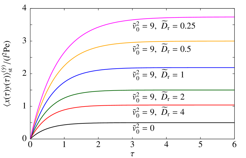
Figure 2: Rescaled response, given by Eq. (33), of a single active particle in a harmonic potential to shear flow as a function of rescaled time $\tau$ after the flow is applied. The results are given for different values of ${\tilde{v}_{0}}^{2}$ and $\widetilde{D}_{\rm r}$ (the case ${\tilde{v}_{0}}^{2}=0$ corresponds to a passive particle).

In order to visualize Eq. (32), we rewrite it in terms of dimensionless parameters: $\tau\equiv\mu_{\rm t}kt$ (describing time in units of the relaxation time $\frac{1}{\mu_{\rm t}k}$ of the trap), ${\rm Pe}\equiv\frac{\dot{\gamma}}{\mu_{\rm t}k}$ (Péclet number), $\widetilde{D}_{\rm r}\equiv\frac{D_{\rm r}}{\mu_{\rm t}k}$ (normalizing rotational relaxation time $D_{\rm r}^{-1}$ by the relaxation time $\frac{1}{\mu_{\rm t}k}$ of the trap), ${\tilde{v}_{0}}^{2}\equiv\frac{v_{0}^{2}}{D_{\rm t}\mu_{\rm t}k}$ (comparing swim speed to translational diffusion and the strength of the trap). Rescaling ${\langle x(t)y(t)\rangle}_{\rm st}^{(\dot{\gamma})}$ by the unit of squared length, $l^{2}\equiv\frac{D_{\rm t}}{\mu_{\rm t}k}$, and dividing by ${\rm Pe}$, we rewrite Eq. (32) as

$$\frac{{\langle x(\tau)y(\tau)\rangle}_{\rm st}^{(\dot{\gamma})}}{l^{2}{\rm Pe}}=\frac{1}{2}\left(1-e^{-2\tau}\right)+\frac{{\tilde{v}_{0}}^{2}}{4\left({\widetilde{D}_{\rm r}}^{2}-1\right)}$$

$$\times\Bigg{\{}\widetilde{D}_{\rm r}\left(1-e^{-2\tau}\right)-\frac{2}{\widetilde{D}_{\rm r}+1}\left(1-e^{-\left(\widetilde{D}_{\rm r}+1\right)\tau}\right)\Bigg{\}}.$$ (33)

This function is plotted in Figure 2 as a function of $\tau$ for different values of ${\tilde{v}_{0}}^{2}$ and $\widetilde{D}_{\rm r}$, thereby summarizing the above discussions. One can see in Fig. 2 that the response increases as $\widetilde{D}_{\rm r}$ decreases, because the active motion becomes more persistent.

V Numerical Example: Interacting particles in two space dimensions

The potential utility of Eq. (21) lies in its application to experiments and computer simulations of interacting particles, which we address in this section. We demonstrate this numerically for a two-dimensional system of particles trapped in a harmonic potential $U^{\rm ext}=\frac{k}{2}\sum_{i=1}^{N}(x_{i}^{2}+y_{i}^{2})$, and interacting with a short-ranged harmonic repulsion, $U_{ij}^{\rm int}(r_{ij})=\frac{k^{\rm int}}{2}(r_{c}-r_{ij})^{2}$ for $r_{ij}<r_{c}$ (where $r_{ij}$ is the distance between particle $i$ and particle $j\neq i$) and $U_{ij}^{\rm int}=0$ otherwise. A similar scenario has been studied in Ref. [34] for passive particles.

We take the radius of interaction $r_{c}=1$ as our space unit, and choose $k=1$ and the mobility $\mu_{\rm t}=1$, thus fixing the time and energy scales. The dynamics, Eq. (1), is integrated using Euler time-stepping.

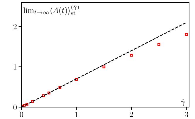
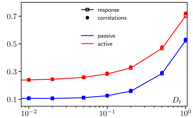
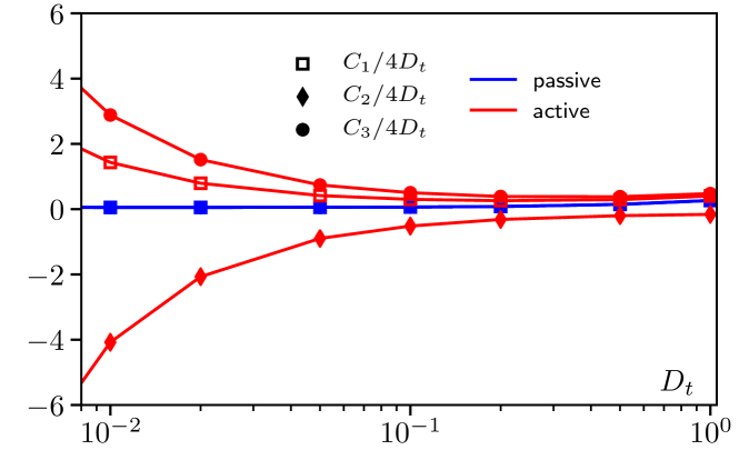
Figure 3: Numerical results for a suspension of interacting active particles ($M_{i}=0$). Top: Response measured in the sheared system for active particles with $D_{\rm t}=1$. The dashed black line is a fit in the linear regime at small $\dot{\gamma}$. Center: Comparison of the response and correlations, i.e., the left-hand and right-hand sides of Eq. (34), respectively. Bottom: Detail of each term on the right-hand side of Eq. (34). Parameters: $N=10$ particles, $k=1$, $k^{\rm int}=0.5$, $\mu_{\rm t}=1$, and $v_{0}=D_{\rm r}=\mu_{\rm r}=1$ for active particles. Time step $dt=0.02$.

We measure independently the two sides of Eq. (21) for $A(t)=\sum_{i=1}^{N}x_{i}(t)y_{i}(t)$ in steady state ($t\to\infty$) which characterizes the distortion of the density distribution due to the shear flow, and which is identified with $\sigma_{xy}^{\rm ext}$ in Eq. (16), $A(t)=\sum_{i=1}^{N}x_{i}(t)y_{i}(t)=\sigma_{xy}^{\rm ext}$. The boundary term ${\left\langle A(t)\sum_{i=1}^{N}x_{i}(0)y_{i}(0)\right\rangle}_{\rm st}$ in Eq. (21) is then irrelevant. It is illustrative to split Eq. (21) into its different contributions,

$$\frac{{\langle A(t)\rangle}_{\rm st}^{(\dot{\gamma})}-{\langle A\rangle}_{\rm st}}{\dot{\gamma}}=\frac{C_{1}+C_{2}+C_{3}}{4D_{\rm t}},$$ (34)

where

$$C_{1}={\left\langle A(t)\sum_{i=1}^{N}x_{i}(t)y_{i}(t)\right\rangle}_{\rm st},$$ (35a)

$$C_{2}=-2v_{0}\int_{0}^{t}dt^{\prime}{\left\langle A(t)\sum_{i=1}^{N}\cos\varphi_{i}(t^{\prime})y_{i}(t^{\prime})\right\rangle}_{\rm st},$$ (35b)

$$C_{3}=2\mu_{\rm t}\int_{0}^{t}dt^{\prime}{\left\langle A(t)\left[\sigma^{\rm int}_{xy}(t^{\prime})-\sum_{i=1}^{N}F_{ix}^{\rm ext}y_{i}(t^{\prime})\right]\right\rangle}_{\rm st}.$$ (35c)

As in the previous section, due to the isotropicity of the unsheared system, ${\langle A\rangle}_{\rm st}=0$.

The results obtained for $N=10$ particles interacting with a spring constant $k^{\rm int}=0.5$ for various $D_{\rm t}$ are shown in Fig. 3 for both active (with $v_{0}=D_{\rm r}=\mu_{\rm r}=1$) and passive ($v_{0}=0$) particles. The response is first obtained by simulating the sheared system at different shear rates and extracting the small $\dot{\gamma}$ behavior as shown in Fig. 3 (top). In Fig. 3 (center) we then compare to the right-hand side of Eq. (34), obtained by measuring the appropriate correlation functions in the unperturbed system. We find the two measurements to agree perfectly, given the numerical uncertainty.

First, Fig. 3 (center) shows that the response is positive and is increased by activity, as was observed for a single particle in the previous section. Second, it is interesting to compare the limits $D_{\rm t}\to 0$ in the passive and active cases because they show qualitatively different behaviors. In the passive case, this corresponds to the zero-temperature limit so that the system becomes frozen in a minimal energy configuration. We find numerically that both $C_{1}$ and $C_{3}$ in Eqs. (35a) and (35c) are proportional to $D_{\rm t}$ in this limit ($C_{2}$ vanishes for passive particles). As a result, the two terms $\frac{C_{1}}{4D_{\rm t}}$ and $\frac{C_{3}}{4D_{\rm t}}$ become constant at small $D_{\rm t}$, as shown in Fig. 3 (bottom). In contrast, active particles are still moving even at $D_{\rm t}=0$ so that the correlators $C_{i}$ do not vanish. As a result, each of the terms on the right-hand side of Eq. (34) diverges when $D_{\rm t}\to 0$ in such a way that the sum remains constant. While confirming the applicability of Eq. (21) to many-body systems, this analysis also highlights a limitation of our formulation. Indeed, our derivation necessitates a finite $D_{\rm t}$, since the distributional description of particle trajectories relies on the presence of stochasticity. However, $D_{\rm t}$ is often negligible in active systems, since the particles’ motion in that case is primarily due to activity [50, 51, 67]. It may thus be desirable to obtain formulas valid for $D_{\rm t}=0$, as is done in Ref. [49] for a different active particle model.

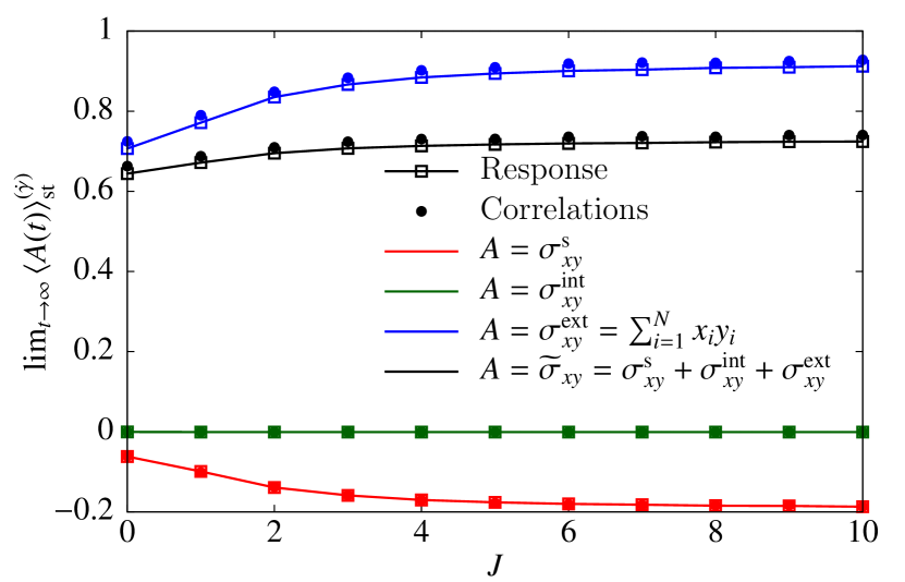
Figure 4: Numerical results for a suspension of interacting active particles subject to alignment interactions given in Eq. (36), as a function of strength of alignment $J$. Shown is the response of the terms appearing in the pseudostress tensor $\widetilde{\sigma}_{xy}$ defined in Eq. (16): the swim stress tensor $\sigma^{\rm s}_{xy}$, the conventional interaction stress tensor $\sigma_{xy}^{\rm int}$, and the external stress tensor $\sigma^{\rm ext}_{xy}$. The latter equals the observable studied in Fig. 3, i.e., $\sigma^{\rm ext}_{xy}=\sum_{i=1}^{N}x_{i}y_{i}$. Parameters as in Fig. 3 and $D_{\rm t}=1$.

Next, we include alignment interactions modeled by torques

$$M_{i}=-J\sum_{j=1(j\neq i)}^{N}\sin(\varphi_{i}-\varphi_{j}),$$ (36)

where the sum runs over particles in contact, i.e., with the interparticle distance $r_{ij}<r_{c}$. This torque arises from a typical “spin”-interaction, formed by scalar products of particle orientation vectors $\hat{\mathbf{u}}_{i}$, and is hence symmetric under interchange of $x$ and $y$ coordinates. Formula (21) can therefore be applied.

Additionally to $\sigma_{xy}^{\rm ext}$, we compute also $\sigma_{xy}^{\rm int}$ and $\sigma_{xy}^{\rm s}$ defined in Eq. (16). The results are given in Fig. 4. First, we note that the magnitudes of all stress tensor components increase with the alignment. We may expect that strong alignment renders the particle cloud into an elongated shape, which is more susceptible to shear. The saturation for large values of $J$ is expected, as, once all velocities are perfectly aligned, increasing $J$ has no effect. Notably, the interaction stress $\sigma_{xy}^{\rm int}$ remains zero within errors. While this appears plausible, in the sense that the external force balances the shear force in Eq. (1), we are not aware of a proof that $\sigma_{xy}^{\rm int}=0$ exactly.

VI Conclusion

In this paper, we have studied the linear response to simple shear flow of interacting active Brownian particles with external forces. The path integral formalism yields, in two space dimensions, the linear response formula (13) relating any time dependent state observable of the sheared system to correlation functions of the unsheared system.

For systems and observables obeying $xy$ symmetry, the initial response formula was shown to simplify such that the final result, Eq. (25), contains only state variables and is valid in any space dimension and for a wider set of activity models. This simplification is a consequence of the fact that shear in the $x$ direction and shear in the $y$ direction, having opposite torques, are equivalent for $xy$ symmetric systems and observables. This form of the response formula is particularly advantageous since it involves quantities that are typically easier to measure.

Next, we investigated the morphology and stresses of a two-dimensional cluster formed by $N$ interacting active particles confined by a harmonic potential under shear. Performing analytical computations for $N=1$ and numerical simulations for $N>1$ particles, we found that the average of $\sum_{i=1}^{N}x_{i}y_{i}$ under shear is nonnegative and larger compared to passive particles. We also found that increasing the persistence of active particles (decreasing $D_{\rm r}$) or adding alignment interactions between the particles increases the response to shear, so that the magnitudes of the found stresses increase.

Future work may consider the limit of zero translational diffusion, as well as the viscosity of a suspension of active Brownian particles. Finally, the extension to higher order responses is also a promising avenue to explore, since this could, for example, shed light on the coupling between shear translation and shear rotation.

Appendix A Detailed computation of the response in Subsec. IV.2

This Appendix sets out the necessary steps to compute all terms of Eq. (31) explicitly.

A.1 Computation of the left-hand side of Eq. (31)

First, one can show that

$${\langle\cos\varphi(s_{1})\cos\varphi(s_{2})\rangle}_{\rm st}^{(\dot{\gamma})}={\langle\sin\varphi(s_{1})\sin\varphi(s_{2})\rangle}_{\rm st}^{(\dot{\gamma})}=\frac{1}{2}\cos\left\{\frac{\dot{\gamma}}{2}\left[s_{1}-s_{2}\right]\right\}e^{-D_{\rm r}|s_{1}-s_{2}|}$$ (37)

and

$${\langle\cos\varphi(s_{1})\sin\varphi(s_{2})\rangle}_{\rm st}^{(\dot{\gamma})}=\frac{1}{2}\sin\left\{\frac{\dot{\gamma}}{2}\left[s_{1}-s_{2}\right]\right\}e^{-D_{\rm r}|s_{1}-s_{2}|},$$ (38)

in agreement with Ref. [48]. For the unsheared correlators, we hence have

$${\langle\cos\varphi(s_{1})\cos\varphi(s_{2})\rangle}_{\rm st}={\langle\sin\varphi(s_{1})\sin\varphi(s_{2})\rangle}_{\rm st}=\frac{1}{2}e^{-D_{\rm r}|s_{1}-s_{2}|}$$ (39)

and

$${\langle\cos\varphi(s_{1})\sin\varphi(s_{2})\rangle}_{\rm st}=0.$$ (40)

Results (37) – (40) do not depend on the initial angle $\varphi(-\infty)$, because we consider stationary correlation functions, i.e., we let the angle to evolve from far away in the past [$-\infty$ limit in Eq. (30c)] such that the initial angle is forgotten. We note that this limit does not commute with the limit $D_{\rm r}\to 0$. This is physical, because for times smaller than $\frac{1}{D_{\rm r}}$ a particle remembers its initial orientation.

Due to Eq. (40),

$${\langle xy\rangle}_{\rm st}=0,$$ (41)

as in the case of a trapped passive particle. This result is intuitive, because the unsheared system is $xy$ symmetric and the particle moves around the origin. For ${\langle x(t)y(t)\rangle}_{\rm st}^{(\dot{\gamma})}$ linear in $\dot{\gamma}$, the relevant nonzero correlators are those given by Eqs. (37) and (38) linear in $\dot{\gamma}$ and $\langle f_{y}(s_{1})f_{y}(s_{2})\rangle=\frac{2D_{\rm t}}{\mu_{\rm t}^{2}}\delta(s_{1}-s_{2})$. The contribution of correlator (38) is, however, zero due to the symmetry of time integrals containing it. Multiplying solutions (30a) and (30b), inserting the above mentioned correlators, and performing the integrals, one obtains result (32).

A.2 Computation of the right-hand side of Eq. (31)

For the right-hand side of Eq. (31), we need the following correlation functions: ${\langle x(t)y(t)x(t^{\prime})y(t^{\prime})\rangle}_{\rm st}$ and ${\langle x(t)y(t)\cos\varphi(t^{\prime})y(t^{\prime})\rangle}_{\rm st}$, where $t\geq t^{\prime}$. For ${\langle x(t)y(t)x(t^{\prime})y(t^{\prime})\rangle}_{\rm st}$, the relevant nonzero correlators are those given by Eq. (39), $\langle f_{x}(s_{1})f_{x}(s_{2})\rangle=\langle f_{y}(s_{1})f_{y}(s_{2})\rangle=\frac{2D_{\rm t}}{\mu_{\rm t}^{2}}\delta(s_{1}-s_{2})$, and

$${\langle\cos\varphi(s_{1})\sin\varphi(s_{2})\cos\varphi(s_{3})\sin\varphi(s_{4})\rangle}_{\rm st}=\frac{1}{8}\exp\Big{\{}-D_{\rm r}\big{[}s_{1}+s_{2}+s_{3}+s_{4}+2\min(s_{1},s_{2})-2\min(s_{1},s_{3})$$

$$-2\min(s_{1},s_{4})-2\min(s_{2},s_{3})-2\min(s_{2},s_{4})+2\min(s_{3},s_{4})\big{]}\Big{\}}+\frac{1}{8}\exp\Big{\{}-D_{\rm r}\big{[}s_{1}+s_{2}+s_{3}+s_{4}-2\min(s_{1},s_{2})$$

$$-2\min(s_{1},s_{3})+2\min(s_{1},s_{4})+2\min(s_{2},s_{3})-2\min(s_{2},s_{4})-2\min(s_{3},s_{4})\big{]}\Big{\}}-\frac{1}{8}\exp\Big{\{}-D_{\rm r}\big{[}s_{1}+s_{2}+s_{3}+s_{4}$$

$$-2\min(s_{1},s_{2})+2\min(s_{1},s_{3})-2\min(s_{1},s_{4})-2\min(s_{2},s_{3})+2\min(s_{2},s_{4})-2\min(s_{3},s_{4})\big{]}\Big{\}},$$ (42)

where $\min(s_{1},s_{2})=s_{1}$ if $s_{1}<s_{2}$ and $\min(s_{1},s_{2})=s_{2}$ if $s_{2}<s_{1}$. Note that the second term in Eq. (42) equals minus the third one with either $s_{1}$ and $s_{2}$ or $s_{3}$ and $s_{4}$ interchanged. This leads to cancelation of these terms being integrated over either $s_{1}$ and $s_{2}$ or $s_{3}$ and $s_{4}$ in the same range. Therefore, these terms do not contribute to ${\langle x(t)y(t)x(t^{\prime})y(t^{\prime})\rangle}_{\rm st}$ or to ${\langle x(t)y(t)\cos\varphi(t^{\prime})y(t^{\prime})\rangle}_{\rm st}$. The final result for ${\langle x(t)y(t)x(t^{\prime})y(t^{\prime})\rangle}_{\rm st}$ reads as

$${\langle x(t)y(t)x(t^{\prime})y(t^{\prime})\rangle}_{\rm st}=\frac{D_{\rm t}^{2}}{{(\mu_{\rm t}k)}^{2}}e^{-2\mu_{\rm t}k(t-t^{\prime})}+\frac{v_{0}^{2}D_{\rm t}}{{(\mu_{\rm t}k)}^{2}\left[D_{\rm r}^{2}-{(\mu_{\rm t}k)}^{2}\right]}\left\{D_{\rm r}e^{-2\mu_{\rm t}k(t-t^{\prime})}-\mu_{\rm t}ke^{-(D_{\rm r}+\mu_{\rm t}k)(t-t^{\prime})}\right\}$$

$$+\frac{v_{0}^{4}}{8{(\mu_{\rm t}k)}^{2}\left[D_{\rm r}^{2}-{(\mu_{\rm t}k)}^{2}\right]\left[4D_{\rm r}^{2}-{(\mu_{\rm t}k)}^{2}\right]\left[3D_{\rm r}-\mu_{\rm t}k\right]\left[D_{\rm r}+3\mu_{\rm t}k\right]}\Bigg{\{}2D_{\rm r}^{2}\left[3D_{\rm r}-\mu_{\rm t}k\right]\left[4D_{\rm r}+5\mu_{\rm t}k\right]e^{-2\mu_{\rm t}k(t-t^{\prime})}$$

$$\ \ \ \ -12D_{\rm r}\mu_{\rm t}k\left[4D_{\rm r}^{2}-{(\mu_{\rm t}k)}^{2}\right]e^{-(D_{\rm r}+\mu_{\rm t}k)(t-t^{\prime})}+{(\mu_{\rm t}k)}^{2}\left[D_{\rm r}-\mu_{\rm t}k\right]\left[D_{\rm r}+3\mu_{\rm t}k\right]e^{-4D_{\rm r}(t-t^{\prime})}\Bigg{\}},$$ (43)

where the first term is the result for a passive particle, the second term results from coupling between active motion and translational diffusion, and the third term is a purely active contribution. For ${\langle x(t)y(t)\cos\varphi(t^{\prime})y(t^{\prime})\rangle}_{\rm st}$, the relevant nonzero correlators are $\langle f_{x}(s_{1})f_{x}(s_{2})\rangle=\langle f_{y}(s_{1})f_{y}(s_{2})\rangle=\frac{2D_{\rm t}}{\mu_{\rm t}^{2}}\delta(s_{1}-s_{2})$ and those given by Eqs. (39) and (42). We get

$${\langle x(t)y(t)\cos\varphi(t^{\prime})y(t^{\prime})\rangle}_{\rm st}=\frac{v_{0}D_{\rm t}}{2\mu_{\rm t}k\left[D_{\rm r}^{2}-{(\mu_{\rm t}k)}^{2}\right]}\left\{2D_{\rm r}e^{-2\mu_{\rm t}k(t-t^{\prime})}-\left(D_{\rm r}+\mu_{\rm t}k\right)e^{-(D_{\rm r}+\mu_{\rm t}k)(t-t^{\prime})}\right\}$$

$$+\frac{v_{0}^{3}}{8\mu_{\rm t}k\left[D_{\rm r}^{2}-{(\mu_{\rm t}k)}^{2}\right]\left[4D_{\rm r}^{2}-{(\mu_{\rm t}k)}^{2}\right]\left[3D_{\rm r}-\mu_{\rm t}k\right]\left[D_{\rm r}+3\mu_{\rm t}k\right]}\Bigg{\{}4D_{\rm r}^{2}\left[3D_{\rm r}-\mu_{\rm t}k\right]\left[4D_{\rm r}+5\mu_{\rm t}k\right]e^{-2\mu_{\rm t}k(t-t^{\prime})}$$

$$\ \ \ \ -6D_{\rm r}\left[4D_{\rm r}^{2}-{(\mu_{\rm t}k)}^{2}\right]\left[D_{\rm r}+3\mu_{\rm t}k\right]e^{-(D_{\rm r}+\mu_{\rm t}k)(t-t^{\prime})}+\mu_{\rm t}k\left[D_{\rm r}-\mu_{\rm t}k\right]\left[2D_{\rm r}+\mu_{\rm t}k\right]\left[D_{\rm r}+3\mu_{\rm t}k\right]e^{-4D_{\rm r}(t-t^{\prime})}\Bigg{\}}.$$ (44)

Using Eqs. (43) and (44), we find for the three terms on the right-hand side of Eq. (31)

$$\frac{\dot{\gamma}}{4D_{\rm t}}{\left\langle x(t)y(t)\left[x(t)y(t)-x(0)y(0)\right]\right\rangle}_{\rm st}=\frac{\dot{\gamma}D_{\rm t}}{4{(\mu_{\rm t}k)}^{2}}\left(1-e^{-2\mu_{\rm t}kt}\right)+\frac{\dot{\gamma}v_{0}^{2}}{4{(\mu_{\rm t}k)}^{2}\left[D_{\rm r}^{2}-{(\mu_{\rm t}k)}^{2}\right]}\Bigg{\{}D_{\rm r}\left(1-e^{-2\mu_{\rm t}kt}\right)$$

$$-\mu_{\rm t}k\left(1-e^{-(D_{\rm r}+\mu_{\rm t}k)t}\right)\Bigg{\}}+\frac{\dot{\gamma}v_{0}^{4}}{32D_{\rm t}{(\mu_{\rm t}k)}^{2}\left[D_{\rm r}^{2}-{(\mu_{\rm t}k)}^{2}\right]\left[4D_{\rm r}^{2}-{(\mu_{\rm t}k)}^{2}\right]\left[3D_{\rm r}-\mu_{\rm t}k\right]\left[D_{\rm r}+3\mu_{\rm t}k\right]}$$

$$\ \ \ \ \times\Bigg{\{}2D_{\rm r}^{2}\left[3D_{\rm r}-\mu_{\rm t}k\right]\left[4D_{\rm r}+5\mu_{\rm t}k\right]\left(1-e^{-2\mu_{\rm t}kt}\right)-12D_{\rm r}\mu_{\rm t}k\left[4D_{\rm r}^{2}-{(\mu_{\rm t}k)}^{2}\right]\left(1-e^{-(D_{\rm r}+\mu_{\rm t}k)t}\right)$$

$$\ \ \ \ \ \ \ \ +{(\mu_{\rm t}k)}^{2}\left[D_{\rm r}-\mu_{\rm t}k\right]\left[D_{\rm r}+3\mu_{\rm t}k\right]\left(1-e^{-4D_{\rm r}t}\right)\Bigg{\}},$$ (45)

$$-\frac{\dot{\gamma}v_{0}}{2D_{\rm t}}\int_{0}^{t}dt^{\prime}{\left\langle x(t)y(t)\cos\varphi(t^{\prime})y(t^{\prime})\right\rangle}_{\rm st}=-\frac{\dot{\gamma}v_{0}^{2}}{4{(\mu_{\rm t}k)}^{2}\left[D_{\rm r}^{2}-{(\mu_{\rm t}k)}^{2}\right]}\Bigg{\{}D_{\rm r}\left(1-e^{-2\mu_{\rm t}kt}\right)-\mu_{\rm t}k\left(1-e^{-(D_{\rm r}+\mu_{\rm t}k)t}\right)\Bigg{\}}$$

$$-\frac{\dot{\gamma}v_{0}^{4}}{16D_{\rm t}{(\mu_{\rm t}k)}^{2}\left[D_{\rm r}^{2}-{(\mu_{\rm t}k)}^{2}\right]\left[4D_{\rm r}^{2}-{(\mu_{\rm t}k)}^{2}\right]\left[3D_{\rm r}-\mu_{\rm t}k\right]\left[D_{\rm r}+3\mu_{\rm t}k\right]}$$

$$\ \ \ \ \times\Bigg{\{}2D_{\rm r}^{2}\left[3D_{\rm r}-\mu_{\rm t}k\right]\left[4D_{\rm r}+5\mu_{\rm t}k\right]\left(1-e^{-2\mu_{\rm t}kt}\right)-\frac{6D_{\rm r}\mu_{\rm t}k}{D_{\rm r}+\mu_{\rm t}k}\left[4D_{\rm r}^{2}-{(\mu_{\rm t}k)}^{2}\right]\left[D_{\rm r}+3\mu_{\rm t}k\right]\left(1-e^{-(D_{\rm r}+\mu_{\rm t}k)t}\right)$$

$$\ \ \ \ \ \ \ \ +\frac{{(\mu_{\rm t}k)}^{2}}{4D_{\rm r}}\left[D_{\rm r}-\mu_{\rm t}k\right]\left[2D_{\rm r}+\mu_{\rm t}k\right]\left[D_{\rm r}+3\mu_{\rm t}k\right]\left(1-e^{-4D_{\rm r}t}\right)\Bigg{\}},$$ (46)

$$\frac{\dot{\gamma}\mu_{\rm t}k}{2D_{\rm t}}\int_{0}^{t}dt^{\prime}{\left\langle x(t)y(t)x(t^{\prime})y(t^{\prime})\right\rangle}_{\rm st}=\frac{\dot{\gamma}D_{\rm t}}{4{(\mu_{\rm t}k)}^{2}}\left(1-e^{-2\mu_{\rm t}kt}\right)+\frac{\dot{\gamma}v_{0}^{2}}{4{(\mu_{\rm t}k)}^{2}\left[D_{\rm r}^{2}-{(\mu_{\rm t}k)}^{2}\right]}\Bigg{\{}D_{\rm r}\left(1-e^{-2\mu_{\rm t}kt}\right)$$

$$-\frac{2{(\mu_{\rm t}k)}^{2}}{D_{\rm r}+\mu_{\rm t}k}\left(1-e^{-(D_{\rm r}+\mu_{\rm t}k)t}\right)\Bigg{\}}+\frac{\dot{\gamma}v_{0}^{4}}{16D_{\rm t}{(\mu_{\rm t}k)^{2}}\left[D_{\rm r}^{2}-{(\mu_{\rm t}k)}^{2}\right]\left[4D_{\rm r}^{2}-{(\mu_{\rm t}k)}^{2}\right]\left[3D_{\rm r}-\mu_{\rm t}k\right]\left[D_{\rm r}+3\mu_{\rm t}k\right]}$$

$$\times\Bigg{\{}D_{\rm r}^{2}\left[3D_{\rm r}-\mu_{\rm t}k\right]\left[4D_{\rm r}+5\mu_{\rm t}k\right]\left(1-e^{-2\mu_{\rm t}kt}\right)-\frac{12D_{\rm r}{(\mu_{\rm t}k)}^{2}}{D_{\rm r}+\mu_{\rm t}k}\left[4D_{\rm r}^{2}-{(\mu_{\rm t}k)}^{2}\right]\left(1-e^{-(D_{\rm r}+\mu_{\rm t}k)t}\right)$$

$$\ \ \ \ +\frac{{(\mu_{\rm t}k)}^{3}}{4D_{\rm r}}\left[D_{\rm r}-\mu_{\rm t}k\right]\left[D_{\rm r}+3\mu_{\rm t}k\right]\left(1-e^{-4D_{\rm r}t}\right)\Bigg{\}}.$$ (47)

Adding the right-hand sides of Eqs. (45) – (47) together, one finds that the terms proportional to $\frac{\dot{\gamma}v_{0}^{4}}{D_{\rm t}{(\mu_{\rm t}k)}^{2}}$ cancel and the rest gives Eq. (32). This completes our check of Eq. (31).

In addition, we also checked that ${\langle x(t)y(t)\cos\varphi(t^{\prime})y(t^{\prime})\rangle}_{\rm st}={\langle x(t)y(t)\sin\varphi(t^{\prime})x(t^{\prime})\rangle}_{\rm st}$, thereby confirming, for this specific example, our statement in Subsec. III.4 regarding the fact that the terms $\cos\varphi_{i}(t^{\prime})y_{i}(t^{\prime})$ and $\sin\varphi_{i}(t^{\prime})x_{i}(t^{\prime})$ in Eq. (20) give identical contributions.

References

- Vicsek et al. [1995] T. Vicsek, A. Czirók, E. Ben-Jacob, I. Cohen, and O. Shochet, Phys. Rev. Lett. 75, 1226 (1995).
- Ballerini et al. [2008] M. Ballerini, N. Cabibbo, R. Candelier, A. Cavagna, E. Cisbani, I. Giardina, V. Lecomte, A. Orlandi, G. Parisi, A. Procaccini, M. Viale, and V. Zdravkovic, Proc. Natl. Acad. Sci. USA 105, 1232 (2008).
- Dombrowski et al. [2004] C. Dombrowski, L. Cisneros, S. Chatkaew, R. E. Goldstein, and J. O. Kessler, Phys. Rev. Lett. 93, 098103 (2004).
- Sokolov et al. [2007] A. Sokolov, I. S. Aranson, J. O. Kessler, and R. E. Goldstein, Phys. Rev. Lett. 98, 158102 (2007).
- Marchetti et al. [2013] M. C. Marchetti, J. F. Joanny, S. Ramaswamy, T. B. Liverpool, J. Prost, M. Rao, and R. A. Simha, Rev. Mod. Phys. 85, 1143 (2013).
- Zöttl and Stark [2016] A. Zöttl and H. Stark, J. Phys.: Condens. Matter 28, 253001 (2016).
- Bechinger et al. [2016] C. Bechinger, R. Di Leonardo, H. Löwen, C. Reichhardt, G. Volpe, and G. Volpe, Rev. Mod. Phys. 88, 045006 (2016).
- Dhont [1996] J. K. G. Dhont, An Introduction to Dynamics of Colloids (Elsevier Science, Amsterdam, 1996).
- Larson [1999] R. Larson, The Structure and Rheology of Complex Fluids, Vol. 702 (Oxford University Press, New York, 1999).
- Rafaï et al. [2010] S. Rafaï, L. Jibuti, and P. Peyla, Phys. Rev. Lett. 104, 098102 (2010).
- Sokolov and Aranson [2009] A. Sokolov and I. S. Aranson, Phys. Rev. Lett. 103, 148101 (2009).
- López et al. [2015] H. M. López, J. Gachelin, C. Douarche, H. Auradou, and E. Clément, Phys. Rev. Lett. 115, 028301 (2015).
- Horner et al. [2018] J. S. Horner, M. J. Armstrong, N. J. Wagner, and A. N. Beris, J. Rheol. 62, 577 (2018).
- Hatwalne et al. [2004] Y. Hatwalne, S. Ramaswamy, M. Rao, and R. A. Simha, Phys. Rev. Lett. 92, 118101 (2004).
- Takatori and Brady [2017] S. C. Takatori and J. F. Brady, Phys. Rev. Lett. 118, 018003 (2017).
- Saintillan [2010] D. Saintillan, Exp. Mech. 50, 1275 (2010).
- Fielding et al. [2011] S. M. Fielding, D. Marenduzzo, and M. E. Cates, Phys. Rev. E 83, 041910 (2011).
- Callen and Welton [1951] H. B. Callen and T. A. Welton, Phys. Rev. 83, 34 (1951).
- Weber [1956] J. Weber, Phys. Rev. 101, 1620 (1956).
- Kubo [1966] R. Kubo, Rep. Prog. Phys. 29, 255 (1966).
- Green [1954] M. S. Green, J. Chem. Phys. 22, 398 (1954).
- Kubo et al. [1991] R. Kubo, M. Toda, and N. Hashitsume, Statistical Physics II: Nonequilibrium Statistical Mechanics, 2nd ed. (Springer, Berlin, 1991).
- Harada and Sasa [2005] T. Harada and S.-i. Sasa, Phys. Rev. Lett. 95, 130602 (2005).
- Speck and Seifert [2006] T. Speck and U. Seifert, Europhys. Lett. 74, 391 (2006).
- Blickle et al. [2007] V. Blickle, T. Speck, C. Lutz, U. Seifert, and C. Bechinger, Phys. Rev. Lett. 98, 210601 (2007).
- Chetrite et al. [2008] R. Chetrite, G. Falkovich, and K. Gawedzki, J. Stat. Mech.: Theor. Exp. 2008, P08005 (2008).
- Baiesi et al. [2009a] M. Baiesi, C. Maes, and B. Wynants, Phys. Rev. Lett. 103, 010602 (2009a).
- Baiesi et al. [2009b] M. Baiesi, C. Maes, and B. Wynants, J. Stat. Phys. 137, 1094 (2009b).
- Baiesi et al. [2010] M. Baiesi, E. Boksenbojm, C. Maes, and B. Wynants, J. Stat. Phys. 139, 492 (2010).
- Prost et al. [2009] J. Prost, J.-F. Joanny, and J. M. R. Parrondo, Phys. Rev. Lett. 103, 090601 (2009).
- Krüger and Fuchs [2009] M. Krüger and M. Fuchs, Phys. Rev. Lett. 102, 135701 (2009).
- Seifert [2010] U. Seifert, Phys. Rev. Lett. 104, 138101 (2010).
- Seifert [2012] U. Seifert, Rep. Prog. Phys. 75, 126001 (2012).
- Warren and Allen [2012] P. B. Warren and R. J. Allen, Phys. Rev. Lett. 109, 250601 (2012).
- Caprini et al. [2018] L. Caprini, U. M. B. Marconi, and A. Vulpiani, J. Stat. Mech.: Theor. Exp. 2018, 033203 (2018).
- Fodor et al. [2016] E. Fodor, C. Nardini, M. E. Cates, J. Tailleur, P. Visco, and F. van Wijland, Phys. Rev. Lett. 117, 038103 (2016).
- Sharma and Brader [2016] A. Sharma and J. M. Brader, J. Chem. Phys. 145, 161101 (2016).
- Merlitz et al. [2018] H. Merlitz, H. D. Vuijk, J. Brader, A. Sharma, and J.-U. Sommer, J. Chem. Phys. 148, 194116 (2018).
- Fily and Marchetti [2012] Y. Fily and M. C. Marchetti, Phys. Rev. Lett. 108, 235702 (2012).
- Buttinoni et al. [2013] I. Buttinoni, J. Bialké, F. Kümmel, H. Löwen, C. Bechinger, and T. Speck, Phys. Rev. Lett. 110, 238301 (2013).
- Zöttl and Stark [2012] A. Zöttl and H. Stark, Phys. Rev. Lett. 108, 218104 (2012).
- Reddig and Stark [2013] S. Reddig and H. Stark, J. Chem. Phys. 138, 234902 (2013).
- Hu et al. [2015] J. Hu, M. Yang, G. Gompper, and R. G. Winkler, Soft Matter 11, 7867 (2015).
- Matas-Navarro et al. [2014] R. Matas-Navarro, R. Golestanian, T. B. Liverpool, and S. M. Fielding, Phys. Rev. E 90, 032304 (2014).
- Furukawa et al. [2014] A. Furukawa, D. Marenduzzo, and M. E. Cates, Phys. Rev. E 90, 022303 (2014).
- Uspal et al. [2015] W. E. Uspal, M. N. Popescu, S. Dietrich, and M. Tasinkevych, Soft Matter 11, 6613 (2015).
- ten Hagen et al. [2011] B. ten Hagen, R. Wittkowski, and H. Löwen, Phys. Rev. E 84, 031105 (2011).
- Li et al. [2017] Y. Li, F. Marchesoni, T. Debnath, and P. K. Ghosh, Phys. Rev. E 96, 062138 (2017).
- Szamel [2017] G. Szamel, Europhys. Lett. 117, 50010 (2017).
- Deseigne et al. [2010] J. Deseigne, O. Dauchot, and H. Chaté, Phys. Rev. Lett. 105, 098001 (2010).
- Ginot et al. [2015] F. Ginot, I. Theurkauff, D. Levis, C. Ybert, L. Bocquet, L. Berthier, and C. Cottin-Bizonne, Phys. Rev. X 5, 011004 (2015).
- d’Alessandro et al. [2017] J. d’Alessandro, A. P. Solon, Y. Hayakawa, C. Anjard, F. Detcheverry, J.-P. Rieu, and C. Riviere, Nat. Phys. 13, 999 (2017).
- Hennes et al. [2017] M. Hennes, J. Tailleur, G. Charron, and A. Daerr, Proc. Natl. Acad. Sci. USA 114, 5958 (2017).
- Cugliandolo and Lecomte [2017] L. F. Cugliandolo and V. Lecomte, J. Phys. A: Math. Theor. 50, 345001 (2017).
- Altland and Simons [2010] A. Altland and B. Simons, Condensed Matter Field Theory, 2nd ed. (Cambridge University Press, 2010).
- Martin et al. [1973] P. C. Martin, E. D. Siggia, and H. A. Rose, Phys. Rev. A 8, 423 (1973).
- Janssen [1976] H.-K. Janssen, Z. Phys. B: Condens. Matter 23, 377 (1976).
- De Dominicis and Peliti [1978] C. De Dominicis and L. Peliti, Phys. Rev. B 18, 353 (1978).
- Onsager and Machlup [1953] L. Onsager and S. Machlup, Phys. Rev. 91, 1505 (1953).
- Machlup and Onsager [1953] S. Machlup and L. Onsager, Phys. Rev. 91, 1512 (1953).
- Note [1] The action is generically quadratic in due to the Gaussian nature of the noise.
- Basu et al. [2015] U. Basu, M. Krüger, A. Lazarescu, and C. Maes, Phys. Chem. Chem. Phys. 17, 6653 (2015).
- Gardiner [2010] C. W. Gardiner, Handbook on Stochastic Methods (Springer, Berlin, 2010).
- Wynants [2010] B. Wynants, Structures of Nonequilibrium Fluctuations: Dissipation and Activity, Ph.D. thesis, K.U.Leuven (2010).
- Fuchs and Cates [2005] M. Fuchs and M. E. Cates, J. Phys.: Condens. Matter 17, S1681 (2005).
- Takatori et al. [2014] S. C. Takatori, W. Yan, and J. F. Brady, Phys. Rev. Lett. 113, 028103 (2014).
- Bricard et al. [2013] A. Bricard, J.-B. Caussin, N. Desreumaux, O. Dauchot, and D. Bartolo, Nature 503, 95 (2013).