Efficient and scalable data structures and algorithms for
goal-oriented adaptivity of space-time FEM codes

Abstract

The cost- and memory-efficient numerical simulation of coupled volume-based multi-physics problems like flow, transport, wave propagation and others remains a challenging task with finite element method (FEM) approaches. Goal-oriented space and time adaptive methods derived from the dual weighted residual (DWR) method appear to be a shiny key technology to generate optimal space-time meshes to minimise costs. Current implementations for challenging problems of numerical screening tools including the DWR technology broadly suffer in their extensibility to other problems, in high memory consumption or in missing system solver technologies. This work contributes to the efficient embedding of DWR space-time adaptive methods into numerical screening tools for challenging problems of physically relevance with a new approach of flexible data structures and algorithms on them, a modularised and complete implementation as well as illustrative examples to show the performance and efficiency.

1 Motivation and significance

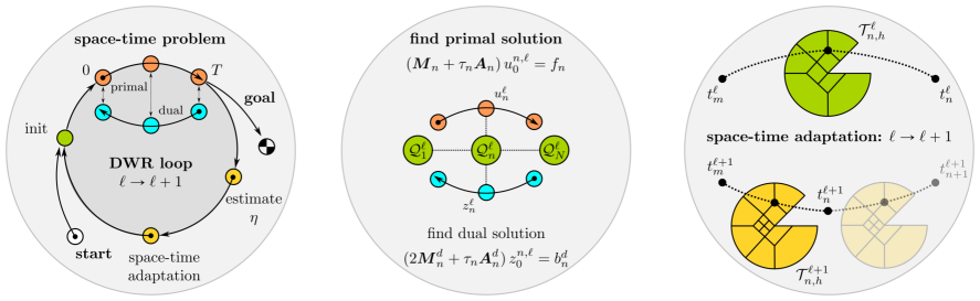
Figure 1: General workflow of the space-time adaptive numerical simulation tools DTM++.Project/dwr-* using the dual weighted residuals (DWR) technique for the error estimation (left), an exemplary forward and backward time marching step $n$ on $(d$+$1)$-dimensional space-time slabs $\mathcal{Q}_{n}^{\ell}$ in the DWR loop $\ell$ (middle) and an exemplary space-time adaptation update of the spatial triangulation $\mathcal{T}_{h,n}^{\ell}\to\mathcal{T}_{h,n}^{\ell+1}$ and the temporal subinterval $I_{n}^{\ell}\to I_{n}^{\ell+1}$ to prepare the DWR loop $\ell$+$1$ (right).

1.1 Introduction

The accurate, reliable and efficient numerical approximation of flow in heterogeneous deformable porous media include several coupled multi-physics phenomena, such as multi-phase diffusion and convection-dominated transport with underlying chemical reactions, deformation and poroelastic wave propagation as well as fluid-structure interactions in a more general sense, and is of fundamental importance in environmental, civil, energy, biomedical and many other engineering fields to yield a cost-effective numerical simulation screening tool to support the still challenging and fundamental research of understanding such multi-physics phenomena. Considerable representatives are coupled problems based on the Navier-Stokes equations for incompressible flow, the Euler equations for compressible flow, the convection-diffusion-reaction equations and the Biot-Allard equations for coupled flow with poroelastic wave propagation, which are characterised by partial differential equations of nonlinear and instationary character. Space-time finite element method (FEM) approximations offer appreciable benefits over finite difference and finite volume methods such as the flexibility with which they can accommodate discontinuities in the model, material parameters and boundary conditions as well as for a priori and a posteriori error estimation to establish optimal computational space-time grids in a self-adaptive way. The dual weighted residual (DWR) method for goal-oriented adaptivity was introduced by Becker and Rannacher ([1, 2]) and further studied; cf. [3, 4, 5, 6] and references therein. The DWR method facilitates to find optimal spatial mesh adaptations, optimal temporal mesh adaptations, as well as optimal local space-time polynomial degrees, tuning parameters and physical or numerical models, such that the overall computational costs are minimised for reaching a goal in a target quantity of interest.

A target quantity is a cost, error or energy functional $\mathcal{J}$ and depends on an user-chosen quantity of interest. Examples for a quantity of interest are the stress derived from the primal displacement variables or the drag coefficient derived from the primal fluid velocity variables of the underlying problem. The goal of the DWR method is to satisfy a guaranteed error bound in the target quantity of interest instead of satisfying a classical error bound of the primal solution variable in a standard norm.

Unfortunately, the DWR method still has challenging drawbacks compared to standard a posteriori error based adaptive methods. It needs to solve the primal or forward problem and an auxiliary dual or adjoint problem of higher approximation quality in each loop of an optimisation problem, it needs variational space-time discretisations for the primal and dual problem, which yield problems on $(d$+$1)$-dimensional domains, and there is a lack in efficient data structures, algorithms as well as (non-)linear system solver and preconditioning technologies for sophisticated problems of physical interest, which will be at least partially resolved by this work.

Fortunately, the DWR method works in general situations, in which the problem itself and the quantity of interest are of nonlinear fashion, and it does not rely on generally unknown assumptions of the initial space-time mesh. The key idea of the DWR method is to embed the given problem of finding solutions of a partial differential equation into the framework of optimal control to estimate the functional error of $\mathcal{J}(u)-\mathcal{J}(u_{\tau,h})$, derive computable a posteriori error estimates $\eta$ with an approximation of the corresponding dual solution $z$ of an auxiliary problem, execute space-time mesh (and other) adaptations based on the information given by $\eta$ and loop until the goal in the target quantity is reached as it is outlined by Fig. 1. Consider to solve the constrained optimisation problem given by

$$\mathcal{J}(u)=\min!\,,$$ (1)

for a (cost, error or energy) functional $\mathcal{J}$ depending on $u$, under the constraint of finding $u\in V$ from the variational problem

$$0=\mathcal{F}(\varphi)-\mathcal{A}(u)(\varphi)\,,\,\,\text{for all test functions }\varphi\in W\,,$$

which is set up from the partial differential equation problem in a standard way. $V$ and $W$ are corresponding variational trial and test space-time functional spaces such that primal and dual solutions exist at least locally, are unique and stable, but the latter ones can not be guaranteed for arbitrary nonlinear problems without restrictions. The calculus of variations theory associates a corresponding Lagrangian functional $\mathcal{L}$ to (1),

$$\mathcal{L}(u,z):=\mathcal{J}(u)+\mathcal{F}(z)-\mathcal{A}(u)(z)\,,$$ (2)

with $z\in W$ as a Lagrange multiplier or, equivalently, as the adjoint or dual solution variable, for the global optimisation problem (1). The primal solution $u$ is the first component of a stationary point $(u,z)$ of $\mathcal{L}$ whereas the second component yields the corresponding dual solution $z$; cf. [1, 2, 6] for details. Due to the mathematically challenging theory of even local existence of solutions in general nonlinear settings, we restrict ourselves further, without the loss of generality and the impact of our software, to a linear prototype model for instationary transport in heterogeneous porous media.

1.2 Exact Scientific Problem solved by the Software

The DTM++.Project/dwr-diffusion frontend simulation tool for the established finite element analysis library deal.II [7] yields a reference implementation of the prototype model for instationary transport in heterogeneous porous media. We consider the goal-oriented approximation of a target quantity $\mathcal{J}(u)$ subject to find $u\in V$ from the diffusion equation

$$\rho\,\partial_{t}u-\nabla\cdot(\epsilon\,\nabla u)=f\,,$$ (3)

in the space-time domain $\mathcal{Q}=\Omega\times I$ with $\Omega\subset\mathbb{R}^{d}$ (open and bounded), dimension $d=2,3$, and $I=(t_{0},T)$, $0\leq t_{0}<T<\infty$, and equipped with appropriate initial and boundary conditions

$$\begin{array}[]{r@{\,}c@{\,}l@{\,}l@{\,}l}u(\boldsymbol{x},t_{0})&=&u_{0}(\boldsymbol{x})&\text{in}&\Omega\times\{t_{0}\}\,,\\[4.30554pt] u(\boldsymbol{x},t)&=&g(\boldsymbol{x},t)&\text{on}&\Gamma_{D}\times I\,,\\[4.30554pt] \epsilon(\boldsymbol{x})\,\nabla u(\boldsymbol{x},t)\cdot\boldsymbol{n}(\boldsymbol{x})&=&h(\boldsymbol{x},t)&\text{on}&\Gamma_{N}\times I\,,\\[4.30554pt] \end{array}$$

with the partition of the boundary $\partial\Omega=\Gamma_{D}\cup\Gamma_{N}$ and $\Gamma_{D}\neq\emptyset$.

A target quantity $\mathcal{J}(u)$ of interest derived from the primal solution $u$ of (3) might represent a local pollution concentration under diffusive transport. The coefficient functions $\rho>0$ and $\epsilon>0$ are the mass density and the permeability of the medium, respectively, and the right hand side function $f:\mathcal{Q}\to\mathbb{R}$ represents volume forces acting on the interior domain $\Omega$ such as source or sink terms. In (3), the differential operators $\partial_{t}(\cdot)$, $\nabla\cdot(\cdot)=\partial_{x_{1}}(\cdot)+\dots+\partial_{x_{d}}(\cdot)$ and $\nabla(\cdot)=[\partial_{x_{1}}(\cdot),\dots,\partial_{x_{d}}(\cdot)]^{T}$ denote the partial derivative for the time variable $t$, the divergence and the gradient for the space variables $x_{1},\dots,x_{d}$, respectively, and, $\boldsymbol{n}$ denotes the outward facing normal vector, in standard notation. The initial-boundary value problem is closed by the choice of an appropriate initial value function $u_{0}:\Omega\to\mathbb{R}$ and a boundary value function $g:\Gamma_{D}\times I\to\mathbb{R}$ acting on the Dirichlet part of the boundary partition $\Gamma_{D}\neq\emptyset$. Additionally, there is the choice for an appropriate inhomogeneous Neumann boundary type condition function $h:\Gamma_{N}\times I\to\mathbb{R}$ if $\Gamma_{N}\neq\emptyset$.

The weak variational primal problem, for brevity consider to find $u:=\tilde{u}-g$ or put $g=0$ without loss of generality of the following discussion, reads as: Seek $u\in V$, $V=L^{2}(0,T;H^{1}_{0}(\Omega))$, satisfying $u(0)=u_{0}$, $u_{0}\in H^{1}_{0}(\Omega)$, such that

$$A(u)(\varphi)=F(\varphi)\,,\,\,\forall\varphi\in W=L^{2}(0,T;H^{1}_{0}(\Omega))\,,$$ (4)

with the left-hand side bilinear form $A:V\times W\to\mathbb{R}$,

$$A(u)(\varphi):=\displaystyle\int_{0}^{T}\int_{\Omega}\Big{(}\varphi\cdot\rho\,\partial_{t}u+\nabla\varphi\cdot(\epsilon\,\nabla u)\Big{)}\,\operatorname{d}\boldsymbol{x}\,\operatorname{d}t\,,$$

and the right-hand side linear form $F:W\to\mathbb{R}$,

$$F(\varphi):=\displaystyle\int_{0}^{T}\int_{\Omega}\varphi\cdot f\,\operatorname{d}\boldsymbol{x}\,\operatorname{d}t\,,\,\,f\in L^{2}(0,T;L^{2}(\Omega))\,.$$

Remark that $\tilde{u}\in g+V$, with $\tilde{u}$ having inhomogeneous Dirichlet boundary conditions $g\neq 0$, can be generated in a standard way as it will be explained in the following algorithm. Briefly, the weak variational dual problem results from the stationary condition of $\mathcal{L}(u,z)$ (2) given by

$$\Bigg{\{}\begin{array}[]{c}\mathcal{J}(u+\psi)-\mathcal{J}(u)-A(\psi)(z)\\ F(\varphi)-A(u)(\varphi)\end{array}\Bigg{\}}\stackrel{{\scriptstyle!}}{{=}}\Bigg{\{}\begin{array}[]{c}0\\ 0\end{array}\Bigg{\}}\,,$$ (5)

for $\psi\in V$ and $z\in W$; using the Euler-Lagrange method of constrained optimisation, cf. for details [6, Sec. 6.1], [4]. The dual problem for a general nonlinear goal functional $\mathcal{J}(u)$ reads as: Find $z\in W$, $W=L^{2}(0,T;H^{1}_{0}(\Omega))$, satisfying $z(T)=z_{T}$, $z_{T}\in H^{1}_{0}(\Omega)$, such that

$$A^{\ast}(z)(\psi)=\mathcal{J}(u+\psi)-\mathcal{J}(u)-\int_{\Omega}\psi(T)\cdot z(T)\,\operatorname{d}\boldsymbol{x}\,,$$ (6)

for all $\psi\in V$, $V=L^{2}(0,T;H^{1}_{0}(\Omega))$, and with the left-hand side adjoint bilinear form $A^{\ast}:W\times V\to\mathbb{R}$,

$$A^{\ast}(z)(\psi):=\displaystyle\int_{T}^{0}\int_{\Omega}\Big{(}\psi\cdot\rho\,\partial_{t}z-\nabla\psi\cdot(\epsilon\,\nabla z)\Big{)}\,\operatorname{d}\boldsymbol{x}\,\operatorname{d}t\,,$$

which is derived from integration by parts in time of $A(\psi)(z)$ of (4) and put this into the first equation of (5). Remark that the choice of trial and test functions for the dual problem here yields traces on $t_{0}$ and $T$. To estimate the functional error of $\mathcal{J}(u)-\mathcal{J}(u_{\tau,h})$ and to derive computable a posteriori error estimates $\eta$ for the space-time mesh adaptivity, we need to discretise the primal problem (4) and the dual problem (6).

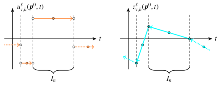
Figure 2: Exemplary illustration of fully discrete primal and dual solutions for a fixed observation point $\boldsymbol{p}^{0}\in\Omega$ in space in a DWR loop $\ell$ over time; a piecewise constant discontinuous in time primal solution $u_{\tau,h}^{\ell}(\boldsymbol{p}^{0},t)$ of (7) (left), and, a piecewise linear continuous in time dual solution $z_{\tau,h}^{\ell}(\boldsymbol{p}^{0},t)$ of (8) for a specific goal functional $\mathcal{J}(u)$ (right), and the drawn arrows represent the implemented path of the natural time integration on a ($d$+$1$)-slab approach.

The primal and dual problem are discretised with appropriate space-time variational methods, i.e. here a piecewise constant discontinuous Galerkin method in time for the primal problem and a piecewise linear continuous Petrov-Galerkin method in time for the dual problem (Fig. 2), combined with a piecewise polynomial continuous Ritz-Galerkin (FEM) method in space; cf. for details [8] and [4, 6]. The space-time cylinder $\mathcal{Q}=\Omega\times I$ is divided into non-overlapping space-time slabs $\mathcal{Q}_{n}^{\ell}=\Omega_{h}^{\ell}\times I_{n}^{\ell}$, with the partition of $\bar{I}=[t_{0},T]$ as $t_{0}=:t_{0}^{\ell}<\cdots<t_{N^{\ell}}^{\ell}:=T$, $I_{n}^{\ell}:=(t_{m}^{\ell},t_{n}^{\ell})$, $t_{m}^{\ell}:=t_{n-1}^{\ell}$, $n=1,\dots,N^{\ell}$, for the $\ell$-th loop. On each $\mathcal{Q}_{n}^{\ell}$ consider a not necessarily conforming partition $\mathcal{T}_{h,n}^{\ell}$ of $\Omega_{h}^{\ell}$ into non-overlapping elements $K_{n}^{\ell}$, denoted as geometrical quadrilaterals for $d=2$ or hexahedrons for $d=3$. The fully discrete primal and dual solutions are represented by

$$u_{\tau,h}^{\ell}(\boldsymbol{x},t)=\sum_{n=1}^{N^{\ell}}\sum_{\iota=0}^{0}\sum_{j=1}^{N_{\text{DoF}}^{\text{primal},n,\ell}}u^{n,\ell}_{j,\iota}\cdot\phi_{j}^{\text{primal},n,\ell}(\boldsymbol{x})\cdot\zeta_{\iota}^{\text{primal},n,\ell}(t)$$ (7)

$$\text{and}\quad z_{\tau,h}^{\ell}(\boldsymbol{x},t)=\sum_{n=1}^{N^{\ell}}\sum_{\iota=0}^{1}\sum_{j=1}^{N_{\text{DoF}}^{\text{dual},n,\ell}}z^{n,\ell}_{j,\iota}\cdot\phi_{j}^{\text{dual},n,\ell}(\boldsymbol{x})\cdot\xi_{\iota}^{\text{dual},n,\ell}(t)\,.$$ (8)

In (7)-(8), $u^{n,\ell}_{j,\iota}$ and $z^{n,\ell}_{j,\iota}$ denote the space-time degrees of freedom (DoF) of the primal and dual problem, $\phi_{j}^{\text{primal},n,\ell}$ and $\phi_{j}^{\text{dual},n,\ell}$ denote the global spatial trial basis functions and $\zeta_{\iota}^{\text{primal},n,\ell}$ and $\xi_{\iota}^{\text{dual},n,\ell}$ denote the global temporal trial basis functions (Fig. 3). The basis functions are defined on a reference space-time slab $\hat{\mathcal{Q}}=(0,1)^{d}\times(0,1)$, e.g. as piecewise Lagrange polynomials, and mapped appropriately to $\mathcal{T}_{h,n}^{\ell}\times I_{n}^{\ell}$; cf. [8] for details.

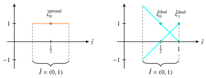
Figure 3: Illustration of temporal reference trial basis functions on the reference subinterval $\hat{I}=(0,1)$ for the primal solution (7) (left) and the dual solution (8) (right), which are mapped with $\mathcal{T}_{n}:\hat{I}\to I_{n}$, $t=\tau_{n}\cdot\hat{t}+t_{m}$, from $\hat{I}$ to $I_{n}$.

The software implements the goal functional $J:V\to\mathbb{R}$,

$$J(\psi):=\displaystyle\frac{1}{\|u-u_{\tau,h}^{\ell}\|_{\mathcal{Q}_{c}}}\,\displaystyle\int_{I_{c}}\int_{\Omega_{c}}\psi\cdot(u-u_{\tau,h}^{\ell})\,\operatorname{d}\boldsymbol{x}\,\operatorname{d}t\,,$$ (9)

for all $\psi\in V$, with $u_{\tau,h}^{\ell}$ denoting the fully discrete primal solution of the $\ell$-th DWR loop and $u$ denoting the analytic solution (only possible for academic test problems) or an approximation of the exact primal solution generated on a finer space-time mesh or with higher-order approaches, which aims to reach

$$\|u-u_{\tau,h}^{\ell}\|_{\mathcal{Q}_{c}}<\text{{tol}}\,,$$ (10)

for an absolute or relative tolerance tol criterion, on the space-time control volume $\mathcal{Q}_{c}=\Omega_{c}\times I_{c}\subseteq\mathcal{Q}$; cf. Fig. 4.

Algorithm (dwr-diffusion). Loop $\ell=1,\dots$ until the goal (10) is reached; cf. Fig. 1. Solve the primal problem: Find the coefficient vector $\boldsymbol{u}^{n,\ell}_{0}=(u^{n,\ell}_{j,0})_{j}$, $j=1,\dots,N_{\text{DoF}}^{\text{primal},n,\ell}$, from

$$(\boldsymbol{M}_{n}+\tau_{n}\,\boldsymbol{A}_{n})\,\boldsymbol{u}^{n,\ell}_{0}=\tau_{n}\,(\boldsymbol{f}^{n}_{0}+\boldsymbol{h}^{n}_{0})+\boldsymbol{M}_{n}\,(I_{h}\,u_{\tau,h}^{\ell}(\boldsymbol{x},t_{n-1}))_{j}\,,$$ (11)

for $n=1,\dots,N^{\ell}$, by marching forwardly in time through the slabs. The mass and stiffness matrix of the primal problem on the slab $n$ are denoted as $\boldsymbol{M}_{n}$ and $\boldsymbol{A}_{n}$, respectively, the right hand side assemblies $\boldsymbol{f}^{n}_{0}$ and $\boldsymbol{h}^{n}_{0}$ correspond to volume forcing and inhomogeneous Neumann boundary terms and the vector $(I_{h}\,u_{\tau,h}^{\ell}(\boldsymbol{x},t_{n-1}))_{j}$ is the interpolation of the initial value function $u_{0}$ from (3) for $n=1$ or the fully discrete primal solution of the previous ($n$-$1$) slab for $n>1$ on the primal finite element space of the current slab $\mathcal{Q}_{n}^{\ell}$. Each system is modified such that the Dirichlet boundary conditions from (3) are applied strongly. To set up the dual problem with the goal (9), compute the contribution of the value $\|u-u_{\tau,h}\|_{\mathcal{Q}_{c}}$ (10) with a post-processing on each slab $\mathcal{Q}_{n}^{\ell}$. Solve the dual problem: Find the coefficient vector $\boldsymbol{z}^{n,\ell}_{0}=(z^{n,\ell}_{j,0})_{j}$, $j=1,\dots,N_{\text{DoF}}^{\text{dual},n,\ell}$, from

$$(2\,\boldsymbol{M}_{n}^{d}+\tau_{n}\,\boldsymbol{A}_{n}^{d})\,\boldsymbol{z}^{n,\ell}_{0}=\tau_{n}\,\boldsymbol{J}^{n,\ell}_{0}+2\,\boldsymbol{M}_{n}^{d}\,(I_{h}^{d}\,z_{\tau,h}^{\ell}(\boldsymbol{x},t_{n}))_{j}\,,$$ (12)

for $n=N^{\ell},\dots,1$, by marching backwardly in time through the slabs. The mass and stiffness matrix of the dual problem on the slab $n$ are denoted as $\boldsymbol{M}_{n}^{d}$ and $\boldsymbol{A}_{n}^{d}$, respectively, the right hand side assembly vector $\boldsymbol{J}^{n,\ell}_{0}$ corresponds to the goal defined by (9) and the vector $(I_{h}^{d}\,z_{\tau,h}^{\ell}(\boldsymbol{x},t_{n}))_{j}$ is the interpolation of the homogeneous initial value function $z_{T}=0$ (6) for the chosen goal (9) for $n=N^{\ell}$ or the fully discrete dual solution of the next ($n$+$1$) slab for $n<N^{\ell}$ on the dual finite element space of the current slab $\mathcal{Q}_{n}^{\ell}$. The same type of boundary colorisation (either Dirichlet or Neumann type) is used for the dual problem but with homogeneous boundary value functions, even in the case of inhomogeneous primal boundary conditions. Each system is modified such that homogeneous Dirichlet boundary conditions on $\Gamma_{D}$ are applied strongly to the dual solution $z_{\tau,h}^{\ell}$ (8). The numerically approximated a posteriori space-time error estimate

$$\tilde{\eta}_{\tau,h}^{\ell}=\sum_{n=1}^{N^{\ell}}\tilde{\eta}^{n,\ell}\,,\quad\text{with}\quad\tilde{\eta}^{n,\ell}=\sum_{K\in\mathcal{T}_{h,n}^{\ell}}|\tilde{\eta}_{K}^{n,\ell}|\,,$$ (13)

is derived from the primal and dual solutions $u_{\tau,h}^{\ell}$ and $z_{\tau,h}^{\ell}$, respectively, and each localised $\tilde{\eta}_{K}^{n,\ell}$, $K\in\mathcal{T}_{h,n}^{\ell}$, $n=1,\dots,N^{\ell}$, is stored independently; cf. for details [5]. The space-time mesh refinement update is implemented as follows: mark a space-time slab for refinement in time for which the corresponding value of $\tilde{\eta}^{n,\ell}$ (13) belongs to the top fraction $0\leq\theta_{\tau}\leq 1$ of largest values, then, on each slab $\mathcal{Q}_{n}^{\ell}$, mark a mesh cell $K\in\mathcal{T}_{h,n}^{\ell}$ for $d$-dimensional isotropic refinement in space for which the corresponding value of $|\tilde{\eta}_{K}^{n,\ell}|$ (13) belongs to the top fraction $\theta_{h,1}$ or $\theta_{h,2}$, for a slab that is not or is marked for time refinement, of largest values, with $0\leq\theta_{h,2}\leq\theta_{h,1}\leq 1$, then execute the spatial refinement and finally execute the temporal refinement.

Figure 4: Illustration of the implemented local ($d$+$1$)-dimensional space-time control volume $\mathcal{Q}_{c}(t)=\Omega_{c}(t)\times I_{c}\subseteq\mathcal{Q}=\Omega\times I$, with $I_{c}=(t_{m,c},t_{n,c})$ and $t_{0}\leq t_{m,c}<t_{n,c}\leq T$, for Eq. (9) and Sec. 3.

1.3 Contribution of the Software to Scientific Discovery

Modules of the DTM++.Project, including higher-order in time discretisations with sophisticated solver technologies and distributed-memory parallel implementations, already have contributed to the process of scientific discovery for acoustic, elastic and coupled wave propagation (xwave), mass conservative transport (meat) and coupled deformation with transport (biot) for instance; cf. [8, 9] and references therein. The stationary predecessor of dwr-diffusion is used in [4] and the successor is used in [5] for stabilised instationary convection-dominated transport problems. The contributed software shares the modularity and flexibility of all DTM++.Project modules, it provides a freely available open-source framework for efficiently solving problems with goal-oriented adaptivity and will support further scientific discovery with numerical simulations of challenging problems with physical relevance.

1.4 Basic Setup and Usage of the Software

The user needs to prepare a deal.II v9.0 toolchain to compile and run the software, this can be done on any major platform by using candi; open a terminal and type in

it clone https://ithub.com/dealii/candi

d andi & ./candi.sh

and follow the instructions. Then download, compile and run

it clone https://ithub.org/dtm-project/dwr-diffusion

d dwr-diffusion && make . & make release

/dwr-diffusion /input/KoecherBruchhaeuser2d.prm

with the experimental setting given in Sec. 3.

1.5 Related work

The origin of the code is related to the step-14 tutorial code of deal.II [7] for the Laplace equation and other DTM++.Project modules [8]. Additionally, the code gallery of [7] provides some implementations for stationary elastoplasticity problems using DWR-based goal-oriented mesh adaptivity and for the instationary convection-diffusion-reaction equation without adaptivity for instance. All of the listed related implementations can gain advantages from our work since those are mostly specific implementations with partly lacking documentation and, more importantly, do not document their data structures and algorithms in an application-free way for allowing the reuse in other frameworks straight forwardly.

2 Software description

The software DTM++.Project/dwr-diffusion implements the introduced algorithm of Sec. 1.2 in an object-oriented way and is shipped with an extensive in-source documentation. DTM++ modules are written in the C++.17 language and make use of the new language features since C++.11 such as reference counted dynamic memory allocation, range-based loops, the auto specifier, strongly typed enum classes and others.

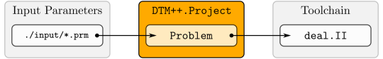
Figure 5: Pictorial DTM++.Project software module architecture overview.

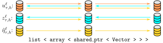
Figure 6: Pictorial overview of the DTM++.Project data storage management. A list entry corresponds to a slab and stores a small array of shared pointer references. The large data Vector is stored independently and can be serialised.

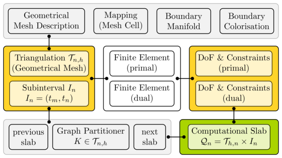
Figure 7: Pictorial overview of the elements to handle a computational slab $\mathcal{Q}_{n}=\mathcal{T}_{h,n}\times I_{n}$ implemented by the DTM++::Grid_DWR class. Remark that loop based slab data structures $\mathcal{Q}_{n}^{\ell}$ is not stored for efficiency reasons.

2.1 Software Architecture

The general workflow to use the dwr-diffusion solver module is illustrated by Fig. 5, it highly rely on user-driven inputs by simple text-based parameter input files for a wide range of similar numerical examples. To keep the code clean for the intended user group, the implementation of the presented algorithm from Sec. 1.2 is done with a procedural-structured single central solver class template Diffusion_DWR<dim> : DTM::Problem for slightly different time discretisations of the primal and dual problem. All assemblers, such as for the matrices, right-hand side vectors and even the space-time error estimate $\tilde{\eta}$, are using the deal.II workstream technology for thread-parallel and further MPI+X-parallel simulations. Thereby, the useful and efficient auxiliary classes of the DTM++ suite are provided independently, such that the input parameter handling and data output handling must not be included into the solver class. An overview on the general DTM++ software framework for PDE solver frameworks can be found in [8] and by the in-source doxygen documentation of the code.

2.2 Software Key Technologies

One of the key technologies of this work is the efficient handling of the space-time DoF data storage management as given in Fig. 6 which allow to efficiently iterate forwardly and backwardly to compute the primal and dual solutions as well as the error estimate. Another important key technology is a list approach of the new DTM++::Grid_DWR class to handle ($d$+$1$)-dimensional space-time computational slabs and grids as given in Fig. 7 and allows for inexpensive local time refinements.

3 Illustrative Examples

To demonstrate the functionalities, an analytic solution $u$, which mimics a rotating cone with a time-dependent height,

$$\begin{array}[]{l@{\,}c@{\,}l}u(\boldsymbol{x},t)&:=&u_{1}\cdot u_{2}\,,\,\,\boldsymbol{x}=[x_{1},x_{2}]\in\mathbb{R}^{2}\text{ and }t\in\mathbb{R}\,,\\[2.15277pt] u_{1}(\boldsymbol{x},t)&:=&(1+a\cdot((x_{1}-m_{1}(t))^{2}+(x_{2}-m_{2}(t))^{2}))^{-1}\,,\\[2.15277pt] u_{2}(t)&:=&\nu_{1}(t)\cdot s\cdot\arctan(\nu_{2}(t))\,,\end{array}$$ (14)

with $m_{1}(t):=\frac{1}{2}+\frac{1}{4}\cos(2\pi t)$ and $m_{2}(t):=\frac{1}{2}+\frac{1}{4}\sin(2\pi t)$, and, $\nu_{1}(\hat{t}):=-1$, $\nu_{2}(\hat{t}):=5\pi\cdot(4\hat{t}-1)$, for $\hat{t}\in[0,0.5)$ and $\nu_{1}(\hat{t}):=1$, $\nu_{2}(\hat{t}):=5\pi\cdot(4(\hat{t}-0.5)-1)$, for $\hat{t}\in[0.5,1)$, $\hat{t}=t-k$, $k\in\mathbb{N}_{0}$, and, scalars $a,s\in\mathbb{R}$, $a>0$, is approximated on a two-dimensional L-shaped domain (Fig. 4) for $I=(0,1.25)$ with the minimisation goal from (9) on a time-dependent space-time control volume $\mathcal{Q}_{c,\text{KB2d}}=\Omega_{c}(t)\times I_{c}$, with $\Omega_{c}(t)=\{{\boldsymbol{x}\in\mathbb{R}^{2}}\,|\,\boldsymbol{x}-[0.5,0.5]^{T}=\hat{\boldsymbol{x}}+\boldsymbol{m}(t;r_{1})\,,\,\hat{\boldsymbol{x}}\in\hat{\Omega}\,,\,\boldsymbol{m}(t;r_{1})=r_{1}\cdot[\cos(t),\,\sin(t)]^{T}\}$, $\hat{\Omega}=(\hat{p}^{1}_{1},\,\hat{p}^{2}_{1})\times(\hat{p}^{1}_{2},\,\hat{p}^{2}_{2})\subset\mathbb{R}^{2}$ and $I_{c}=(0.25,1)$.

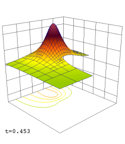
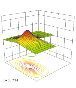
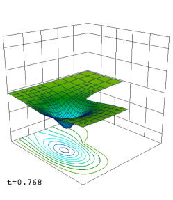
Figure 8: Solution profiles $u_{\tau,h}^{18}$ and dual solution $z_{\tau,h}^{18}$ contour lines for Sec. 3.

The setup uses $\Omega_{h}=\{(0,1)^{2}\}\setminus\{(0.5,1)^{2}\}$, $\Gamma_{N}=\{\boldsymbol{x}\in\bar{\Omega}_{h}\,|\,x_{1}=0\}$, $\Gamma_{D}=\partial\bar{\Omega}_{h}\setminus\Gamma_{N}$. The functions $u_{0}$, $f$, $g$ and $h$ of (3) are derived from the analytic solution (14), the coefficient functions are set to $\rho=0.8$ and $\epsilon=1.2$, and, the scalars are set to $a=50$ and $s=-0.3333$. The space-time triangulation for $\ell=1$ is composed of $N^{1}=5$ slabs having 3 spatial cells each. The goal tolerance is $\text{{tol}}=10^{-2}\cdot\|u-u_{\tau,h}^{1}\|_{\mathcal{Q}_{c}}$. Solution profiles for $u_{\tau,h}$ and contour lines of $z_{\tau,h}$ are illustrated in Fig. 8. Selected convergence and error estimator results as well as a quality measurement $I_{\text{eff}}:=|\tilde{\eta}_{\tau,h}^{\ell}/(J(u)-J(u_{\tau,h}^{\ell}))|$, where $I_{\text{eff}}=1$ is optimal, are given by Tab. 1.

$\ell$	$N^{\ell}$	$|\mathcal{T}_{h,\star}^{\ell}|$	$\|u-u_{\tau,h}^{\ell}\|_{\mathcal{Q}_{c}}$	$\tilde{\eta}_{\tau,h}^{\ell}$	I${}_{\text{eff}}$
1	5	3	6.070e-02	1.994e-02	0.33
2	6	12	2.634e-02	2.451e-02	0.93
$\cdots$			$\cdots$
17	227	441	7.304e-04	2.030e-04	0.28
18	295	603	5.744e-04	1.723e-04	0.30

Table 1: Selected convergence and error estimator results of loop $\ell$, having $N^{\ell}$ slabs and the max. number of mesh cells $|\mathcal{T}_{h,\star}^{\ell}|$ on a slab $n=\star$, for Sec. 3.

By Fig. 9 the distribution of the time subinterval lengths of $\mathcal{Q}_{n}^{\ell}$ over $I$ are illustrated. The goal (10) is reached for the 18th loop of the optimisation problem (Tab. 1) with an absolute error $\|u-u_{\tau,h}^{18}\|_{\mathcal{Q}_{c}}=5.744\cdot 10^{-4}$.

The numerical results (Fig. 8-9) highlight the local space-time refinement characteristic of the solver in a self-adaptive way, while the finer space-time cells are located inside and close to the boundary of the control volume $\mathcal{Q}_{c,\text{KB2d}}(\boldsymbol{x},t)$, $t\in(0.25,1)$. Remark that not any refinement is done for $t>1$ of this parabolic problem since the control volume is not active.

4 Impact

The software gives new and efficient insights to the implementation of goal-oriented mesh adaptivity which supports the development of cost-effective numerical screening tools based on finite element approaches for fundamental problems in science and engineering. Derivatives of the software have already been used for stabilised stationary and instationary convection-dominated problems with goal-oriented mesh adaptivity in [4, 5] as well as for coupled deformation and diffusion-driven transport in [9, 8]. The intended user group of researchers and engineers using and developing finite element based numerical simulation screening tools for several problems is widespread and globally distributed; an example would be the extension of the work [10] in which they are using higher order variational time discretisations for convection-dominated transport with non-goal oriented adaptive time step control, or, an efficient instationary extension to the approach presented in [3]. The software is currently not used in commercial settings, but the license allows for the integration into commercial tools.

Figure 9: Distribution of $\tau_{n}$ of the space-time slabs $\mathcal{Q}_{n}^{\ell}$, $\ell\in\{17,18\}$, for Sec. 3.

5 Conclusions

This original software publication provides efficient and scalable data structures and algorithms for the implementation of goal-oriented mesh adaptivity in a highly modular way. The key ideas of the data structures and algorithms can be reused, even independently of the programming language, in any adaptive finite element code. The performance and applicability of the software is shown with an illustrative example and several others are shipped with the code. The work yields a major breakthrough as a freely available open-source implementation with extensive in-source documentation for the dual weighted residual method in an application-free way such that it can be easily adopted by other frameworks. Ongoing work is on the distributed-memory parallelisation, on the serialisation of the data storage hiding memory operations, and on finding optimal tuning parameters of the minimisation problem.

Required Metadata

Current code version

Ancillary data table required for subversion of the codebase. Kindly replace examples in right column with the correct information about your current code, and leave the left column as it is.

Nr.	Code metadata description	Please fill in this column
C1	Current code version	Version 1.0.0
C2	Permanent link to code/repository used for this code version	https://github.com/ dtm-project/dwr-diffusion
C3	Legal Code License	https://github.com/ dtm-project/dwr-diffusion/License
C4	Code versioning system used	git
C5	Software code languages, tools, and services used	C++.17; cmake, gcc, mpi, optional: paraview, doxygen
C6	Compilation requirements, operating environments & dependencies	deal.II with hdf5; Linux (Fedora, CentOS 7, RHEL 7, etc.), MacOS, Windows WSL
C7	If available Link to developer documentation/manual	https://github.com/ dtm-project/dwr-diffusion
C8	Support email for questions	dtmproject@uwe.koecher.cc

Table 2: Code metadata (mandatory)