Low-order model for successive bifurcations of the fluidic pinball
Abstract
We propose the first least-order Galerkin model of an incompressible flow undergoing two successive supercritical bifurcations of Hopf and pitchfork type. A key enabler is a mean-field consideration exploiting the symmetry of the mean flow and the asymmetry of the fluctuation. These symmetries generalize mean-field theory, e.g. no assumption of slow growth-rate is needed. The resulting 5-dimensional Galerkin model successfully describes the phenomenogram of the fluidic pinball, a two-dimensional wake flow around a cluster of three equidistantly spaced cylinders. The corresponding transition scenario is shown to undergo two successive supercritical bifurcations, namely a Hopf and a pitchfork bifurcations on the way to chaos. The generalized mean-field Galerkin methodology may be employed to describe other transition scenarios.
1 Introduction
This study advances mean-field modeling for successive symmetry breaking due to Hopf and pitchfork bifurcations. The theoretical framework is applied to the transition of the flow around a cluster of circular cylinders, termed the fluidic pinball for the possibility to control fluid particle by cylinder rotation (Noack & Morzyński, 2017; Ishar et al., 2019).
Mean-field theory was pioneered by Landau (1944) and Stuart (1958) and is a singular triumph of nonlinear reduced-order modeling in fluid mechanics. Already the most simple mean-field model for the supercritical Hopf bifurcation reveals deep insights into the coupling between the fluctuations and the mean flow, e.g. the damping mechanism of unstable modes by Reynolds stress. In addition, Malkus (1956) principle of marginal stability for time-averaged flows, the square root growth law of fluctuation level with increasing Reynolds number, the cubic damping term from a linear-quadratic dynamics, the energetic explanation of this amplitude dynamics, and the slaving principle leading to manifolds driven by ensemble-averaged Reynolds stress are easily derived. Also, the idea of center manifold theory and the surprising success of linear parameter-varying models are analytically illustrated. Historically, Landau was the first to derive the normal form of the dynamics with Krylov-Bogoliubov approximation (an averaging method for spiral phase paths, see e.g. Jordan & Smith, 1999) while Stuart could explain how the cubic damping term arises from the distorted mean flow.
Mean-field models for a supercritical Hopf bifurcation with an unstable oscillatory eigenmode have been applied and validated for numerous configurations. The onset of vortex shedding behind a cylinder wake has been thoroughly investigated (Strykowski & Sreenivasan, 1990; Schumm et al., 1994; Noack et al., 2003). Even high-Reynolds number turbulent wake flow can display a distinct mean-field manifold and modeled by a noise-driven mean-field model (Bourgeois et al., 2013).
A supercritical pitchfork bifurcation similarly arises by an unstable eigenmode with a real eigenvalue. The onset of convection rolls in the Rayleigh-Bénard problem is a famous example (Zaitsev & Shliomis, 1971; Swift & Hohenberg, 1977; Cross & Hohenberg, 1993). The features of a pitchfork bifurcation are observed for the sidewise symmetry breaking of the time-averaged Ahmed body wake (Grandemange et al., 2012, 2013; Cadot et al., 2015; Bonnavion & Cadot, 2018) and more generally in three-dimensional wake flows (Mittal, 1999; Gumowski et al., 2008; Szaltys et al., 2012; Grandemange et al., 2014; Rigas et al., 2014). In contrast, the drag crisis of circular cylinder is associated with a subcritical bifurcation into two asymmetric sheddings with opposite mean lift values (Schewe, 1983).
Not surprisingly, numerous generalizations of mean-field models have been proposed. Landau (1944) and Hopf (1948) have conjectured that high-dimensional fully developed turbulence may be explained by an increasingly rapid succession of Hopf bifurcations. This idea has been discarded as unlikely (see, for instance, Landau & Lifshitz, 1987). The seminal paper by Ruelle & Takens (1971) showed that turbulence does not arise as a successive superposition of oscillators, but irregular chaotic behavior can already appear after few bifurcations. A second direction is the explanation of nonlinear coupling between two incommensurable shedding frequencies (Luchtenburg et al., 2009), also referred to as frequency crosstalk in the following. This amplitude coupling over the mean flow has been termed quasi-laminar in Reynolds & Hussain (1972) pioneering theoretical foundation of the triple decomposition. The advancements also include subcritical bifurcations (Watson, 1960). More specifically, the case of a codimension two bifurcation, involving both a pitchfork and a Hopf bifurcation, was addressed in Meliga et al. (2009), who derived the amplitude equation based on the weakly nonlinear analysis of the wake of a disk. Fabre et al. (2008) derived the same equation solely based on symmetry arguments for the wake of axisymmetric bodies. A resolvent analysis follows mean-field considerations in decomposing the flow in a time-resolved linear dynamics and a feedback-term with the quadratic nonlinearity (Gomez et al., 2016; Rigas et al., 2017).
Our study develops a generalized mean-field Galerkin model for the first two bifurcations of the fluidic pinball with increasing Reynolds number. The primary supercritical bifurcation leads to the periodic vortex shedding which is statistically symmetric. At higher Reynolds numbers, the resulting limit cycle undergoes a pitchfork bifurcation into a stable, asymmetric, mirror-symmetric pair of periodic solutions. This local bifurcation has a transverse effect resulting from the decoupling of these two bifurcations (see appendix E), which simultaneously leads to an identical local pitchfork bifurcation of the steady solution, into an unstable, asymmetric, mirror-symmetric pair of steady solutions. The underlying dynamics is modeled with a small number of assumptions. The key simplification results from exploiting the symmetry of the mean flow and the antisymmetry of the fluctuation. The generalized mean-field Galerkin methodology can be expected to be useful for describing other transition scenarios.
The manuscript is organized as follows. In § 2, the numerical plant is introduced and the Reynolds-number dependent flow behavior described. This phenomenology drives the mean-field modeling of the first two bifurcations in § 3. The resulting models for the Hopf and subsequent pitchfork bifurcation are present in § 4 and § 5, respectively. § 6 summarizes the results and outline future directions of research.
2 Flow configuration
In this section we describe the numerical toolkit and the flow features as the Reynolds number is increased. The direct Navier-Stokes solver with MATLAB interfaces, used for the simulation, is described in § 2.1. The fluidic pinball configuration and the flow features and route to chaos are described in § 2.2 and § 2.3, respectively.
2.1 Direct Navier-Stokes solver
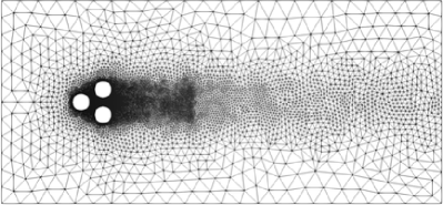
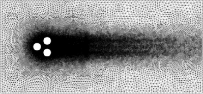
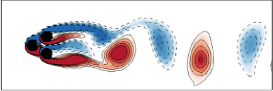
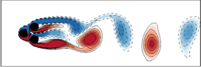
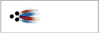
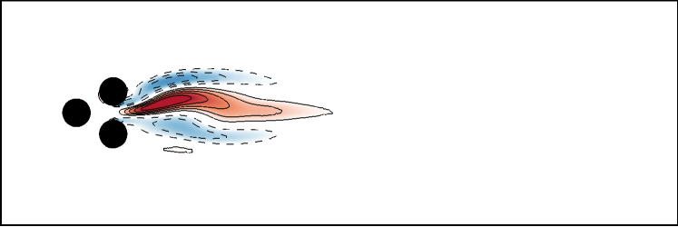
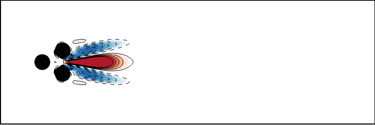
The unsteady Navier-Stokes solver is based on fully implicit time integration and Finite-Element Method discretization (Noack & Morzyński, 2017; Noack et al., 2003, 2016). The time integration is third-order accurate while FEM discretization employs a second–order Taylor-Hood finite elements (Taylor & Hood, 1973). The solution is obtained iteratively, with the Newton-Raphson type approach. The tangent matrix is updated on each iteration and computations are carried out until the residual is under a prescribed tolerance. The steady solution is obtained in a similar Newton-Raphson iteration for the steady Navier-Stokes equations. The convergence to one of the three steady solutions with different states of the base-bleeding jet is triggered by appropriate “initial” conditions in the iteration, see appendix A. The solver quickly converges to one of the steady states and a final, near-zero residual confirms that this is indeed the steady flow solution sought. The computational domain is discretized on an unstructured grid. Pinball configuration uses a grid with 4225 triangles and 8633 vertices (see figure 1(a)). To test the grid dependency of the solution we increased the number of triangles by nearly a factor 4 (26849 elements and 54195 nodes, see figure 1(b)). The flow patterns shown in figure 2 develop from a steady solution at subjected to an instantaneous rotation of cylinders at . The upper cylinder rotates counterclockwise, the lower one clockwise and the center cylinder also in a clockwise direction — all with unit circumferential velocity, i.e. the velocity of oncoming flow . This configuration and boundary conditions result in a vortex shedding shown in figure 2 for the time instance . Both simulations prove grid independence and yield dynamically consistent results (see figure 2).
| (a) | (b) |
|---|---|
 |
 |
| (a) | (b) |
|---|---|
 |
 |
2.2 Pinball configuration
We refer to the configuration shown in figure 1 as the fluidic pinball as the rotation speeds allow one to change the paths of the incoming fluid just as flippers manipulate the ball of a conventional pinball machine. The fluidic pinball is a set of three equal circular cylinders with radius placed parallel to each other in a viscous incompressible uniform flow at speed . The flow over a cluster of three parallel cylinders has been experimentally studied involving heat transfer, fluid-structure interactions and multiple frequencies interactions over the past few decades (Price & Paidoussis, 1984; Sayers, 1987; Lam & Cheung, 1988; Tatsuno et al., 1998; Bansal & Yarusevych, 2017). For the fluidic pinball, the cylinders can rotate at different speeds creating a kaleidoscope of vortical structures or variety of steady flow solutions. The configuration is used for evaluation of flow controllers (Cornejo Maceda, 2017) as this problem is a challenging task for control methods comprising several frequency crosstalk mechanisms (Noack & Morzyński, 2017). The centers of the cylinders form an equilateral triangle with side length , symmetrically positioned with respect to the flow. The leftmost triangle vertex points upstream, while the rightmost side is orthogonal to the oncoming flow. The origin of the Cartesian coordinate system is placed in the middle of the top and bottom cylinder. The fluidic pinball computational domain, shown in figure 1 is bounded by the rectangle .
Without forcing, the boundary conditions comprise a no-slip condition on the cylinders and a unit velocity in the far field:
| (1) |
The far field boundary conditions are exerted on the inflow, upper and lower boundaries while the outflow boundary is assumed to be a stress–free one, transparent for the outgoing fluid structures. A typical initial condition is the unstable steady Navier-Stokes solution .
In this study, all three cylinders remain static as we are interested in the natural dynamics of the flow as the Reynolds number is increased.
2.3 Flow features
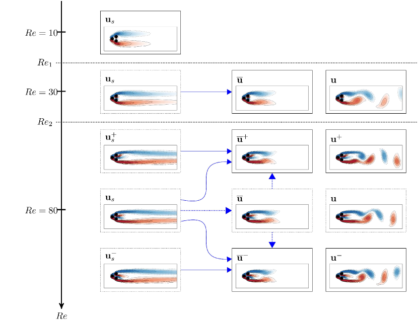
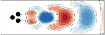
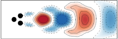
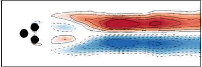
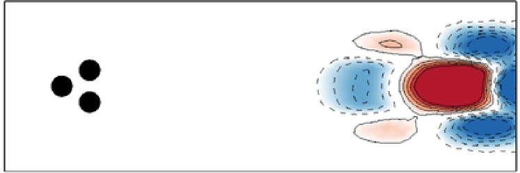
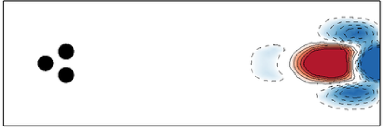
The steady solution , shown in figure 3 for different values of the Reynolds number , is stable up to the critical value . This value corresponds to with respect to the actual body height , which is consistent with the critical value of the Reynolds number found for a single cylinder (Ding & Kawahara, 1999; Barkley, 2006). Beyond , the steady solution becomes unstable with respect to vortices periodically and alternately shed at the top and bottom of the two right-most cylinders, following a Hopf bifurcation (instability of the fixed point via a pair of complex-conjugated eigenvalues, see e.g. Strogatz et al. (1994)). In addition to the resulting von Kármán street of vortices, the gap between the cylinders makes possible the formation of a jet at the base of the two outer cylinders. The steady solution , the mean flow and the instantaneous flow field , are shown in figure 3, for .
The flow passing between the two rearward cylinders, the base-bleeding flow, has a critical impact on the successive bifurcations undergone by the system on the route to chaos. Indeed, beyond a secondary critical value of the Reynolds number, the system undergoes a pitchfork bifurcation, which affects both the fixed point or the limit cycle, via a real eigenvalue, see e.g. Strogatz et al. (1994). As a result, the symmetry of both the steady solution and the mean flow is broken with respect to the symmetry plane defined by . This is illustrated by the two mirror-conjugated steady solutions and the two associated mean flows , shown in figure 3 for , where the base-bleeding jet appears deflected to either upward or downward with respect to the symmetry plane. Note, however, that a symmetry-preserving mean flow ( in figure 3 for ) still exists beyond the secondary bifurcation, so that three mean flows exist beyond : two of them, , are mirror-conjugated and break the symmetry, while the last one, preserves the symmetry. This bifurcation of the limit cycle is coincident with the bifurcation of the fixed point, as three steady solutions can be found beyond : are mirror-conjugated and break the symmetry, while the last one, preserves the symmetry. Yet, all three of them are unstable with respect to the cyclic shedding of von Kármán vortices, in which symmetry properties of the steady solution are succeeded in the resulting mean flow. When the initial condition is close to the symmetric steady solution , the flow regime arrives after a long transient on a limit cycle whose mean flow is symmetric, as illustrated in figure 3 for . However, the dynamics of this limit cycle is only transient, indicating that it is not a stable state. After a new transient, depending on the details of the initial condition, the flow regime eventually reaches one of the two mirror-conjugated limit cycles (centered on either ). When the initial condition already breaks the symmetry of the flow configuration, the unstable “symmetry-centered” limit cycle is not explored and the system reaches directly one of the two stable limit cycles. The transient dynamics between these six typical states beyond illustrate a transverse action on the original state space resulting from the new active symmetric breaking mode decoupling with the primary Hopf bifurcation, as detailed in appendix D. The new active degree of freedom introduced by the pitchfork instability is responsible for the two simultaneous local pitchfork bifurcations, of both the steady solution and the periodic solution, as shown in the appendices B and C. The simultaneous bifurcation of the steady and periodic solution has also been observed for the cylinder wake transition from stability analyses (Noack & Eckelmann, 1994a, b) and from 3D Navier-Stokes simulations (Zhang et al., 1994). A further discussion about this non-generic situation is recorded in appendix E. Besides, the linear stability analysis (see appendix B) and the Floquet stability analysis (see appendix C) around have been performed to prove these two simultaneous bifurcations.
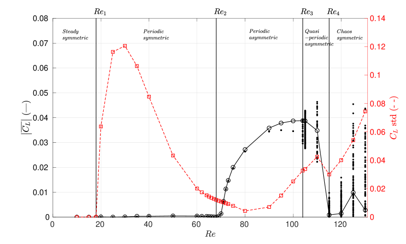
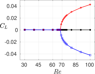
As a result, when the symmetry of vortex shedding is broken, the mean value (solid line) of the pressure lift coefficient , where is the total lift force from pressure, no longer vanishes, as shown in figure 4. At the precision of our investigation, both the Hopf and pitchfork bifurcations were found to be supercritical.
The fluctuation amplitude of the lift coefficient is minimum for , as shown in figure 4 (dashed curve). It starts to decrease around , when the jet starts to grow at the base of the two outer cylinders. Henceforth, the growth of the base-bleeding jet, as the Reynolds number is increased, seems to be fed with the energy of the fluctuations. Transfers of energy between the dynamically dominant degrees of freedom will be made clear in § 3.
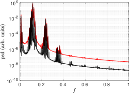
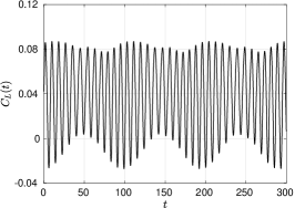
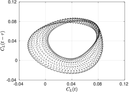
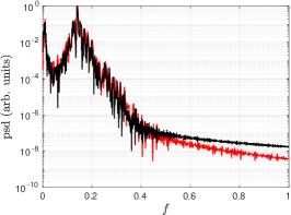
When the Reynolds number is further increased up to a critical value , a new frequency rises in the power spectrum of the lift coefficient . This frequency is about one order of magnitude smaller than the natural frequency of the vortex shedding, as illustrated in figure 5(a) for and in the movie QP.MP4 of the additional materials. The low and natural frequencies couple to generate combs of sharp peaks in the power spectrum, while the background level depends on the length of the time series. The new frequency is associated with modulations of the base-bleeding jet around its deflected position. A visual inspection of both the time series and the phase portrait at indicates that the new frequency also modulates the amplitude (figure 5(b)) of the main oscillator and thickens the limit cycle associated with the main oscillator (figure 5(c)). All these features are typical of a quasi-periodic dynamics, indicating that the system has most likely undergone a Neimark-Säcker bifurcation, e.g. a secondary Hopf bifurcation, at , after which two mirror-conjugated 2-tori exist in the state space of the system.
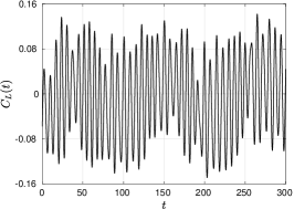
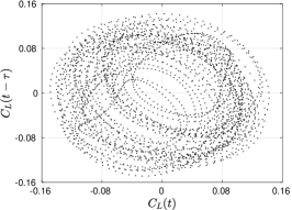
At even larger values of the Reynolds number, , the main peak in the power spectral density of the lift coefficient widens significantly, as shown in figure 6(a) for . In this new regime, the instantaneous flow field is characterized by random switches between an upward or downward base-bleeding jet, see the movie CHAOS.MP4 in the additional materials, and the mean flow is symmetric, as shown in figure 4 for . The time series exhibits neither periodic nor quasi-periodic features anymore (see figure 6(b)) and the phase portrait exhibits a much more complex dynamics (see figure 6(c)). The dynamical regime henceforth exhibits many features of a chaotic regime, indicating that the system has most likely followed the Ruelle-Takens-Newhouse route to chaos (Newhouse et al., 1978).
| (a) | (b) | (c) |
|---|---|---|
 |
 |
 |
| (a) | (b) | (c) |
|---|---|---|
 |
 |
 |
3 Low-dimensional modeling
We derive a mean-field Galerkin model for the primary and secondary bifurcations of the fluidic pinball. First (§ 3.1), the Galerkin method is recapitulated as a very general approach to reduced-order models. In § 3.2, the constitutive equations of the mean-field model are derived from a minimal set of assumptions. Then, mean-field Galerkin models are derived for the Hopf bifurcation (§ 3.3), the pitchfork bifurcation (§ 3.4) and the succession of both bifurcations (§ 3.5).
3.1 Galerkin method
The starting point is the non-dimensionalized incompressible Navier-Stokes equations:
| (2) |
where . The velocity field satisfies the no-slip condition on the cylinders, the free-stream condition at the inflow, a no-slip condition at the top and bottom boundary and the no-stress condition at the outflow. The steady solution satisfies the steady Navier-Stokes equations:
| (3) |
The Galerkin method is based on an inner product in the space of square-integrable vector fields in the observation domain . The standard inner product between and reads:
| (4) |
A traditional Galerkin approximation with a basic mode , for instance, the steady solution and orthonormal expansion modes , with time-dependent amplitudes , reads:
| (5) |
Orthonormality implies:
| (6) |
The projection of (5) on (2) leads to the linear-quadratic Galerkin system (Fletcher, 1984),
| (7) |
Following Rempfer & Fasel (1994), is introduced. The coefficients and parametrize the viscous and convective Navier-Stokes terms. The pressure term vanishes for sufficiently large domains and is neglected in the following.
In the following, the steady solution is taken as the basic mode . This implies that is a fixed point of (7) and the constant term vanishes as the projection of onto the th mode . In this case, (7) can be re-written as a linear-quadratic system of ordinary differential equations :
| (8) |
where and for .
3.2 Mean-field modeling
Mean-field modeling allows a dramatic simplification of a general Galerkin system (8) close to bifurcations. In this section, we derive constitutive equations with a small number of more general assumptions.
In the spirit of the Reynolds decomposition, the velocity field is decomposed into a slowly varying distorted mean flow and fluctuation with first-order (relaxational) or second-order (oscillatory) dynamics:
| (9) |
Here, the mean-field deformation is the difference between the distorted mean flow and the steady solution. For the oscillatory dynamics considered, the distorted mean flow can be defined as an average over one local fluctuation period denoted by . Thus,
| (10) |
After the pitchfork bifurcation into two mirror-conjugated flows , , a symmetric distorted mean flow is enforced via
| (11) |
We note that is not the mean flow, which is defined by the post-transient limit
| (12) |
The distorted mean flow coincides with mean flow for the post-transient phase before the pitchfork bifurcation. Technically, a harmonic fluctuation is assumed and this one period average is computed as an average of all phases in . The somewhat loaded term “distorted mean flow” is directly adopted from the original publications of mean-field theory (Stuart, 1958). J.T. Stuart considers this flow as “distorted” from the steady solution by the Reynolds stress associated with the instability mode(s).
For a nominally symmetric cylindrical obstacle, the distorted mean flow can be expected to be symmetric while the dominant fluctuation is antisymmetric. This leads to a symmetry-based decomposition of the flow into a symmetric contribution with
| (13) |
and an antisymmetric component satisfying
| (14) |
Here, and denote the set of symmetric and antisymmetric vector fields, respectively. The resulting decomposition reads
| (15) |
In the sequel, we will identify the distorted mean flow with the symmetric component and the fluctuation with the antisymmetric one:
| (16) |
This identification is justified for symmetry-breaking bifurcations with first- or second-order dynamics with neglected higher harmonics. For brevity, and are introduced as symmetric and antisymmetric subsets of .
The convective term is easily shown to have the following symmetry properties:
| (17a) | |||||
| (17b) | |||||
| (17c) | |||||
| (17d) | |||||
The antisymmetric component is derived starting with (2), subtracting the steady version of (3) and exploiting the symmetry of , the antisymmetry of as well as the symmetry relations (17). The fluctuation dynamics reads:
| (18) |
Analogously, the symmetric part describes the distorted mean flow dynamics:
| (19) |
Note that this symmetric component of the Navier-Stokes equations has not yet been averaged and the sum of Eqs. (3), (19) and (18) leads to the Navier-Stokes equations (2). To this point, all equations are strict identities for the symmetric and antisymmetric part of the Navier-Stokes dynamics.
Next, we follow mean-field arguments and consider and as small perturbations around the fixed point . Let and where and are smallness parameters. Hence, can be neglected in comparison to the terms , . We follow Stuart’s original idea to separate between the fluctuation driven by the instability and the resulting mean-field deformation and arrive at the unsteady linearized Reynolds equation,
| (20) |
The mean-field deformation characterized by the scale is seen to respond linearly to the Reynolds stress force scaling with . Hence, .
Summarizing, Eqs. (18) and (20) are the constitutive equations of mean-field theory exploiting only symmetry and smallness of the mean-field deformation.
Close to the critical Reynolds number , the temporal growth rate can be Taylor expanded to and can be assumed to be small. In this case, , i.e. the time derivative of (20) can be neglected with respect to the other terms . This leads to the steady linearized Reynolds equation:
| (21) |
This equation is also true for the post-transient solution, e.g. the limit cycle of a Hopf bifurcation or the asymmetric state of a pitchfork bifurcation. Often, the distorted mean flow quickly responds to the Reynolds stress even far away from the bifurcation.
3.3 Supercritical Hopf bifurcation
At low Reynolds numbers, a symmetric stable steady solution is observed. Periodic vortex shedding sets in with the occurrence of an unstable oscillatory antisymmetric eigenmode at . The Reynolds-number dependent initial growth rate and frequency are denoted by and , respectively. The real and imaginary parts of this eigenmode are and , respectively, both antisymmetric modes. In the following, these modes are assumed to be orthonormalized.
This oscillation generates a Reynolds stress, which changes the mean flow via (20). The mean flow deformation is described by the symmetric shift mode with unit norm. By symmetry, the first two modes are orthogonal with respect to the shift mode. Thus, the modes form an orthonormal basis. The resulting Galerkin expansion reads:
| (22) |
Moreover, polar coordinates are introduced , , where and are assumed to be slowly varying functions of time.
Substituting (22) in (18), projecting on , and applying the Krylov-Bogoliubov (Jordan & Smith, 1999) averaging method yields:
| (23a) | |||||
| (23b) | |||||
Here, for a supercritical Hopf bifurcation. We refer to Noack et al. (2003) for details.
Krylov-Bogoliubov averaging implies a harmonic balancing on the slowly varying amplitude and frequency of oscillatory and the slowly varying dynamics. The corresponding original theorem includes a convergence proof of this approximation for a second-order ordinary differential equation for oscillations in the limit of small nonlinearity. We cannot perform this limit but justify the operation on the a priori observation that quadratic Galerkin system terms are typically two orders of magnitude smaller than the dominant linear coefficients, i.e. describe a small nonlinearity. A posteriori the operation is justified by the results, i.e. by obtaining amplitudes and frequencies with up to a few percent error.
Substituting (22) in (21) replaces (25) by the mean-field manifold:
| (24) |
with derivable proportionality constant .
Alternatively, the mean-field manifold may be obtained from the Galerkin system. Substituting (22) in (20) and projecting on yields:
| (25) |
where and are necessary for a globally stable limit cycle. Note that (25) can be rewritten as:
| (26) |
Now, the slaving process which leads to the mean-field manifold of (24) can be appreciated from the mean-field Galerkin system. If , the timescale of slaving to the fluctuation level is much smaller than the timescale of the transient and can be set to zero.
Eqs. (23) and (24) yield the famous Landau equations with the cubic damping term:
| (27) |
The Landau oscillator leads to a stable limit cycle with , frequency and shift-mode amplitude . The three nonlinearity parameters , and can be uniquely derived from the limit cycle parameters , , and . The growth rate needs to be chosen sufficiently large, e.g. to ensure slaving on the manifold.
Eqs. (23), (25) are the mean-field Galerkin system, while Eqs. (23), (24) characterize the original mean-field model, i.e. the slaved Galerkin system. Near the Hopf bifurcation, when crosses the zero line at , the growth rate is approximated by implying the square-root law .
The Landau equation has been proposed by Landau (see, e.g. Landau & Lifshitz, 1987), derived from the Navier-Stokes equation by Stuart (1958), generalized for Galerkin systems by Noack et al. (2003), and validated in numerous simulations and experiments for cylinder wakes (Schumm et al., 1994) and other soft onsets of oscillatory flows. We note that the proposed derivation from symmetry considerations constrains the model to symmetric obstacles but liberates the mean-field Galerkin model from typical assumptions, likes closeness to the Hopf bifurcation or the need for frequency filtered Navier-Stokes equations.
3.4 Supercritical pitchfork bifurcation
![[Uncaptioned image]](/html/1812.08529/assets/x13.png)
Next, the symmetry-breaking pitchfork bifurcation of a steady symmetric Navier-Stokes equation is considered. Now, mode describes the antisymmetric instability with positive growth rate . The shift mode prevents unbounded exponential growth. The corresponding Galerkin expansion reads
| (28) |
Substituting (28) in Eqs. (18) and (20), and exploiting the symmetry of the modes, yields:
| (29a) | |||||
| (29b) | |||||
Note that a linear term and quadratic and terms in (29a) are ruled out by symmetry. Similarly, a linear term or a mixed quadratic term in (29b) are prohibited by symmetry. The quadratic term is not consistent with the linearized Reynolds equation (20). The pitchfork bifurcation can be considered as a Hopf bifurcation with and a single mode. Replacing by , by and setting yields (29a) from (23) and (29b) from (25)—modulo names of the coefficients.
Eqs. (29a), (29b) are the mean-field Galerkin system. Substituting (28) in (21) yields the manifold:
| (30) |
with . The asymmetric steady solutions read , . The two nonlinearity parameters , are readily determined from the two asymptotic values and . The growth rate can be set in analogy to the previous model to to ensure slaving on the manifold.
From (29a) and (30), the famous unstable dynamics with cubic damping term is obtained:
where for a supercritical bifurcation. Eqs. (29a), (29b) are the mean-field Galerkin system.
Near the secondary pitchfork bifurcation, and . The parameters of the pitchfork Galerkin system can be derived from the eigenmode and the asymptotic state in complete analogy to § 3.3. The growth rate will ensure the slaving of (30). We emphasize that this pitchfork model is derived primarily from symmetry considerations and does not require closeness to the critical parameter.
3.5 Pitchfork bifurcation of periodic solution
In the final modeling effort, a low-dimensional model from a primary supercritical Hopf bifurcation at and a secondary supercritical pitchfork bifurcation at is derived following the numerical observations of the fluidic pinball in § 2. For simplicity, closeness to the secondary bifurcation is assumed. For the same reason, the mean-field Galerkin system shall still describe the periodic solution. In this case, the generalized 5-mode mean-field expansion:
| (31) |
describes the flow where and and , , being smallness parameters associated with the pitchfork bifurcation. We project Eqs. (18) and (20) on (31). The terms encapsulate the original Hopf model while the low-pass filtered terms yield the original pitchfork system. This yields the following generalized mean-field system:
| (32a) | |||||
| (32b) | |||||
| (32c) | |||||
| (32d) | |||||
| (32e) | |||||
The linear instability parameters , , are obtained from the corresponding global stability analysis. Slaving is ensured with and . The nonlinearity parameters , , , and are determined from the limit cycle parameters , and and pitchfork parameters and in the asymptotic regime.
As the amplitude of the pitchfork bifurcation grows, the smallness argument does not hold and we get cross-terms, like . We shall not pause to elaborate on the possible generalizations now, but will return to the topic in the result section.
3.6 Sparse Galerkin model from mean-field considerations
The mean-field Galerkin system (32) with decoupled Hopf and pitchfork dynamics can, by construction, only be expected to hold near the pitchfork bifurcation . At higher Reynolds numbers , cross-terms will appear, e.g., the growth rate may also depend on the pitchfork-related shift mode amplitude . The most general Galerkin system (8) contains linear terms and quadratic terms.
The assumed symmetry of the modes excludes roughly half of these 100 coefficients. Let for symmetric mean flow modes , and for the antisymmetric fluctuation modes , . The linear coefficients
can be shown to vanish if . In other words, the coefficients vanish if the modes and have opposite symmetries. This excludes 12 of the 25 linear coefficients. Analogously, the quadratic coefficient can be shown to vanish if . In other words, the vanishes if the symmetry of does not coincide with the symmetry of quadratic term . The quadratic term is symmetric if the modes and are both symmetric or both antisymmetric and is antisymmetric if both modes have opposite symmetries. In summary, vanishes if one or three modes are antisymmetric.
An additional sparsity of the coefficients arises from the temporal dynamics. Modes , have oscillatory behaviour with angular frequency , while the other modes show first-order dynamics, i.e., relaxation to asymptotic values. We apply the Krylov-Bogoliubov approximation with oscillatory and slow dynamics. Thus, for instance, vanishes on a one-period average and should not contribute to . The linear coefficient can hence be set to zero. Taking the quadratic terms for example, generates a first harmonic. Hence, cannot contribute to but can contribute to the oscillatory behaviour of . Similarly, generates a second harmonic, does not have a steady contribution, so can be set to zero.
From symmetry and Krylov-Bogoliubov considerations, only 9 coefficients contribute to the linear term: , , , , , , , , . Note that the oscillator equations contain the block, while the shift-mode equations have cross-terms and the pitchfork amplitude dynamics has no cross-terms. Similarly, only 16 quadratic coefficients survive. The first 8 coefficients , , , , , , , are consistent with the Landau oscillator but with cross-terms to the pitchfork-related shift-mode amplitude, i.e. and , introducing and as new coefficients. The first and second shift-mode equations may contain six quadratic terms , , , , , from the Reynolds stresses. The amplification of the pitchfork dynamics is affected by the shift modes via , .
4 Primary flow regime
The primary flow regime covers the range of Reynolds numbers . We consider the flow and reduction of the dynamics at , as a representative case. In § 4.1, a linear stability analysis is done on the steady solution and the three degrees of freedom of the flow dynamics are identified. In § 4.2, we propose a least-order model of the flow dynamics at and compare its performance with respect to the full flow dynamics.
4.1 Eigenspectra of the steady solution
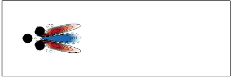
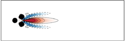
The steady solution becomes unstable beyond , as reported in § 2. A linear stability analysis indicates that one pair of complex-conjugated eigenmodes have a positive growth rate on the range , as shown in figure 7 for . These two leading eigenmodes are associated with vortical structures shed downstream in the wake, at the angular frequency 1/2. As the instability grows, the distorted mean flow changes, as expected by Eq. (3) and (19). The shift mode , involved in at , is shown in figure 8(c). In the permanent (time-periodic) flow regime, the distorted mean flow eventually matches the asymptotic mean flow field , and vortex shedding is well established with frequency .
| (a) |
 |
| (b) | |
| A | 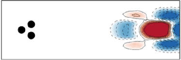 |
| B | 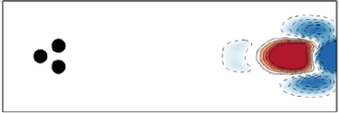 |
| C | 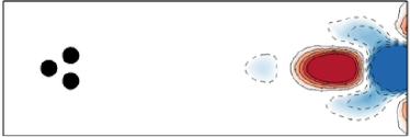 |
| (a) |
 |
| (b) |
 |
| (c) |
 |
4.2 Reduced-order model (ROM) of the primary flow regime
As introduced in § 3, the Galerkin ansatz for the Hopf bifurcation reads:
| (33) |
The von Kármán modes could be chosen as the real and imaginary part of the first eigenmode, respectively. This choice would make sense to describe the transient dynamics close to the steady solution. A better choice for describing the dynamics on the asymptotic limit cycle is to choose as the first two modes of a Proper Orthogonal Decomposition (POD) of the limit cycle data. The first two POD modes actually contribute to almost 95% of the total fluctuating kinetic energy at and are clearly associated with the von Kármán street of shed vortices, as shown in figure 8 (a)&(b). For the construction of the ROM, POD modes are preferred to the two leading eigenmodes, because we demand an accurate representation of the asymptotic periodic dynamics. Following Eq. (23)-(24), the dynamical system resulting from the Galerkin projection of ansatz (33) on the Navier-Stokes equations, after Krylov-Bogoliubov simplifications, reads
| (34) | |||||
| (35) | |||||
| (36) |
with and . The value of the coefficients at for the resulting ROM are summarized in table 2. Note that all coefficients but and are fixed by either the linear stability analysis or the asymptotic dynamics, see § 3. The coefficient can be chosen arbitrarily large as is slaved to (here we chose ), while had to be calibrated in order to better match the asymptotic angular frequency.
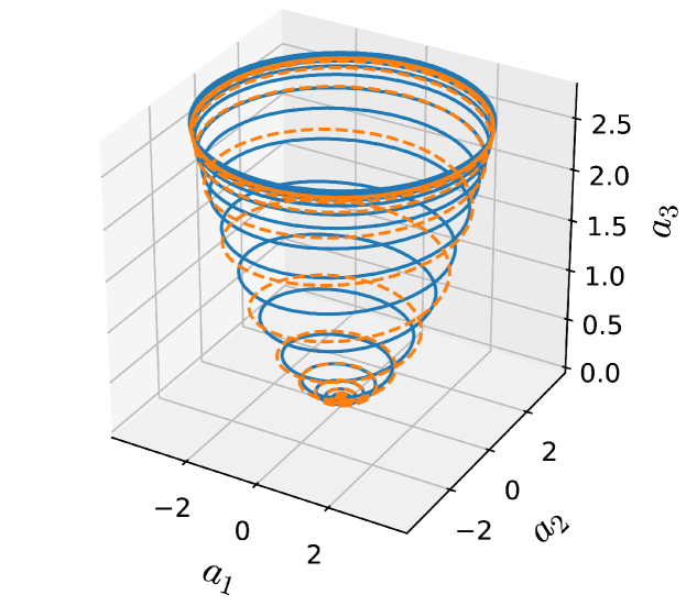
The dynamics of both the fluidic pinball (solid blue curve) and the ROM (dashed red curve) are compared in the three-dimensional subspace spanned by , , , see the top of figure 9. In figure 9 are also shown the individual time series of to for both the fluidic pinball and the ROM (same representation). As expected from the POD modes , the dynamics on the asymptotic (permanent) limit cycle is well described in amplitude and angular frequency by the ROM. Moreover, the ROM also captures the transient dynamics on the parabolic manifold . Henceforth, although all coefficients but one are fixed, the Galerkin system (33) is able to reproduce the most salient dynamical features of the flow in both the transient and the permanent regimes.
 |
 |
5 Secondary flow regime
The secondary flow regime ranges over . For illustration, we focus on the flow at , i.e. at a finite distance from the secondary bifurcation. In § 5.1 a linear stability analysis of the resulting three steady solutions is performed. A least-order model is proposed and discussed in § 5.2.
5.1 Eigenspectra of the steady solutions
As a result of the pitchfork bifurcation, there exist three steady solutions beyond : the symmetric steady solution , unstable to the periodic vortex shedding beyond , and two mirror-conjugated asymmetric steady solutions , also unstable to vortex shedding but only existing beyond , see figure 3.
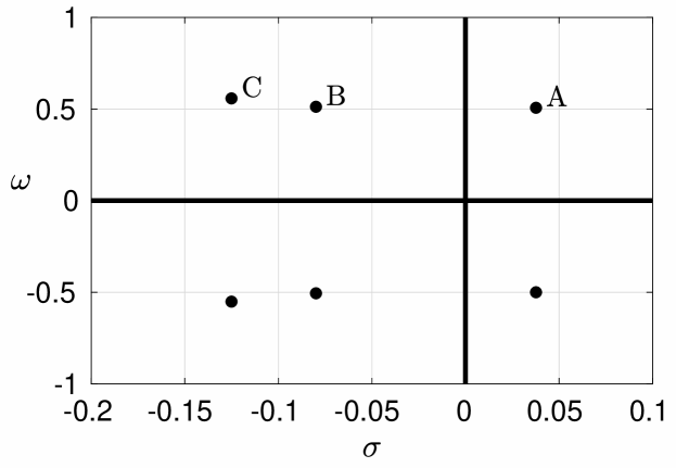
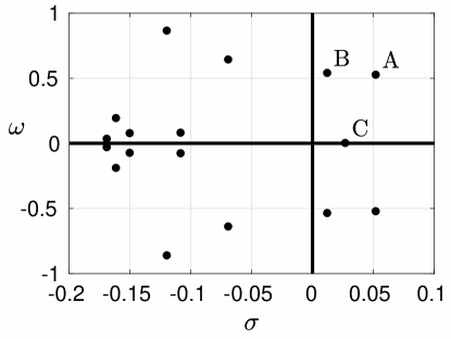
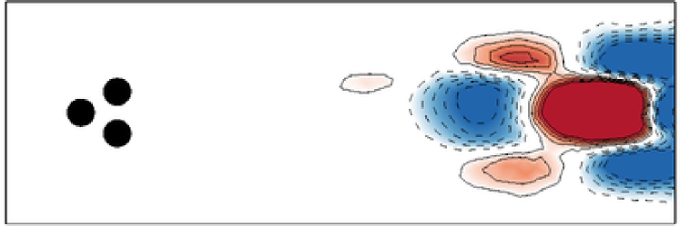
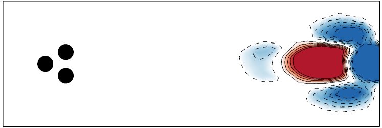
The linear stability analysis on reveals two pairs of complex-conjugated eigenmodes with positive growth rate, and one eigenmode of zero frequency, see figure 10(a). The steady eigenmode is antisymmetric and reflects the symmetry broken by the pitchfork bifurcation. It is clearly associated with the base-bleeding jet, with all its energy concentrated in the near-field. The two pairs of complex-conjugated eigenmodes are each associated with von Kármán streets of shed vortices. Both pairs of complex eigenmodes are antisymmetric and have quite similar angular frequencies. A closer view of the second pair of complex eigenmodes indicates that its growth rate cancels when the real eigenmode crosses the zero axis. This indicates that the new oscillatory mode is intimately connected to the symmetry breaking occurring at . At , this gives rise to the only stable limit cycle for the flow dynamics, while the limit cycle associated with the leading pair of complex eigenmode has become unstable and can only be visited transiently in time.
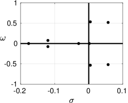
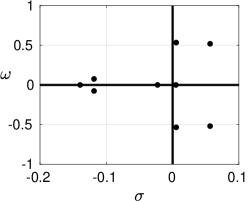
The linear stability analysis on (resp. ) reveals two pairs of complex-conjugated eigenmodes with positive growth rate, centered on an asymmetric mean flow, see figure 10(b). All eigenmodes are asymmetric, a property inherited from the steady solution.
In the permanent regime, the mean flow field will inherit the symmetry of one of the three (unstable) steady solutions, depending on the details of the initial perturbation.
| (a) | (b) | ||||||
 |
 |
||||||
|
A-
 B-
B-
|
5.2 Reduced-order model in the secondary flow regime
| (a) |
 |
| (b) |
 |
As discussed in § 3, an ansatz of the flow state can now be written as:
| (37) |
It is worthwhile noticing that, in the frame of this ansatz, the two asymmetric steady solutions are related to the symmetric steady solution via the additional antisymmetric mode :
| (38) |
where and are the time-averaged coefficients in the permanent regime. Consequently, can be easily computed as:
| (39) |
and further orthonormalized to , , by a Gram-Schmidt procedure. The resulting mode is shown in figure 11(a). A comparison with the eigenmode associated with the real eigenvalue, in figure 10(a), shows that the shift mode is just the real eigenmode against which the symmetric steady solution is unstable at , as expected by the definition of mode .
In a similar way, the additional mode can be constructed as:
| (40) |
Mode is shown in figure 11(b) after orthonormalization.
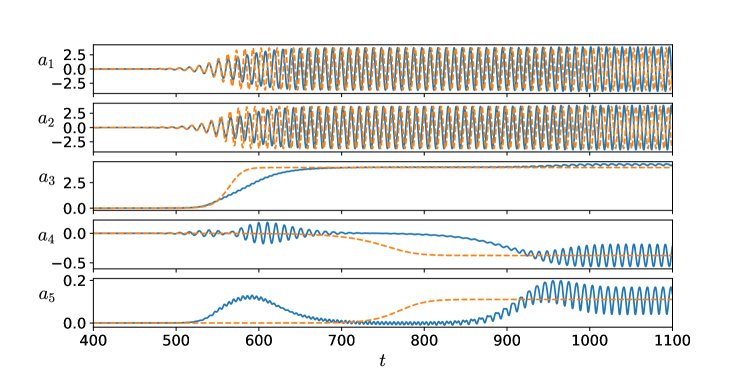
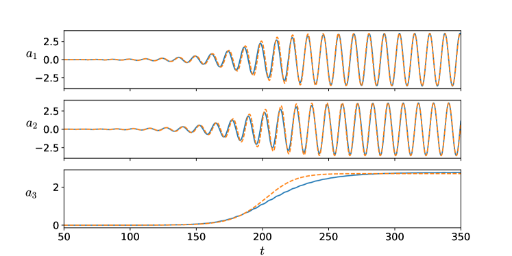
Close to the pitchfork bifurcation, the resulting dynamical system is described by Eqs. (32). At the threshold, the degrees of freedom , associated with the pitchfork bifurcation are expected to be fully uncoupled to the degrees of freedom , , associated with the Hopf bifurcation, and reciprocally, see § 3.3. In this case, an accurate linear and nonlinear dynamics from a Galerkin projection relies on deformable modes from eigenmodes near the fixed point to POD modes near the limit cycle (Loiseau et al., 2018). We avoid this complication by model identification from simulation data. The coefficients of the mean-field system (32) reported in table 3 were identified from the linear stability analysis of the symmetric steady solution and the asymptotic dynamics on the unstable symmetric preserving limit cycle and the stable symmetric-breaking limit cycle (see § 3.3 to 3.5). The resulting ROM dynamics is compared to the flow dynamics in figure 12. Inspection of figure 12 shows that such a model, reduced to only five degrees of freedom, is able to reproduce many features of the original dynamics: both the early transient and asymptotic dynamics of to are well reproduced, as well as the large timescale evolution of . However, the growth of coefficients to appears to be faster for the ROM, and , also reach their asymptotic value significantly sooner than their values for the full simulations of the fluidic pinball. In addition, the transient kick in is absent from the mean-field system (32), as well as the transient and asymptotic oscillations of and visible in figure 12, which would require coupling to or , or both. All these features indicate that at Reynolds number , the Krylov-Bogoliubov assumption of pure harmonic behaviour with slowly varying amplitude and frequency no longer holds.
As a consequence, cross-terms must be included in the ROM. The assumption of non-oscillatory dynamics of the shift mode amplitude and of the two pitchfork modes , is relaxed to reproduce the oscillatory behaviour evidenced in figure 12. Following § 3.6, the model identification process reads:
-
Step 1:
Keep the five-dimensional linear-quadratic form of the dynamical system from the Galerkin projection with 25 linear and 75 quadratic terms.
-
Step 2:
Remove vanishing terms arising from the symmetry of the modes. Thus, only 13 linear and 36 quadratic terms are left to be determined.
-
Step 3:
Enforce the linear dynamics of the unstable Hopf and pitchfork eigenmodes from stability analysis in the Galerkin system. This implies that the growth rate and frequency characterize the initial growth and angular frequency of , and represents the linear growth rate for .
-
Step 4:
The slaving of the Reynolds-stress-induced modes and to the fluctuation level is imposed by setting the damping rate 10 times larger than the growth rate of the corresponding fluctuation: , . This strong damping rate quickly forces the trajectory onto the mean-field manifold.
-
Step 5:
Enforce phase invariance for , in the first two equations. This is implied by the mean-field theory and is found to be a good approximation from numerical inspection. Thus, the oscillatory dynamics of , are governed by , , , , , , and .
-
Step 6:
Impose the asymptotic dynamics of the unstable symmetric limit cycle by fixing , , and .
-
Step 7:
Apply the SINDy algorithm (Brunton et al., 2016) to the remaining unknown terms, i.e. 6 linear terms and 28 quadratic terms. This step alone typically fails to yield a physics-based globally stable Galerkin system. This is not surprising in view of the necessary and sufficient conditions for global boundedness of Galerkin systems by Schlegel & Noack (2015). A Galerkin system identification with -norm penalization of the coefficients is found to have a performance similar to SINDy for the chosen constraints.
-
Step 8:
Two additional simplifying physics-based constraints are found to make the dynamic system identified by SINDy robust for a large range of initial conditions. Enforcing avoids the initial oscillatory dynamics being influenced by the initial kick of , and setting leads to the right asymptotic transition of the pitchfork bifurcation.
The resulting ROM reads:
| (41a) | |||||
| (41b) | |||||
| (41c) | |||||
| (41d) | |||||
| (41e) | |||||
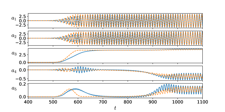
where . The coefficients are summarized in table 4. The dynamics of the system (41) (dashed red line) is compared to the full flow dynamics of the fluidic pinball (solid blue line) in figure 13. Now the initial stage of the dynamics is much better reproduced, as well as the asymptotic oscillations of , and . Interestingly, the faster growth in to , on the time-range around 600, could not be completely corrected. It is worthwhile noticing that this range of time also corresponds to oscillations in , which could not be reproduced by any cross-terms compatible with the symmetries of the system. Noticing that on this range of time may also question our choice for , which is the linear growth rate of the leading eigenmode around the symmetric steady solution . Indeed, although the initial condition is close to this point, the large amplitude oscillations of on the time range around 600 mean that the trajectory transiently escapes the symmetric subspace not only along , but also along and , before coming back close to the axis, on the time range from 700 to about 800. Therefore, it would be reasonable here to keep all the coefficients of the model unconstrained, but the number of free parameters is now too large for the identification process to be computationally tractable — for instance, it provides positive when it must necessarily be strongly negative.
Model identification can be very challenging for a number of reasons. First, the conditions for global boundedness of the attractor for the linear-quadratic Galerkin system are rather restrictive (Schlegel & Noack, 2015). Second, the Galerkin method assumes fixed expansion modes. Yet, least-order models often have deformable modes changing with the fluctuation level (Tadmor et al., 2011). The von Kármán vortex shedding metamorphosis from stability modes to POD modes may serve as an example. These deformations may also affect the structure of the dynamical system. Third, the Navier-Stokes dynamics may live on a strongly attracting manifold. This restriction of the state space may make certain Galerkin system coefficients numerically unobservable, like and in our case. Despite these challenges, the model identified in table 4, as exemplified by figure 13, constitutes a faithful least-order model for the fluidic pinball at . Although the model is only five-dimensional, it can reproduce most of the key features, timescales, transient and asymptotic behaviour of the full dynamics.
6 Conclusions and outlooks
Reduced-order models (ROM) serve a number of purposes. For instance, ROMs facilitate a deeper understanding of the physical mechanisms at play in a flow configuration, by extracting the low-dimensional manifold on which evolve the dynamics (Manneville, 2010). In that respect, the linear stability analysis of the steady solution shows the nonlinear amplitude saturation mechanism through the distorted mean flow. The difference between steady solution and the mean flow is caused by the Reynolds stress, captured by the shift mode , and affects the stability properties (Noack et al., 2003; Barkley, 2006; Sipp & Lebedev, 2007; Turton et al., 2015). Deeper investigations would certainly deserve to be carried out on the relation between the stability analysis of fixed points, Floquet analysis of limit cycles and Lyapunov exponents of chaotic flow regimes. In addition, because Hopf and pitchfork bifurcations are generic bifurcations in fluid flows, the nonlinear dynamics identified in this study are expected to be extended and generalizable to other flows exhibiting similar bifurcations. Last but not least, a ROM provides fast estimators for predicting the forward evolution of the system. Such estimators could be used for control purposes (Brunton & Noack, 2015; Rowley & Dawson, 2017). All these considerations motivated the present study, whose main results are summarized in § 6.1. Outlooks of this work are listed in § 6.2.
6.1 Concluding remarks and discussion
Flow configurations undergoing successive Hopf and pitchfork bifurcations are common in fluid mechanics. This is, for instance, the case of three-dimensional wake flows such as spheres (Mittal, 1999; Gumowski et al., 2008; Szaltys et al., 2012; Grandemange et al., 2014) or bluff body wake flows (Grandemange et al., 2012, 2013; Cadot et al., 2015; Bonnavion & Cadot, 2018; Rigas et al., 2014). The drag crisis and stalled flows are also characterized by the pitchfork bifurcation of a primarily Hopf-bifurcated flow, but the secondary transition is subcritical in this case.
In this study, we have considered the fluidic pinball on its way to chaos and have identified least-order models of the flow dynamics in the primary Hopf-bifurcated and secondary pitchfork-bifurcated flow regimes. Reduced-order modeling of Hopf bifurcations was already addressed in Noack et al. (2003) for the cylinder wake flow, while Meliga et al. (2009) derived the amplitude equation for a codimension two bifurcation (pitchfork and Hopf) based on a weakly nonlinear analysis in the wake of a disk, and Fabre et al. (2008) derived the same equation solely based on symmetry arguments, in the wake of axisymmetric bodies. In the present contribution, we could demonstrate that the dynamics resulting from the successive Hopf and pitchfork bifurcation could be well-captured by a five-dimensional model whose degrees of freedom couple through quadratic non-linearities, as imposed by the Navier-Stokes equations.
For the fluidic pinball, the route to chaos is characterized by a primary supercritical Hopf bifurcation at , followed by a secondary supercritical pitchfork bifurcation at . The Hopf bifurcation corresponds to the destabilization of the steady solution with respect to vortex shedding, while the pitchfork bifurcation occurs when the mean flow breaks the symmetry with respect to the mirror-plane. The fluctuation amplitude of the von Kármán street is reduced, over a finite range of the Reynolds number around , when the base-bleeding jet is rising. This means that energy is withdrawn from the fluctuations to feed the mean flow transformation. Before the next transition occurs, the fluctuation amplitude starts to grow again, up to the largest value of the Reynolds number considered in this work.
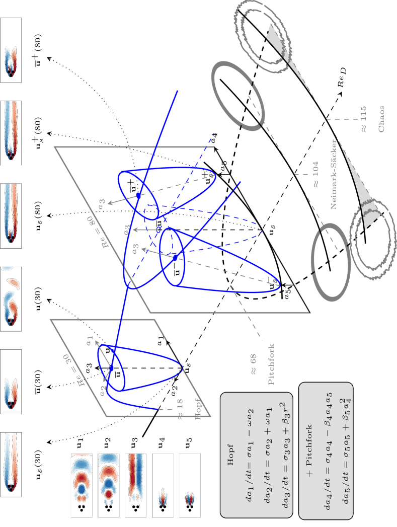
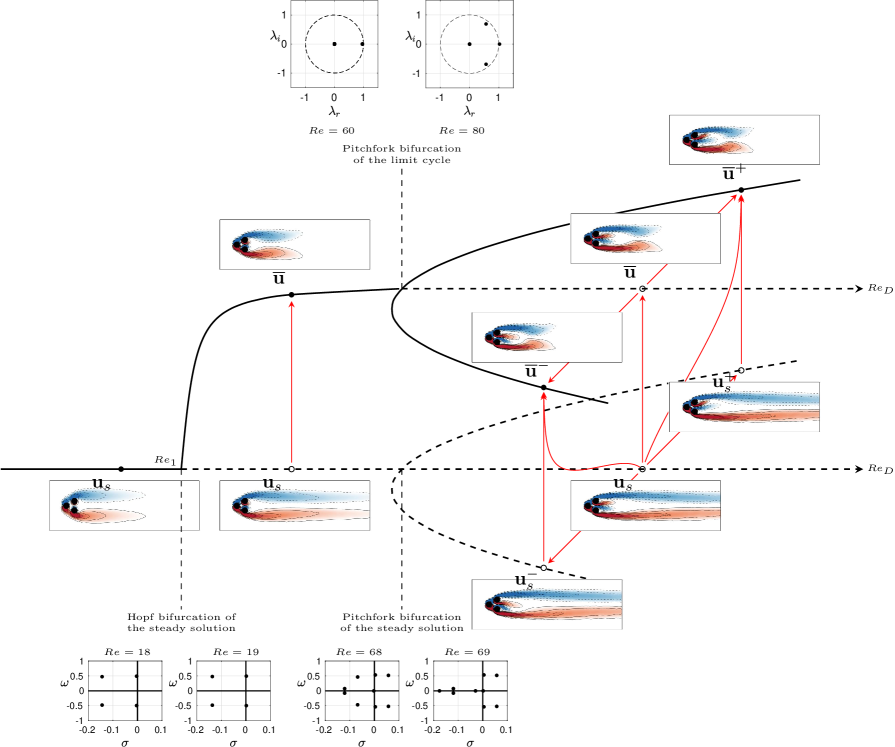
There is strong evidence that the next transition is a Neimark-Säcker bifurcation. The resulting flow regime is most likely quasi-periodic over the range . In this regime, a new oscillatory phenomenon takes place, characterized by slow oscillations of the base-bleeding jet. Three additional degrees of freedom might be necessary to deal with the newly arising oscillator. The flow dynamics eventually bifurcates into a chaotic regime, characterized by the random switching of the base-bleeding jet between two symmetric deflected positions. The overall route to chaos is summarized in the phenomenogram of figure 14.
The reduced-order models derived by Galerkin projections of the Navier-Stokes equations, based on the symmetry of the individual degrees of freedom, under Krylov-Bogoliubov simplifications, faithfully extract the manifolds on which the flow dynamics sets in. The ROM for the primary flow regime is only three dimensional: two degrees of freedom are associated with the asymptotic stable limit cycle resulting from the vortex shedding. The third degree of freedom is a mode slaved to the two dominant modes and is mandatory for the description of the transient flow dynamics from the unstable steady solution to the post-transient mean flow, as already demonstrated in Noack et al. (2003). The least-order model in the secondary flow regime has only five degrees of freedom, three of which are associated with the Hopf bifurcation, the two remaining degrees of freedom being associated with the pitchfork bifurcation. In the phenomenogram of figure 14 are reported the structure of both reduced-order models close to the Hopf and the pitchfork bifurcations. When the two sets of degrees of freedom are fully uncoupled, some features of the flow dynamics are well-reproduced (asymptotic mean behaviour, parabolic manifolds of the Hopf and pitchfork bifurcations), but many details are missing. To reproduce most of the transient and asymptotic flow features far from the bifurcation point, additional cross-terms have been included in the model, which relaxes the steadiness constraint usually assumed for the shift modes.
6.2 Outlook
The current generalized mean-field model captures the Hopf bifurcation and subsequent pitchfork bifurcation of the steady solution and limit cycles. The following onset of a quasi-periodic regime with slow oscillations of the deflected base-bleeding jet might presumably be incorporated by another Hopf bifurcation, leading to a 8-dimensional mean-field Galerkin model. The transition to chaos is accompanied by a return to a statistically symmetric flow, i.e. the base-bleeding jet oscillates around one asymmetric state before it stochastically switches to the other mirror-symmetric one. This behaviour is reminiscent of the transition to chaos of a harmonically forced Duffing oscillator. In the case of the fluidic pinball, the vortex shedding would constitute a forcing. Hence, one may speculate that the transition to chaos may already be resolved by the 8-dimensional Galerkin model in which the effect of vortex shedding on the jet oscillation becomes stronger with an increasing Reynolds number.
An alternative direction is to increase the accuracy of the mean-field Galerkin model. While the structure of the Galerkin system prevails for a large range of Reynolds numbers, the modes and all Galerkin system coefficients change in a non-trivial manner, e.g., the growth-rate formula should read . The transients can be expected to be much more accurately resolved by the mean flow dependent modes, e.g. , for the resolution of vortex shedding (Loiseau et al., 2018). More generally, the flow lives on a low-dimensional manifold which includes mode deformations (Noack, 2016). Locally linear embedding (LLE) is a powerful technique for identifying the dimension and a parameterization in an automatic manner (Roweis & Saul, 2000). The normal form of the bifurcations can be expected to coincide with the dynamics on the LLE feature coordinates.
A third direction follows an observation of Rempfer (1994) that Galerkin systems of many fluid flows can be considered as nonlinearly coupled oscillators. For two incommensurable shedding frequencies, this observation has been formalized in a generalized mean-field model by Noack et al. (2008); Luchtenburg et al. (2009). Such multi-frequency models may be extended to resolve broadband frequency dynamics taking, for instance, the most dominant DMD modes (Rowley et al., 2009; Schmid, 2010). Strengths and weaknesses of techniques currently used for model reduction are discussed in Taira et al. (2017). While mean-field consideration expressly ignores non-trivial triadic interactions, their quantitative effect on the frequency crosstalk may still be well approximated by the mean flow interaction terms. Such multi-frequency mean-field models may eventually describe the effect of open-loop forcing on turbulence, see for instance the recent thorough review by Jiménez (2018) on turbulent flow modeling.
A fourth direction aligned with the large success of machine learning / artificial intelligence is the automated learning of state spaces, modes, and dynamical systems. For the latter, SINDy provides an established elegant framework (Brunton et al., 2016). The choice of the state spaces might be facilitated by manifold learning from many solution snapshots (Gorban & Karlin, 2005). The authors actively pursue all the mentioned directions.
Acknowledgements
This work is supported by a public grant overseen by the French National Research Agency (ANR) as part of the “Investissement d’Avenir” program, through the “iCODE Institute project” funded by the IDEX Paris-Saclay, ANR-11-IDEX-0003-02, by the ANR grants ‘ACTIV_ROAD’ and ‘FlowCon’ (ANR-17-ASTR-0022), and by Polish Ministry of Science and Higher Education (MNiSW) under the Grant No.: 05/54/DSPB/6492.
We appreciate valuable stimulating discussions with Steven Brunton, Alessandro Bucci, Nathan Kutz, Onofrio Semeraro, Yohann Duguet, Laurette Tuckerman and the French-German-Canadian-American pinball team: François Lusseyran, Guy Cornejo-Maceda, Jean-Christophe Loiseau, Robert Martinuzzi, Cedric Raibaudo, Richard Semaan, and Arthur Ehlert.
Appendix A Asymmetric steady solutions
For a Reynolds number larger than the critical value of the pitchfork bifurcation , we can obtain two additional asymmetric steady solutions, one associated with the base-bleeding jet deflected upward, the other downward. These two asymmetric steady solutions are obtained by the steady Navier-Stokes solver initialized with a flow field (snapshot) with the same state of the base-bleeding jet. From the two asymmetric vortex shedding, their corresponding asymmetric steady solutions can be obtained by the following steps:
-
Step 1:
Run the unsteady Navier-Stokes solver with a time scale larger than the vortex shedding period, initialized from a snapshot of the asymmetric vortex shedding. The vortex shedding will quickly vanish for this artificially large time scale and approach the corresponding approximation of the steady state.
-
Step 2:
Run the steady Navier-Stokes solver, restarted from this vortex shedding vanished solution to further refine the steady state.
Initialized with the three steady solutions with different states of the base-bleeding jet at , the steady solutions for other Reynolds numbers can be obtained by the steady Navier-Stokes solver. At , all three steady solutions converge to a unique solution, which indicates that the critical value of the pitchfork bifurcation of the steady solution is between to , as shown in figure 15 based on the pressure lift coefficient of the steady solutions.
Appendix B Linear stability analysis
The linear stability problem for a base flow with small perturbations is governed by the linearized Navier-Stokes equations, which read:
| (42) |
The assumption of small perturbation allows to linearize the equations, and we can separate the time and space dependence as:
| (43) |
By introducing the linear operator , all the terms except the time derivative term and the continuity equation can be cast as , we can rewrite (42) as
| (44) |
Introducing (43) into (44), the equations can be written as:
| (45) |
We use subspace iteration to solve this eigenvalue problem. A detailed review can be found in Morzynski et al. (1999).
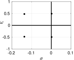
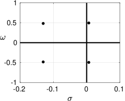
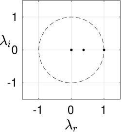
The global stability analysis of the steady solutions at different Reynolds numbers has been performed on a Krylov subspace of dimension 9-20. This converges after 50-100 iterations. The linear stability analysis on the symmetric steady solution reveals a pair of conjugated eigenvalues with positive real part first appearing as the Reynolds number is changing from 18 to 19, see figure 16(a). A real eigenvalue becomes positive between and , see figure 16(b). This confirms that a Hopf bifurcation occurs on the symmetric steady solution at , and a pitchfork bifurcation at .
| (a) | 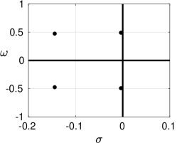 |
 |
 |
|---|---|---|---|
| (b) | 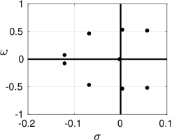 |
 |
 |
Appendix C Floquet stability analysis
Similar to the linear stability framework, the Floquet stability problem works with a T-periodic base flow . The linear operator now reads:
| (46) |
The linear operator is T-periodic because of the base flow . The solutions to (46) are seeked as:
| (47) |
with the T-periodic Floquet modes and the corresponding Floquet exponents . We define the Floquet operator as the time-integrated with the pre-stored periodic solutions over one period (Barkley & Henderson, 1996; Schatz et al., 1995), which reads:
| (48) |
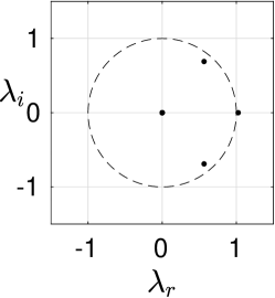
The method used to solve the eigenproblem is the same as the linear stability analysis. The Floquet multipliers of can be written as . In our case, we consider the multipliers .
We performed the iteration on a Krylov subspace of dimension 9, using a symmetry-constrained T-periodic base flow. Below the critical Reynolds number, the base-bleeding jet is approximately steady and symmetric. This symmetry is also enforced at higher Reynolds numbers to compute the unstable periodic solution. The constraint is imposed on the central line as:
| (49) |
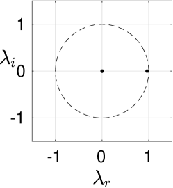
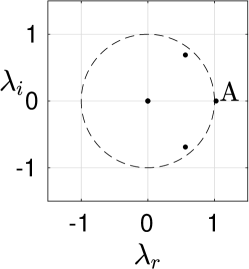
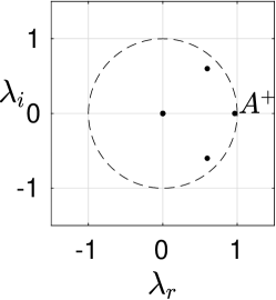
As (49) restricts the vertical velocity of the nodes, the symmetry-constrained periodic solution is very close to the symmetry-preserving periodic solution. Normally, 10-20 iterations are enough to get a converged leading eigenvalue, initialized with a random vector or a Ritz vector computed at nearby Reynolds number with the periodic solution of the same symmetry. We do not attempt to calculate a complete, converged spectrum of all the eigenvalues, as the leading eigenvalue is associated with the instability of interest. The multipliers from the Floquet analysis around the critical value of the pitchfork bifurcation are shown in figure 17. When increasing , the leading real eigenvalue crosses the unit cycle at as changes from 69 to 70. The critical value of the pitchfork bifurcation is, therefore, , identical to the critical value for the steady solution at the precision of the numerics. Both of them have the same eigenmode. At , the Floquet modes of both the unstable symmetric periodic solution and the stable asymmetric periodic solutions are shown in figure 18.
 |
 |
 |
| (a) | (b) | (c) |
| (a) | (b) | ||
 |
 |
||
|
A+
|
Overall, combined with the result of the linear stability analysis of the steady solutions, the bifurcation scenario at low Reynolds numbers can be shown in figure 19. The linear stability analysis on the steady solution and the periodic solution show a highly consistent result: the same kind of bifurcation with nearly the same critical Reynolds number, and the same eigenmodes. Besides, at , the growth rates of the real eigenmode are very close: 0.0272 from the symmetric steady solution, 0.0247 from the symmetric periodic solution. This similarity is understood as the result of a transverse effect of the symmetric subspace.
Appendix D Transient dynamics from different steady solutions
In this section, we show in figure 20 some typical transient dynamics starting with the unstable symmetric/asymmetric steady solutions at different Reynolds numbers, based on the pressure lift coefficient from the resulting force on the three cylinders. Combining with the pressure drag coefficient and the time-delayed lift coefficient in which is a quarter period, provides the phase portraits of figure 21. Three comparative numerical simulations are shown, starting with the symmetric and the two mirror-conjugated asymmetric steady solutions at the same respectively. The mirror-conjugated initial conditions provide mirror-conjugated transient dynamics.
| (a) | 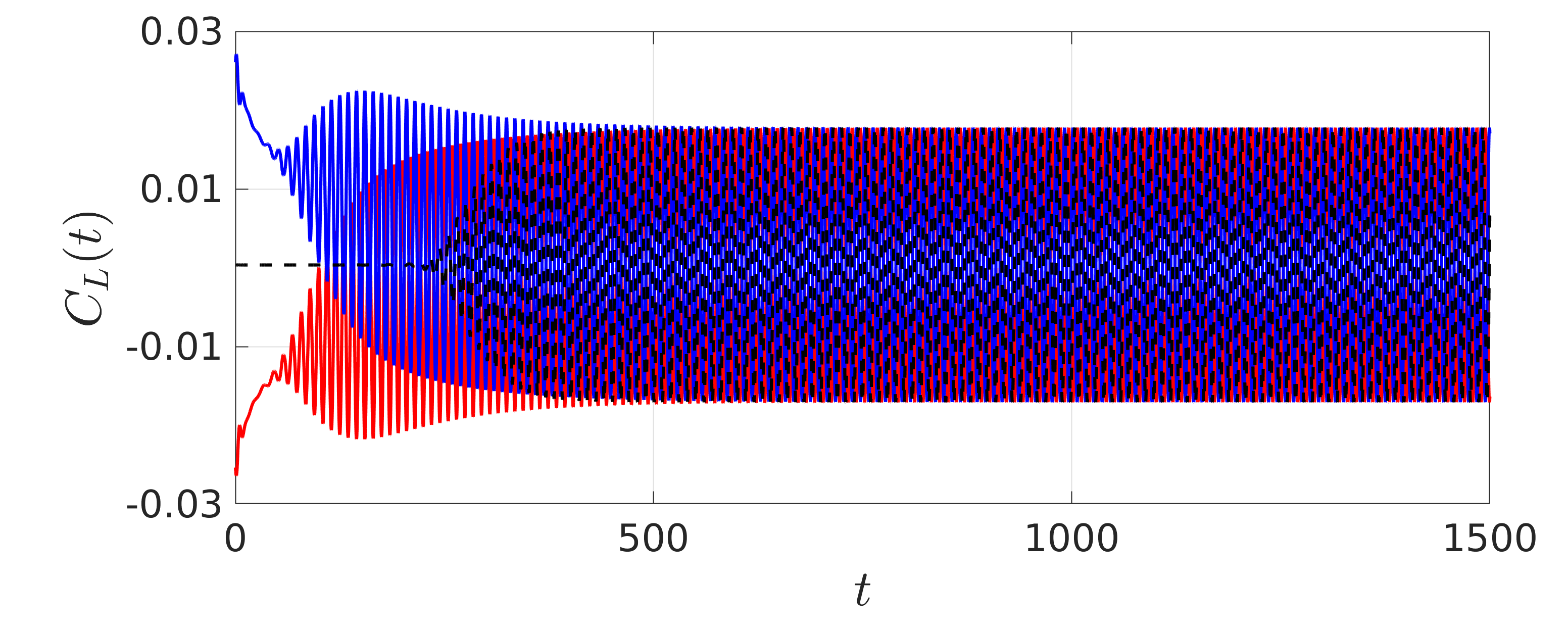 |
| (b) | 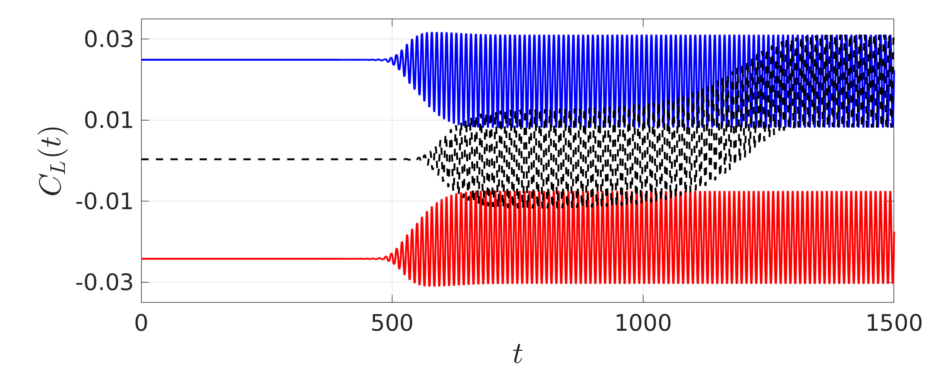 |
| (c) | 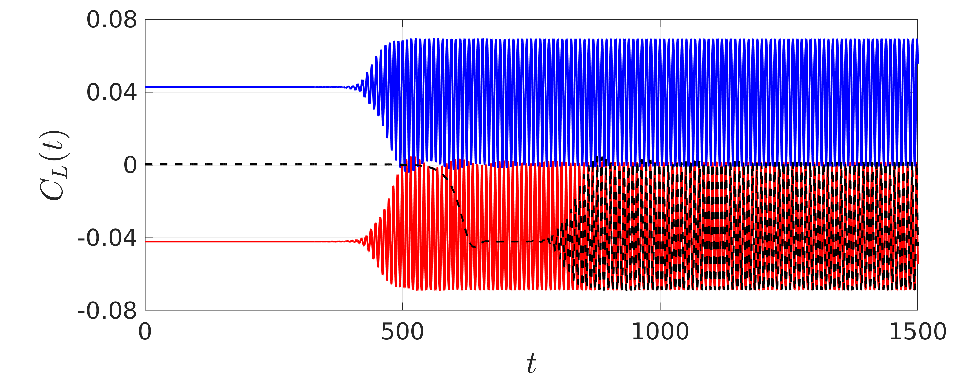 |
Figure 20(a) shows the transient dynamics at the critical Reynolds number , initialized with the three steady solutions at . The lift coefficient starts oscillating quickly, and eventually reaches a unique oscillating state with zero mean value. This is consistent with the Floquet analysis at , where only one stable symmetry-centered limit cycle exists and any other state will eventually converge to this stable state.
Figure 20(b) shows three different scenarios at depending on the initial condition: from the symmetric steady solution to the symmetry-centered limit cycle, from the symmetric centered limit cycle to the asymmetry-centered limit cycles, and from the asymmetric steady solutions to the asymmetry-centered limit cycles. Starting with the symmetric steady solution, it will first reach the unstable symmetry-centered limit cycle, before asymptotically approaching one of two stable asymmetry-centered limit cycles. However, starting with the asymmetric steady solutions, it will directly reach the corresponding stable asymmetry-centered limit cycle. If the initial perturbation introduced to the symmetric steady solution has a certain bias of symmetry, a transition from the symmetric steady solution to one of the two asymmetry-centered limit cycles will occur.
As we keep increasing the Reynolds number up to , there still exist six states, but the transient scenario from the symmetric steady solution is different. It will first reach one of two unstable asymmetric steady solutions , before asymptotically approaching the corresponding asymmetry-centered limit cycle, as shown in figure 20(c).
All these transient dynamics mentioned above are highlighted with the red arrows in figure 19.
| (a) | 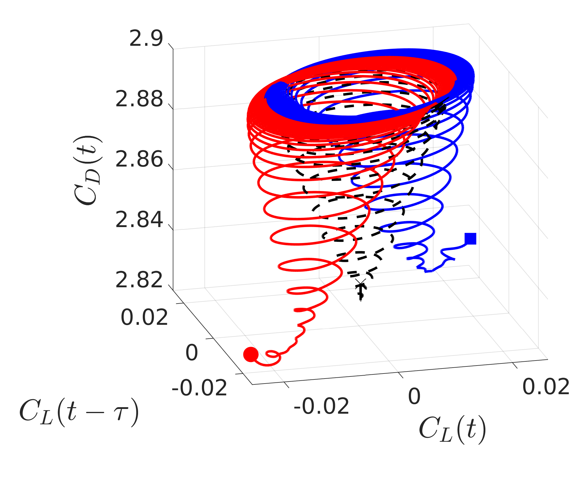 |
(b) | 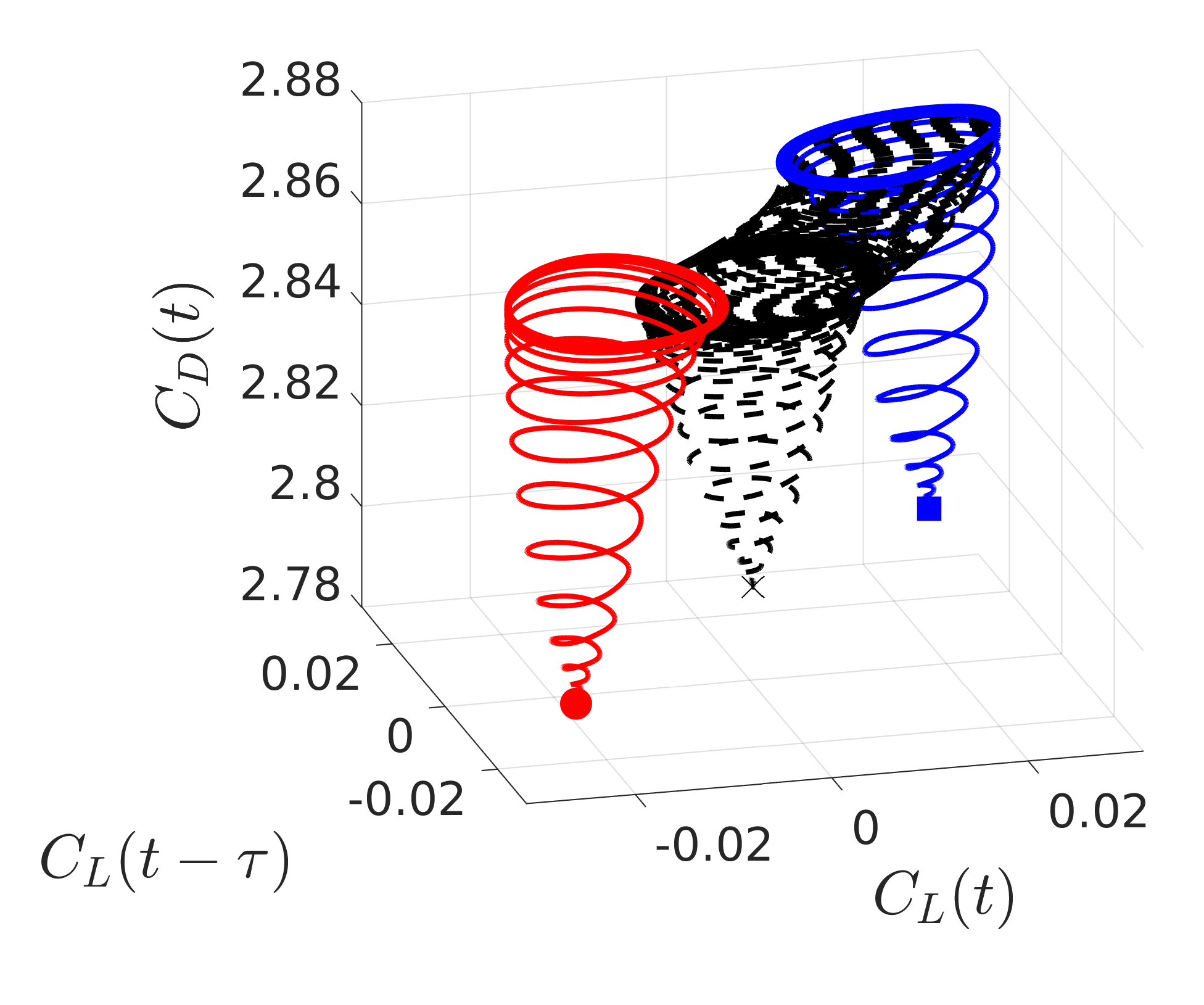 |
| (c) | 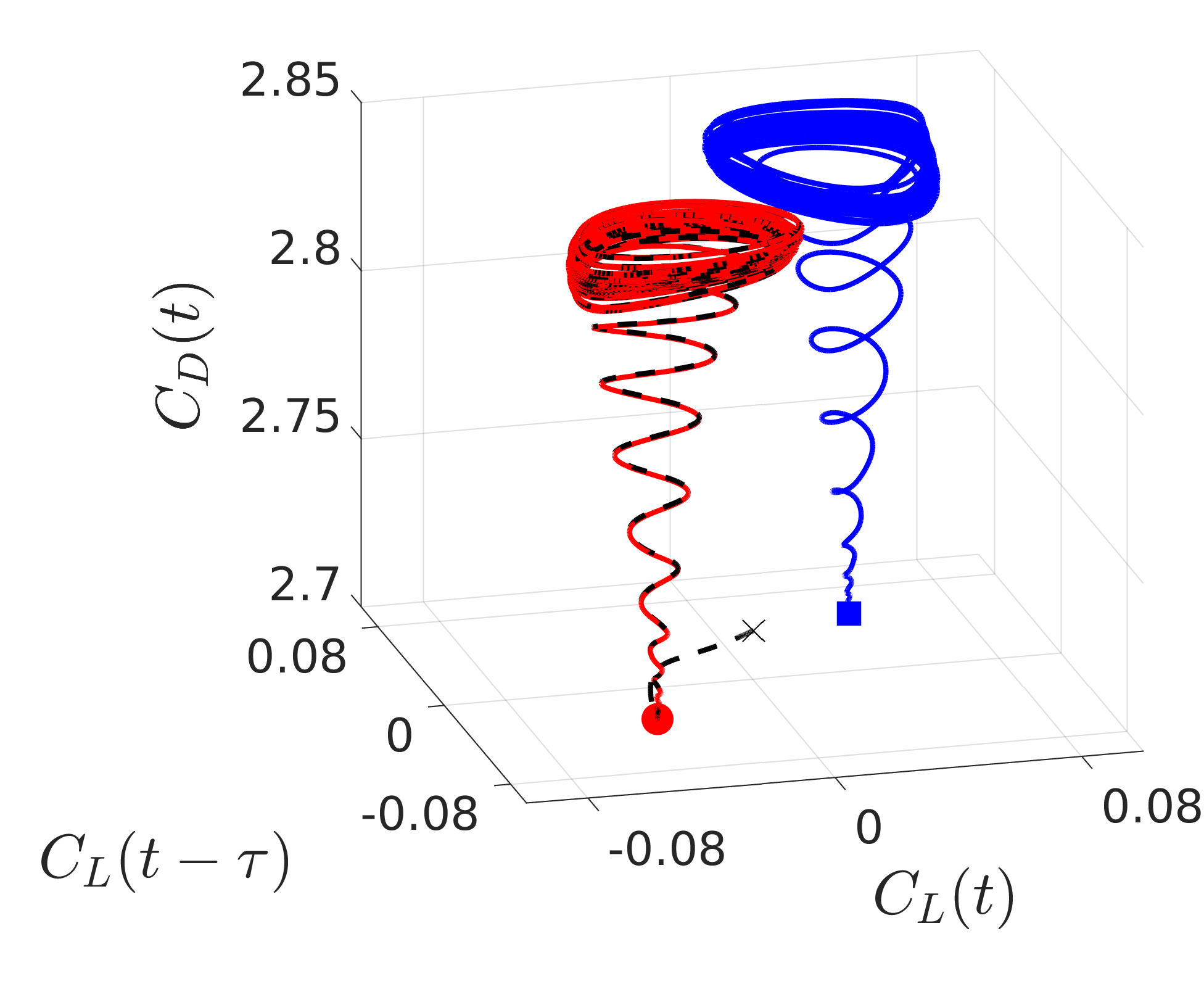 |
The phase portraits starting with different steady solutions, as shown in figure 21, reveal the above-mentioned transient dynamics which is affected by the initial condition and the Reynolds number. At the same time, it also reflects the global effect of the pitchfork bifurcation at , splitting the state space (see figure 21(a)) into a symmetric sub-space and two mirror-conjugated asymmetric sub-spaces (see figure 21(b),(c)).
Appendix E On the simultaneous instability of the fixed point and the limit cycle
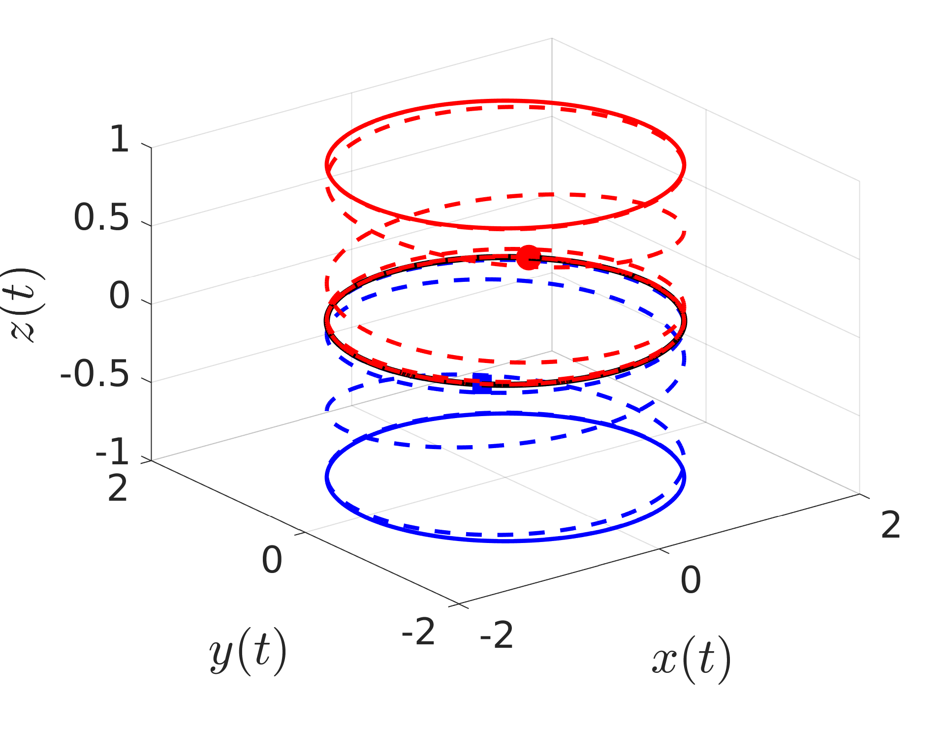
In this section, we exemplify the transverse effect of the pitchfork bifurcation on a three-dimensional dynamical system equivalent to the system of Eq. (32).
Dynamical system
The dynamical system reads:
| (50) |
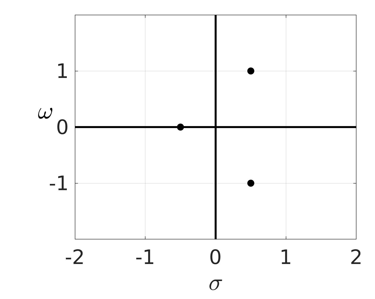
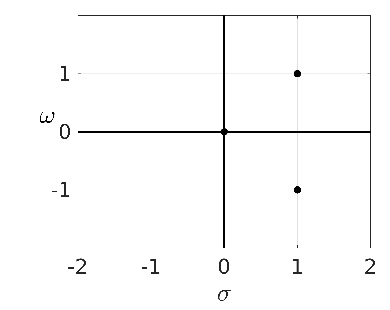
with . This system undergoes a supercritical Hopf bifurcation in the -plane at and a supercritical pitchfork bifurcation along the -axis at . For , the stable fixed point at becomes unstable, and the limit cycle around with radius and angular frequency is stable in the (x,y)-plane. Increasing until , the fixed point undergoes a secondary instability, as well as the limit cycle. Three unstable fixed points , , and three limit cycles around these fixed points with radius and angular frequency in the (x,y)-plane are found, as shown in figure 22.
Linear stability analysis
The ODE (50) can be writen as:
| (51) |
and we note is the steady state,that is, . Consider a small perturbation around the steady state by
| (52) |
We derived the linearized evolution equation:
| (53) |
where is the Jacobian matrix of the considered steady state .
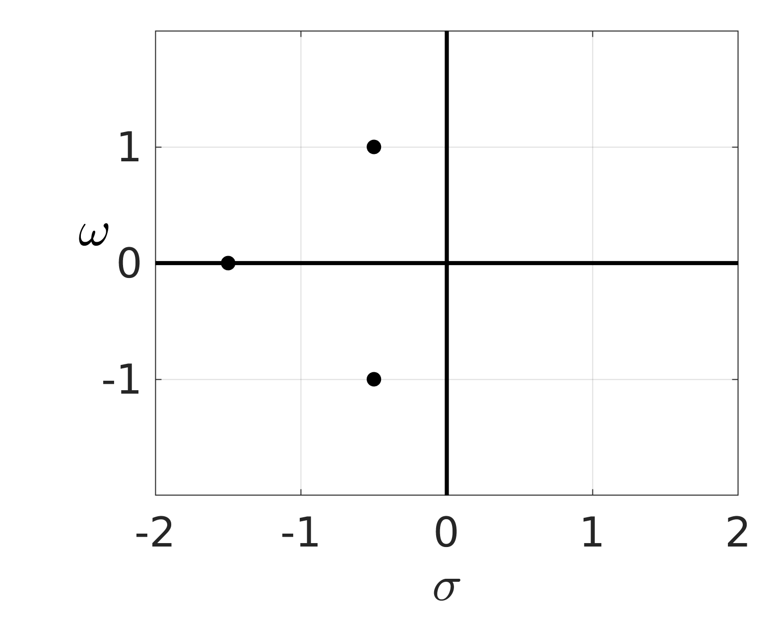
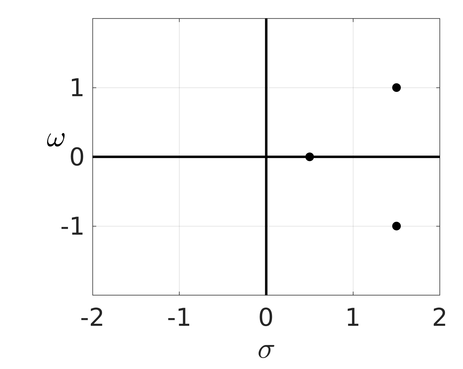
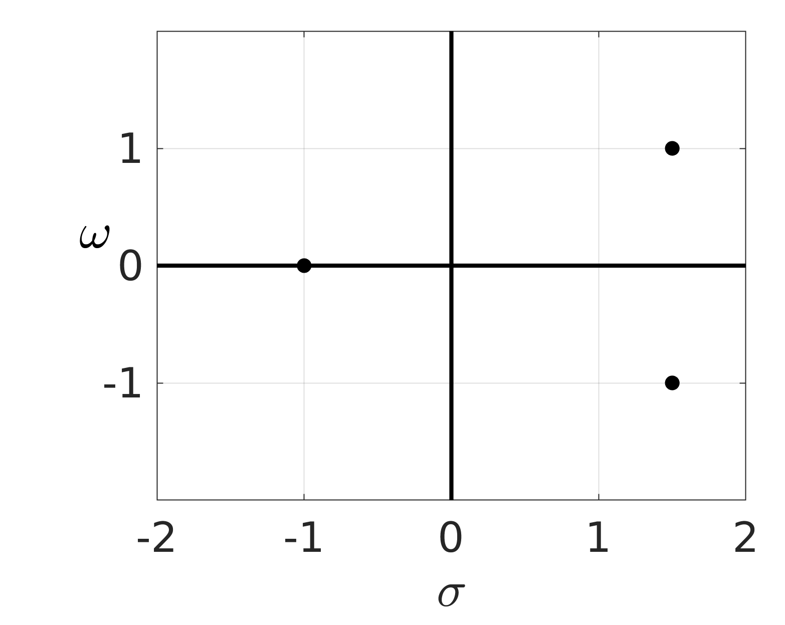
The stability of this steady state is determined by the eigenvalues of the Jacobian matrix. The eigenspectrum of the fixed point is shown in figure 23. The growth rate and angular frequency of the pair of conjugated eigenvalues are and respectively. The growth rate of the real eigenvalue is .
 |
 |
 |
| (a) | (b) | (c) |
 |
 |
| (d) | (e) |
The eigenspectrum of the steady solution for is shown in figure 26(right). The growth rate is at the steady solution and at the steady solution .
|
 |
Floquet stability analysis
Now, we consider the periodic solution of the system of (50), which can be writen as:
| (54) |
Consider a small perturbation around the periodic solution by
| (55) |
The first variational form reads:
| (56) |
where is the Jacobian matrix of the considered periodic solution , but now, the linear equation has periodic coefficients.
The monodromy matrix can be written as:
| (57) |
or equivalently:
| (58) |
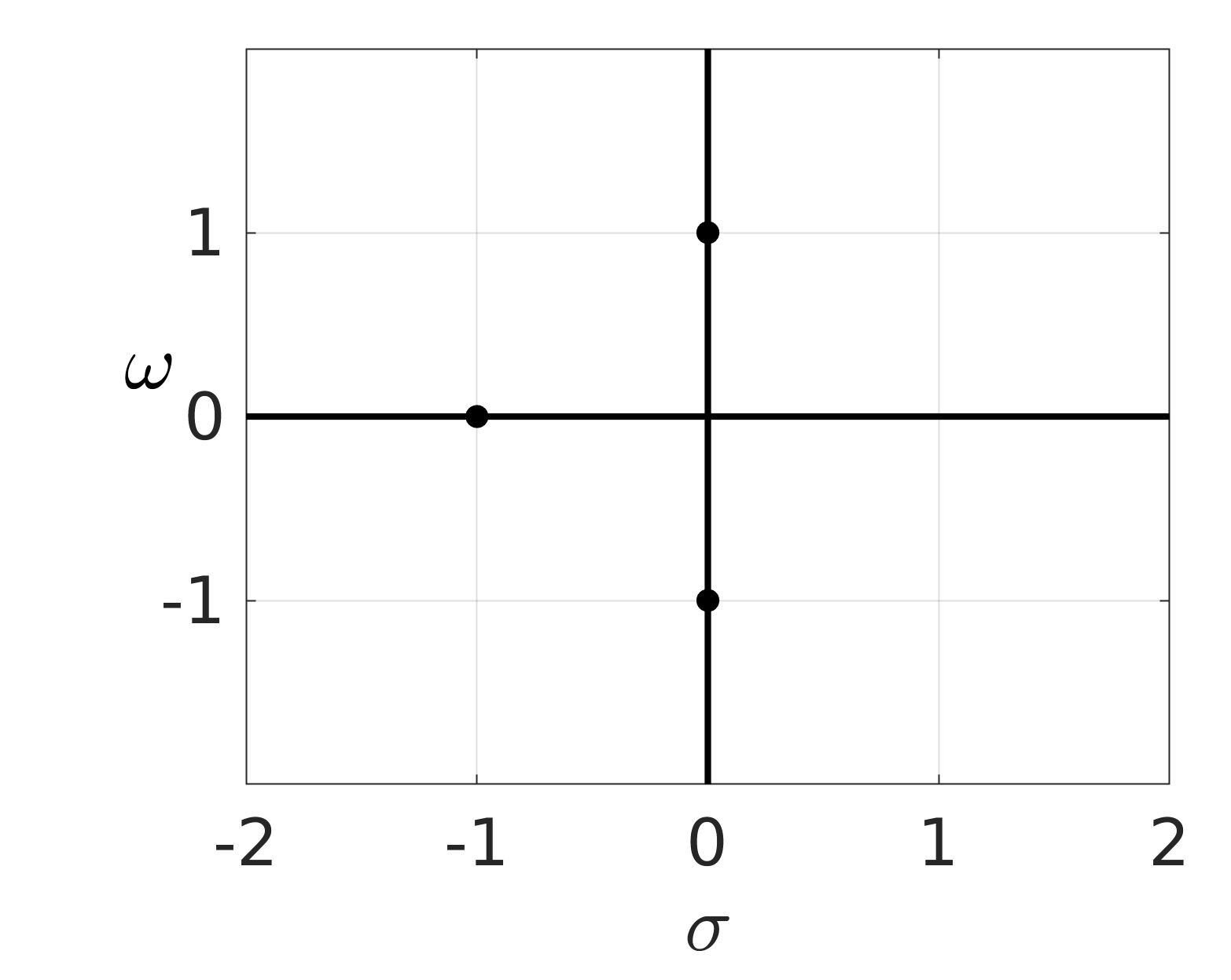
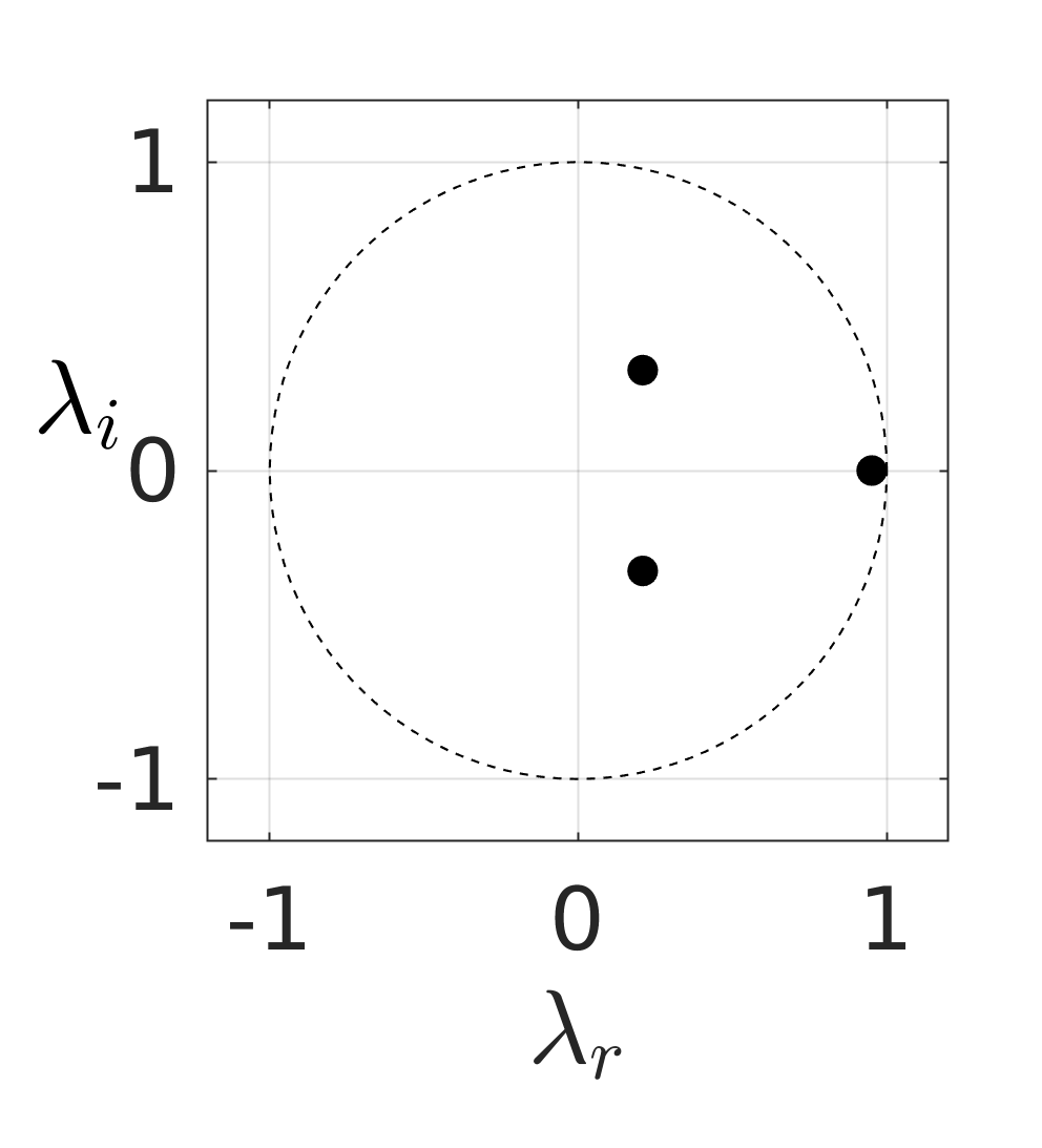
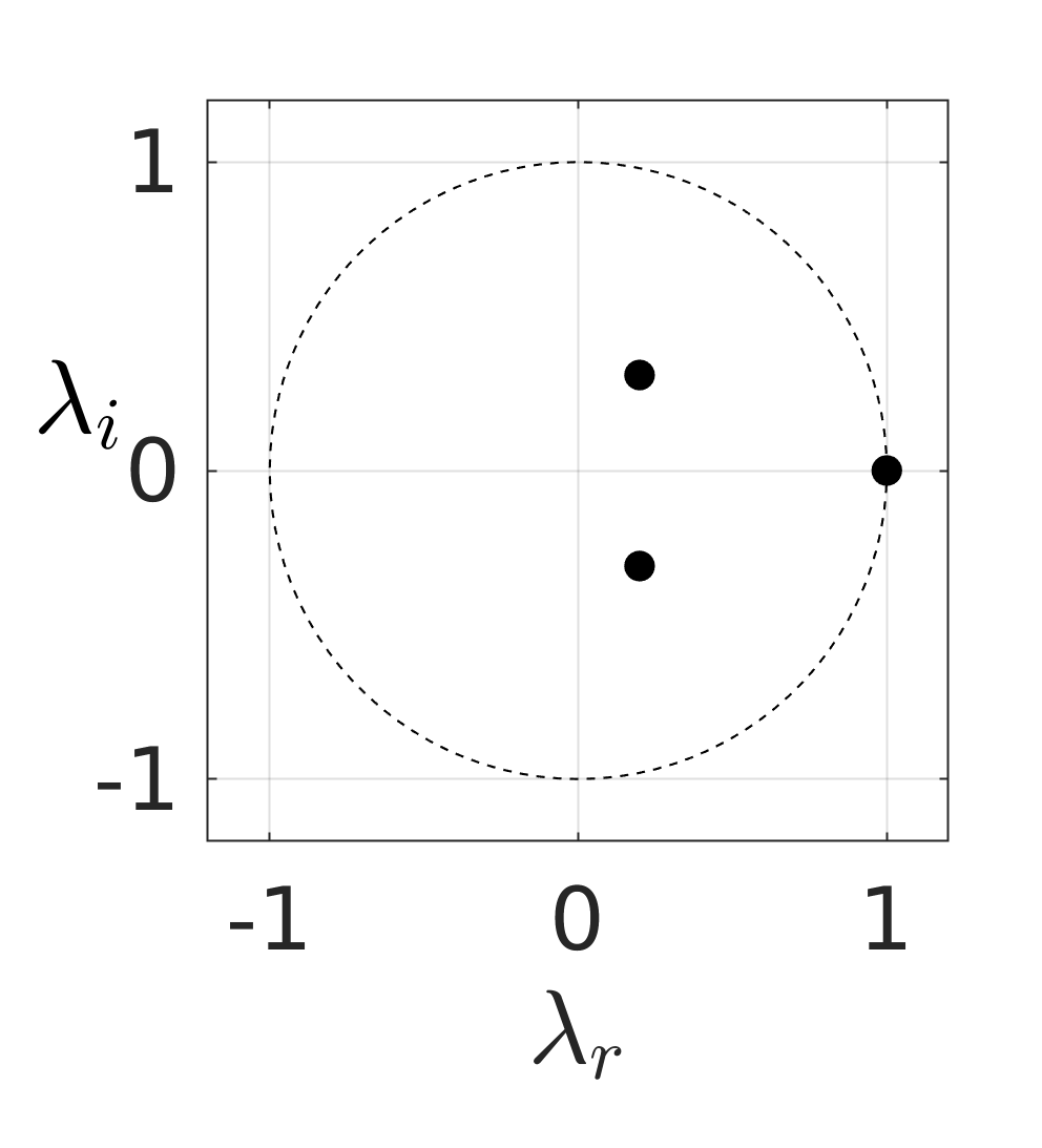
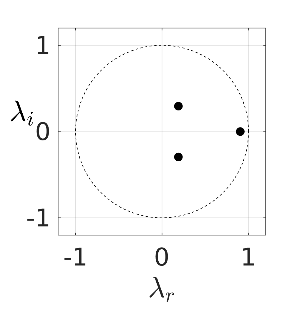
The stability of this periodic solution is determined by the multipliers , being the eigenvalues of the monodromy matrix. As shown in figure 25, the periodic solution : for becomes unstable. A real multiplier crosses the unit cycle at . The Floquet exponent of this real multiplier is , equal to the growth rate at the fixed point .
 |
 |
 |
| (a) | (b) | (c) |
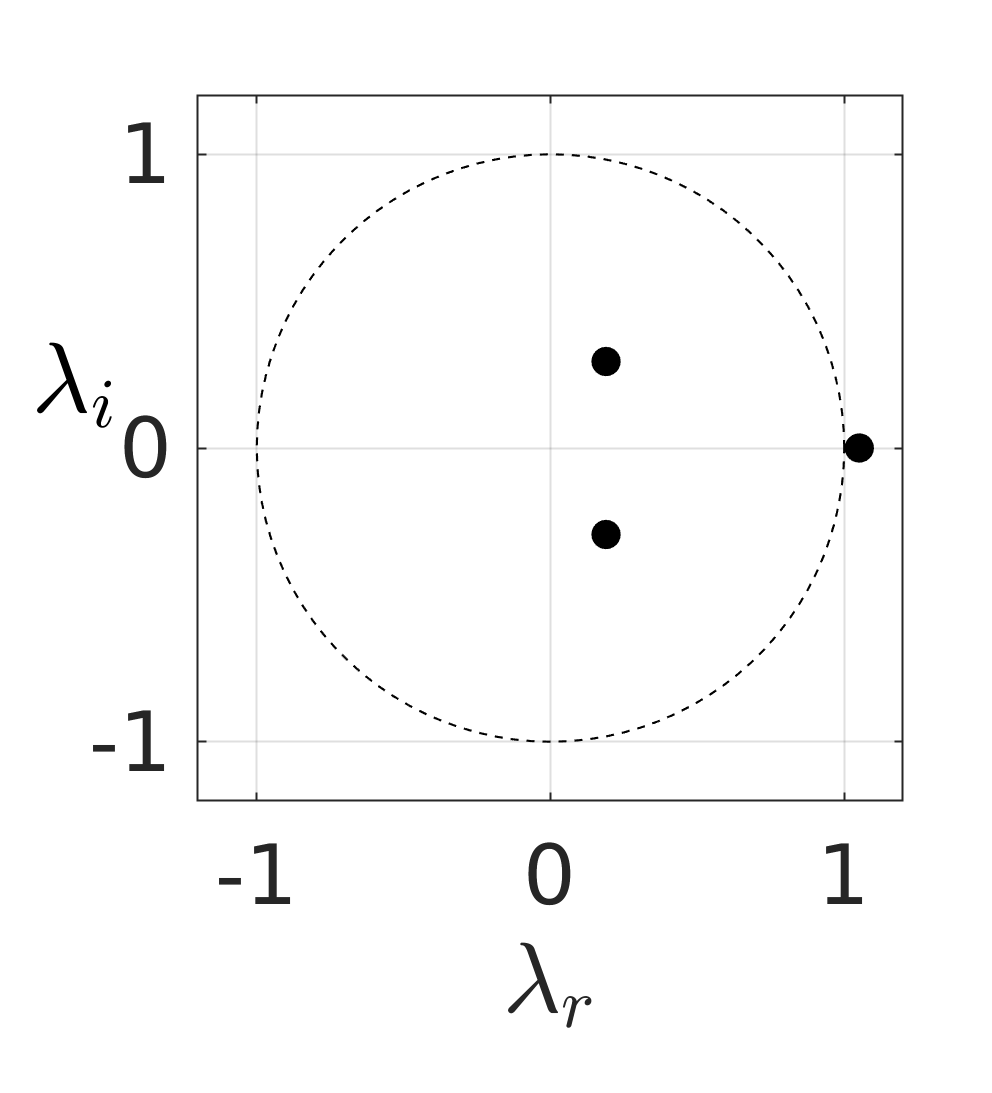
The multipliers of the other two periodic solutions : is shown in figure 26(right). The Floquet exponent of the leading multiplier is , equal to the growth rate at the fixed point .
|
 |
As a consequence, if the additional degree of freedom , introduced by the pitchfork bifurcation, do not couple, at the onset of the bifurcation, to the primary degrees of freedom associated with the Hopf bifurcation (see § 3.5), then it is easy to understand that both the symmetric steady solution and the statistically symmetric periodic solution , being the period of the limit cycle, will both undergo an instability with respect to the symmetry breaking provoked by the pitchfork bifurcation (). This simultaneous instability of both the symmetric fixed point and the statistically symmetric limit cycle looks like an instability of the subspace () with respect to the transverse direction , associated with the active degree of freedom introduced by the pitchfork bifurcation.
References
- Bansal & Yarusevych (2017) Bansal, M. S. & Yarusevych, S. 2017 Experimental study of flow through a cluster of three equally spaced cylinders. Exp. Thermal Fluid Sci. 80, 203–217.
- Barkley (2006) Barkley, D. 2006 Linear analysis of the cylinder wake mean flow. EPL (Europhysics Letters) 75 (5), 750.
- Barkley & Henderson (1996) Barkley, D. & Henderson, R. 1996 Three-dimensional floquet stability analysis of the wake of a circular cylinder. J. Fluid Mech. 322, 215–241.
- Bonnavion & Cadot (2018) Bonnavion, G. & Cadot, O. 2018 Unstable wake dynamics of rectangular flat-backed bluff bodies with inclination and ground proximity. J. Fluid Mech. 854, 196–232.
- Bourgeois et al. (2013) Bourgeois, J. A., Noack, B. R. & Martinuzzi, R. J. 2013 Generalised phase average with applications to sensor-based flow estimation of the wall-mounted square cylinder wake. J. Fluid Mech. 736, 316–350.
- Brunton & Noack (2015) Brunton, S. L. & Noack, B. R. 2015 Closed-loop turbulence control: Progress and challenges. Appl. Mech. Rev. 67 (5), 050801:01–48.
- Brunton et al. (2016) Brunton, S. L., Proctor, J. L. & Kutz, J. N. 2016 Discovering governing equations from data by sparse identification of nonlinear dynamical systems. Proc. Natl. Acad. Sci. 113 (5), 3932–3937.
- Cadot et al. (2015) Cadot, O., Evrard, A. & Pastur, L. 2015 Imperfect supercritical bifurcation in a three-dimensional turbulent wake. Phys. Rev. E 91 (6), 063005.
- Cornejo Maceda (2017) Cornejo Maceda, G. Y. 2017 Machine learning control applied to wake stabilization. MS2 Internship Report, LIMSI and ENSAM, Paris, France.
- Cross & Hohenberg (1993) Cross, M. C. & Hohenberg, P. C. 1993 Pattern formation outside of equilibrium. Rev. Mod. Phys. 65 (3), 851.
- Ding & Kawahara (1999) Ding, Y. & Kawahara, M. 1999 Three-dimensional linear stability analysis of incompressible viscous flows using the finite element method. Int. J. Num. Meth. Fluids 31 (2), 451–479.
- Fabre et al. (2008) Fabre, D., Auguste, F. & Magnaudet, J. 2008 Bifurcations and symmetry breaking in the wake of axisymmetric bodies. Phys. Fluids 20 (5), 051702.
- Fletcher (1984) Fletcher, C. A. 1984 Computational Galerkin Methods, 1st edn. New York: Springer.
- Gomez et al. (2016) Gomez, F., Blackburn, H. M., Rudman, M., Sharma, A. S. & McKeon, B. J. 2016 A reduced-order model of three-dimensional unsteady flow in a cavity based on the resolvent operator. J. Fluid Mech. 798, R2–1..14.
- Gorban & Karlin (2005) Gorban, A. N. & Karlin, I. V. 2005 Invariant Manifolds for Physical and Chemical Kinetics. Lecture Notes in Physics Vol. 660. Berlin: Springer-Verlag.
- Grandemange et al. (2012) Grandemange, M., Cadot, O. & Gohlke, M. 2012 Reflectional symmetry breaking of the separated flow over three-dimensional bluff bodies. Phys. Rev. E 86 (3), 035302.
- Grandemange et al. (2013) Grandemange, M., Gohlke, M. & Cadot, O. 2013 Turbulent wake past a three-dimensional blunt body. part 1. global modes and bi-stability. J. Fluid Mech. 722, 51–84.
- Grandemange et al. (2014) Grandemange, M., Gohlke, M. & Cadot, O. 2014 Statistical axisymmetry of the turbulent sphere wake. Exp. Fluids 55 (11), 1838.
- Gumowski et al. (2008) Gumowski, K., Miedzik, J., Goujon-Durand, S., Jenffer, P. & Wesfreid, J. E. 2008 Transition to a time-dependent state of fluid flow in the wake of a sphere. Phys. Rev. E 77 (5), 055308.
- Hopf (1948) Hopf, E. 1948 A mathematical example displaying features of turbulence. Commun. Pure Appl. Math. 1, 303–322.
- Ishar et al. (2019) Ishar, R., Kaiser, E., Morzynski, M., Albers, M., Meysonnat, P., Schröder, W. & Noack, B. R. 2019 Metric for attractor overlap. J. Fluid Mech. (in print).
- Jiménez (2018) Jiménez, J. 2018 Coherent structures in wall-bounded turbulence. J. Fluid Mech. 842.
- Jordan & Smith (1999) Jordan, D. W. & Smith, P. 1999 Nonlinear ordinary differential equations: an introduction to dynamical systems, , vol. 2. Oxford University Press, USA.
- Lam & Cheung (1988) Lam, K. & Cheung, W. C. 1988 Phenomena of vortex shedding and flow interference of three cylinders in different equilateral arrangements. J. Fluid Mech. 196, 1–26.
- Landau (1944) Landau, L. D. 1944 On the problem of turbulence. C.R. Acad. Sci. USSR 44, 311–314.
- Landau & Lifshitz (1987) Landau, L. D. & Lifshitz, E. M. 1987 Fluid Mechanics, 2nd edn. Course of Theoretical Physics Vol. 6. Oxford: Pergamon Press.
- Loiseau et al. (2018) Loiseau, J. C., Noack, B. R. & Brunton, S. L. 2018 Sparse reduced-order modeling: Sensor-based dynamics to full-state estimation. J. Fluid Mech. 844, 459–490.
- Luchtenburg et al. (2009) Luchtenburg, D. M., Günter, B., Noack, B. R., King, R. & Tadmor, G. 2009 A generalized mean-field model of the natural and actuated flows around a high-lift configuration. J. Fluid Mech. 623, 283–316.
- Malkus (1956) Malkus, W. V. R. 1956 Outline of a theory of turbulent shear flow. J. Fluid Mech. 1, 521–539.
- Manneville (2010) Manneville, P. 2010 Instabilities, chaos and turbulence, , vol. 1. World Scientific.
- Meliga et al. (2009) Meliga, P., Chomaz, J.-M. & Sipp, D. 2009 Global mode interaction and pattern selection in the wake of a disk: a weakly nonlinear expansion. J. Fluid Mech. 633, 159–189.
- Mittal (1999) Mittal, R. 1999 Planar symmetry in the unsteady wake of a sphere. AIAA J. 37 (3), 388–390.
- Morzynski et al. (1999) Morzynski, M., Afanasiev, K. & Thiele, F. 1999 Solution of the eigenvalue problems resulting from global non-parallel flow stability analysis. Comput. Methods. Appl. Mech. Engrg 169 (1), 161 – 176.
- Newhouse et al. (1978) Newhouse, S., Ruelle, D. & Takens, F. 1978 Occurrence of strange axiom A attractors near quasi periodic flows on , m 3. Commun. Math. Phys. 64 (1), 35–40.
- Noack (2016) Noack, B. R. 2016 From snapshots to modal expansions – bridging low residuals and pure frequencies. J. Fluid Mech. 802, 1–4.
- Noack et al. (2003) Noack, B. R., Afanasiev, K., Morzyński, M., Tadmor, G. & Thiele, F. 2003 A hierarchy of low-dimensional models for the transient and post-transient cylinder wake. J. Fluid Mech. 497, 335–363.
- Noack & Eckelmann (1994a) Noack, B. R. & Eckelmann, H. 1994a A global stability analysis of the steady and periodic cylinder wake. J. Fluid Mech. 270, 297–330.
- Noack & Eckelmann (1994b) Noack, B. R. & Eckelmann, H. 1994b Theoretical investigation of the bifurcations and the turbulence attractor of the cylinder wake. Z. angew. Math. Mech. 74 (5), T396–T397.
- Noack & Morzyński (2017) Noack, B. R. & Morzyński, M. 2017 The fluidic pinball — a toolkit for multiple-input multiple-output flow control (version 1.0). Tech. Rep. 02/2017. Chair of Virtual Engineering, Poznan University of Technology, Poland.
- Noack et al. (2008) Noack, B. R., Schlegel, M., Ahlborn, B., Mutschke, G., Morzyński, M., Comte, P. & Tadmor, G. 2008 A finite-time thermodynamics of unsteady fluid flows. J. Non-Equilibr. Thermodyn. 33, 103–148.
- Noack et al. (2016) Noack, B. R., Stankiewicz, W., Morzyński, M. & Schmid, P. J. 2016 Recursive dynamic mode decomposition of transient and post-transient wake flows. J. Fluid Mech. 809, 843–872.
- Price & Paidoussis (1984) Price, S. J. & Paidoussis, M. P. 1984 The aerodynamic forces acting on groups of two and three circular cylinders when subject to a cross-flow. J. Wind Eng. Indust. Aero. 17 (3), 329–347.
- Rempfer (1994) Rempfer, D. 1994 On the structure of dynamical systems describing the evolution of coherent structures in a convective boundary layer. Phys. Fluids 6 (3), 1402–4.
- Rempfer & Fasel (1994) Rempfer, D. & Fasel, H. F. 1994 Evolution of three-dimensional coherent structures in a flat-plate boundary-layer. J. Fluid Mech. 260, 351–375.
- Reynolds & Hussain (1972) Reynolds, W. C. & Hussain, A. K. M. F. 1972 The mechanics of an organized wave in turbulent shear flow. Part 3. Theoretical model and comparisons with experiments. J. Fluid Mech. 54, 263–288.
- Rigas et al. (2014) Rigas, G., Oxlade, A. R., Morgans, A. S. & Morrison, J. F. 2014 Low-dimensional dynamics of a turbulent axisymmetric wake. J. Fluid Mech. 755.
- Rigas et al. (2017) Rigas, G., Schmidt, O. T., Colonius, T. & Bres, G. A. 2017 One-way navier-stokes and resolvent analysis for modeling coherent structures in a supersonic turbulent jet. In 23rd AIAA/CEAS Aeroacoustics Conference, p. 11. Reston, VA, USA: AIAA - American Institute of Aeronautics and Astronautics, 23rd AIAA/CEAS Aeroacoustics Conference, Denver, CO, USA.
- Roweis & Saul (2000) Roweis, S. T. & Saul, L. K. 2000 Nonlinear dimensionality reduction by locally linear embedding. Science 290 (5500), 2323–2326.
- Rowley & Dawson (2017) Rowley, C. W. & Dawson, S. T. 2017 Model reduction for flow analysis and control. Ann. Rev. Fluid Mech. 49, 387–417.
- Rowley et al. (2009) Rowley, C. W., Mezić, I., Bagheri, S., Schlatter, P. & Henningson, D. S. 2009 Spectral analysis of nonlinear flows. J. Fluid Mech. 645, 115–127.
- Ruelle & Takens (1971) Ruelle, D. & Takens, F. 1971 On the nature of turbulence. Les rencontres physiciens-mathématiciens de Strasbourg-RCP25 12, 1–44.
- Sayers (1987) Sayers, A. T. 1987 Flow interference between three equispaced cylinders when subjected to a cross flow. J. Wind Eng. Indust. Aero. 26 (1), 1–19.
- Schatz et al. (1995) Schatz, M. F., Barkley, D. & Swinney, H. L. 1995 Instability in a spatially periodic open flow. Phys. Fluids 7 (2), 344–358.
- Schewe (1983) Schewe, G. 1983 On the force fluctuations acting on a circular cylinder in crossflow from subcritical up to transcritical Reynolds numbers. J. Fluid Mech. 133, 265–285.
- Schlegel & Noack (2015) Schlegel, M. & Noack, B. R. 2015 On long-term boundedness of galerkin models. J. Fluid Mech. 765, 325–352.
- Schmid (2010) Schmid, P. J. 2010 Dynamic mode decomposition for numerical and experimental data. J. Fluid Mech. 656, 5–28.
- Schumm et al. (1994) Schumm, M., Berger, E. & Monkewitz, P. A. 1994 Self-excited oscillations in the wake of two-dimensional bluff bodies and their control. J. Fluid Mech. 271, 17–53.
- Sipp & Lebedev (2007) Sipp, D. & Lebedev, A. 2007 Global stability of base and mean flows: a general approach and its applications to cylinder and open cavity flows. J. Fluid Mech. 593 (1), 333–358.
- Strogatz et al. (1994) Strogatz, S., Friedman, M., Mallinckrodt, A. J. & McKay, S. 1994 Nonlinear dynamics and chaos: with applications to physics, biology, chemistry, and engineering. Computers Phys. 8 (5), 532–532.
- Strykowski & Sreenivasan (1990) Strykowski, P. J. & Sreenivasan, K. R. 1990 On the formation and suppression of vortex ‘shedding’ at low reynolds numbers. J. Fluid Mech. 218, 71–107.
- Stuart (1958) Stuart, J. T. 1958 On the non-linear mechanics of hydrodynamic stability. J. Fluid Mech. 4, 1–21.
- Swift & Hohenberg (1977) Swift, J. & Hohenberg, P. C. 1977 Hydrodynamic fluctuations at the convective instability. Phys. Rev. A 15 (1), 319.
- Szaltys et al. (2012) Szaltys, P., Chrust, M., Przadka, A., Goujon-Durand, S., Tuckerman, L. S. & Wesfreid, J. E. 2012 Nonlinear evolution of instabilities behind spheres and disks. J. Fluids Struct. 28, 483–487.
- Tadmor et al. (2011) Tadmor, G., Lehmann, O., Noack, B. R., Cordier, L., Delville, J., Bonnet, J.-P. & Morzyński, M. 2011 Reduced order models for closed-loop wake control. Philos. Trans. R. S. A 369 (1940), 1513–1524.
- Taira et al. (2017) Taira, K., Brunton, S. L., Dawson, S. T., Rowley, C. W., Colonius, T., McKeon, B. J., Schmidt, O. T., Gordeyev, S., Theofilis, V. & Ukeiley, L. S. 2017 Modal analysis of fluid flows: An overview. AIAA J. pp. 4013–4041.
- Tatsuno et al. (1998) Tatsuno, M., Amamoto, H. & Ishi-i, K. 1998 Effects of interference among three equidistantly arranged cylinders in a uniform flow. Fluid Dyn. Res. 22 (5), 297.
- Taylor & Hood (1973) Taylor, C. & Hood, P. 1973 A numerical solution of the navier-stokes equations using the finite element technique. Comput. Fluids 1, 73–100.
- Turton et al. (2015) Turton, S. E., Tuckerman, L. S. & Barkley, D. 2015 Prediction of frequencies in thermosolutal convection from mean flows. Phys. Rev. E 91 (4), 043009.
- Watson (1960) Watson, J. 1960 On the non-linear mechanics of wave disturbances in stable and unstable parallel flows. Part 2. the development of a solution for plane Poiseuille flow and for plane Couette flow. J. Fluid Mech. 9, 371–389.
- Zaitsev & Shliomis (1971) Zaitsev, V. M. & Shliomis, M. I. 1971 Hydrodynamic fluctuations near convection threshold. Sov. Phys. JETP 32, 866.
- Zhang et al. (1994) Zhang, H.-Q., Noack, B. R. & Eckelmann, H. 1994 Numerical computation of the 3-d cylinder wake. Tech. Rep. 3/1994. Max-Planck-Institut für Strömungsforschung, Göttingen, Germany.