Block clustering of Binary Data with Gaussian Co-variables

Abstract

The simultaneous grouping of rows and columns is an important technique that is increasingly used in large-scale data analysis. In this paper, we present a novel co-clustering method using co-variables in its construction. It is based on a latent block model taking into account the problem of grouping variables and clustering individuals by integrating information given by sets of co-variables. Numerical experiments on simulated data sets and an application on real genetic data highlight the interest of this approach.

1 Introduction

Classification is a method of data analysis that aims to group together a set of observations into homogeneous classes. It plays an increasingly important role in many scientific and technical fields. Its aim is the automatic resolution of problems by decision-making based on the observations and to define the rules for classifying objects depending on qualitative or quantitative variables.

Clustering is the most popular technique for data analysis in many disciplines. In recent years, co-clustering has been increasingly used. Unlike classical clustering, which groups similar objects from a single collection of objects, co-clustering or bi-clustering [1] aims at simultaneously grouping objects from two disjoint sets, thus revealing interactions between elements of two sets.

It is most often used with bipartite spectral graphing partitioning methods in the field of extracting text data [2] by simultaneously grouping documents and content (words) and analyzing huge corpora unlabeled documents [3] to simultaneously understand aggregates of subsets of web users sessions and information from the page views. Co-clustering algorithms have also been developed for computer vision applications. It is used for grouping images simultaneously with their low-level visual characteristics and for content-based search [4].

In this paper we extend co-clustering methods allowing simultaneous detection of associations between variables and individuals by taking into account co-variables. These co-variables can be additional measures of interest. Consideration of a co-variable is expected to provide better separation of groups of variables and especially groups of individuals. Classification quality is determined by general validation measures specific to the co-clustering method. This approach can be useful when co-clustering a set $\mathbf{X}$ of variables and individuals in coherence with an independent $\mathbf{Y}$ variable measured on these same individuals. For example, in the co-clustering of several SNP (Single-Nucleotide Polymorphism) variables on different patients with respect to a measured phenotype (see application in section 3).

The paper is organized as follows. In the first part, we explain the principle of block mixture models through section 2. The latent block model for binary variable takes into account co-variables and the model parameters estimation is proposed in Section 2.2. The parameter estimation method is described in section 2.3. The choice of the optimal number of blocks and the measure of influence of each variable on the co-variable $\mathbf{Y}$ is presented in the second part (section 2.5 and 2.6). The method is illustrated on simulated and real genetic data in the last part (section 3).

2 Block mixture models

2.1 Classical latent block model

Let $\mathbf{x}$ be a data set doubly indexed by a set $I$ with $n$ elements (individuals) and a set $J$ with $m$ elements (variables). We represent a partition of $I$ into $g$ clusters by $\mathbf{z}=(z_{11},\ldots,z_{ng})$ with $z_{ik}=1$ if $i$ belongs to cluster $k$ and $z_{ik}=0$ otherwise, $z_{i}=k$ if $z_{ik}=1$ and we denote by $z_{.k}=\sum_{i}z_{ik}$ the cardinality of row cluster $k$. Similarly, we represent a partition of $J$ into $d$ clusters by $\mathbf{w}=(w_{11},\ldots,w_{md})$ with $w_{j\ell}=1$ if $j$ belongs to cluster $\ell$ and $w_{j\ell}=0$ otherwise, $w_{j}=\ell$ if $w_{j\ell}=1$ and we denote $w_{.\ell}=\sum_{j}w_{j\ell}$ the cardinality of column cluster $\ell$.

The block mixture model formulation is defined in [5] and [6] (among others) by the following probability density function

$$f(\mathbf{x};\boldsymbol{\theta})=\sum_{\mathbf{u}\in{\cal U}}p(\mathbf{u};\boldsymbol{\theta})f(\mathbf{x}|\mathbf{u};\boldsymbol{\theta})$$

where ${\cal U}$ denotes the set of all possible labels of $I\times J$ and $\boldsymbol{\theta}$ contains all the unknown parameters of this model. By restricting this model to a set of labels of $I\times J$ defined by a product of labels of $I$ and $J$, and further assuming that the labels of $I$ and $J$ are independent of each other, one obtain the decomposition

$$f(\mathbf{x};\boldsymbol{\theta})=\sum_{(\mathbf{z},\mathbf{w})\in\cal{Z\times W}}p(\mathbf{z};\boldsymbol{\theta})p(\mathbf{w};\boldsymbol{\theta})f(\mathbf{x}|\mathbf{z},\mathbf{w};\boldsymbol{\theta})$$ (1)

where ${\cal Z}$ and ${\cal W}$ denote the sets of all possible labellings $\mathbf{z}$ of $I$ and $\mathbf{w}$ of $J$. Equation (1) define a Latent Block Model (LBM).

2.2 LBM for binary variables with co-variables: General formulation

From now, we assume that $\mathbf{x}$ is a binary data set. Let $\mathbf{y}$ represents a data-set (co-variables) of $\mathbb{R}^{p}$ indexed by $I$. In order to take into account this set of co-variables the classical block model formulation is extended to propose a block mixture model defined by the following probability density function

$$f(\mathbf{x},\mathbf{y};\boldsymbol{\theta})=\sum_{(\mathbf{z},\mathbf{w})\in\cal{Z\times W}}p(\mathbf{z};\boldsymbol{\theta})p(\mathbf{w};\boldsymbol{\theta})f(\mathbf{x}|\mathbf{y},\mathbf{z},\mathbf{w};\boldsymbol{\theta})f(\mathbf{y}|\mathbf{z};\boldsymbol{\theta}).$$ (2)

By extending the latent class principle of local independence to our block model, each data pair $(x_{ij},\mathbf{y}_{i})$ will be independent once $z_{i}$ and $w_{j}$ are fixed. Hence we have

$$f(\mathbf{x},\mathbf{y}|\mathbf{z},\mathbf{w};\boldsymbol{\theta})=\prod_{i,j}f(x_{ij},\mathbf{y}_{i}|\mathbf{z}_{i},\mathbf{w}_{j};\boldsymbol{\theta}).$$

We choose to model the dependency between $x_{ij}$ and $\mathbf{y}_{i}$ using the canonical link for binary response data

$$f(x_{ij}|\mathbf{y}_{i},\boldsymbol{\beta}_{z_{i}w_{j}})=\operatorname{logis}(\beta_{0,z_{i}w_{j}}+\boldsymbol{\beta}_{z_{i}w_{j}}^{T}\mathbf{y}_{i})^{x_{ij}}\,\left(1-\operatorname{logis}(\beta_{0,z_{i}w_{j}}+\boldsymbol{\beta}_{z_{i}w_{j}}^{T}\mathbf{y}_{i})\right)^{1-{x_{ij}}}$$ (3)

with $(\beta_{0},\boldsymbol{\beta}_{k,l})\in\mathbb{R}^{p+1}$ and $\operatorname{logis}(x)=e^{x}/(1+e^{x})$. Each data point $\mathbf{y}_{i}$ will be independent once $z_{i}$ are fixed. In the examples presented in section 3, we choose

$$f(\mathbf{y}|\mathbf{z};\boldsymbol{\theta})=\prod_{i}\phi(\mathbf{y}_{i};\boldsymbol{\mu}_{z_{i}},\boldsymbol{\Sigma}_{z_{i}})$$

with $\phi$ denoting the multivariate Gaussian density in $\mathbb{R}^{p}$.

In order to simplify the notation, we add a constant coordinate $1$ to vectors $\mathbf{y}_{i}$ and write $\boldsymbol{\beta}_{k,l}$ in the latter rather than $(\beta_{0,k,l},\boldsymbol{\beta}_{k,l})$.

The parameters are thus $\boldsymbol{\theta}=(\boldsymbol{\pi},\boldsymbol{\rho},\boldsymbol{\beta},\boldsymbol{\mu},\boldsymbol{\Sigma})$, where $\boldsymbol{\pi}=(\pi_{1},\ldots,\pi_{g})$, $\boldsymbol{\rho}=(\rho_{1},\ldots,\rho_{d})$ are the vectors of probabilities $\pi_{k}$ and $\rho_{\ell}$ that a row and a column belong to the $k$th row component and to the $\ell$th column component respectively, $\boldsymbol{\beta}=(\boldsymbol{\beta}_{kl})$ are the coefficients of the logistic function, $\boldsymbol{\mu}$ and $\boldsymbol{\Sigma}$ are the means and variances of the Gaussian density. In summary, we obtain the latent block mixture model with pdf

$$f(\mathbf{x},\mathbf{y}|\boldsymbol{\theta})=\sum_{(\mathbf{z},\mathbf{w})\in{\cal Z}\times{\cal W}}\prod_{i,j}\pi_{z_{i}}\rho_{w_{j}}\operatorname{logis}(\mathbf{y}_{i}^{T}\boldsymbol{\beta}_{z_{i}w_{j}})^{x_{ij}}\left(1-\operatorname{logis}(\mathbf{y}_{i}^{T}\boldsymbol{\beta}_{z_{i}w_{j}})\right)^{1-x_{ij}}\phi(\mathbf{y}_{i};\boldsymbol{\mu}_{z_{i}},\boldsymbol{\Sigma}_{z_{i}}).$$ (4)

Using the above expression, the randomized data generation process can be described by the four steps row labellings (R), column labellings (C), co-variable data generation (Y) and data generation (X) as follows:

1. Generate the labellings $\mathbf{z}=(z_{1},\ldots,z_{n})$ according to the distribution $\boldsymbol{\pi}=(\pi_{1},\ldots,\pi_{g})$.

2. Generate the labellings $\mathbf{w}=(w_{1},\ldots,w_{m})$ according to the distribution $\boldsymbol{\rho}=(\rho_{1},\ldots,\rho_{d})$.

3. Generate for $i=1,...,n$ vector $\mathbf{y}_{i}$ according to the Gaussian distribution $\mathcal{N}_{p}(\boldsymbol{\mu}_{z_{i}},\boldsymbol{\Sigma}_{z_{i}})$.

4. Generate for $i=1,...,n$ and $j=1,...,m$ a value $x_{ij}$ according to the Bernoulli distribution $f(x_{ij}|\mathbf{y}_{i};\boldsymbol{\beta}_{z_{i}w_{j}})$ given in (3).

2.3 Model Parameters Estimation

The complete data is represented as a vector $(\mathbf{x},\mathbf{y},\mathbf{z},\mathbf{w})$ where unobservable vectors $\mathbf{z}$ and $\mathbf{w}$ are the labels. The log-likelihood to maximize is

$$l(\boldsymbol{\theta})=\log f(\mathbf{x},\mathbf{y};\boldsymbol{\theta})$$ (5)

and the double missing data structure, namely $\mathbf{z}$ and $\mathbf{w}$, makes statistical inference more difficult than usual. More precisely, if we try to use an EM algorithm as in standard mixture model [7] the complete data log-likelihood is found to be

$$L_{C}(\mathbf{z},\mathbf{w},\boldsymbol{\theta})=\sum_{k}z_{.k}\log\pi_{k}+\sum_{\ell}w_{.\ell}\log\rho_{\ell}+\sum_{i,j,k,\ell}z_{ik}w_{j\ell}\log f(x_{ij},\mathbf{y}_{i};\boldsymbol{\theta}_{k\ell}).$$ (6)

The EM algorithm maximizes the log-likelihood $l(\boldsymbol{\theta})$ iteratively by maximizing the conditional expectation $Q(\boldsymbol{\theta},\boldsymbol{\theta}^{(c)})$ of the complete data log-likelihood given a previous current estimate $\boldsymbol{\theta}^{(c)}$ and $(\mathbf{x},\mathbf{y})$:

$$Q(\boldsymbol{\theta},\boldsymbol{\theta}^{(c)})=\mathbb{E}\left[L_{C}(\mathbf{z},\mathbf{w},\theta)\left|{\mathbf{x},\mathbf{y},\boldsymbol{\theta}^{(c)}}\right.\right]=\sum_{i,k}t_{ik}^{(c)}\log\pi_{k}+\sum_{j,\ell}r_{j\ell}^{(c)}\log\rho_{\ell}+\sum_{i,j,k,\ell}e_{ikj\ell}^{(c)}\log f(x_{ij},\mathbf{y}_{i};\boldsymbol{\theta}_{k\ell})$$

where

$$t_{ik}^{(c)}=P(z_{ik}=1|\mathbf{x},\mathbf{y},\boldsymbol{\theta}^{(c)}),\qquad r_{jl}^{(c)}=P(w_{j\ell}=1|\mathbf{x},\mathbf{y},\boldsymbol{\theta}^{(c)}),\qquad e_{ikj\ell}^{(c)}=P(z_{ik}w_{j\ell}=1|\mathbf{x},\mathbf{y},\boldsymbol{\theta}^{(c)})$$

Unfortunately, difficulties arise due to the dependence structure in the model, in particular to determine $e_{ikj\ell}^{(c)}$. The assumed independence of $\mathbf{z}$ and $\mathbf{w}$ in (1) is not conserved by the posterior probability.

To solve this problem an approximate solution is proposed in [5] using the [8] and [9] interpretation of the VEM algorithm. Consider a family of probability distribution $q(z_{ik},w_{j\ell})$ verifying $q(z_{ik},w_{j\ell})>0$ and the relation $q(z_{ik},w_{j\ell})=q(z_{ik})q(w_{j\ell})$, for all $i,j,k,l$. Set $t_{ik}=q(z_{ik})$ and $r_{jl}=q(w_{j\ell})$, $\mathbf{t}=(t_{ik})_{ik}$ for $i=1,\ldots,n$, $k=1,\ldots,g$ and $\mathbf{r}=(r_{jl})_{jl}$ for $j=1,\ldots,m$ and $l=1,\ldots,d$. One shows easily that

$$l(\boldsymbol{\theta})=\tilde{F}_{C}(\mathbf{t},\mathbf{r};\boldsymbol{\theta})+KL(q(\mathbf{z},\mathbf{w})\parallel p(\mathbf{z},\mathbf{w}|\mathbf{x},\mathbf{y},\boldsymbol{\theta}))$$ (7)

with $KL(q\parallel p)$ denoting the Kullback-Liebler divergence of distribution $p$ and $q$,

$$\tilde{F}_{C}(\mathbf{t},\mathbf{r};\boldsymbol{\theta})=\sum_{k}t_{.k}\log\pi_{k}+\sum_{\ell}r_{.\ell}\log\rho_{l}+\sum_{i,j,k,\ell}t_{ik}r_{j\ell}\log f(x_{ij},\mathbf{y}_{i};\boldsymbol{\theta}_{k\ell})+H(\mathbf{t})+H(\mathbf{r})$$ (8)

and $H(\mathbf{t})$, $H(\mathbf{r})$ denoting the entropy of $\mathbf{t}$ and $\mathbf{r}$, i.e.

$$H(\mathbf{t})=\sum_{ik}t_{ik}\log t_{ik},\qquad H(\mathbf{r})=\sum_{jl}r_{jl}\log r_{jl}.$$

$\tilde{F}_{C}$ is called the free energy or the fuzzy criterion. As the Kullback-Liebler divergence is always positive, the fuzzy criterion is a lower bound of the log-likelihood and is used as a replacement for it. Doing that, the maximization of the likelihood $l(\boldsymbol{\theta})$ is replaced by the following problem

$$\mathop{\mathrm{argmax}}_{\mathbf{t},\mathbf{r},\boldsymbol{\theta}}\tilde{F}_{C}(\mathbf{t},\mathbf{r},\boldsymbol{\theta}).$$

This maximization can be achieved using the BEM algorithm detailed hereafter.

2.4 Block expectation maximization (BEM) Algorithm

The fuzzy clustering criterion given in (8) can be maximized using a variational EM algorithm (VEM). We here outline the various expressions evaluated during E and M steps.

E-Step:

we compute either the values of $\mathbf{t}$ (respectively $\mathbf{r}$) with $\mathbf{r}$ (respectively $\mathbf{t}$) and $\boldsymbol{\theta}$ fixed (formulas (12), (13) hereafter). Details are given in appendix A.

M-Step:

we calculate row proportions $\boldsymbol{\pi}$ and column proportions $\boldsymbol{\rho}$. The maximization of $\tilde{F}_{C}$ w.r.t. $\boldsymbol{\pi}$, and w.r.t $\boldsymbol{\rho}$, is obtained by maximizing $\sum_{k}t_{.k}\log\pi_{k}$, and $\sum_{\ell}r_{.\ell}\log\rho_{\ell}$ respectively, which leads to

$$\pi_{k}=\frac{t_{.k}}{n}\quad\textrm{ and }\quad\rho_{\ell}=\frac{r_{.\ell}}{m}.$$ (9)

Also, for $\mathbf{t}$, $\mathbf{r}$ fixed, the estimate of model parameters $\boldsymbol{\beta}$ will be obtained by maximizing

$$\boldsymbol{\beta}_{kl}=\mathop{\mathrm{argmax}}_{\boldsymbol{\beta}}\sum_{ij}t_{ik}r_{jl}\log f(x_{ij}|\mathbf{y}_{i};\boldsymbol{\beta}),\quad k=1,\ldots,g,\quad l=1,\ldots,d.$$ (10)

Detail are given in appendix B. Finally parameters of the Gaussian density are given by the usual formulas

$$\boldsymbol{\mu}_{k}=\frac{1}{t_{.k}}\sum_{i}t_{ik}\mathbf{y}_{i}\qquad\mbox{ and }\qquad\boldsymbol{\Sigma}_{k}=\frac{1}{t_{.k}}\sum_{i}t_{ik}(\mathbf{y}_{i}-\boldsymbol{\mu}_{k})(\mathbf{y}_{i}-\boldsymbol{\mu}_{k})^{T}.$$ (11)

Putting everything together, we obtain the BEM algorithm.

BEM algorithm:

Using the E and M steps defined above, BEM algorithm can be enumerated as follows:

Initialization

Set $\mathbf{t}^{(0)},\mathbf{r}^{(0)}$ and $\boldsymbol{\theta}^{(0)}=(\boldsymbol{\pi}^{(0)},\boldsymbol{\rho}^{(0)},\boldsymbol{\beta}^{(0)},\boldsymbol{\mu}^{(0)}$, $\boldsymbol{\Sigma}^{(0)}).$

(a) Row-EStep

Compute $\mathbf{t}^{(c+1)}$ using formula

$$t_{ik}^{(c+1)}=\displaystyle\frac{\pi_{k}^{(c)}\displaystyle\prod_{jl}\left(f(x_{ij}|\mathbf{y}_{i};\boldsymbol{\beta}_{kl}^{(c)})\phi(\mathbf{y}_{i};\boldsymbol{\mu}_{k}^{(c)},\boldsymbol{\Sigma}_{k}^{(c)})\right)^{r_{jl}^{(c)}}}{\sum_{k}\pi_{k}^{(c)}\displaystyle\prod_{jl}\left(f(x_{ij}|\mathbf{y}_{i};\boldsymbol{\beta}_{kl}^{(c)})\phi(\mathbf{y}_{i};\boldsymbol{\mu}_{k}^{(c)},\boldsymbol{\Sigma}_{k}^{(c)})\right)^{r_{jl}^{(c)}}}.$$ (12)

(b) Row-MStep

Compute $\boldsymbol{\pi}^{(c+1)}$, $\boldsymbol{\mu}^{(c+1)}$, $\boldsymbol{\Sigma}^{(c+1)}$ using equations (9) and (11) and estimate $\boldsymbol{\beta}^{(c+1/2)}$ by solving maximization problem (10).

(c) Col-EStep

Compute $\mathbf{r}^{(c+1)}$ using formula

$$r_{jl}^{(c+1)}=\frac{\rho_{l}^{(c)}\displaystyle\prod_{ik}f(x_{ij}|\mathbf{y}_{i};\boldsymbol{\beta}_{kl}^{(c+1/2)})^{t_{ik}^{(c+1)}}}{\sum_{l}\rho_{l}^{(c)}\displaystyle\prod_{ik}f(x_{ij}|\mathbf{y}_{i};\boldsymbol{\beta}_{kl}^{(c+1/2)})^{t_{ik}^{(c+1)}}}.$$ (13)

Observe that $r_{jl}$ does not depend of the density of $\mathbf{y}$.

(d) Col-MStep

Compute $\boldsymbol{\rho}^{(c+1)}$ using equations (9) and estimate $\boldsymbol{\beta}^{(c+1)}$ by solving maximization problem (10).

Iterate

Iterate (a)-(b)-(c)-(d) until convergence.

2.5 Selecting the number of blocks

BIC is an information criterion defined as an asymptotic approximation of the logarithm of the integrated likelihood ([10]). The standard case leads to write BIC as a penalised maximum likelihood:

$$\mathrm{BIC}=-2\max_{\boldsymbol{\theta}}l(\boldsymbol{\theta})+D\log(N)$$

where $N$ is the number of statistical units and $D$ the number of free parameters and $l(\boldsymbol{\theta})$ defined in (5). Unfortunately, this approximation cannot be used for LBM, due to the dependency structure of the observations $(\mathbf{x},\mathbf{y})$. However, a heuristic have been stated to define BIC in [11] and [12]. BIC-like approximations ICL lead to the following approximation as $n$ and $m$ tend to infinity

$$\mathrm{BIC}(g,d)=-2\max_{\boldsymbol{\theta}}\log f(\mathbf{x},\mathbf{y};\boldsymbol{\theta})+(g-1)\log n+\lambda\log n+(d-1)\log m+gd(p+1)\log(mn)$$ (14)

with $\lambda$ the number of parameters of the $\mathbf{y}$ distribution. For LBM, the intractable likelihood $f(\mathbf{x},\mathbf{y};\boldsymbol{\theta})$ is replaced by the maximized free energy $\tilde{F}_{C}$ in (8) obtained by the BEM algorithm.

2.6 Measuring Influence of a Variable

Let $j$ be fixed (a column of the matrix $\mathbf{x}$). We would like to measure the effect of the variable $\mathbf{x}^{j}=(x_{ij})_{i=1}^{n}$ on $\mathbf{y}$. It is possible to obtain a measure of this effect by looking to the posterior probability of $\mathbf{y}$.

Lemma 1

Let $(\mathbf{x},\mathbf{z},\mathbf{w})$ fixed. For $l=1,\ldots,d$ let $m_{l}$ denotes the number of columns with label $l$, i.e $m_{l}=\#\{w_{jl}=1,\;j=1,\ldots m\}$ and for a row $i$ fixed let $m_{il}$ denotes the number of elements such that ${w_{jl}=1}$ and $x_{ij}=1$, i.e. $m_{il}=\#\{w_{jl}x_{ij}=1,\;j=1,\ldots n\}$. The posterior probability of the co-variable $\mathbf{y}$ is

$$f(\mathbf{y}|\mathbf{x},\mathbf{z},\mathbf{w},\boldsymbol{\theta}) \propto\prod_{i=1}^{n}\prod_{l=1}^{d}\pi_{z_{i}}\rho_{l}^{n_{l}}\operatorname{logis}(\mathbf{y}_{i}^{T}\boldsymbol{\beta}_{z_{i}l})^{n_{il}}\left(1-\operatorname{logis}(\mathbf{y}_{i}^{T}\boldsymbol{\beta}_{z_{i}l})\right)^{m_{l}-m_{il}}\phi(\mathbf{y}_{i};\boldsymbol{\mu}_{z_{i}},\boldsymbol{\Sigma}_{z_{i}})$$

$$\propto\prod_{i=1}^{n}\pi_{z_{i}}\phi(\mathbf{y}_{i};\boldsymbol{\mu}_{z_{i}},\boldsymbol{\Sigma}_{z_{i}})\prod_{l=1}^{d}\rho_{l}^{n_{l}}\frac{e^{n_{il}\mathbf{y}_{i}^{T}\boldsymbol{\beta}_{z_{i}l}}}{\left(1+e^{\mathbf{y}_{i}^{T}\boldsymbol{\beta}_{z_{i}l}}\right)^{m_{l}}}$$ (15)

Alternatively, for $k=1,\ldots,g$, let $n_{k}$ denotes the number of rows with label $k$, i.e. $n_{k}=\#\{z_{ik}=1,i=1,\ldots,m\}$. The posterior probability of the co-variable $\mathbf{y}$ is

$$f(\mathbf{y}|\mathbf{x},\mathbf{z},\mathbf{w},\boldsymbol{\theta})\propto\prod_{j=1}^{m}\rho_{w_{j}}\prod_{k=1}^{g}\pi_{k}^{m_{j}}\prod_{i:z_{i}=k}\operatorname{logis}(\mathbf{y}_{i}^{T}\boldsymbol{\beta}_{kw_{j}})^{x_{ij}}\left(1-\operatorname{logis}(\mathbf{y}_{i}^{T}\boldsymbol{\beta}_{kw_{j}})\right)^{1-x_{ij}}\phi(\mathbf{y}_{i};\boldsymbol{\mu}_{k},\boldsymbol{\Sigma}_{k}).$$ (16)

The proof of this lemma is straightforward and therefore omitted.

Assuming $\mathbf{z}$ and $\mathbf{w}$ known, we measure the influence of a variable using its contribution to the posterior probability. Fixing $j$, taking the logarithm and eliminating terms independent of $\mathbf{x}^{j}$, we obtain the influence measure criteria

$$I(j) =\log\rho_{w_{j}}+\sum_{i=1}^{n}{x_{ij}}\log\operatorname{logis}(\mathbf{y}_{i}^{T}\boldsymbol{\beta}_{z_{i}w_{j}})+\sum_{i=1}^{n}{(1-x_{ij})}\log\left(1-\operatorname{logis}(\mathbf{y}_{i}^{T}\boldsymbol{\beta}_{z_{i}w_{j}})\right)$$

$$=\log\rho_{w_{j}}+\sum_{i=1}^{n}\left(x_{ij}\mathbf{y}_{i}^{T}\boldsymbol{\beta}_{z_{i}w_{j}}-\log({1+\exp(\mathbf{y}_{i}^{T}.\boldsymbol{\beta}_{z_{i}w_{j}})})\right)$$ (17)

which is interpreted as the $\log$-contribution to the posterior distribution (16) of the variable $\mathbf{x}^{j}$. Replacing the unknown labels $w_{j}$ and $z_{i}$ by their MAP estimators $\hat{w}_{j}$ and $\hat{z}_{i}$, we are able to sort the variables from the most to the less influential.

3 Examples

3.1 Simulated data

3.1.1 Computational time

We compute 80 times the elapsed time of the model for various configurations of the parameter on a HP Zbook G3. The (averaged) computing time as a function of $m$ when $g=2$ for different values of $m$ (the number of columns) and when $d$ (the number of cluster in columns) take values 2 and 6 is plotted in figure 1 below

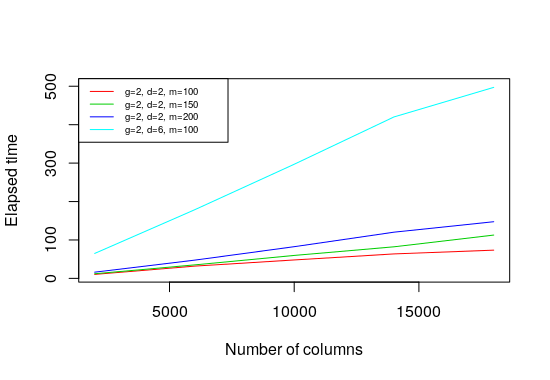
Figure 1: computational elapsed time for $n=$ 2000, 6000, 10000, 14000 and 18000 (in minutes) and for various values of $m$.

We can observe that as $n$ grows the elapsed time grows linearly, but that the slope increases as $d$ (the number of class in columns) is increased.

3.1.2 Error rate

Next we simulate 80 times the number of columns well classified when $g=2$ and for various configurations of $m$ and $d$. The cluster of a column is estimated using the maximum a posterior (MAP) estimator

$$\hat{w}_{j}=\arg\max_{l=1}^{d}r_{jl}.$$

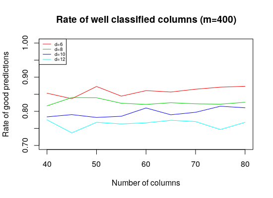
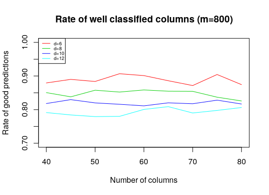
Figure 2: Rates of well classified columns when the number of rows is 400 and 800. The number of columns is between 40 and 80. The number of cluster is between 6 and 12. There is only two groups of rows.

From these partial results, we see that the number of bad classified columns labels increases as $d$ increases while it remains relatively constant with $m$. An other salient feature is that when the number of individuals ($n$) is greater, this error rate is lower. The number of well classified rows is stable near 0.9 for all tested configurations of the parameters and is not displayed.

3.2 Real Data Analysis

Here, we study data from an epidemiological and genetic survey of malaria disease in Senegal. Data were collected between 1990 to 2008. We worked on a dataset including $n=885$ individuals with measured malaria risk score (phenotype) and genotype available on several candidate genes for susceptibility/resistance to the disease. A total of $m=45$ Single Nucleotide Polymorphisms (SNPs) was considered across these genes and was used as genetic variables. The malaria risk score was a quantitative measure normally distributed and was considered as a co-variable for this co-clustering method. The SNPs are coded in dominant effect on the disease risk. Using the BIC criteria (see graph 3), we choose to focus on the model $d=2$ groups of individuals and $g=11$ groups of SNPs.

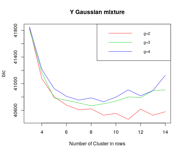
Figure 3: BIC computation for different values of $d$ and $g$. We observe that it is minimal for $g=2$ and $d=11$ among tested $d$ values $(1,\ldots,4)$ and $g$ values $(2,34)$ .

3.2.1 Analysis for phenotype data

The choice of a mixture model or not depends on the application context. In the case of genetic data, we are often interested in the comparison of the susceptible and the resistant to a given phenotype. In this application, we look for genes to explain the difference between susceptible and resistant which justifies the use of a mixture model on the target variable. After block-clustering, we find that the individuals are divided in two groups: the susceptibility category composed of a group of individuals with a value of phenotype essentially greater than zero and the resistant category composed of a group of individuals with a value of phenotype essentially less than zero (see figure 4).

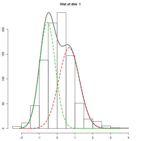
(a)

(b)

Figure 4: (a) - Empirical Distribution of the phenotype (histogram) - Distribution of the susceptible (red) - distribution of the resistant (green) - mixing distribution (grey).      (b) Array with the presence/absence of mutations before and after block-clustering

Observe how the marginal distribution of the phenotype, which is uni-modal, becomes multi-modal when conditioned by ($\mathbf{x},\mathbf{z}$).

3.2.2 Analysis for genotypes data

We looked at the SNPs to determine which ones would potentially be involved in malaria susceptibility / resistance.

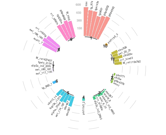
Figure 5: Representation of each block variable according to the influence measure

The proposed methodology allowed the selection of the most significant SNPs according to the influence measure proposed in section 2.6. The most frequent SNPs are grouped into the following classes: class 1 and 9. It is noted that the SNPs of these classes have been shown in the literature to have a high significance effect on malaria. Most G6P and hemoglobin SNPs are grouped into these 2 classes. Reviews from exiting literature gives us: Glucose-6-phosphate dehydrogenase (G6PD) deficiency is prevalent in sub-Saharan African populations and has been associated with protection against severe malaria [13, 14, 15, 16]. Studies above haplotype analysis reveal that the G6PD locus is an under-balanced selection, suggesting a malaria protection mechanism based on modest frequency alleles and avoiding parasite attachment [14]. Hemoglobins S and C (HbS and HbC respectively) are known to be two structurally variant forms of normal adult hemoglobin (HbA) resulting from distinct mutations in the $\beta$-globin gene. The protective effect of HbS against Plasmodium falciparum malaria has been shown by several authors [17, 18, 19]. In the case of HbC, the protection is highest in homozygous individuals with HbCC. The proposed model confirmed the strong link between sickle cell polymorphism (HBS), blood group ABO (HBC) and falciparum malaria in the West African population.

3.2.3 Association between phenotype and genotypes

The most common approach used in genetic data is the GWAS method (Genome Wide Association Studies). This method makes a linear regression of the quantitative phenotype on each genotype variable. By applying co-clustering with the phenotype as co-variable, we could obtain a dichotomy of the phenotype. This dichotomy allows us to divide individuals into two categories: susceptible and resistant. In this part, we compare the results of GWAS studies between the quantitative phenotype, the binary phenotype ($\mathbf{1}_{y_{i}\leq 0}$) and the (co-)clustered phenotype. Figure 6 shows that there are more signals at the 5% threshold for the clustered phenotype compared to the two other phenotypes. In summary the proposed methodology allows to detect more significant SNPs compared to the quantitative and binary phenotype.

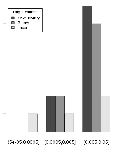
Figure 6: Number of significant P-values for each method

4 Conclusion

In this article, our main contribution has been to develop a co-clustering model taking into account a (mixture of) Gaussian co-variable. Applications have been made on simulated and real data sets. Our preliminary results are confirmed in previous studies in Africa. The method offers good classification performance on complex data sets (large number of variables and classes). This method can be useful in a wide variety of classification problems with Gaussian predictors and will allow us to discover new patterns of genes allowing to understand and evaluate the mechanism existing between genetics and malaria in an African population particularly in a Senegalese rural area. Further analysis could be done with more SNPs in another paper in preparation. Estimation is performed using a R package (with computational part in C++) that will be soon be available on the CRAN website https://cran.r-project.org/. Meanwhile the package is available on demand to the authors.

ieeetr

Appendix A Computing the (rows and columns) E-Step

For the E-Step $t_{ik}$ value maximize the fuzzy criterion given in equation (8). Derivative with respect to $t_{ik}$ gives

$$\frac{\partial\tilde{F}_{C}(\mathbf{t},\mathbf{r};\boldsymbol{\theta})}{\partial t_{ik}}=\log\pi_{k}+\sum_{j,\ell}r_{j\ell}\log f_{k\ell}(x_{ij},\mathbf{y}_{i};\boldsymbol{\theta})-\log t_{ik}-1.$$

Equating this equation to zero, taking exponential and recalling that $\sum_{k}t_{ik}=1$, we obtain that $t_{ik}$ is updated as

$$t_{ik}^{(c+1)}=\frac{\pi_{k}^{(c)}\prod_{j,l}\left[f(x_{ij},\mathbf{y}_{i};\boldsymbol{\theta}^{(c)})\right]^{r_{jl}^{(c)}}}{\sum_{k}\prod_{j,l}\left[f(x_{ij},\mathbf{y}_{i};\boldsymbol{\theta}^{(c)})\right]^{r_{jl}^{(c)}}}.$$

For numerical reason, we prefer to compute the logarithm of this expression which is

$$\log(t_{ik}^{(c+1)})\propto\log(\pi_{k}^{(c)})+\sum_{j,l}r_{jl}^{(c)}\log f(x_{ij},\mathbf{y}_{i};\boldsymbol{\theta}^{(c)}).$$

Recall that (see equation 3)

$$\log f(x_{ij}|\mathbf{y}_{i};\boldsymbol{\beta}_{kl}^{(c)}) = x_{ij}\log(\operatorname{logis}(\mathbf{y}_{i}^{T}\boldsymbol{\beta}_{kl}^{(c)}))+(1-x_{ij})\log(1-\operatorname{logis}(\mathbf{y}_{i}^{T}\boldsymbol{\beta}_{kl}^{(c)}))$$

$$= \log(1-\operatorname{logis}(\mathbf{y}_{i}^{T}\boldsymbol{\beta}_{kl}^{(c)}))+x_{ij}\log\left(\frac{\operatorname{logis}(\mathbf{y}_{i}^{T}\boldsymbol{\beta}_{kl}^{(c)})}{1-\operatorname{logis}(\mathbf{y}_{i}^{T}.\boldsymbol{\beta}_{kl})}\right)$$

$$= \log(1+\exp(\mathbf{y}_{i}^{T}\boldsymbol{\beta}_{kl}^{(c)}))+x_{ij}\mathbf{y}_{i}^{T}\boldsymbol{\beta}_{kl}^{(c)}$$

giving

$$\log t_{ik}^{(c+1)}\propto\log\pi_{k}^{(c)}+\sum_{j,l}r_{jl}^{(c)}x_{ij}\mathbf{y}_{i}^{T}.\boldsymbol{\beta}_{kl}^{(c)}-\sum_{l}r_{.l}^{(c)}\log(1+e^{\mathbf{y}_{i}^{T}.\boldsymbol{\beta}_{kl}^{(c)}})+m\;\log\phi(\mathbf{y}_{i};\boldsymbol{\mu}_{k}^{(c)},\boldsymbol{\Sigma}_{k}^{(c)}).$$

Similar computation gives for $r_{jl}$

$$\log(r_{jl}^{(c+1)})\propto\log\left(\rho_{l}^{(c)}\right)+\sum_{i,k}t_{ik}^{(c+1)}\left(x_{ij}\mathbf{y}_{i}^{T}\boldsymbol{\beta}_{kl}^{(c+1/2)}-\log\left(1+e^{\mathbf{y}_{i}^{T}.\boldsymbol{\beta}_{kl}^{(c+1/2)}}\right)\right).$$

Observe that the Gaussian distribution does not depend of $j$ nor $l$. This term become constant when summing over $i$ and $k$ and disappears when $r_{jl}$ values are normalized.

Appendix B Computing the M-Step

For the M-Step, we use a Newton-Raphson algorithm in order to solve the equation (10). For each pair $(k,l)$ the function to maximize can be written

$$\ell_{k,l}(\boldsymbol{\beta})=\sum_{i,j}\left(r_{jl}t_{ik}x_{ij}\mathbf{y}_{i}^{T}\boldsymbol{\beta}-r_{jl}t_{ik}\log({1+\exp(\mathbf{y}_{i}^{T}.\boldsymbol{\beta})})\right)$$

The first derivative with respect to the d-th coordinate $\beta_{d}$ is

$$\frac{\partial\ell_{k,l}(\beta)}{\partial\beta_{d}}=\sum_{i,j}\left(r_{jl}t_{ik}x_{ij}y_{i,d}-r_{jl}t_{ik}y_{i,d}\frac{\exp(\mathbf{y}_{i}^{T}\boldsymbol{\beta})}{1+\exp(\mathbf{y}_{i}^{T}\boldsymbol{\beta})}\right)$$

giving the following expression for the gradient

$$\nabla_{\beta}\ell_{k,l}(\boldsymbol{\beta})=Y^{T}D(X-\boldsymbol{\mu})$$

with $Y=\left[\mathbf{y}_{i}\right]_{i=1}^{N}$, $X=\left[\sum_{j}r_{jl}x_{ij}\right]_{i=1}^{N}$, $\boldsymbol{\mu}=\left[r_{.l}\frac{\exp(\mathbf{y}_{i}^{T}.\boldsymbol{\beta})}{1+\exp(\mathbf{y}_{i}^{T}\boldsymbol{\beta})}\right]_{i=1}^{N}$, $D=\mathop{\mathrm{diag}}(t_{ik})_{i=1}^{N}$ The second derivative with respect to $\beta_{d}$ and $\beta_{d^{{}^{\prime}}}$ is

$$\frac{\partial^{2}\ell_{k,l}(\boldsymbol{\beta})}{\partial\beta_{d}\partial\beta_{d^{{}^{\prime}}}}=-\sum_{i,j}\left(r_{jl}t_{ik}y_{i,d}y_{i,d^{{}^{\prime}}}\frac{\exp(\mathbf{y}_{i}^{T}\boldsymbol{\beta})}{(1+\exp(\mathbf{y}_{i}^{T}\boldsymbol{\beta}))^{2}}\right)$$

giving the following expression for the hessian

$$H_{\beta}=-Y^{t}DWY\qquad\mbox{ with }\qquad W=\mathop{\mathrm{diag}}\left(\frac{r_{.l}\,\exp(\mathbf{y}_{i}^{T}.\boldsymbol{\beta})}{(1+\exp(\mathbf{y}_{i}^{T}\boldsymbol{\beta}))^{2}}\right)=\mathop{\mathrm{diag}}\left(r_{.l}\,\mu_{i}(1-\mu_{i})\right)$$

References

- [1] S. C. Madeira and A. L. Oliveira, “Biclustering algorithms for biological data analysis: a survey,” IEEE/ACM Transactions on Computational Biology and Bioinformatics (TCBB), vol. 1, no. 1, pp. 24–45, 2004.
- [2] I. S. Dhillon, “Co-clustering documents and words using bipartite spectral graph partitioning,” in Proceedings of the seventh ACM SIGKDD international conference on Knowledge discovery and data mining, KDD ’01, (New York, NY, USA), pp. 269–274, ACM, 2001.
- [3] G. Xu, Y. Zong, P. Dolog, and Y. Zhang, “Co-clustering analysis of weblogs using bipartite spectral projection approach,” Knowledge-Based and Intelligent Information and Engineering Systems, pp. 398–407, 2010.
- [4] J. Guan, G. Qiu, and X.-Y. Xue, “Spectral images and features co-clustering with application to content-based image retrieval,” in Multimedia Signal Processing, 2005 IEEE 7th Workshop on, pp. 1–4, IEEE, 2005.
- [5] G. Govaert and M. Nadif, “Clustering with block mixture models,” Pattern Recognition, vol. 36, no. 2, pp. 463 – 473, 2003.
- [6] P. Bhatia, S. Iovleff, and G. Govaert, “blockcluster: An r package for model-based co-clustering,” Journal of Statistical Software, Articles, vol. 76, no. 9, pp. 1–24, 2017.
- [7] A. Dempster, N. Laird, and D. Rubin, “Maximum likelihood from incomplete data with the em algorithm (with discussion),” Journal of the Royal Statistical Society, Series B, vol. 39, p. 1, 1997.
- [8] R. Hathaway, “Another interpretation of the em algorithm for mixture distributions,” Statistics & Probability Letters, vol. 4, no. 2, pp. 53–56, 1986.
- [9] R. Neal and G. Hinton, “A view of the em algorithm that justifies incremental, sparse, and other variants,” NATO ASI SERIES D BEHAVIOURAL AND SOCIAL SCIENCES, vol. 89, pp. 355–370, 1998.
- [10] G. Schwarz et al., “Estimating the dimension of a model,” The annals of statistics, vol. 6, no. 2, pp. 461–464, 1978.
- [11] C. Keribin, V. Brault, G. Celeux, G. Govaert, et al., “Model selection for the binary latent block model,” in Proceedings of COMPSTAT, vol. 2012, 2012.
- [12] C. Keribin, V. Brault, G. Celeux, and G. Govaert, “Estimation and selection for the latent block model on categorical data,” Statistics and Computing, vol. 25, no. 6, pp. 1201–1216, 2015.
- [13] B. Maiga, A. Dolo, S. Campino, N. Sepulveda, P. Corran, K. A. Rockett, M. Troye-Blomberg, O. K. Doumbo, and T. G. Clark, “Glucose-6-phosphate dehydrogenase polymorphisms and susceptibility to mild malaria in dogon and fulani, mali,” Malaria journal, vol. 13, no. 1, p. 270, 2014.
- [14] A. Manjurano, N. Sepulveda, B. Nadjm, G. Mtove, H. Wangai, C. Maxwell, R. Olomi, H. Reyburn, E. M. Riley, C. J. Drakeley, et al., “African glucose-6-phosphate dehydrogenase alleles associated with protection from severe malaria in heterozygous females in tanzania,” PLoS genetics, vol. 11, no. 2, p. e1004960, 2015.
- [15] O. Toure, S. Konate, S. Sissoko, A. Niangaly, A. Barry, A. H. Sall, E. Diarra, B. Poudiougou, N. Sepulveda, S. Campino, et al., “Candidate polymorphisms and severe malaria in a malian population,” PLoS One, vol. 7, no. 9, p. e43987, 2012.
- [16] T. N. Williams, “How do hemoglobins s and c result in malaria protection?,” The Journal of Infectious Diseases, vol. 204, no. 11, pp. 1651–1653, 2011.
- [17] E. Beet et al., “Sickle cell disease in the balovale district of northern rhodesia.,” East African medical journal, vol. 23, no. 3, pp. 75–86, 1946.
- [18] A. C. Allison, “Protection afforded by sickle-cell trait against subtertian malarial infection,” British medical journal, vol. 1, no. 4857, p. 290, 1954.
- [19] A. C. Allison, “The distribution of the sickle-cell trait in east africa and elsewhere, and its apparent relationship to the incidence of subtertian malaria,” Transactions of the Royal Society of Tropical Medicine and Hygiene, vol. 48, no. 4, pp. 312–318, 1954.