Data-Driven Inference, Reconstruction, and Observational Completeness of Quantum Devices

Abstract

The range of a quantum measurement is the set of outcome probability distributions that can be produced by varying the input state. We introduce data-driven inference as a protocol that, given a set of experimental data as a collection of outcome distributions, infers the quantum measurement which is, i) consistent with the data, in the sense that its range contains all the distributions observed, and, ii) maximally noncommittal, in the sense that its range is of minimum volume in the space of outcome distributions. We show that data-driven inference is able to return a unique measurement for any data set if and only if the inference adopts a (hyper)-spherical state space (for example, the classical or the quantum bit).

In analogy to informational completeness for quantum tomography, we define observational completeness as the property of any set of states that, when fed into any given measurement, produces a set of outcome distributions allowing for the correct reconstruction of the measurement via data-driven inference. We show that observational completeness is strictly stronger than informational completeness, in the sense that not all informationally complete sets are also observationally complete. Moreover, we show that for systems with a (hyper)-spherical state space, the only observationally complete simplex is the regular one, namely, the symmetric informationally complete set.

I Introduction

In quantum theory, as a consequence of the Born rule, a measurement can always be seen as a linear mapping from the set of states (i.e., density operators) into the set of probability distributions over the measurement outcomes. In fact, some axiomatic approaches identify quantum measurements with the set of such mappings: in such a case, the resulting distribution, i.e., the image of the state of the system undergoing the measurement, receives the natural operational interpretation of distribution over the measurement outcomes [1].

When thinking of measurements as linear mappings, the image of the set of all states under a given measurement—also known as the measurement’s range—turns out to be a very important mathematical object in quantum measurement theory. For example, given two quantum measurements, the range of one includes the range of the other, if and only if the former can simulate the latter by means of a suitable statistical transformation [2, 3, 4], independently of the state being measured. Quantum measurements, hence, can be compared by comparing the corresponding ranges, thus establishing a deep connection between quantum measurement theory and the theory of majorization and statistical comparison [5, 6], with ramified consequences in both theory and applications [7, 8, 9, 10, 11, 12, 13, 14, 15, 16].

In this paper we exploit the correspondence between measurements and their ranges to propose a method to derive an inference about an unknown quantum measurement, based solely on the outcome distributions observed, without any knowledge about the exact states that gave rise to such distributions. As we observe in what follows, such a method can be naturally divided into two parts. In the first part, one defines an inference rule, which formulates in an abstract way the rules that we choose to use when reasoning in the presence of incomplete information. For the problem at hand, such rules accept as input a set of outcome distributions and return as output a set of quantum measurements. For this reason, we name our inference rule “data-driven inference (DDI) of quantum measurements.” The measurements inferred via DDI are consistent with the input data and are maximally noncommittal, in the sense that their ranges contain the input data and are of minimum volume in the space of outcome distributions. DDI need not aim to infer the “true” quantum measurement, as there need not be any such “entity” at this stage. As an application, we implement an algorithm for the machine learning of qubit measurements based on data-driven inference, and we test it on data generated by the IBM Q Experience quantum computer.

In the second part, one needs to show that it is indeed possible to construct a real experiment so that DDI leads to the correct assignment for the unknown measurement. The goal here is reminiscent of that of conventional quantum measurement tomography ([17, 18, 19, 20, 21, 22, 23]), namely, the reconstruction of an unknown measurement from the statistics collected in a sequence of experimental trials. However, while the data analysis performed in measurement tomography requires the knowledge of the states that were fed into the unknown measurement, DDI reconstruction only requires the analysis of the bare outcome distributions: the state-preparator could, for example, emit a different unknown state at each repetition of the experiment, and DDI reconstruction would still be applicable.

In what follows, we expound the theory of data-driven inference and reconstruction for finite dimensional systems. As this is based on the correspondence between measurements and their ranges, three main problems arise and are addressed.

The first problem is to seek for a general method to infer a range given a set of outcome distributions. As a possible solution, in what follows, we propose that the measurement range to be inferred, in the face of a set of experimental data, should be the smallest one containing all the observed data. Recalling that the range of a measurement is directly related with the ability to simulate other measurements [2], our principle is equivalent to say that the measurements to be inferred should be the weakest possible, compatibly with the data. Our inference rule hence encapsulates a principle of “self-consistent minimality” that we believe constitutes a natural way to reason in the presence of incomplete information. We show that the only systems for which DDI always leads to a unique range for any set of data, among all generalized probabilistic theories [24, 25, 26, 27, 28, 29, 30], are those with (hyper)-spherical state space, such as the classical and the quantum bit. This can be interpreted as an “epistemic reconstruction” of such systems, regarded as epistemic hypotheses onto which to base our reasoning, rather than actual entities to be operationally characterized [31, 32, 33, 34].

The second problem consists of understanding to which extent the correspondence between a measurement and its range can be inverted, that is, to what extent a measurement can be characterized if only its range is given. In this respect, in what follows, we show that the correspondence measurement-range is invertible, but only up to the action of a symmetry transformation leaving the state space of the system invariant. This is something to be expected when directly working in the space of outcome distributions, and we consider this to be a feature, rather than a limitation, of DDI.

The third problem is to understand how an experimentalist, in complete control of their laboratory, can produce experimental data, which are rich enough to reconstruct, via DDI, the “correct” range of a measurement. That is, we want to understand whether, in order to recover the correct range by DDI, an infinite set of states needs to be prepared and sent through the measurement apparatus, or whether a finite set of states, and possibly the same ones for any measurements, suffice (we remark that, in contrast to the data analysis of quantum measurement tomography, DDI does not require the knowledge of such states). This problem is analogous to the problem in quantum tomography to construct a standard apparatus that work whatever it is to be reconstructed. As the problem in quantum tomography is solved by informationally complete apparatus, the analogous problem in DDI reconstruction is solved by what we call observationally complete (OC) apparatus. More precisely, OC sets of states are sets whose image contains the same statistical information as the entire range. Of course, since DDI does not rely on the knowledge of the states, it is not possible for DDI to certify whether the states fed into the measurement were OC.

We show that the property of observational completeness is strictly stronger than informational completeness, thus constituting a new “Bureau of Standards” in terms of DDI reconstruction. To this aim we show that, for systems with (hyper)-spherical state space such as the classical and quantum bits, the only observationally complete simplex is the regular simplex, that is, the symmetric informationally complete (SIC) one [35, 36, 37, 38, 39, 40]. Data-driven inference and reconstruction, hence, naturally lead to the notion of SIC apparatus by looking only at the set of outcome distributions, thus providing a completely new viewpoint on the discussion about SIC apparatus and their “natural occurrence” in quantum theory.

The structure of the paper follows the above discussion. In the first section, we introduce data-driven inference as the inference of the minimal range consistent with the observed distributions, and we show that the inferred range is unique for any set of outcome distributions only for systems with (hyper)-spherical state space. We also prove that the range of a measurement identifies such a measurement up to gauge symmetries. In the second section, we introduce the property of observational completeness and show that it represents a strictly stronger condition than informational completeness. For systems with (hyper)-spherical state space, we show that the minimal observationally complete set of states happens to be SIC. In the third section, we implement a protocol for the machine learning of qubit measurements based on data-driven inference and reconstruction, and we test it on data generated by the IBM Q Experience quantum computer.

II Data-driven inference

Let us consider an experimental setup involving two boxes equipped with $m$ buttons and $n$ light bulbs, respectively. This situation is depicted in Fig. 1.

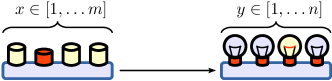
Figure 1: The experimental setup consists of two uncharacterized boxes equipped with $m$ buttons and $n$ light bulbs, respectively. At each run, Alice presses button $x$ and observes outcome $y$, thus recording vectors $\{\mathbf{p}_{x}\in\mathbb{R}^{n}\}$, whose $y$-th entry is the frequency of outcome $y$ given input $x$.

At each run of the experiment, a theoretician, say Alice, presses button $x$ and observes outcome $y$. She records the vectors $\{\mathbf{p}_{x}\in\mathbb{R}^{n}\}$, whose $y$-th entry is the frequency of outcome $y$ given input $x$.

We address the problem of inferring all the measurements $\hat{M}$ that are self-consistent and minimal for observed frequencies $\{\mathbf{p}_{x}\}$, in an i.i.d. hypothesis for $\hat{M}$. To formalize this idea, notice that any $n$-outcome measurement $M$ induces a linear transformation from the state space $\mathbb{S}$ (the set of all states available to the system) to the space of outcome distributions $\mathbb{R}^{n}$. The range of such a transformation, denoted by $M(\mathbb{S})$, represents the distributions compatible with measurement $M$. Hence, given some prior information about a state space $\mathbb{S}$, the inferred linear transformations $\hat{M}$ minimize the volume of their ranges $\hat{M}(\mathbb{S})$ under the self-consistency constraints $\hat{M}(\mathbb{S})\supseteq\{\mathbf{p}_{x}\}$. This naturally identifies two steps in the inference of $\hat{M}$: i) the inference of the (possibly not unique) minimum-volume range $\hat{\mathcal{R}}$ such that $\hat{\mathcal{R}}\supseteq\{\mathbf{p}_{x}\}$, and ii) the characterization of all the linear transformations $\hat{M}$ with given range $M(\mathbb{S})=\hat{\mathcal{R}}$.

Let us start addressing the first step, that is, the inference of the (possibly not unique) minimum-volume range $\hat{\mathcal{R}}$ such that $\hat{\mathcal{R}}\supseteq\{\mathbf{p}_{x}\}$. Since such an inference is solely driven by the data, we call it data-driven inference (see also [41, 42]):

Definition 1 (Data-driven inference).

For any set $\{\mathbf{p}_{x}\}$, we denote by $\operatorname{\mathtt{ddi}}(\{\mathbf{p}_{x}\}|\mathbb{S})$ the data-driven inference map

$$\operatorname{\mathtt{ddi}}\left(\{\mathbf{p}_{x}\}\big{|}\mathbb{S}\right)=\operatorname*{argmin}_{\mathcal{R}\supseteq\left\{\mathbf{p}_{x}\right\}}\operatorname{\mathcal{V}}\left(\mathcal{R}\right),$$ (1)

where $\operatorname{\mathcal{V}}(\mathcal{R})$ denotes the Euclidean volume of $\mathcal{R}$ and the minimization is over subsets $\mathcal{R}\subseteq\mathbb{R}^{n}$ corresponding to linear transformations of the state space $\mathbb{S}$ that lie on the affine subspace generated by $\{\mathbf{p}_{x}\}$.

If the prior information does not specify a single state space $\mathbb{S}$, the minimum in Eq. (1) is meant to run also over all such sets.

An intuitive geometrical interpretation for Definition 1 is illustrated by the following two examples.

First, let $\mathbb{S}$ be a (hyper)-sphere $\Sigma$. This scenario encompasses the cases of classical and quantum bits, where the set $\mathbb{S}$ is a one-dimensional and a three-dimensional sphere, respectively. In this case, the optimization in Eq. (1) is over affine transformations of a sphere, that is, ellipsoids. It follows [43, 44] that the range returned by map $\operatorname{\mathtt{ddi}}$ is unique for any input set $\{\mathbf{p}_{x}\}$, and one has that

$$\operatorname{\mathtt{ddi}}\left(\left\{\mathbf{p}_{x}\right\}\;\big{|}\;\Sigma\right)=\left\{\operatorname{\mathtt{MVEE}}\left(\left\{\mathbf{p}_{x}\right\}\right)\right\},$$ (2)

where $\operatorname{\mathtt{MVEE}}$ denotes the minimum volume-enclosing ellipsoid, which is known to be a convex problem, and for which efficient computing algorithms are available [45]. This situation is illustrated in Fig. 2, left-hand side.

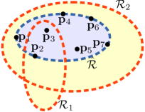
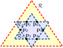
Figure 2: The figure provides a schematic representation of the space of distributions when $n=3$ (three outcomes, and hence the probability simplex is two-dimensional). Left: when the state space $\mathbb{S}$ is a sphere, the data-driven inference defined by Eq. (1) returns the minimum volume-enclosing ellipsoid $\hat{\mathcal{R}}$, which always exists unique, for the given set $\{\mathbf{p}_{x}\}$. Range $\mathcal{R}_{1}$ is not consistent with $\{\mathbf{p}_{x}\}$, while $\mathcal{R}_{2}$, although consistent, is not minimum volume. Right: when the state space $\mathbb{S}$ is a simplex, the data-driven inference defined by Eq. (1) returns the set of minimum volume-enclosing simplices (as these are generally not unique) $\hat{\mathcal{R}}_{1}$ and $\hat{\mathcal{R}}_{2}$ for the given set $\{\mathbf{p}_{x}\}$. Range $\mathcal{R}$ is not minimum volume.

Let us consider now, as a second example, the case in which the state space $\mathbb{S}$ is a regular simplex $\Delta$, as it is the case for classical systems. In this case, the optimization in Eq. (1) is over affine transformations of the simplex $\Delta$, which turn out to be simplices themselves. It is not difficult to find configurations of the set $\{\mathbf{p}_{x}\}$ of observed distributions, such that the range returned by the map $\operatorname{\mathtt{ddi}}$ is not unique. This situation is illustrated in Fig. 2, right-hand side.

In light of the previous examples, it is a natural question to ask for which state spaces $\mathbb{S}$ the range returned by the data-driven inference $\operatorname{\mathtt{ddi}}$ is always unique. The following Theorem, proved in the appendix, answers such a question.

Theorem 1.

The range returned by the data-driven inference $\operatorname{\mathtt{ddi}}(\{\mathbf{p}_{x}\}|\mathbb{S})$ is unique for any $\{\mathbf{p}_{x}\}$, if and only if the state space $\mathbb{S}$ is a (hyper)-sphere.

This result can be lifted to the level of a principle, singling out spherical state spaces $\mathbb{S}$, such as those of the classical and quantum bits, as those for which the map $\operatorname{\mathtt{ddi}}$ always returns a unique range. This principle rules out theories with more exotic elementary systems, such as PR-boxes[25] for which inference is not always unique. In this case, we speak of an epistemic principle, that is, a constraint on the state space seen as the hypothesis used by the observer as the base of their inference.

Let us now move on to the second step mentioned above, that is, the characterization of all the linear transformations $M$ with range $M(\mathbb{S})$ equal to a given inferred one $\hat{\mathcal{R}}$. Notice first that any transformation $U$ that leaves the state space $\mathbb{S}$ invariant, that is such that $U(\mathbb{S})=\mathbb{S}$, does not affect the range $M(\mathbb{S})$, that is $M(U(\mathbb{S}))=M(\mathbb{S})$. We refer to any such a transformation as a gauge symmetry. The following Theorem shows that accuracy up to gauge symmetries is indeed the optimal accuracy in the characterization of any informationally complete (i.e., invertible) $M$, given its range. (For non-informationally complete $M$, the statement, although conceptually similar, becomes technically more involved, so we postpone the general statement and its proof to the appendix.)

Theorem 2.

For any given state space $\mathbb{S}$, the range $M(\mathbb{S})$ of any informationally complete $M$ identifies $M$ up to gauge symmetries.

Although Theorem 2 is valid for any state space $\mathbb{S}$, for the sake of concreteness let us revisit our running example where $\mathbb{S}$ is a (hyper)-sphere $\Sigma$, in particular a qubit.

In the qubit case, the gauge symmetries correspond to unitary and anti-unitary transformations in the Hilbert space, hence, the range $M(\mathbb{S})$ identifies linear transformation $M$ up to unitary and anti-unitary transformations. However, Theorem 2 only guarantees the existence of such an identification, without providing an explicit construction. Reference [41] fills this gap by explicitly deriving all the linear transformations that correspond to any given (hyper)-ellipsoidal range. Such a result is provided a new simpler proof in appendix.

An algorithmic representation of data-driven inference is given in Fig. 3.

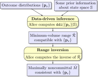
Figure 3: Algorithmic representation of data-driven inference.

III Data-driven reconstruction

In the previous section we introduced a principle of self-consistent minimality to guide the inference of a measurement given a set of observed outcome distributions. In this section, we consider the case in which the boxes with buttons and lights in Fig. 1 describe a physical state-preparator $\mathcal{S}$ and a physical measurement $M$, respectively. This situation is illustrated in Fig. 4.

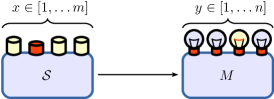
Figure 4: The same experimental setup as in Fig. 1, although this time the state preparator $\mathcal{S}$ is built by Bob, with the aim of enabling Alice to correctly infer measurement range $M(\mathbb{S})$, that is, for the inferred range $\hat{\mathcal{R}}$, one has $\hat{\mathcal{R}}=M(\mathbb{S})$.

The state-preparator $\mathcal{S}$ is built by an experimentalist, say Bob, with the aim of enabling Alice to correctly infer the measurement range $M(\mathbb{S})$ through DDI, that is, the inferred range $\hat{\mathcal{R}}$ satisfying $\hat{\mathcal{R}}=M(\mathbb{S})$, in the limit in which Alice presses each button infinitely many times. This task shares similarities with conventional measurement tomography, with the major difference that, in the latter, full knowledge of the state-preparator $\mathcal{S}$ is pivotal for Alice’s data analysis, whereas DDI solely depends on the observed outcome distributions and the knowledge of the state space $\mathbb{S}$.

Since it is sufficient to show that Bob is able to construct one such a state-preparator, we can assume, without loss of generality, that each button of the state preparator emits always the same state at each press, and that different buttons are associated with different states. Hence, the state-preparator $\mathcal{S}$ can be mathematically described as a set of states.

The probabilities $\{\mathbf{p}_{x}\}$ Alice observes are the image of the states in $\mathcal{S}$, that is, $\{\mathbf{p}_{x}\}=M(\mathcal{S})$. Correct inference imposes then that $M(\mathcal{S})$ contains all the statistical information that is available in the measurement range $M(\mathbb{S})$, and that such information can be extracted by data-driven inference. We call observationally complete (OC) any state preparator that allows for the correct inference of measurement $M$.

Definition 2 (Observational completeness).

A set of states $\mathcal{S}$ is said to be observationally complete for measurement $M$ whenever

$$\operatorname{\mathtt{ddi}}\left(M(\mathcal{S})\big{|}\mathbb{S}\right)=\left\{M(\mathbb{S})\right\}\;.$$ (3)

If the set is not OC, the set of inferred measurements may not contain the correct measurement, but measurements with ranges smaller than the correct measurement, or even measurements inequivalent (modulo gauge symmetries) to it.

Notice that observational completeness (OC-ness) plays an analogous role for data-driven reconstruction as informational completeness (IC-ness) plays for conventional measurement tomography. However, IC sets of states allow for the correct tomographic reconstruction of any measurement, while OC sets of states apparently depend on the measurement to be inferred.

Is this really the case? It turns out that, as long as the measurement is IC, by bypassing the linear transformation $M$ in Eq. (3) one obtains a condition equivalent to Eq. (3), as stated in the following theorem:

Theorem 3.

A set $\mathcal{S}$ of states is OC complete for any IC measurement, if and only if

$$\operatorname{\mathtt{ddi}}\left(\mathcal{S}\big{|}\mathbb{S}\right)=\left\{\mathbb{S}\right\}.$$ (4)

Notice that in Eq. (4) the map $\operatorname{\mathtt{ddi}}$ is applied to a set of states, as opposed to a set of probability distributions as it was the case so far.

Hence, any set $\mathcal{S}$ of states that is OC for some IC measurement, is also OC for any other IC measurement. Moreover, Eq. (4) provides a characterization of any such a set $\mathcal{S}$ in closed-form, namely, in a form which only depends on $\mathcal{S}$ alone, in contrast with Definition 2 that also depends on $M$. Such a characterization can be used to readily check if any given set $\mathcal{S}$ is OC for any IC measurement.

More generally, even if $M$ is not an IC measurement, one can write a condition equivalent to Eq. (3) (and conceptually analogous to Eq. (4), just technically more involved) that depends on $M$ only through its support. Hence, any set $\mathcal{S}$ of states that is OC for $M$ is also OC for any other measurement with the same support. In other words, it is universally OC on such a support. A fully general version of Theorem 3 is provided in the appendix.

Notice that, while OC sets of states are universal within a given subspace, IC sets of states are universal for any subspace and all of its subspaces. In fact, it is easy to see that the only set of states that is OC for any measurement $M$ is trivially the state space $\mathbb{S}$.

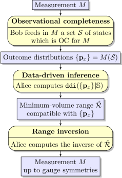
Figure 5: Algorithmic representation of data-driven reconstruction.

Although Theorem 3 is valid for any state space $\mathbb{S}$, for the sake of concreteness let us revisit our running example where $\mathbb{S}$ is a (hyper)-sphere.

In light of Eq. (2), Theorem 3 states that a set $\mathcal{S}$ of states is OC for IC measurements if and only if its minimum volume-enclosing ellipsoid coincides with the (hyper)-sphere $\Sigma$, that is

$$\operatorname{\mathtt{MVEE}}(\mathcal{S})=\Sigma.$$ (5)

In the appendix, as a consequence of Ref. [46], we show that such a condition is satisfied when $\mathcal{S}$ is a regular simplex. This situation is illustrated in Figure 6, left-hand side. Moreover, we show that, as a consequence of Ref. [47], also the converse is true, namely, that such a condition is violated whenever $\mathcal{S}$ is an irregular simplex (see Figure 6, right-hand side). Hence, for simplices, OC-ness is equivalent to symmetric IC-ness and, therefore, the SIC set of states is the minimal (in terms of cardinality) OC set. This provides an operational interpretation of symmetric informational completeness in terms of data-driven inference and reconstruction. It is tempting to conjecture that this equivalence holds for any quantum system, not just the qubit.

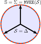
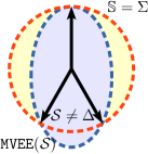
Figure 6: The figure provides a two-dimensional representation of the spherical state space $\mathbb{S}$ (orange line) and of the minimum volume-enclosing ellipsoid (blue line) for the simplicial set $\mathcal{S}$ of states (black vectors). Left: when $\mathcal{S}$ coincides with the regular simplex $\Delta$, its minimum-volume enclosing ellipsoid coincides with the sphere $\Sigma$, hence, due to Theorem 3, $\mathcal{S}$ is observationally complete. Right: when $\mathcal{S}$ does not coincide with the regular simplex $\Delta$, its minimum volume-enclosing ellipsoid does not coincide with the sphere $\Sigma$, hence, due to Theorem 3, $\mathcal{S}$ is not observationally complete.

Although it is easy to see that any set of states which is OC on a subspace, is also IC on that subspace, the previous example shows that the vice-versa is not true. Indeed, any simplex, whether regular or not, is trivially IC on its support. Hence, OC-ness is a strictly stronger condition than IC-ness. In this sense, OC-ness defines a new “Bureau of Standards” in terms of data-driven inference and reconstruction.

IV Machine larning of qubit measurements

In this Section, we first provide an algorithm for the data-driven inference of measurements of any system with (hyper)-spherical state space, and then we apply it to the data-driven reconstruction of a qubit measurement implemented with the IBM quantum computer.

Let us begin by discussing the algorithm for the data-driven inference. As shown by Eq. (2), for (hyper)-spherical state space $\mathbb{S}=\Sigma$ the data-driven inference algorithm $\operatorname{\mathtt{ddi}}$ can be written in terms of a minimum volume enclosing ellipsoind algorithm $\operatorname{\mathtt{MVEE}}$. Efficient algorithms for the computation of $\operatorname{\mathtt{MVEE}}$ (quadratic in the dimension and linear in the number of points) can readily be found [45, 48], but in general assume that the affine space generated by the input set coincides with the full linear space. Hence, given a set $\{\mathbf{p}_{x}\}$, to compute $\operatorname{\mathtt{ddi}}(\{\mathbf{p}_{x}\}|\Sigma)$ one proceeds as follows:

1. Find an isometry $V$ such that $V^{T}V=\openone$ and $VV^{T}$ is the projector on the linear subspace homogeneous to the affine subspace generated by $\{\mathbf{p}_{x}\}$.

2. Compute $\operatorname{\mathtt{MVEE}}(V^{T}\{\mathbf{p}_{x}-\mathbf{p}_{0}\})$, where by construction the affine subspace generated by $V^{T}\{\mathbf{p}_{x}-\mathbf{p}_{0}\}$ is now full dimensional, thus obtaining an ellipsoid in the form $(\tilde{\mathbf{p}}-\tilde{\mathbf{t}})^{T}\tilde{Q}^{-1}(\tilde{\mathbf{p}}-\tilde{\mathbf{t}})\leq 1$.

3. The output of $\operatorname{\mathtt{ddi}}(\{\mathbf{p}_{x}\}|\Sigma)$ is the singleton given by the ellipsoid

   $$\begin{cases}\left(\openone-QQ^{+}\right)\left(\mathbf{p}-\mathbf{t}\right)=0,\\ \left(\mathbf{p}-\mathbf{t}\right)^{T}Q^{+}\left(\mathbf{p}-\mathbf{t}\right)\leq 1,\end{cases}$$

   where $Q\mathrel{\mathop{\ordinarycolon}}=V\tilde{Q}V^{T}$ and $\mathbf{t}\mathrel{\mathop{\ordinarycolon}}=V\tilde{\mathbf{t}}+\mathbf{p}_{0}$.

We tested our algorithm on the set $\{\mathbf{p}_{0},\mathbf{p}_{1},\mathbf{p}_{2}\}$ as follows (later on we show how this data was obtained):

$$\mathbf{p}_{0}\simeq\begin{bmatrix}0.48\\ 0.05\\ 0.24\\ 0.23\end{bmatrix},\quad\mathbf{p}_{1}\simeq\begin{bmatrix}0.21\\ 0.32\\ 0.42\\ 0.05\end{bmatrix},\quad\mathbf{p}_{1}\simeq\begin{bmatrix}0.17\\ 0.33\\ 0.11\\ 0.39\end{bmatrix}$$ (6)

The minimum-volume enclosing ellipsoid for the set $\{V^{T}(\mathbf{p}_{x}-\mathbf{p}_{0})\}$, as given in the second step of our algorithm, is depicted in Fig. 7.

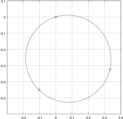
Figure 7: The figure depicts the three points $V^{T}(\mathbf{p}_{x}-\mathbf{p}_{0})$ (circles) for $x=0,1,2$, where $\bf{p}_{x}$’s are given by Eq. (6), and their minimum-volume enclosing ellipsoid, according to the second step of our algorithm for the data-driven inference of qubit measurements.

The correlation matrix $Q$ and the vector $t$, as reconstructed by the third step of our algorithm, are given by

$$Q\simeq 10^{-2}\begin{bmatrix}3.8&-3.6&0&-0.1\\ -3.6&3.4&0.2&0\\ 0&0.2&3.3&-3.4\\ -0.1&0&-3.4&3.6\end{bmatrix},\quad\mathbf{t}\simeq\begin{bmatrix}0.29\\ 0.23\\ 0.26\\ 0.22\end{bmatrix}.$$ (7)

As a consequence of Theorem 2, through range inversion this allows for the data-driven inference of the POVM up to gauge symmetries, that is, an overall unitary or anti-unitary transformation. In particular, as shown in Ref. [41] (an alternative, more compact proof is given in the appendix), any measurement $\{\pi_{y}\}$ compatible with correlation matrix $Q$ and vector $t$ can be obtained by inverting the following system:

$$\begin{cases}Q_{x,y}=\frac{1}{2}\operatorname{Tr}[\pi_{x}\pi_{y}]-\frac{1}{4}\operatorname{Tr}[\pi_{x}]\operatorname{Tr}[\pi_{y}],\\ t_{x}=\frac{1}{2}\operatorname{Tr}[\pi_{x}].\end{cases}$$

Let us now discuss the data-driven reconstruction, that is, the way in which the data in Eq. (6) was generated. Such data was generated by the IBM Q Experience quantum computer. The ideal circuit consists of the preparation of a trine set $\{\phi_{x}\}$ of states, which, as observed in Fig. 6 is observationally complete for any real measurement, and the measurement of two mutually unbiased basis, as depicted in Fig. 8.

X

X

Figure 8: The orange gate (top left) represents the preparation of the trine ensemble (from top to bottom, states $\phi_{0}$, $\phi_{1}$ and $\phi_{2}$). All other gates represent a Naimark extension of a measurement consisting of two mutually unbiased basis.

This allows one to compare the correlation matrix $Q$ and the vector $\mathbf{t}$ given in Eq. (7) (from which one can recover the inferred measurement up to gauge symmetries through range inversion) with the ideal ones, given by:

$$Q=\frac{1}{16}\begin{pmatrix}1&-1&0&0\\ -1&1&0&0\\ 0&0&1&-1\\ 0&0&-1&1\end{pmatrix},\quad\mathbf{t}=\frac{1}{4}\begin{pmatrix}1\\ 1\\ 1\\ 1\end{pmatrix}.$$

An analysis of the noise affecting the IBM backend is however out of the scope of this manuscript.

V Conclusion

In this work we introduced data-driven inference as a rule to output the maximally noncommittal measurement consistent with a set of observed distributions. We showed that the inference is possible in principle up to gauge symmetries, that is, symmetries of the state space of the system at hand, and that this accuracy limit is achieved for (hyper)-spherical state spaces. Then, we considered the task of reconstructing an unknown measurement via DDI. To this aim, we introduced observationally complete sets of states, as those enabling a correct inference universally, that is, for any unknown measurement on a given support. Deriving a closed-form characterization of observational completeness allowed us to show that, while observational completeness is a strictly stronger condition than informational completeness, in the case of (hyper)-spherical state space OC-ness with minimum number of states is equivalent to SIC-ness. In this way, the protocol of data-driven inference provides SIC sets with a novel, entirely operational interpretation.

Appendix

While, for the sake of clarity, in the previous sections we focused on the data-driven inference of measurements, in these appendices we extend the formalism to encompass the case of data-driven inference of families of states, thus justifying the word “devices” in our title. Finally, rather than restricting the presentation to the quantum case, here we consider general probabilistic theories.

Appendix A General framework

A physical system can be defined by giving a set of states and a set of effects, representing respectively the preparations and the observations of the system. An effect $a\in\mathbb{E}$ is a linear map that takes a state $\rho$ as an input and outcomes a probability $p(a|\rho)\mathrel{\mathop{\ordinarycolon}}=a(\rho)$. Since randomization of different experimental setups is in itself another valid experiment, it is natural to endow the set of states and the set of effects with a linear structure and allow for any convex combination of states and effects. By linear extension, it is also natural to introduce the real vector spaces generated by any real linear combinations of states and effects. Restricting to the finite dimensional case, the linear space of states and the linear space of effects are dual to each other and both isomorphic to $\mathbb{R}^{\ell}$ for some natural number $\ell$ which is called the linear dimension of the system.

We assume that the physical theory is causal. A probabilistic theory is causal if there exists a unique deterministic effect $e\in\mathbb{E}$, and deterministic states are those states such that $e(\rho)=1$. Therefore, states can always be normalized as $\overline{\rho}\mathrel{\mathop{\ordinarycolon}}=\rho/e(\rho)$ and every state is proportional to a deterministic one. For this reason, the full set of states of any causal theory is completely specified by the set of deterministic states. We denote by $\mathbb{S}$ the set of normalized (or deterministic) states of the theory and by $\mathbb{E}$ the set of effects of the theory.

By choosing an arbitrary basis, we can give a geometric representation of $\mathbb{S}$ and $\mathbb{E}$ as subset of $\mathbb{R}^{\ell}$: $\mathbb{S}$ will be a convex set contained in a strictly affine $(\ell-1)$-dimensional subspace, while $\mathbb{E}$ will be a “bicon-ish” shaped solid (see Fig. 9).

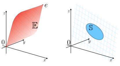
Figure 9: Vectorial representation of the a system $(\mathbb{S},\mathbb{E})$ of linear dimension $\ell=3$. Both the set of normalized states $\mathbb{S}$ and the set of effects $\mathbb{E}$ can by represented as convex subsets of the vector space $\mathbb{R}^{3}$. Left: The convex set of effects $\mathbb{E}$ corresponds to a truncated cone. The truncated cone contains the two points $(0,0,0)$ and $(1,1,1)$, which correspond to the null effect and to the deterministic effect $e$ respectively. Right: The convex set of normalized states $\mathbb{S}$. This set contains all states $\rho$ such that $e(\rho)=1$, and is then merged in an affine space with dimension $\ell-1$ (in this case a two-dimensional space).

Measurements are a family of effects $\{a_{y}\}_{y=1}^{n}$ such that $\sum_{y=1}^{n}a_{y}=e$, $\forall\rho\in\mathbb{S}$. Since any state can be regarded as a vector in $\mathbb{R}^{\ell}$, any measurement induces a linear map $M\in\mathfrak{M}_{{n}\times{\ell}}$ defined as follows

$$M\mathrel{\mathop{\ordinarycolon}} \,\mathbb{R}^{l}\rightarrow\mathbb{R}^{n}$$

$$\rho_{x}\mapsto\mathbf{p}_{x},\qquad p_{x}^{y}\mathrel{\mathop{\ordinarycolon}}=a_{y}(\rho_{x}).$$

(each row of $M\in\mathfrak{M}_{{n}\times{\ell}}$ corresponds to an effect). Any state is mapped into a point in $\mathbb{R}^{n}$ (see the Top Fig. 10). Analogously, since any effect $a_{x}$ corresponds to a vector in $\mathbb{R}^{\ell}$, any family of states $\{\rho_{y}\}_{y=1}^{n}$ induces a linear map defined as follows

$$R\mathrel{\mathop{\ordinarycolon}}\, \mathbb{R}^{l}\to\mathbb{R}^{n}$$

$$a_{x}\mapsto\mathbf{p}_{x},\qquad{p}^{y}_{x}\mathrel{\mathop{\ordinarycolon}}=\rho_{y}(a_{x}).$$

(each row of $R\in\mathfrak{M}_{{n}\times{\ell}}$ corresponds to a state). Any effect is mapped in a point in $\mathbb{R}^{n}$ (see the Bottom Fig. 10).

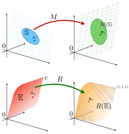
Figure 10: Top: The linear map $M$ corresponding to a measurement. Bottom: The linear map $R$ corresponding to a family of states.

For example, in quantum theory, any system is associated with a $d$-dimensional Hilbert space $\mathcal{H}$, states and effects are represented by positive semi-definite operators on $\mathcal{H}$, and conditional probabilities are given by the Born rule: $a_{y}(\rho_{x})\mathrel{\mathop{\ordinarycolon}}=\operatorname{Tr}[a_{y}\rho_{x}]$. States and effects are represented by vectors in the real space $\mathbb{R}^{\ell}$ with $\ell=d^{2}$. As an example, any qubit ($d=2$) normalized state $\rho=\tfrac{1}{2}\sum_{i=0}^{3}r^{i}\sigma_{i}$ is univocally associated to a vector $(r^{0},r^{1},r^{2},r^{3})^{T}\in\mathbb{R}^{4}$. Here, the condition $r^{0}=1$ guarantees that $\operatorname{Tr}[\rho]=1$, while the condition $|r|\leq 1$ for Bloch vector $\mathbf{r}\mathrel{\mathop{\ordinarycolon}}=(r^{1},r^{2},r^{3})^{T}$, where $\{\sigma_{i}\}_{i=1}^{3}$ are the Pauli matrices, guarantees that $\rho\geq 0$. The set of normalized states, identified by the constraint $r^{0}=1$, is geometrically represented by a sphere (the Bloch sphere) contained in a $3$-dimensional strictly affine subspace of $\mathbb{R}^{4}$.

As a second example, in classical theory the set of normalized states of any system with linear dimension $\ell$ is an $\ell$-simplex, e.g. a segment for the bit system $\ell=1$ and a triangle for the trit system $\ell=2$.

In the literature, toy models have been proposed whose convex set of states (and effects) differs from both the quantum and the classical ones. The most notable example are the PR-boxes, whose convex set of states of linear dimension $\ell=3$ is a square.

Appendix B Data-driven inference

The data-driven inference (DDI) of quantum measurements, presented in the Main Text, is a protocol that allows to infer a preferred (according to a maximally noncommittal criterion) measurement from a set of data interpreted as the outcome distributions of an experiment. The maximally noncommittal criterion is very natural: among the set of measurements whose range includes the experimental points, we choose those with minimum-volume range in the space of outcome distributions. Hence, the algorithmic idea at the basis of the data-driven inference of quantum measurements is very simple: i) the first step is the search of the minimum-volume enclosing ranges for a given set of points, ii) the second step is the search of the measurements that are able to reproduce such ranges as the outcome distributions of an experiment.

It is intuitive that in an analogous way one can define data-driven inference of quantum states. Moreover, due to its purely geometrical nature, the idea of data-driven inference of physical devices is not anchored to the quantum formalism, but can be defined in the same way in any possible probabilistic theory. Within this perspective, here we define the data-driven inference of measurements and of states in the framework of general probabilistic theories [24, 25, 26, 27, 31, 28, 29, 30].

B.1 Inference of measurements

A setup comprising two boxes, one equipped with $n$ bulbs and the other equipped with $m$ buttons, is given. At each run of the experiment a theoretician, say Alice, presses button $x$ and records which bulb $y$ lights up. She iterates this procedure many times, recording the frequencies $\{\mathbf{p}_{x}\}$ whose $y$-th element is the probability of outcome $y$ given input $x$. This situation is illustrated in the upper part of Fig. 11.

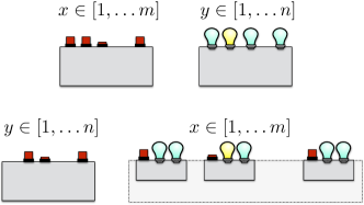
Figure 11: Top: Setup for the inference of measurements. Bottom: Setup for the inference of families of states.

The aim of data-driven inference is to infer the maximal noncommittal linear maps $M\mathrel{\mathop{\ordinarycolon}}\mathbb{R}^{l}\rightarrow\mathbb{R}^{n}$ consistent with $\{\mathbf{p}_{x}\}$, that is, the linear map $M$ that minimize the volume of $M(\mathbb{S})$ such that the range $M(\mathbb{S})$ contains the distributions $\{\mathbf{p}_{x}\}\subseteq\mathbb{R}^{n}$. We recall that $\mathbb{S}$ is the set of all states of the system of linear dimension $\ell$. As already noticed in the Main Text, not any linear transformation corresponds to a legitimate measurement: in case of a non physical inference $M$, failure is declared and a larger set $\{\mathbf{p}_{x}\}$ is required. This definition of the problem naturally identifies two steps: i) inferring the (possibly non unique) minimum-volume range $\hat{\mathcal{R}}$ consistent with $\{\mathbf{p}_{x}\}$, and ii) finding the measurements $\hat{M}$ whose range is $\hat{\mathcal{R}}$.

In the following definition we formalize the first of these two steps, that is, the inference process that consists of finding the minimum-volume range $M(\mathbb{S})$ such that $M(\mathbb{S})\supseteq\{\mathbf{p}_{x}\}$.

Definition 1 (Data-driven inference of measurements).

For any set $\{\mathbf{p}_{x}\}\subseteq\mathbb{R}^{n}$, we denote with $\operatorname{\mathtt{ddi}}(\{\mathbf{p}_{x}\}\;|\;\mathbb{S})$ the data-driven inference map

$$\operatorname{\mathtt{ddi}}\left(\left\{\mathbf{p}_{x}\right\}\;\big{|}\;\mathbb{S}\right)=\operatorname*{argmin}_{\begin{subarray}{c}M(\mathbb{S})\\ \{\mathbf{p}_{x}\}\subseteq M(\mathbb{S})\subseteq\operatorname{aff}\{\mathbf{p}_{x}\}\end{subarray}}\operatorname{\mathcal{V}}\left(M(\mathbb{S})\right),$$ (8)

where $\operatorname{\mathcal{V}}(\mathcal{R})$ denotes the Euclidean volume of $\mathcal{R}$ and the minimization is over subsets $M(\mathbb{S})$ corresponding to linear transformations of the set of states $\mathbb{S}$ that lie on the affine subspace generated by $\{\mathbf{p}_{x}\}$.

In general the outcome of the DDI map is not unique, and the map returns a set of ranges. We notice that, if the available prior information does not identify a unique set $\mathbb{S}$ of states, the set $\mathbb{S}$ itself can be considered as part of the optimization problem in the above definition, by taking the minimum of Eq. (8) over any possible $\mathbb{S}$.

We can now derive the main result of this section, that establishes the special role played by (hyper)-ellipsoidal sets $\mathbb{S}$ of states in the context of the DDI of measurements.

Before stating the main theorem we need the following definition.

Definition 2 ($\mathcal{U}$-symmetric set).

Given a set of transformations $\mathcal{U}$, and a set $\mathcal{X}\subseteq\mathbb{R}^{k}$, we say that $\mathcal{X}$ is $\mathcal{U}$-symmetric if $U(\mathcal{X})\mathrel{\mathop{\ordinarycolon}}=\{U\mathbf{x}|\mathbf{x}\in\mathcal{X}\}=\mathcal{X}$ for any $U\in\mathcal{U}$, where we have chosen a $k$-dimensional representation of the set $\mathcal{U}$.

Theorem 1.

Given a set of states $\mathbb{S}$ the following conditions are equivalent:

1. $\operatorname{\mathtt{ddi}}(\mathcal{X}|\mathbb{S})$ is a singleton for any $\mathcal{X}\subseteq\mathbb{R}^{n}$ and any $n\in\mathbb{N}$.

2. $\operatorname{\mathtt{ddi}}(\mathcal{X}|\mathbb{S})$ is $\mathcal{U}$-symmetric for any $\mathcal{U}$–symmetric $\mathcal{X}$, where $\mathcal{U}$ is a set of orthogonal matrices.

3. $\mathbb{S}$ is a (hyper)–ellipsoid.

Proof.

Let us prove each implication separately:

$\ref{item:singleton-sm}\Rightarrow\ref{item:symmetry-sm}$

Consider a $\mathcal{U}$–symmetric $\mathcal{X}$, and suppose by absurd that $\operatorname{\mathtt{ddi}}(\mathcal{X}|\mathbb{S})$ is a singleton $\mathcal{Y}$, but $\mathcal{Y}$ is not $\mathcal{U}$–symmetric. Then there exists $U\in\mathcal{U}$ such that $\mathcal{Y}^{\prime}\mathrel{\mathop{\ordinarycolon}}=\{U\mathbf{y}\;|\;\mathbf{y}\in\mathcal{Y}\}\neq\mathcal{Y}$. Since $\mathcal{Y}^{\prime}\supseteq\mathcal{X}$ and $\operatorname{\mathcal{V}}(\mathcal{Y}^{\prime})=\operatorname{\mathcal{V}}(\mathcal{Y})$, one has the absurd $\mathcal{Y}^{\prime}\in\operatorname{\mathtt{ddi}}(\mathcal{X}|\mathbb{S})$.

$\ref{item:symmetry-sm}\Rightarrow\ref{item:ellipsoid-sm}$

The implication follows from Lemma 1, by taking $\mathcal{X}$ to be a sphere and observing that $\{M(\mathbb{S})\,|\,M\in\mathfrak{M}_{{n}\times{\ell}})$ contains all spheres if and only if $\mathbb{S}$ is a (hyper)–ellipsoid.

$\ref{item:ellipsoid-sm}\Rightarrow\ref{item:singleton-sm}$

Follows immediately from Lemma 1, due to John’s uniqueness theorem for minimum–volume enclosing ellipsoids [43]. ∎

Notice that for (hyper)-ellipsoidal $\mathbb{S}$, for any $n\in\mathbb{N}$ and any $\mathcal{X}\subseteq\mathbb{R}^{n}$ one has

$$\operatorname{\mathtt{ddi}}(\mathcal{X}|\mathbb{S})=\left\{\operatorname{\mathtt{MVEE}}\left(\mathcal{X}\right)\right\},$$

where $\operatorname{\mathtt{MVEE}}(\mathcal{X})$ denotes the minimum–volume enclosing ellipsoid [45] for $\mathcal{X}$.

B.2 Inference of states

A setup comprising several boxes is given. One box is equipped with $n$ buttons, and the remaining $m$ boxes are equipped with one button and two light bulbs each. At each run of the experiment, Alice presses button $y$ of the former box, and selects box $x$ among the remaining boxes by pressing its button. She iterates this procedure many times, recording the frequencies $\{\mathbf{p}_{x}\}$ whose $y$-th element is the probability of the first bulb of box $x$ to light up given $y$. This situation is illustrated in the bottom part of Fig. 11.

The aim of data-driven inference is to infer the maximal noncommittal linear maps $R\mathrel{\mathop{\ordinarycolon}}\mathbb{R}^{l}\rightarrow\mathbb{R}^{n}$ consistent with $\{\mathbf{p}_{x}\}$, that is, the linear maps $R$ that minimize the volume of $R(\mathbb{E})$ such that the range $R(\mathbb{E})$ contains the distributions $\{\mathbf{p}_{x}\}\subseteq\mathbb{R}^{n}$. We recall that $\mathbb{E}$ is the set of all effects of the system of linear dimension $\ell$. Notice that not any linear map $R$ corresponds to a set of physical states: in case of a non physical inference $R$, failure is declared and a larger set $\{\mathbf{p}_{x}\}$ is required. This definition of the problem naturally identifies two steps: i) inferring the (possibly non unique) minimum-volume range $\hat{\mathcal{R}}$ consistent with $\{\mathbf{p}_{x}\}$, and ii) finding the linear transformations $\hat{R}$ whose range is $\hat{\mathcal{R}}$.

In the following definition we formalize the first of these two steps, that is, the inference process that consists of finding the minimum-volume range $R(\mathbb{E})$ such that $R(\mathbb{E})\supseteq\{\mathbf{p}_{x}\}$.

Definition 3 (Data-driven inference of states).

For any set $\{\mathbf{p}_{x}\}\subseteq\mathbb{R}^{n}$, we denote with $\operatorname{\mathtt{ddi}}(\{\mathbf{p}_{x}\}\;|\;\mathbb{E})$ the data-driven inference map

$$\operatorname{\mathtt{ddi}}\left(\left\{\mathbf{p}_{x}\right\}\;\big{|}\;\mathbb{E}\right)=\operatorname*{argmin}_{\begin{subarray}{c}R(\mathbb{E})\\ \{\mathbf{p}_{x},\mathbf{0},\mathbf{1}\}\subseteq R(\mathbb{E})\subseteq\operatorname{span}\{\mathbf{p}_{x},\mathbf{1}\}\\ R(e)=\mathbf{1}\end{subarray}}\operatorname{\mathcal{V}}\left(R(\mathbb{E})\right),$$ (9)

where the minimization is over subsets $R(\mathbb{E})\subseteq\mathbb{R}^{n}$ corresponding to linear transformations of the set of effects $\mathbb{E}$ that lie on the real span generated by $\{\mathbf{p}_{x}\}\cup\{\mathbf{1}\}$, and the two points $R(0)=\mathbf{0}=(0,0,\ldots,0)\in\mathbb{R}^{n}$, $R(e)=\mathbf{1}=(1,1,\ldots,1)\in\mathbb{R}^{n}$ are the images of the null effect $0\in\mathbb{E}$ and of the deterministic $e\in\mathbb{E}$ effect respectively (this last condition poses a not trivial linear constraint $R(e)=\mathbf{1}$).

In general the output of the DDI map is not unique, and the map returns a set. We notice that, if the available prior information does not identify a unique set $\mathbb{E}$ of effects, the set $\mathbb{E}$ itself can be considered as part of the optimization problem in the above definition, by taking the minimum of Eq. (9) over any possible $\mathbb{E}$.

In the definition of DDI of states, the set $\{\mathbf{p}_{x}\}$ has been extended to include the two points $\mathbf{0}=(0,0,\ldots,0)\in\mathbb{R}^{n}$ and $\mathbf{1}=(1,1,\ldots,1)\in\mathbb{R}^{n}$, corresponding to the null $0\in\mathbb{E}$ and to the deterministic effect $e\in\mathbb{E}$ respectively. This is so because the points $\mathbf{0}$ and $\mathbf{1}$, which could be uncollected by Alice, strongly characterize the geometry of the range $R(\mathbb{E})$ of the linear map $R$ (see also Fig. 10).

There are two main differences between the DDI of states and that of measurements given in Definition 1, when regarded as optimization problems. The first difference is in the set of points where the linear function to be inferred is applied. Indeed, in DDI of states the set $\mathbb{E}$ is not a strictly affine subspace of $\mathbb{R}^{l}$, while in DDI of measurements the convex set $\mathbb{S}$ is a strictly affine subspace of $\mathbb{R}^{l}$ of dimension $\ell-1$ (see also Fig. 10). Moreover, the fixed points of the linear map $R$ in the DDI of states introduce a further linear constraint $R(e)=\mathbf{p}_{e}$ to the optimization problem. Due to these differences we cannot provide a simple characterization of the DDI of states as for example the one in Theorem 1 for DDI of measurements. A more accurate geometrical analysis of the DDI map for states will be the subject of future research.

Appendix C Range inversion

In both cases of inference presented above the device to be inferred (either a measurement or a family of states) induces a linear map

$$D\mathrel{\mathop{\ordinarycolon}}\, \mathbb{R}^{\ell}\rightarrow\mathbb{R}^{n},$$ (10)

for some $n\in\mathbb{N}$.

We denote by $\mathcal{A}\in\mathbb{R}^{\ell}$ a subset of the domain of the map $D$ (this corresponds to the set of states $\mathcal{S}$ or the set of effects $\mathcal{E}$ in the inference protocol) and we denote by $D(\mathcal{A})\in\mathbb{R}^{n}$ the image of $\mathcal{A}$ via the map $D$ (this corresponds to the set of points $\{\mathbf{p}_{x}\}_{x=1}^{m}$ collected via the inference protocol):

$$D(\mathcal{A})\mathrel{\mathop{\ordinarycolon}}=\left\{D\mathbf{a}\;|\;\mathbf{a}\in\mathcal{A}\right\}.$$

Finally we denote the set of all linear transformations of $\mathcal{A}$ into $\mathbb{R}^{n}$ as

$$\mathcal{D}_{n}(\mathcal{A})\mathrel{\mathop{\ordinarycolon}}=\left\{D(\mathcal{A})\;|\;\forall D\in\mathfrak{M}_{{n}\times{\ell}}\;\right\}.$$ (11)

We can now introduce a notion of equivalence for maps $D$ based on the coincidence of their range $D(\mathbb{A})$.

Definition 4 (Equivalence).

For any $n\in\mathbb{N}$ and any $D\in\mathfrak{M}_{{n}\times{\ell}}$, we denote with $[D]$ the equivalence class

$$\left[D\right]\mathrel{\mathop{\ordinarycolon}}=\left\{D^{\prime}\in\mathfrak{M}_{{n}\times{\ell}}\;|\;D^{\prime}\left(\mathbb{A}\right)=D\left(\mathbb{A}\right)\right\}.$$

Notice that any two elements of $[D]$ do not necessarily share the same support.

In the Main Text we referred to any transformation $U$ that leaves a set $\mathbb{A}$ invariant, that is such that $U(\mathbb{A})=\mathbb{A}$, as a gauge symmetry. The following theorem shows that the equivalence class in Definition 4 is fully specified by the symmetries of $\mathbb{A}$.

Theorem 2.

For any $n\in\mathbb{N}$ and any $D\in\mathfrak{M}_{{n}\times{\ell}}$ one has

$$\left[D\right]=\left\{DU\;|\;\forall U\textrm{ s.t. }D^{+}DU\left(\mathbb{A}\right)=D^{+}D\left(\mathbb{A}\right)\right\}.$$ (12)

Proof.

The statement can be rephrased as follows. For any $D^{\prime}\in\mathfrak{M}_{{n}\times{\ell}}$ the following conditions are equivalent:

1. There exists $U\in\mathfrak{M}_{{n}\times{\ell}}$ such that $D^{\prime}=DU$ and $D^{+}DU(\mathbb{A})=D^{+}D(\mathbb{A})$.

2. $D^{\prime}\left(\mathbb{A}\right)=D\left(\mathbb{A}\right)$.

Let us prove each implication separately:

$\ref{item:symmetry}\Rightarrow\ref{item:equivalence}$

By hypothesis $U$ is such that $D^{+}DU(\mathbb{A})=D^{+}D(\mathbb{A})$. By multiplying both sides by $D$ from the left one has $DD^{+}DU(\mathbb{A})=DD^{+}D(\mathbb{A})$. Since $D=DD^{+}D$ one has $DU(\mathbb{A})=D(\mathbb{A})$. Hence the thesis.

$\ref{item:equivalence}\Rightarrow\ref{item:symmetry}$

Since by hypothesis $D^{\prime}(\mathbb{A})=D(\mathbb{A})$, one has $\operatorname{span}D^{\prime}(\mathbb{A})=\operatorname{span}D(\mathbb{A})$. Since by hypothesis $\operatorname{span}\mathbb{A}=\mathbb{R}^{\ell}$, one has $\operatorname{span}D(\mathbb{A})=\operatorname{rng}D$ and $\operatorname{span}D^{\prime}(\mathbb{A})=\operatorname{rng}D^{\prime}$. Hence, $\operatorname{rng}D=\operatorname{rng}D^{\prime}$, and thus $DD^{+}=D^{\prime}D^{\prime+}$. Then $D^{\prime}=D^{\prime}D^{\prime+}D^{\prime}=DD^{+}D^{\prime}$. By setting $U\mathrel{\mathop{\ordinarycolon}}=D^{+}D^{\prime}$ one has $DU(\mathbb{A})=D(\mathbb{A})$. By multiplying both sides by $D^{+}$ from the left one has $D^{+}DU(\mathbb{A})=D^{+}D(\mathbb{A})$. Hence the thesis. ∎

An immediate corollary of the theorem is:

Corollary 1.

For any $D$ such tat $D^{+}D=\openone$, due to Eq. (12) one has that any $D^{\prime}\in[D]$ is equivalent to $D$ up to a symmetry $U$ of the set $\mathbb{A}$.

Notice that if the map $D$ is for example the linear map associated to a measurement, the corollary states that for any informationally complete measurement $M$ the range $M(\mathbb{S})$ identifies $M$ up to gauge symmetries. This is the statement of Theorem 2 in the Main Text of the paper.

C.1 Measurement range inversion

In case of $(\ell-1)$–dimensional spherical $\mathbb{S}$ one can also explicitly derive all the linear transformations that correspond to any given (hyper)-ellipsoidal range. This is the content of the following proposition.

Proposition 1.

For $(\ell-1)$–dimensional unit–spherical $\mathbb{S}$, for any $n\in\mathbb{N}$ and any $D\in\mathfrak{M}_{{n}\times{\ell}}$, let $\mathbf{t}\mathrel{\mathop{\ordinarycolon}}=D\mathbf{u}$, let $T=D(\openone-\mathbf{u}\mathbf{u}^{T})$, and let $Q=TT^{T}$. One has

$$D\left(\mathbb{S}\right)=\left\{\mathbf{p}\;\Big{|}\;\begin{cases}(\openone-QQ^{+})(\mathbf{p}-\mathbf{t})=0\\ (\mathbf{p}-\mathbf{t})^{T}Q^{+}(\mathbf{p}-\mathbf{t})\leq 1\end{cases}\right\}.$$

Proof.

Due to Lemma 1, without loss of generality we take $\mathbb{S}$ to be the unit–sphere centered in $\mathbf{u}$ (centering in $\mathbf{u}$ might apparently require a translation of the sphere on the affine subspace, but a linear transformation suffices due to the Lemma; the inverse linear transformation can be performed on the effects, so without restriction one can consider the states centered in $\mathbf{u}$).

One has $\mathbf{a}\in\mathbb{S}$ if and only if $|\mathbf{a}-\mathbf{u}|_{2}\leq 1$ and $\mathbf{u}^{T}\mathbf{a}=1$. For any $\mathbf{a}\in\mathbb{S}$ one has $D\left(\mathbf{a}\right)=\mathbf{t}+T\mathbf{a}$. Hence

$$D\left(\mathbb{S}\right)=\left\{\mathbf{p}=\mathbf{t}+T\mathbf{a}\;\Big{|}\;\left|\mathbf{a}-\mathbf{u}\right|_{2}=1,\;\mathbf{u}^{T}\mathbf{a}=1\right\}.$$

Solutions of $T\mathbf{a}=\mathbf{p}-\mathbf{t}$ in variable $\mathbf{a}$ exist if and only if

$$TT^{+}(\mathbf{p}-\mathbf{t})=\mathbf{p}-\mathbf{t}.$$ (13)

Since $T^{+}T$ and $\mathbf{u}\mathbf{u}^{T}$ are orthogonal projectors by construction, solutions are given by

$$\mathbf{a}=T^{+}\left(\mathbf{p}-\mathbf{t}\right)+\lambda\mathbf{u}+\left(\openone-T^{+}T-\mathbf{u}\mathbf{u}^{T}\right)\mathbf{v},$$

for any scalar $\lambda$ and any vector $\mathbf{v}$.

Condition $\mathbf{u}^{T}\mathbf{a}=1$ imposes $\lambda=1$. For any vector $\mathbf{v}$ such that $|\mathbf{a}|_{2}\leq 1$, the same condition is also verified for $\mathbf{v}=0$. Since $D(\mathbf{a})$ is independent of $\mathbf{v}$, without loss of generality we take $\mathbf{v}=0$.

Therefore one has

$$D\left(\mathbb{S}\right)=\left\{\mathbf{p}\;\Big{|}\;\begin{cases}(\openone-TT^{+})(\mathbf{p}-\mathbf{t})=0,\\ (\mathbf{p}-\mathbf{t})^{T}{T^{+}}^{T}T^{+}(\mathbf{p}-\mathbf{t})\leq 1.\end{cases}\right\}.$$

By the elementary properties of the Moore-Penrose pseudoinverse, one immediately has that $TT^{+}=QQ^{+}$ and ${T^{+}}^{T}T^{+}=Q^{+}$. Hence the statement follows. ∎

Appendix D Data-driven reconstruction

D.1 Data-driven reconstruction of measurements

In the protocol of data-driven reconstruction of measurements, an experimentalist, say Bob, is in charge of building the state-preparator $\mathcal{S}$ corresponding to the box equipped with buttons in the upper part of Fig. 12. His aim is to enable Alice to correctly infer measurement $M$, corresponding to the box with light bulbs, up to the equivalence of Theorem 2. In this case, we say that $\mathcal{S}$ is observationally complete for $M$.

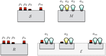
Figure 12: Top: Setup for the data-driven reconstruction of measurements. On the right is a measurement $\{a_{y}\}_{y=1}^{n}$, that can be thought as a box $M$ equipped with $n$ bulbs, one for each effect $a_{y}\in\mathbb{E}$, $y=1,2,\ldots,n$, corresponding to the possible outcomes of the measurement. On the left is a state preparator that can be thought as a box with $m$ possible buttons, each button corresponding to a state $\rho_{x}\in\mathbb{S}$, $x=1,\ldots,m$. At each run of the experiment a button is pressed and the outcome of the measurements is recorded. We iterate this procedure many times recording the frequencies $p_{x}^{y}$ that are our estimates of the probabilities $a_{y}(\rho_{x})$. Since each state $\rho_{x}\in\mathbb{S}$ can be regarded as a vector in $\mathbb{R}^{\ell}$, the whole experiment can be represented by a linear map $M\mathrel{\mathop{\ordinarycolon}}\mathbb{R}^{l}\rightarrow\mathbb{R}^{n}$, with $\rho_{x}\mapsto\mathbf{p}_{x}$, $p_{x}^{y}\mathrel{\mathop{\ordinarycolon}}=a_{y}(\rho_{x})$. Any state in the set $\mathcal{S}=\{\rho_{x}\}_{x=1}^{m}$ is associated with a point $\mathbf{p}_{x}\in\mathbb{R}^{n}$. Bottom: Setup for the data-driven reconstruction of families of states. On the left is a state preparator $R$ that can prepare one out of a finite set $\{\rho_{y}\}_{y=1}^{n}$ of states. We can think of an $n$-buttons state preparator: whenever we press the button $y$ the state $\rho_{y}$ is prepared. On the right is a measurement box with $m$ possible buttons: whenever button $x$ (with $x=1,\ldots,m$) is pressed the two outcomes measurement described by the pair of effects $\{a_{x},\bar{a}_{x}\}$ is applied to the prepared state. Give a state $\rho_{y}$ the outcome $a_{x}$ will be obtained with probability $a_{x}(\rho_{y})$ (clearly, $a_{x}(\rho_{y})+\bar{a}_{x}(\rho_{y})=1$). We iterate this procedure for all the $n$ states $\rho_{y}$ and the $m$ measurements $\{a_{x},\bar{a}_{x}\}$, thus recording the frequencies $p^{y}_{x}$, which are our estimate of the probabilities $a_{x}(\rho_{y})$. Since each effect $a_{x}$ corresponds to a vector in $\mathbb{R}^{\ell}$, the whole experiment can be represented by a linear map $R\mathrel{\mathop{\ordinarycolon}}\mathbb{R}^{l}\to\mathbb{R}^{n}$, with $a_{x}\mapsto\mathbf{p}_{x}$, ${p}^{y}_{x}\mathrel{\mathop{\ordinarycolon}}=a_{x}(\rho_{y})$. Any effect in the set $\mathcal{E}=\{a_{x}\}_{x=1}^{m}$ is associated with a point $\mathbf{p}_{x}\in\mathbb{R}^{n}$.

Definition 5 (Observational complete set of states).

Let $\{\mathbb{S},\mathbb{E}\}$ be a physical system of linear dimension $\ell$ and $M\in\mathfrak{M}_{{n}\times{\ell}}$ be a measurement. A set of states $\mathcal{S}\subseteq\mathbb{S}$ is observationally complete for $M$ if and only if

$$\operatorname{\mathtt{ddi}}(M\left(\mathcal{S}\right)|\mathbb{S})=M\left(\mathbb{S}\right)$$ (14)

where $\operatorname{\mathtt{ddi}}$ is the data driven inference of measurements.

The following result shows that the notion of observational completeness depends only on the support of $M$.

Theorem 3.

Let $\{\mathbb{S},\mathbb{E}\}$ be a physical system of linear dimension $\ell$ and let $\mathcal{S}\subseteq\mathbb{S}$ be a set of states. Let $\mathcal{V}$ be a linear subspace of $\mathbb{R}^{\ell}$ and let $\Pi$ denote the projector on $\mathcal{V}$. Then $\mathcal{S}$ is observationally complete for $\Pi$ if and only if it is observationally complete for any $M\in\mathfrak{M}_{{n}\times{\ell}}$ such that $\operatorname{supp}M=\mathcal{V}$, i.e.

$$\begin{aligned} &\operatorname{\mathtt{ddi}}(\Pi\left(\mathcal{S}\right)|\mathbb{S})=\Pi\left(\mathbb{S}\right)\iff\\ &\operatorname{\mathtt{ddi}}(M\left(\mathcal{S}\right)|\mathbb{S})=M\left(\mathbb{S}\right)\;\forall M\mbox{ s.t. }\operatorname{supp}M=\mathcal{V}.\end{aligned}$$ (15)

Proof.

We only need to prove the $\implies$ direction since the opposite one is trivially true. Let us then suppose that $\operatorname{\mathtt{ddi}}(\Pi\left(\mathcal{S}\right)|\mathbb{S})=\Pi\left(\mathbb{S}\right)$ and let us fix an arbitrary $M\in\mathfrak{M}_{{n}\times{\ell}}$ such that $\operatorname{supp}M=\mathcal{V}$. Then we have $M\Pi=M$. By using lemma 2 we have

$$\begin{aligned} &\operatorname{\mathtt{ddi}}(M\left(\mathcal{S}\right)|\mathbb{S})=\operatorname{\mathtt{ddi}}(M\Pi\left(\mathcal{S}\right)|\mathbb{S})=\\ &M\operatorname{\mathtt{ddi}}(\Pi\left(\mathcal{S}\right)|\mathbb{S})=M\Pi\left(\mathbb{S}\right)=M\left(\mathbb{S}\right)\end{aligned}$$

and the thesis is proved. ∎

An immediate corollary of this theorem is:

Corollary 2.

A set of states $\mathcal{S}\subseteq\mathbb{S}$ is observationally complete for any informationally complete measurement if and only if $\operatorname{\mathtt{ddi}}(\mathcal{S}|\mathbb{S})=\mathbb{S}$.

This is the statement of Theorem 3 in the Main Text.

If the set of states $\mathbb{S}$ is (hyper)-spherical, it is possible to give an explicit characterization of the sets of states with minimum cardinality that are observationally complete for the informationally complete measurements.

Proposition 2.

Let $\{\mathbb{S},\mathbb{E}\}$ be a physical system of linear dimension $\ell$ and let $\mathbb{S}$ be an $(\ell-1)$-dimensional (hyper)-sphere. Then the following conditions are equivalent:

1. $\mathcal{S}$ is a regular $(\ell-1)$–simplex inscribed in $\mathbb{S}$.

2. $\operatorname{\mathtt{ddi}}(\mathcal{S}|\mathbb{S})=\mathbb{S}$ and $\mathcal{S}$ has minimal cardinality.

Proof.

Let us prove each implication separately:

1 $\Rightarrow$ 2

Let $\mathcal{A}$ be the regular $(\ell-1)$–simplex inscribed in $\mathbb{A}$. It is known [46] that $\operatorname{\mathtt{MVEE}}(\mathcal{A})=\mathbb{A}$.

2 $\Rightarrow$ 1

Since $\mathbb{S}$ is (hyper)-spherical $\operatorname{\mathtt{ddi}}(\mathcal{S}|\mathbb{S})=\operatorname{\mathtt{MVEE}}(\mathcal{S})=\mathbb{S}$. Then $\operatorname{\mathtt{MVEE}}(\mathcal{S})$ is the smallest (hyper)-sphere which contains $\mathcal{S}$. Clearly the cardinality of $\mathcal{S}$ must be greater then $\ell$. On the other hand, as the proof of the previous item shows, the regular simplex has cardinality $\ell$ and is observationally complete. Therefore $\mathcal{S}$ must be a simplex. We now show that $\mathcal{S}$ is regular. Let us denote with $\operatorname{conv}(\mathcal{S})$ the convex hull of $\mathcal{S}$ and let $r_{max}$ be the radius of the largest sphere inscribed in $\operatorname{conv}(\mathcal{S})$. Since $\operatorname{\mathtt{MVEE}}(\mathcal{S})\subseteq(\ell-1)\operatorname{conv}(\mathcal{S})$ [44] we have $(\ell-1)r_{max}\geq R$ where $R$ is the radius of $\operatorname{\mathtt{MVEE}}(\mathcal{S})$. On the other hand, we have $(\ell-1)r_{max}\leq R$ from Euler inequality  [47]. Therefore $(\ell-1)r_{max}=R$ which holds if and only if the simplex is regular. ∎

Let us consider the case when $\ell=3$ and hence $\mathbb{S}$ is a circle. In this case, any regular polygon $\mathcal{S}$ with $n$ vertices inscribed in $\mathbb{A}$ is $\mathcal{U}$–symmetric, where $\mathcal{U}$ is an orthogonal representation of the dihedral group. Since for $n\geq 3$, the only $\mathcal{U}$–symmetric ellipse is the circle, due to Theorem 1 and Corollary 2 any such an $\mathcal{S}$ is observationally complete for any informationally complete measurement.

Let us now consider the case when $\ell=4$ and hence $\mathbb{S}$ is a sphere. In this case, any Platonic solid with $n$ vertices inscribed in $\mathbb{S}$ is $\mathcal{U}$-symmetric, where $\mathcal{U}$ is an orthogonal representation of the tetrahedral (for tetrahedra), octahedral (for octahedra and cubes), or icosahedral (for icosahedra or dodecahedra) group. Since the only $\mathcal{U}$–symmetric ellipsoid is the sphere, due to Theorem 1 and Corollary 2 any such an $\mathcal{S}$ is observationally complete for any informationally complete measurement.

D.2 Data-driven reconstruction of states

In the protocol of data-driven reconstruction of family of states, Bob is in charge of building the tests (binary-outcome measurements) $\mathcal{E}$ corresponding to the boxes equipped with one button and two light bulbs each in the lower part of Fig. 12. His aim is to enable Alice to correctly infer the family of states $R$, corresponding to the box with $n$ buttons, up to the equivalence of Theorem 2. In this case, we say that $\mathcal{E}$ is observationally complete for $R$.

Definition 6 (Observational complete set of effects).

Let $\{\mathbb{S},\mathbb{E}\}$ be a physical system of linear dimension $\ell$ and $R\in\mathfrak{M}_{{n}\times{\ell}}$ be a family of states. A set of effects $\mathcal{E}\subseteq\mathbb{E}$ is observationally complete for $R$ if and only if

$$\operatorname{\mathtt{ddi}}(R\left(\mathcal{E}\right)|\mathbb{E})=R\left(\mathbb{E}\right)$$ (16)

where $\operatorname{\mathtt{ddi}}$ is the data driven inference of states.

Clearly, the analogous of theorem 3 holds

Theorem 4.

Let $\{\mathbb{R},\mathbb{E}\}$ be a physical system of linear dimension $\ell$ and let $\mathcal{E}\subseteq\mathbb{E}$ be a set of effects. Let $\mathcal{V}$ be a linear subspace of $\mathbb{R}^{\ell}$ and let $\Pi$ denote the projector on $\mathcal{V}$. Then $\mathcal{E}$ is observationally complete for $\Pi$ if and only of it is observationally complete for any $R\in\mathfrak{M}_{{n}\times{\ell}}$ such that $\operatorname{supp}R=\mathcal{V}$, i.e.

$$\begin{aligned} &\operatorname{\mathtt{ddi}}(\Pi\left(\mathcal{E}\right)|\mathbb{E})=\Pi\left(\mathbb{E}\right)\iff\\ &\operatorname{\mathtt{ddi}}(R\left(\mathcal{E}\right)|\mathbb{E})=R\left(\mathbb{E}\right)\;\forall R\mbox{ s.t. }\operatorname{supp}R=\mathcal{V}.\end{aligned}$$ (17)

Proof.

The proof of this result is completely analogous to the proof of Theorem 3. ∎

Appendix E Technical Lemmas

E.1 Affine transformations of a strictly affine set

For any $n\in\mathbb{N}$, any $D\in\mathfrak{M}_{{n}\times{\ell}}$, and any $\mathbf{d}\in\mathbb{R}^{n}$, let $\mathcal{F}_{D,\mathbf{d}}\mathrel{\mathop{\ordinarycolon}}\mathbb{R}^{\ell}\to\mathbb{R}^{n}$ denote the affine map such that for any $\mathbf{a}\in\mathbb{R}^{\ell}$ one has

$$\mathcal{F}_{D,\mathbf{d}}(\mathbf{a})\mathrel{\mathop{\ordinarycolon}}=D\mathbf{a}+\mathbf{d}.$$

For any set $\mathcal{A}\subseteq\mathbb{R}^{\ell}$ we adopt the set builder notation

$$\mathcal{F}_{D,\mathbf{d}}\left(\mathcal{A}\right)\mathrel{\mathop{\ordinarycolon}}=\left\{\mathcal{F}_{D,\mathbf{d}}\left(\mathbf{a}\right)\;|\;\mathbf{a}\in\mathcal{A}\right\}.$$

For any $n\in\mathbb{N}$ and any $\mathcal{A}\subseteq\mathbb{R}^{\ell}$, let $\mathcal{F}_{n}(\mathcal{A})$ denote the set of all affine transformations of $\mathcal{A}$ into $\mathbb{R}^{n}$, that is

$$\mathcal{F}_{n}\left(\mathcal{A}\right)\mathrel{\mathop{\ordinarycolon}}=\left\{\mathcal{F}_{D,\mathbf{d}}\left(\mathcal{A}\right)\;\Big{|}\;\forall D\in\mathfrak{M}_{{n}\times{\ell}},\;\forall\mathbf{d}\in\mathbb{R}^{n}\;\right\}.$$

We say that an affine subspace is strictly affine if and only if it is not a linear subspace. For any $n\in\mathbb{N}$ and any $\mathcal{X}\in\mathbb{R}^{n}$, let $\operatorname{aff}\mathcal{X}$ denote the affine hull of $\mathcal{X}$. Let $\mathbf{u}\in\operatorname{aff}\mathbb{A}$ denote the vector orthogonal to $\operatorname{aff}\mathbb{A}$. Without loss of generality we take $\mathbf{u}$ such that $|\mathbf{u}|_{2}=1$.

Lemma 1.

For any $n\in\mathbb{N}$ and any $\mathbb{A}$ subset of a strictly affine subspace of $\mathbb{R}^{\ell}$ one has

$$\mathcal{D}_{n}\left(\mathbb{A}\right)=\mathcal{F}_{n}\left(\mathbb{A}\right).$$

(see Eq. (11) for the definition of $\mathcal{D}_{n}$.)

Proof.

Of course $\mathcal{D}_{n}(\mathbb{A})\subseteq\mathcal{F}_{n}(\mathbb{A})$, so we only need to prove the inverse inclusion. For any $D\in\mathfrak{M}_{{n}\times{\ell}}$ and $\mathbf{d}\in\mathbb{R}^{n}$, one has that $D^{\prime}\mathrel{\mathop{\ordinarycolon}}=D+\mathbf{d}\mathbf{u}^{T}$ is such that $\mathcal{F}_{D,\mathbf{d}}(a)=D^{\prime}(a)$ for any $a\in\mathbb{A}$. Hence the thesis follows. ∎

E.2 Commutativity of the DDI map

Lemma 2.

Let $D\in\mathfrak{M}_{{n}\times{\ell}}$, and $\mathcal{A}\subseteq\mathbb{R}^{\ell}$ such that $\mathcal{A}\subseteq\operatorname{supp}D$ one has

$$D(\operatorname{\mathtt{ddi}}(\mathcal{A}|\mathbb{A}))=\operatorname{\mathtt{ddi}}(D(\mathcal{A})|\mathbb{A}).$$ (18)

Proof.

By definition, the l.h.s. and r.h.s. of Eq. (18) are given by, respectively,

$$D(\operatorname{\mathtt{ddi}}(\mathcal{A}|\mathbb{A})) \mathrel{\mathop{\ordinarycolon}}=D(\operatorname*{argmin}_{\mathcal{X}\in\mathfrak{X}}\operatorname{\mathcal{V}}(\mathcal{X})),$$

$$\operatorname{\mathtt{ddi}}(D(\mathcal{A})|\mathbb{A}) \mathrel{\mathop{\ordinarycolon}}=\operatorname*{argmin}_{\mathcal{Y}\in\mathfrak{Y}}\operatorname{\mathcal{V}}(\mathcal{Y}),$$

with

$$\mathfrak{X} \mathrel{\mathop{\ordinarycolon}}=\{\mathcal{X}\in\mathcal{D}_{\ell}\left(\mathbb{A}\right)\;|\;\mathcal{A}\subseteq\mathcal{X}\subseteq\operatorname{aff}\mathcal{A}\},$$

$$\mathfrak{Y} \mathrel{\mathop{\ordinarycolon}}=\{\mathcal{Y}\in\mathcal{D}_{n}\left(\mathbb{A}\right)\;|\;D\left(\mathcal{A}\right)\subseteq\mathcal{Y}\subseteq\operatorname{aff}D\left(\mathcal{A}\right)\}.$$

The map $D$ is bijective from $\mathfrak{X}$ to $\mathfrak{Y}$. This can be easily seen as follows. Since $\mathcal{A}\subseteq\operatorname{supp}D$, by definition of $\mathfrak{X}$ for any $\mathcal{X}\in\mathfrak{X}$ one has $\mathcal{X}\subseteq\operatorname{supp}D$. Also, by definition of $\mathfrak{Y}$ for any $\mathcal{Y}\in\mathfrak{Y}$ one has $\mathcal{Y}\subseteq\operatorname{supp}D^{+}$. Moreover, $D$ preserves the ordering induced by function $\operatorname{\mathcal{V}}$, that is:

$$\operatorname{\mathcal{V}}\left(\mathcal{X}\right)=\lambda_{D}\operatorname{\mathcal{V}}\left(\mathcal{L}_{D}\left(\mathcal{X}\right)\right)\quad\forall\mathcal{X}\in\mathfrak{X},$$

for some $\lambda_{D}>0$ that only depends on $D$. Hence the statement follows. ∎

References

- Ozawa [1980] M. Ozawa, Optimal measurements for general quantum systems, Reports on Mathematical Physics 18, 11 (1980).
- Buscemi et al. [2005] F. Buscemi, M. Keyl, G. M. D’Ariano, P. Perinotti, and R. F. Werner, Clean positive operator valued measures, Journal of Mathematical Physics 46, 082109 (2005), https://doi.org/10.1063/1.2008996 .
- Blackwell [1953] D. Blackwell, Equivalent comparisons of experiments, The Annals of Mathematical Statistics 24, 265 (1953).
- Buscemi [2012] F. Buscemi, Comparison of quantum statistical models: Equivalent conditions for sufficiency, Communications in Mathematical Physics 310, 625 (2012).
- Marshall et al. [1979] A. W. Marshall, I. Olkin, and B. C. Arnold, Inequalities: theory of majorization and its applications, Vol. 143 (Springer, 1979).
- Torgersen [1991] E. Torgersen, Comparison of Statistical Experiments, Encyclopedia of Mathematics and its Applications (Cambridge University Press, 1991).
- Cohen et al. [1998] J. Cohen, J. H. Kempermann, and G. Zbaganu, Comparisons of Stochastic Matrices with Applications in Information Theory, Statistics, Economics and Population (Springer Science & Business Media, 1998).
- Lieb and Yngvason [1999] E. H. Lieb and J. Yngvason, The physics and mathematics of the second law of thermodynamics, Physics Reports 310, 1 (1999).
- Buscemi and Datta [2016] F. Buscemi and N. Datta, Equivalence between divisibility and monotonic decrease of information in classical and quantum stochastic processes, Phys. Rev. A 93, 012101 (2016).
- Gour et al. [2018] G. Gour, D. Jennings, F. Buscemi, R. Duan, and I. Marvian, Quantum majorization and a complete set of entropic conditions for quantum thermodynamics, Nature Communications 9, 5352 (2018).
- Dahl [1999] G. Dahl, Matrix majorization, Linear Algebra and its Applications 288, 53 (1999).
- Shmaya [2005] E. Shmaya, Comparison of information structures and completely positive maps, Journal of Physics A: Mathematical and General 38, 9717 (2005).
- Shannon [1958] C. E. Shannon, A note on a partial ordering for communication channels, Information and Control 1, 390 (1958).
- Korner [1977] J. Korner, Comparison of two noisy channels, Topics in information theory , 411 (1977).
- Liese and Miescke [2007] F. Liese and K.-J. Miescke, Statistical decision theory, in Statistical Decision Theory (Springer, 2007) pp. 1–52.
- Csiszar and Körner [2011] I. Csiszar and J. Körner, Information theory: coding theorems for discrete memoryless systems (Cambridge University Press, 2011).
- Luis and Sánchez-Soto [1999] A. Luis and L. L. Sánchez-Soto, Complete characterization of arbitrary quantum measurement processes, Phys. Rev. Lett. 83, 3573 (1999).
- D’Ariano and Lo Presti [2001] G. M. D’Ariano and P. Lo Presti, Quantum tomography for measuring experimentally the matrix elements of an arbitrary quantum operation, Phys. Rev. Lett. 86, 4195 (2001).
- D’Ariano et al. [2004] G. M. D’Ariano, L. Maccone, and P. L. Presti, Quantum calibration of measurement instrumentation, Phys. Rev. Lett. 93, 250407 (2004).
- Fiurášek [2001] J. Fiurášek, Maximum-likelihood estimation of quantum measurement, Physical Review A 64, 024102 (2001).
- Bisio et al. [2009] A. Bisio, G. Chiribella, G. M. D’Ariano, S. Facchini, and P. Perinotti, Optimal quantum tomography of states, measurements, and transformations, Phys. Rev. Lett. 102, 010404 (2009).
- Lundeen et al. [2009] J. Lundeen, A. Feito, H. Coldenstrodt-Ronge, K. Pregnell, C. Silberhorn, T. Ralph, J. Eisert, M. Plenio, and I. Walmsley, Tomography of quantum detectors, Nature Physics 5, 27 (2009).
- Feito et al. [2009] A. Feito, J. Lundeen, H. Coldenstrodt-Ronge, J. Eisert, M. B. Plenio, and I. A. Walmsley, Measuring measurement: theory and practice, New Journal of Physics 11, 093038 (2009).
- Spekkens [2007] R. W. Spekkens, Evidence for the epistemic view of quantum states: A toy theory, Phys. Rev. A 75, 032110 (2007).
- Popescu and Rohrlich [1994] S. Popescu and D. Rohrlich, Quantum nonlocality as an axiom, Foundations of Physics 24, 379 (1994).
- Barrett [2007] J. Barrett, Information processing in generalized probabilistic theories, Phys. Rev. A 75, 032304 (2007).
- Barrett et al. [2005] J. Barrett, N. Linden, S. Massar, S. Pironio, S. Popescu, and D. Roberts, Nonlocal correlations as an information-theoretic resource, Phys. Rev. A 71, 022101 (2005).
- Popescu [2014] S. Popescu, Nonlocality beyond quantum mechanics, Nature Physics 10, 264 EP (2014).
- D’Ariano and Tosini [2010] G. M. D’Ariano and A. Tosini, Testing axioms for quantum theory on probabilistic toy-theories, Quantum Information Processing 9, 95 (2010).
- D’Ariano et al. [2017] G. M. D’Ariano, G. Chiribella, and P. Perinotti, Quantum Theory from First Principles: An Informational Approach (Cambridge University Press, 2017).
- Hardy [2001] L. Hardy, Quantum theory from five reasonable axioms, Arxiv preprint quant-ph/0101012 (2001).
- Dakic and Brukner [2011] B. Dakic and C. Brukner, Quantum theory and beyond: is entanglement special?, in Deep Beauty: Understanding the Quantum World through Mathematical Innovation, edited by H. Halvorson (Cambridge University Press, 2011) pp. 365–392.
- Masanes and Müller [2011] L. Masanes and M. P. Müller, A derivation of quantum theory from physical requirements, New Journal of Physics 13, 063001 (2011).
- Chiribella et al. [2011] G. Chiribella, G. D’Ariano, and P. Perinotti, Informational derivation of quantum theory, Phys. Rev. A 84, 012311 (2011).
- Renes et al. [2004] J. M. Renes, R. Blume-Kohout, A. J. Scott, and C. M. Caves, Symmetric informationally complete quantum measurements, Journal of Mathematical Physics 45, 2171 (2004), https://doi.org/10.1063/1.1737053 .
- Zauner [2011] G. Zauner, Grundzüge einer nichtkommutativen Designtheorie, Ph.D. thesis, PhD thesis, University of Vienna, 1999. Published in English translation … (2011).
- Fuchs et al. [2017] C. Fuchs, M. Hoang, and B. Stacey, The sic question: History and state of play, Axioms 6, 21 (2017).
- Fuchs and Schack [2013] C. A. Fuchs and R. Schack, Quantum-bayesian coherence, Rev. Mod. Phys. 85, 1693 (2013).
- Mermin [2014] N. D. Mermin, Physics: Qbism puts the scientist back into science, Nature News 507, 421 (2014).
- Fuchs et al. [2014] C. A. Fuchs, N. D. Mermin, and R. Schack, An introduction to qbism with an application to the locality of quantum mechanics, American Journal of Physics 82, 749 (2014), https://doi.org/10.1119/1.4874855 .
- Dall’Arno et al. [2017] M. Dall’Arno, S. Brandsen, F. Buscemi, and V. Vedral, Device-independent tests of quantum measurements, Phys. Rev. Lett. 118, 250501 (2017).
- Buscemi and Dall’Arno [2019] F. Buscemi and M. Dall’Arno, Device-independent inference of physical devices: Theory and implementation, New J. Phys. 21, 113029 (2019).
- John [2014] F. John, Extremum problems with inequalities as subsidiary conditions, in Traces and Emergence of Nonlinear Programming, edited by G. Giorgi and T. H. Kjeldsen (Springer Basel, Basel, 2014) pp. 197–215.
- Boyd and Vandenberghe [2004] S. Boyd and L. Vandenberghe, Convex optimization (Cambridge university press, 2004).
- Todd [2016] M. J. Todd, Minimum-volume ellipsoids: Theory and algorithms, Vol. 23 (SIAM, 2016).
- Vandev [1992] D. Vandev, A minimal volume ellipsoid around a simplex, Comptes rendus de l’Académie bulgare des sciences: sciences mathématiques et naturelles 45, 37 (1992).
- Vince [2008] A. Vince, A simplex contained in a sphere, Journal of Geometry 89, 169 (2008).
- J.Todd and Yildirim [2007] M. J.Todd and E. A. Yildirim, On khachiyan’s algorithm for the computation of minimum-volume enclosing ellipsoids, Discrete Applied Mathematics 155, 1731 (2007).