A theoretical analysis of the doubly radiative decays $\eta^{(\prime)}\to\pi^{0}\gamma\gamma$ and $\eta^{\prime}\to\eta\gamma\gamma$

Abstract

The scalar and vector meson exchange contributions to the doubly radiative decays $\eta^{(\prime)}\to\pi^{0}\gamma\gamma$ and $\eta^{\prime}\to\eta\gamma\gamma$ are analysed within the Linear Sigma Model and Vector Meson Dominance frameworks, respectively. Predictions for the diphoton invariant mass spectra and the associated integrated branching ratios are given and compared with current available experimental data. Whilst a satisfactory description of the shape of the $\eta\to\pi^{0}\gamma\gamma$ and $\eta^{\prime}\to\pi^{0}\gamma\gamma$ decay spectra is obtained, thus supporting the validity of the approach, the corresponding branching ratios cannot be reproduced simultaneously. A first theoretical prediction for the recently measured $\eta^{\prime}\to\eta\gamma\gamma$ by the BESIII collaboration is also presented.

I Introduction

Measurements of $\eta$ and $\eta^{\prime}$ decays have reached unprecedented precision over the years placing new demands on the accuracy of the corresponding theoretical descriptions [1]. Amongst them, the doubly radiative decay $\eta\to\pi^{0}\gamma\gamma$ has attracted much interest as this reaction is a perfect laboratory for testing Chiral Perturbation Theory and its natural extensions, but also as a result of the decades-long tension between the associated theoretical predictions and the experimental measurements.

Likewise, the study of the $\eta^{\prime}\to\pi^{0}\gamma\gamma$ and $\eta^{\prime}\to\eta\gamma\gamma$ decay processes are of interest for a number of reasons. First, they complete existing calculations of the sister process $\eta\to\pi^{0}\gamma\gamma$, which has been studied in many different frameworks, ranging from the seminal works based on Vector Meson Dominance (VMD) [2, 3] and Chiral Perturbation Theory (ChPT) [4], to more modern treatments based on the unitarisation of the chiral amplitudes [5, 6] or dispersive formalisms [7]. At present, whilst there is only a course estimation for the branching ratio of the $\eta^{\prime}\to\pi^{0}\gamma\gamma$ decay [8, 9], there is no calculation or theoretical prediction for the $\eta^{\prime}\to\eta\gamma\gamma$ branching ratio. Second, the BESIII collaboration has recently reported the first measurements for the decays $\eta^{\prime}\to\pi^{0}\gamma\gamma$ [10] and $\eta^{\prime}\to\eta\gamma\gamma$ [11], thus, making the topic of timely interest [12]. Third, the analysis of these decays could help extract relevant information on the properties of the lowest-lying scalar resonances, in particular, the isovector $a_{0}(980)$ from the two $\eta^{(\prime)}\to\pi^{0}\gamma\gamma$ processes and the isoscalars $\sigma(500)$ and $f_{0}(980)$ from the $\eta^{\prime}\to\eta\gamma\gamma$ decay, thus, complementing other investigations such as the studies of $V\to P^{0}P^{0}\gamma$ decays ($V=\rho^{0},\omega,\phi$ and $P^{0}=\pi^{0},\eta)$ [13], $D$ and $J/\psi$ decays, central production, etc. (see note on scalar mesons in Ref. [14]). For all these reasons, the aim of the present work is to provide a first detailed evaluation of the invariant mass spectrum and integrated branching ratio for the three doubly radiative decays $\eta^{(\prime)}\to\pi^{0}\gamma\gamma$ and $\eta^{\prime}\to\eta\gamma\gamma$. Very preliminary results were presented in Refs. [15, 16].

On the experimental front, the branching ratio (BR) of the $\eta\to\pi^{0}\gamma\gamma$ decay has been measured by GAMS-2000 [17], $\mbox{BR}=(7.1\pm 1.4)\times 10^{-4}$, CrystalBall@AGS in 2005 [18], $\mbox{BR}=(3.5\pm 0.7\pm 0.6)\times 10^{-4}$, and 2008 [19], $\mbox{BR}=(2.21\pm 0.24\pm 0.47)\times 10^{-4}$, where the latter also included an invariant mass spectrum for the two outgoing photons. An independent analysis of the last CrystalBall data resulted in $\mbox{BR}=(2.7\pm 0.9\pm 0.5)\times 10^{-4}$ [20]. Early results are summarised in the review of Ref. [21]. Surprisingly low in comparison with all previous measurements is the 2006 result reported by the KLOE collaboration [22], $\mbox{BR}=(0.84\pm 0.27\pm 0.14)\times 10^{-4}$, based on a sample of $68\pm 23$ events. More recently, a new measurement of the diphoton energy spectrum, as well as new and more precise values for $\Gamma(\eta\to\pi^{0}\gamma\gamma)=(0.330\pm 0.030)$ eV and $\mbox{BR}=(2.54\pm 0.27)\times 10^{-4}$ have been released by the A2 collaboration at the Mainz Microtron (MAMI), based on the analysis of $1.2\times 10^{3}$ $\eta\to\pi^{0}\gamma\gamma$ decay events [23]. The latest PDG states a fit value of $\mbox{BR}=(2.56\pm 0.22)\times 10^{-4}$ [14]. For the $\eta^{\prime}\to\pi^{0}\gamma\gamma$ decay, the BESIII collaboration has recently reported for the first time the associated $m_{\gamma\gamma}^{2}$ invariant mass distribution [10]. The measured branching fraction is $\mbox{BR}=(3.20\pm 0.07\pm 0.23)\times 10^{-3}$, superseding the upper limit $\mbox{BR}<8\times 10^{-4}$ at 90% CL determined by the GAMS-2000 experiment [24]. Finally, for the $\eta^{\prime}\to\eta\gamma\gamma$ decay, a measurement of $\mbox{BR}<1.33\times 10^{-4}$ at 90% CL has been provided, again for the first time, by the BESIII collaboration [11].

On the theoretical front, the $\eta\to\pi^{0}\gamma\gamma$ decay has been a stringent test for the predictive power of ChPT. Within this framework, the tree-level contributions at ${\cal O}(p^{2})$ and ${\cal O}(p^{4})$ vanish because the pseudoscalar mesons involved are neutral. The first non-vanishing contribution comes at ${\cal O}(p^{4})$, either from kaon loops, largely suppressed by their mass, or from pion loops, also suppressed since they violate $G$-parity and, therefore, are proportional to $m_{u}-m_{d}$. Quantitatively, Ametller et al. found in Ref. [4] that $\Gamma_{\pi}^{(4)}=0.84\times 10^{-3}$ eV, $\Gamma_{K}^{(4)}=2.45\times 10^{-3}$ eV and $\Gamma_{\pi,\,K}^{(4)}=3.89\times 10^{-3}$ eV for the $\pi$, $K$ and $\pi$+$K$ loop contributions to the decay width, which turns out to be two orders of magnitude smaller than the PDG fit value $\Gamma_{\eta\to\pi^{0}\gamma\gamma}^{\mathrm{exp}}=0.334\pm 0.028$ eV [14]. The first sizeable contribution comes at ${\cal O}(p^{6})$, but the associated low-energy constants are not well defined and one must resort to phenomenological models to fix them. To this end, for instance, VMD has been used to determine these coefficients by expanding the vector meson propagators and keeping the lowest term. Assuming equal contributions from the $\rho^{0}$ and $\omega$ mesons, the authors of Ref. [4] found that $\Gamma_{\rho+\omega}^{(6)}=0.18$ eV, which was about two times smaller than their “all-order” estimation with the full vector meson propagator $\Gamma_{\mathrm{VMD}}=0.31$ eV, and in reasonable agreement with older VMD estimates [2, 3], as well as Refs. [25, 26]. The contributions of the scalar $a_{0}(980)$ and tensor $a_{2}(1320)$ resonances to the ${\cal O}(p^{6})$ chiral coefficients were also assessed in Ref. [4] following the same procedure but no “all-order” estimates were provided. Contrary to the VMD contribution where the coupling constants appear squared, the signs of the $a_{0}$ and $a_{2}$ contributions are not unambiguously fixed [4]. At order ${\cal O}(p^{8})$, a new type of loop effects taking two vertices from the anomalous chiral Lagrangian appear. Pion loops are no longer suppressed since the associated vertices do not violate $G$-parity and the kaon-loop suppression does not necessarily occur. Numerically, the contributions from these loops were [4] $\Gamma_{\pi}^{(8)}=5.2\times 10^{-5}$ eV, $\Gamma_{K}^{(8)}=2.2\times 10^{-3}$ eV and $\Gamma_{\pi,K}^{(8)}=2.5\times 10^{-3}$ eV. Summing up all the effects that were not negligible and presented no sign ambiguities, i.e. the non-anomalous pion and kaon loops at ${\cal O}(p^{4})$, the corresponding loops at ${\cal O}(p^{8})$ with two anomalous vertices, and the “all-order” VMD estimate, resulted in $\Gamma_{\eta\to\pi^{0}\gamma\gamma}^{\chi+\mathrm{VMD}}=0.42$ eV [4]. Including the contributions from the $a_{0}$ and $a_{2}$ exchanges with sign ambiguities, which did not represent an “all-order” estimate of these effects, they conservatively concluded that $\Gamma_{\eta\to\pi^{0}\gamma\gamma}^{\chi+\mathrm{VMD}+a_{0}+a_{2}}=0.42\pm 0.20$ eV [4]. The further inclusion of $C$-odd axial-vector resonances raised this value to $0.47\pm 0.20$ eV [27] (see also Ref. [28]). Other determinations of the ${\cal O}(p^{6})$ low-energy constants in the early and extended Nambu–Jona-Lasinio models led to 0.11–0.35 eV [29], $0.58\pm 0.30$ eV [30] and $0.27^{+0.18}_{-0.07}$ eV [31]. A different approach based on quark-box diagrams [32, 33] yielded values of 0.70 eV and 0.58–0.92 eV, respectively. In the most recent analyses, the $\eta\to\pi^{0}\gamma\gamma$ process has been considered within a chiral unitary approach for the meson-meson interaction, thus generating the $a_{0}$ resonance and fixing the sign ambiguity of its contribution. Using this approach, Oset et al. found a decay width of $0.47\pm 0.10$ eV and $0.33\pm 0.08$ eV in their 2003 [5] and 2008 [6] works, respectively, and the discrepancy could be down to differences in the radiative decay widths of the vector mesons used as input in their calculations. In any case, both estimations appear to be in good agreement with the empirical value $\Gamma_{\eta\to\pi^{0}\gamma\gamma}^{\mathrm{exp}}=0.334\pm 0.028$ eV. On the other hand, there is only a rough estimation for the $\eta^{\prime}\to\pi^{0}\gamma\gamma$ decay width [8, 9] and no theoretical analysis for the $\eta^{\prime}\to\eta\gamma\gamma$ process.

The methodology in the present work can be summarised as follows. First, we begin calculating the dominant chiral-loop contribution, that is, the ${\cal O}(p^{4})$ diagrams containing two vertices of the lowest order Lagrangian and one loop of charged pions or kaons. We employ the large-$N_{c}$ limit of ChPT and regard the singlet state $\eta_{0}$ as the ninth pseudo-Goldstone boson of the theory. In addition, we simplify the calculations by assuming the isospin limit, which allows one to consider only the kaon loops for the two $\eta^{(\prime)}\to\pi^{0}\gamma\gamma$ decays. The ${\cal O}(p^{8})$ loop corrections from diagrams with two anomalous vertices are very small [4] and, therefore, not considered. The explicit contributions of intermediate vector and scalar mesons are accounted for by means of the VMD and Linear Sigma Model (L$\sigma$M) frameworks. Accordingly, we compute the dominant contribution, i.e. the exchange of intermediate vector mesons, through the decay chain $P^{0}\to V\gamma\to P^{0}\gamma\gamma$. Next, we consider the scalar meson contributions, providing an “all-order” estimate of the scalar effects, through a calculation performed within the L$\sigma$M, which enables us to, first, fix the sign ambiguity and, second, assess the relevance of the full scalar meson propagators, as opposed to integrating them out.

The structure of this work is as follows. In section II, we review the ChPT calculation for the $\eta\to\pi^{0}\gamma\gamma$ and provide theoretical expressions for the $\eta^{\prime}\to\pi^{0}\gamma\gamma$ and $\eta^{\prime}\to\eta\gamma\gamma$ decays. In section III, we calculate the effects of intermediate vector meson exchanges, which represent the dominant contribution, using the VMD model. In section IV, the chiral-loop prediction is substituted by a L$\sigma$M calculation where the effects of scalar meson resonances are taken into account explicitly. In section V, theoretical results for the decay widths and associated diphoton energy spectra are presented for the three decay processes $\eta^{(\prime)}\to\pi^{0}\gamma\gamma$ and $\eta^{\prime}\to\eta\gamma\gamma$, and a detailed discussion of the results is given. Some final remarks and conclusions are presented in section VI.

II Chiral-loop calculation

Let us focus our attention to the $\eta\to\pi^{0}\gamma\gamma$ process. At order ${\cal O}(p^{2})$, there are no contributions to this process and, at ${\cal O}(p^{4})$, the contributions come from diagrams with two vertices from the lowest order chiral Lagrangial and a loop of charged pions and kaons. However, as discussed in section I, the contribution from kaon loops is dominant and the pion loops vanish in the isospin limit. The invariant amplitude can, thus, be written as follows

$${\cal A}^{\mathrm{\chi PT}}_{\eta\to\pi^{0}\gamma\gamma}=\frac{2\alpha}{\pi}\frac{1}{m_{K^{+}}^{2}}L(s_{K})\{a\}\times{\cal A}^{\chi}_{K^{+}K^{-}\to\pi^{0}\eta}\ ,$$ (1)

where $\alpha$ is the fine-structure constant, $m_{K^{+}}$ is the mass of the charged kaon, $L(\hat{s})$ is the loop integral

$$L(z) =-\frac{1}{2z}-\frac{2}{z^{2}}f\left(\frac{1}{z}\right)\ ,$$ (2)

$$f(z) =\left\{\begin{array}[]{ll}\frac{1}{4}\left(\log\frac{1+\sqrt{1-4z}}{1-\sqrt{1-4z}}-i\pi\right)^{2}&\mbox{for}\ z<\frac{1}{4}\\[4.30554pt] -\left[\arcsin\left(\frac{1}{2\sqrt{z}}\right)\right]^{2}&\mbox{for}\ z>\frac{1}{4}\end{array}\right.\,,$$

and $s_{K}=s/m_{K^{+}}^{2}$, with $s=(q_{1}+q_{2})^{2}=2q_{1}\cdot q_{2}$ being the invariant mass of the two outgoing photons. The Lorentz structure $\{a\}$ in Eq. (1) is defined as

$$\{a\}=(\epsilon_{1}\cdot\epsilon_{2})(q_{1}\cdot q_{2})-(\epsilon_{1}\cdot q_{2})(\epsilon_{2}\cdot q_{1})\ ,$$ (3)

where $\epsilon_{1,2}$ and $q_{1,2}$ are the polarisation and four-momentum vectors of the final photons and ${\cal A}^{\chi}_{K^{+}K^{-}\to\pi^{0}\eta}$ is the four-pseudoscalar amplitude, which can be expressed as follows

$${\cal A}^{\mathrm{\chi PT}}_{K^{+}K^{-}\to\pi^{0}\eta}= \frac{1}{4f_{\pi}^{2}}\bigg{[}\bigg{(}s-\frac{m_{\eta}^{2}}{3}-\frac{8m_{K}^{2}}{9}-\frac{m_{\pi}^{2}}{9}\bigg{)}(\cos\varphi_{P}+\sqrt{2}\sin\varphi_{P})$$ (4)

$$+\frac{4}{9}(2m_{K}^{2}+m_{\pi}^{2})\bigg{(}\cos\varphi_{P}-\frac{\sin\varphi_{P}}{\sqrt{2}}\bigg{)}\bigg{]}\,,$$

where $f_{\pi}$ is the pion decay constant and $\varphi_{P}$ is the $\eta$-$\eta^{\prime}$ pseudoscalar mixing angle in the quark-flavour basis at lowest order in ChPT defined as

$$\ket{\eta}=\cos{\varphi_{P}}\ket{\eta_{\textrm{NS}}}-\sin{\varphi_{P}}\ket{\eta_{\textrm{S}}}\ ,$$ (5)

$$\ket{\eta^{\prime}}=\sin{\varphi_{P}}\ket{\eta_{\textrm{NS}}}+\cos{\varphi_{P}}\ket{\eta_{\textrm{S}}}\ ,$$

with $\ket{\eta_{\textrm{NS}}}=\frac{1}{\sqrt{2}}\ket{u\bar{u}+d\bar{d}}$ and $\ket{\eta_{\textrm{S}}}=\ket{s\bar{s}}$ [34].

It must be noted that, in the seminal work of Ref. [4], the chiral-loop prediction was computed taking only into account the $\eta_{8}$ contribution and the mixing angle was fixed to $\theta_{P}=\varphi_{P}-\arctan\sqrt{2}=\arcsin(-1/3)\simeq-19.5^{\circ}$. As explained before, in this work the singlet contribution is also considered and the dependence on the mixing angle is made explicit.

For the $\eta^{\prime}\to\pi^{0}\gamma\gamma$ process, the associated amplitude is that of Eq. (1) with the replacements $m_{\eta}\to m_{\eta^{\prime}}$, $(\cos\varphi_{P}+\sqrt{2}\sin\varphi_{P})\to(\sin\varphi_{P}-\sqrt{2}\cos\varphi_{P})$ and $(\cos\varphi_{P}-\sin\varphi_{P}/\sqrt{2})\to(\sin\varphi_{P}+\cos\varphi_{P}/\sqrt{2})$ in Eq. (4). Finally, for the $\eta^{\prime}\to\eta\gamma\gamma$ decay, two types of amplitudes contribute, one associated to a loop of charged kaons, as in the former two cases, and the other to a loop of charged pions, which in this case is not suppressed by $G$-parity. Again, the corresponding amplitudes have the same structure as Eq. (1) but replacing $s_{K}\to s_{\pi}$ and $m_{K^{+}}\to m_{\pi^{+}}$ for the pion loop, and, instead of Eq. (4), one must make use of

$$\qquad\qquad{\cal A}^{\mathrm{\chi PT}}_{K^{+}K^{-}\to\eta\eta^{\prime}}= -\frac{1}{4f_{\pi}^{2}}\bigg{[}\bigg{(}s-\frac{m_{\eta}^{2}+m_{\eta^{\prime}}^{2}}{3}-\frac{8m_{K}^{2}}{9}-\frac{2m_{\pi}^{2}}{9}\bigg{)}\left(\sqrt{2}\cos 2\varphi_{P}+\frac{\sin 2\varphi_{P}}{2}\right)$$ (6)

$$+\frac{4}{9}(2m_{K}^{2}-m_{\pi}^{2})\left(2\sin 2\varphi_{P}-\frac{\cos 2\varphi_{P}}{\sqrt{2}}\right)\bigg{]}\ ,$$

$$\qquad\qquad{\cal A}^{\mathrm{\chi PT}}_{\pi^{+}\pi^{-}\to\eta\eta^{\prime}}=\frac{m_{\pi}^{2}}{2f_{\pi}^{2}}\sin 2\varphi_{P}\ ,$$ (7)

for the loop of kaons and pions, respectively.

To the best of our knowledge, the amplitudes for the $\eta^{\prime}\to\pi^{0}\gamma\gamma$ and $\eta^{\prime}\to\eta\gamma\gamma$ constitute the first chiral-loop predictions for these processes.

III VMD calculation

As discussed in section I, VMD can be used to calculate an “all-order” estimate for the contribution of intermediate vector meson exchanges to the processes of interest in this work. In Ref. [4], for example, it was found that the VMD amplitude represents the dominant contribution to the $\eta\to\pi^{0}\gamma\gamma$ decay, and, as it will be shown in Section V, this is also the case for the $\eta^{\prime}\to\pi^{0}\gamma\gamma$ and $\eta^{\prime}\to\eta\gamma\gamma$ processes.

There is a total of six Feynman diagrams contributing to each one of the three decay processes, corresponding to the exchange of the three neutral vector mesons $\rho^{0}$, $\omega$ and $\phi$. After some algebra, one arrives at the following expression for the invariant amplitude of the $\eta\to\pi^{0}\gamma\gamma$ decay

$$\quad{\cal A}^{\mathrm{VMD}}_{\eta\to\pi^{0}\gamma\gamma}=\sum_{V=\rho^{0},\omega,\phi}g_{V\!\eta\gamma}g_{V\!\pi^{0}\gamma}\left[\frac{(P\cdot q_{2}-m_{\eta}^{2})\{a\}-\{b\}}{D_{V}(t)}+\bigg{\{}\begin{array}[]{c}q_{2}\leftrightarrow q_{1}\\ t\leftrightarrow u\end{array}\bigg{\}}\right]\ ,$$ (10)

where $t,u=(P-q_{2,1})^{2}=m_{\eta}^{2}-2P\cdot q_{2,1}$ are the Mandelstam variables, and the Lorentz structures $\{a\}$ and $\{b\}$ are defined as

$$\{a\} =(\epsilon_{1}\cdot\epsilon_{2})(q_{1}\cdot q_{2})-(\epsilon_{1}\cdot q_{2})(\epsilon_{2}\cdot q_{1})\ ,$$ (11)

$$\{b\} =(\epsilon_{1}\cdot q_{2})(\epsilon_{2}\cdot P)(P\cdot q_{1})+(\epsilon_{2}\cdot q_{1})(\epsilon_{1}\cdot P)(P\cdot q_{2})-(\epsilon_{1}\cdot\epsilon_{2})(P\cdot q_{1})(P\cdot q_{2})$$

$$-(\epsilon_{1}\cdot P)(\epsilon_{2}\cdot P)(q_{1}\cdot q_{2})\ ,$$

where $P$ is the four-momentum of the decaying particle, and $\epsilon_{1,2}$ and $q_{1,2}$ are the polarisation and four-momentum vectors of the final photons, respectively. The denominator $D_{V}(t)=m_{V}^{2}-t-i\,m_{V}\Gamma_{V}$ is the vector meson propagator, with $V=\omega$ and $\phi$; for the $\rho^{0}$ propagator, we use, instead, an energy-dependent decay width

$$\Gamma_{\rho^{0}}(t)=\Gamma_{\rho^{0}}\times[(t-4m_{\pi}^{2})/(m_{\rho^{0}}^{2}-4m_{\pi}^{2})]^{3/2}\times\theta(t-4m_{\pi}^{2})\ .$$ (12)

The amplitudes for the $\eta^{\prime}\to\pi^{0}\gamma\gamma$ and $\eta^{\prime}\to\eta\gamma\gamma$ decays have a similar structure to that of Eq. (10), with the replacements $m_{\eta}^{2}\to m_{\eta^{\prime}}^{2}$, and $g_{V\eta\gamma}g_{V\pi^{0}\gamma}\to g_{V\eta^{\prime}\gamma}g_{V\pi^{0}\gamma}$ for the $\eta^{\prime}\to\pi^{0}\gamma\gamma$ and $g_{V\eta\gamma}g_{V\pi^{0}\gamma}\to g_{V\eta^{\prime}\gamma}g_{V\eta\gamma}$ for the $\eta^{\prime}\to\eta\gamma\gamma$ case.

To parametrise the $V\!P\gamma$ coupling constants, $g_{V\!P\gamma}$, one can make use of a simple phenomenological quark-based model first presented in Ref. [35], which was initially developed to describe $V\to P\gamma$ and $P\to V\gamma$ radiative decays. The coupling constants can, thus, be written as [35, 36]

$$g_{\rho^{0}\pi^{0}\gamma} =\frac{1}{3}g\ \!,$$ (13)

$$g_{\rho^{0}\eta\gamma} =gz_{\textrm{NS}}\cos{\varphi_{P}}\ \!,$$

$$g_{\rho^{0}\eta^{\prime}\gamma} =gz_{\textrm{NS}}\sin{\varphi_{P}}\ \!,$$

$$g_{\omega\pi^{0}\gamma} =g\cos{\varphi_{V}}\ \!,$$

$$g_{\omega\eta\gamma} =\frac{1}{3}g\Big{(}z_{\textrm{NS}}\cos{\varphi_{P}}\cos{\varphi_{V}}-2\frac{\overline{m}}{m_{s}}z_{\textrm{S}}\sin{\varphi_{P}}\sin{\varphi_{V}}\Big{)}\ \!,$$

$$g_{\omega\eta^{\prime}\gamma} =\frac{1}{3}g\Big{(}z_{\textrm{NS}}\sin{\varphi_{P}}\cos{\varphi_{V}}+2\frac{\overline{m}}{m_{s}}z_{\textrm{S}}\cos{\varphi_{P}}\sin{\varphi_{V}}\Big{)}\ \!,$$

$$g_{\phi\pi^{0}\gamma} =g\sin{\varphi_{V}}\ \!,$$

$$g_{\phi\eta\gamma} =\frac{1}{3}g\Big{(}z_{\textrm{NS}}\cos{\varphi_{P}}\sin{\varphi_{V}}+2\frac{\overline{m}}{m_{s}}z_{\textrm{S}}\sin{\varphi_{P}}\cos{\varphi_{V}}\Big{)}\ \!,$$

$$g_{\phi\eta^{\prime}\gamma} =\frac{1}{3}g\Big{(}z_{\textrm{NS}}\sin{\varphi_{P}}\sin{\varphi_{V}}-2\frac{\overline{m}}{m_{s}}z_{\textrm{S}}\cos{\varphi_{P}}\cos{\varphi_{V}}\Big{)}\ \!,$$

where $g$ is a generic electromagnetic constant, $\varphi_{P}$ is, again, the pseudoscalar $\eta$-$\eta^{\prime}$ mixing angle in the quark-flavour basis, $\varphi_{V}$ is the vector $\omega$-$\phi$ mixing angle in the same basis, $\overline{m}/m_{s}$ is the quotient of constituent quark masses, and $z_{\textrm{NS}}$ and $z_{\textrm{S}}$ are the non-strange and strange multiplicative factors accounting for the relative meson wavefunction overlaps [35, 36].

It is important to note that in Ref. [4], the VMD prediction for the $\eta\to\pi^{0}\gamma\gamma$ process was calculated assuming equal $\rho^{0}$ and $\omega$ contributions and without including the decay widths in the propagators. These approximations were valid in this particular case, since the phase space available prevents the vector mesons to resonate. However, for the $\eta^{\prime}\to\pi^{0}\gamma\gamma$ case, the available phase space allows these vectors to be on-shell and the introduction of their decay widths is mandatory. For consistency, we include the decay widths in the vector meson propagators of the three decays of interest in this work.

IV L$\sigma$M calculation

An “all-order” estimate for the contribution of scalar meson exchanges to the processes under study can be obtained by means of the L$\sigma$M, where the complementarity between this model and ChPT can be used to include the scalar meson poles at the same time as keeping the correct low-energy behaviour expected from chiral symmetry. This procedure was applied with success to the related $V\to P^{0}P^{0}\gamma$ decays [13].

Within this framework, the two $\eta^{(\prime)}\rightarrow\pi^{0}\gamma\gamma$ processes proceed through kaon loops and by exchanging the $a_{0}(980)$ in the $s$-channel and the $\kappa$ in the $t$- and $u$-channels. The $\eta^{\prime}\rightarrow\eta\gamma\gamma$ decay is more complex, as it proceeds through both kaon and pion loops; the $\sigma(600)$ and the $f_{0}(980)$ are exchanged in the $s$-channel for both types of loops, whilst, in the $u$- and $t$-channels, the $\kappa$ is exchanged for kaon loops and the $a_{0}(980)$ for pion loops.

The loop contributions take place through combinations of three diagrams for each one of the intermediate states, which added together give finite results. The amplitudes for the three $\eta^{(\prime)}\rightarrow\pi^{0}\gamma\gamma$ and $\eta^{\prime}\rightarrow\eta\gamma\gamma$ processes in the L$\sigma$M can, thus, be expressed as follows

$${\cal A}^{\mathrm{L\sigma M}}_{\eta\to\pi^{0}\gamma\gamma} = \frac{2\alpha}{\pi}\frac{1}{m_{K^{+}}^{2}}L(s_{K})\{a\}\times{\cal A}^{\rm{L\sigma M}}_{K^{+}K^{-}\to\pi^{0}\eta}\,,$$ (14)

$${\cal A}^{\mathrm{L\sigma M}}_{\eta^{\prime}\to\pi^{0}\gamma\gamma} = \frac{2\alpha}{\pi}\frac{1}{m_{K^{+}}^{2}}L(s_{K})\{a\}\times{\cal A}^{\rm{L\sigma M}}_{K^{+}K^{-}\to\pi^{0}\eta^{\prime}}\,,$$ (15)

$${\cal A}^{\mathrm{L\sigma M}}_{\eta^{\prime}\to\eta\gamma\gamma} = \frac{2\alpha}{\pi}\frac{1}{m_{\pi}^{2}}L(s_{\pi})\{a\}\times{\cal A}^{\rm{L\sigma M}}_{\pi^{+}\pi^{-}\to\eta\eta^{\prime}}+\frac{2\alpha}{\pi}\frac{1}{m_{K^{+}}^{2}}L(s_{K})\{a\}\times{\cal A}^{\rm{L\sigma M}}_{K^{+}K^{-}\to\eta\eta^{\prime}}\,,$$ (16)

where $L(z)$, $s_{\pi,K}$ and $\{a\}$ are the same as in section II. The four-pseudoscalar amplitudes ${\cal A}_{\eta^{(\prime)}\pi^{0}\rightarrow K^{+}K^{-}}^{\rm{L\sigma M}}$ and ${\cal A}_{\eta^{\prime}\eta\rightarrow K^{+}K^{-}(\pi^{+}\pi^{-})}^{\rm{L\sigma M}}$ in Eqs. (14)-(16) turn out to be $s$, $t$ and $u$ dependent and can be expressed in terms of the pion and kaon decay constants, $f_{\pi}$ and $f_{K}$, the masses of the scalar and pseudoscalar mesons involved in the processes, and the scalar and pseudoscalar mixing angles in the quark-flavour basis, $\varphi_{S}$ and $\varphi_{P}$, where $\varphi_{S}$ is defined as

$$\ket{\sigma} =\cos\varphi_{S}\ket{\sigma_{\rm{NS}}}-\sin\varphi_{S}\ket{\sigma_{\rm{S}}}\ ,$$ (17)

$$\ket{f_{0}} =\sin\varphi_{S}\ket{\sigma_{\rm{NS}}}+\cos\varphi_{S}\ket{\sigma_{\rm{S}}},$$

with $\ket{\sigma_{\rm{NS}}}=\frac{1}{\sqrt{2}}\ket{u\bar{u}+d\bar{d}}$ and $\ket{\sigma_{\rm{S}}}=\ket{s\bar{s}}$. For our analysis, the procedure outlined in Ref. [13] is applied in order to obtain a consistent full $s$-dependent amplitude. In essence, this involves replacing the $t$- and $u$-channel contributions by the result of subtracting from the chiral-loop amplitude, i.e. Eqs. (4)-(7), the infinite mass limit of the $s$-channel scalar contribution. We refer the interested reader to Ref. [13] for further details. After performing these replacements, one finally obtains the following scalar amplitudes

$${\cal A}_{K^{+}K^{-}\rightarrow\pi^{0}\eta}^{\mbox{\scriptsize L$\sigma$M}}= \frac{1}{2f_{\pi}f_{K}}\bigg{\{}(s-m^{2}_{\eta})\frac{m^{2}_{K}-m^{2}_{a_{0}}}{D_{a_{0}}(s)}\cos\varphi_{P}+\frac{1}{6}\Big{[}(5m_{\eta}^{2}+m_{\pi}^{2}-3s)\cos\varphi_{P}$$ (18)

$$-\sqrt{2}(m_{\eta}^{2}+4m_{K}^{2}+m_{\pi}^{2}-3s)\sin\varphi_{P}\Big{]}\bigg{\}}\ ,$$

$${\cal A}_{K^{+}K^{-}\rightarrow\pi^{0}\eta^{\prime}}^{\mbox{\scriptsize L$\sigma$M}}= \frac{1}{2f_{\pi}f_{K}}\bigg{\{}(s-m^{2}_{\eta^{\prime}})\frac{m^{2}_{K}-m^{2}_{a_{0}}}{D_{a_{0}}(s)}\sin\varphi_{P}+\frac{1}{6}\Big{[}(5m_{\eta^{\prime}}^{2}+m_{\pi}^{2}-3s)\sin\varphi_{P}$$ (19)

$$+\sqrt{2}(m_{\eta^{\prime}}^{2}+4m_{K}^{2}+m_{\pi}^{2}-3s)\cos\varphi_{P}\Big{]}\bigg{\}}\ ,$$

$${\cal A}_{K+K^{-}\rightarrow\eta\eta^{\prime}}^{\mbox{\scriptsize L$\sigma$M}}= \frac{s-m_{K}^{2}}{2f_{K}}\bigg{[}\frac{g_{\sigma\eta\eta^{\prime}}}{D_{\sigma}(s)}\big{(}\cos\varphi_{S}-\sqrt{2}\sin\varphi_{S}\big{)}+\frac{g_{f_{0}\eta\eta^{\prime}}}{D_{f_{0}}(s)}\big{(}\sin\varphi_{S}+\sqrt{2}\cos\varphi_{S}\big{)}\bigg{]}$$ (20)

$$-\frac{s-m_{K}^{2}}{4f_{\pi}f_{K}}\left[1-2\bigg{(}\frac{2f_{K}}{f_{\pi}}-1\bigg{)}\right]\sin(2\varphi_{P})-\frac{1}{4f_{\pi}^{2}}\bigg{[}\bigg{(}s-\frac{m_{\eta}^{2}+m_{\eta^{\prime}}^{2}}{3}-\frac{8m_{K}^{2}}{9}-\frac{2m_{\pi}^{2}}{9}\bigg{)}$$

$$\times\left(\sqrt{2}\cos 2\varphi_{P}+\frac{\sin 2\varphi_{P}}{2}\right)+\frac{4}{9}(2m_{K}^{2}-m_{\pi}^{2})\left(2\sin 2\varphi_{P}-\frac{\cos 2\varphi_{P}}{\sqrt{2}}\right)\bigg{]}\ ,$$

$${\cal A}_{\pi^{+}\pi^{-}\rightarrow\eta\eta^{\prime}}^{\mbox{\scriptsize L$\sigma$M}}=\frac{s-m^{2}_{\pi}}{f_{\pi}}\bigg{[}\frac{g_{\sigma\eta\eta^{\prime}}}{D_{\sigma}(s)}\cos\varphi_{S}+\frac{g_{f_{0}\eta\eta^{\prime}}}{D_{f_{0}}(s)}\sin\varphi_{S}\bigg{]}+\frac{2m_{\pi}^{2}-s}{2f_{\pi}^{2}}\sin 2\varphi_{P}\ ,$$ (21)

where $D_{S}(s)$ are the $S=\sigma,f_{0}$ and $a_{0}$ propagators defined in Appendix A. Note that they are complete one-loop propagators, as the usual Breit-Wigner description is not adequate in this case due to either the presence of thresholds or a very wide decay width. The required couplings in Eqs. (20) and (21) are given by

$$\qquad\quad g_{\sigma\eta\eta^{\prime}}= \frac{\sin 2\varphi_{P}}{2f_{\pi}}\bigg{\{}(m^{2}_{\eta}\cos^{2}\varphi_{P}+m^{2}_{\eta^{\prime}}\sin^{2}\varphi_{P}-m^{2}_{a_{0}})\left[\cos\varphi_{S}+\sqrt{2}\sin\varphi_{S}\left(2\frac{f_{K}}{f_{\pi}}-1\right)\right]$$ (22)

$$-(m^{2}_{\eta^{\prime}}-m^{2}_{\eta})\left(\cos\varphi_{S}\cos 2\varphi_{P}-\frac{1}{2}\sin\varphi_{S}\sin 2\varphi_{P}\right)\bigg{\}}\ ,$$

$$\qquad\quad g_{f_{0}\eta\eta^{\prime}}= \frac{\sin 2\varphi_{P}}{2f_{\pi}}\bigg{\{}(m^{2}_{\eta}\cos^{2}\varphi_{P}+m^{2}_{\eta^{\prime}}\sin^{2}\varphi_{P}-m^{2}_{a_{0}})\left[\sin\varphi_{S}-\sqrt{2}\cos\varphi_{S}\left(2\frac{f_{K}}{f_{\pi}}-1\right)\right]$$ (23)

$$-(m^{2}_{\eta^{\prime}}-m^{2}_{\eta})\left(\sin\varphi_{S}\cos 2\varphi_{P}+\frac{1}{2}\cos\varphi_{S}\sin 2\varphi_{P}\right)\bigg{\}}\ .$$

These couplings can be written in different equivalent forms; here, the ones involving the $a_{0}$ mass and the pion decay constant have been chosen for the sake of clarity. We can anticipate that taking into account the effects of scalar meson exchanges in an explicit way does not provide a noticeable improvement with respect to the chiral-loop prediction, except for the $\eta^{\prime}\to\eta\gamma\gamma$ case, where the $\sigma$ contribution turns out to be significant (cf. Section V).

V Results and discussion

In this section, use of the theoretical expressions developed thus far is made to present quantitative results. The decay widths for the processes of interest are calculated using the standard formula for the three-body decay [14], with the squared amplitude given by

$$\quad|\mathcal{A}|^{2}=|\mathcal{A}^{\rm{VMD}}|^{2}+|\mathcal{A}^{\rm{L\sigma M}}|^{2}+2{\rm{Re}}\mathcal{A}^{*\rm{VMD}}\mathcal{A}^{\rm{L\sigma M}}\,,$$ (24)

where the vector ($\mathcal{A}^{\rm{VMD}}$) and scalar ($\mathcal{A}^{\rm{L\sigma M}}$) exchange contributions have been presented in sections III and IV, respectively. The last term in Eq. (24) represents the interference between the scalar and vector effects.

Decay	BR [14]	$|g_{V\!P\gamma}|$ GeV-1
$\rho^{0}\to\pi^{0}\gamma$	$(4.7\pm 0.6)\times 10^{-4}$	$0.22(1)$
$\rho^{0}\to\eta\gamma$	$(3.00\pm 0.21)\times 10^{-4}$	$0.48(2)$
$\eta^{\prime}\to\rho^{0}\gamma$	$(28.9\pm 0.5)\%$	$0.40(1)$
$\omega\to\pi^{0}\gamma$	$(8.40\pm 0.22)\%$	$0.70(1)$
$\omega\to\eta\gamma$	$(4.5\pm 0.4)\times 10^{-4}$	$0.135(6)$
$\eta^{\prime}\to\omega\gamma$	$(2.62\pm 0.13)\%$	$0.127(4)$
$\phi\to\pi^{0}\gamma$	$(1.30\pm 0.05)\times 10^{-3}$	$0.041(1)$
$\phi\to\eta\gamma$	$(1.303\pm 0.025)\%$	$0.2093(20)$
$\phi\to\eta^{\prime}\gamma$	$(6.22\pm 0.21)\times 10^{-5}$	$0.216(4)$

Table 1: PDG values for the branching ratios of the $V(P)\to P(V)\gamma$ transitions and the calculated $g_{V\!P\gamma}$ couplings directly from experiment (cf. Eq. (25)).

Decay	Couplings	Chiral-loop	L$\sigma$M	VMD	$\Gamma$	BRth	BRexp [14]
$\eta\to\pi^{0}\gamma\gamma$ (eV)	Empirical	$1.87\times 10^{-3}$	$5.0\times 10^{-4}$	0.16(1)	0.18(1)	$1.35(8)\times 10^{-4}$	$2.56(22)\times 10^{-4}$
	Model-based	$1.87\times 10^{-3}$	$5.0\times 10^{-4}$	0.16(1)	0.17(1)	$1.30(1)\times 10^{-4}$
$\eta^{\prime}\to\pi^{0}\gamma\gamma$ (keV)	Empirical	$1.1\times 10^{-4}$	$1.3\times 10^{-4}$	0.57(3)	0.57(3)	$2.91(21)\times 10^{-3}$	$3.20(7)(23)\times 10^{-3}$
	Model-based	$1.1\times 10^{-4}$	$1.3\times 10^{-4}$	0.70(4)	0.70(4)	$3.57(25)\times 10^{-3}$
$\eta^{\prime}\to\eta\gamma\gamma$ (eV)	Empirical	$1.4\times 10^{-2}$	3.29	21.2(1.2)	23.0(1.2)	$1.17(8)\times 10^{-4}$	$8.25(3.41)(0.72)\times 10^{-5}$
	Model-based	$1.4\times 10^{-2}$	3.29	19.1(1.0)	20.9(1.0)	$1.07(7)\times 10^{-4}$

Table 2: Chiral-loop, L$\sigma$M and VMD predictions for the $\eta\to\pi^{0}\gamma\gamma$, $\eta^{\prime}\to\pi^{0}\gamma\gamma$ and $\eta^{\prime}\to\eta\gamma\gamma$ decays with empirical and model-based VMD couplings. The total decay widths are calculated from the coherent sum of the L$\sigma$M and VMD contributions.

For the numerical values of the masses and decay widths of the participating resonances, we use the most up-to-date experimental data from the PDG [14], whilst for the pion and kaon decay constants we employ $f_{\pi}=92.07$ MeV and $f_{K}=110.10$ MeV, repectively. For the VMD couplings (cf. Eq. (10)), we follow two different approaches: $i)$ The $g_{V\!P\gamma}$ are obtained directly from the experimental decay widths of the $V\to P\gamma$ and $P\to V\gamma$ ($P=\pi^{0},\eta,\eta^{\prime}$ and $V=\rho^{0},\omega,\phi$) radiative transitions [14] by making use of

$$\Gamma_{V\to P\gamma} =\frac{1}{3}\frac{g^{2}_{VP\gamma}}{32\pi}\left(\frac{m_{V}^{2}-m_{P}^{2}}{m_{V}}\right)^{3}\ ,$$ (25)

$$\Gamma_{P\to V\gamma} =\frac{g^{2}_{VP\gamma}}{32\pi}\left(\frac{m_{P}^{2}-m_{V}^{2}}{m_{P}}\right)^{3}\ ,$$

and are summarised in Table 1; $ii)$ the phenomenological model from Ref. [35] is employed to parametrise the VMD couplings (cf. Eq. (13)), and, by performing an optimisation fit to the most up-to-date $V\!P\gamma$ experimental data [14], one can find preferred values for these parameters

$$\begin{gathered}\begin{aligned} g&=0.70\pm 0.01\ \textrm{GeV}^{-1}\ ,&z_{\textrm{S}}\overline{m}/m_{s}=0.65\pm 0.01\ ,\\ \phi_{P}&=(41.4\pm 0.5)^{\circ}\ ,&\phi_{V}=(3.3\pm 0.1)^{\circ}\ ,\\ \end{aligned}\\ z_{\textrm{NS}}=0.83\pm 0.02\ .\end{gathered}$$ (26)

Hereafter, we refer to the former couplings as empirical and the later as model-based couplings.

The numerical results obtained using both the empirical and model-based VMD couplings are summarised in Table 2. There, we show the contributions from ChPT, the L$\sigma$M, which replaces ChPT when scalar meson poles are incorporated explicitly, and VMD. In addition, the theoretical decay widths and corresponding branching ratios are presented, together with the associated experimental values. Note that the quoted errors come from the uncertainties associated to the VMD couplings. Using the empirical VMD couplings, one finds that, whilst our prediction for the $\eta\to\pi^{0}\gamma\gamma$ process, $\rm{BR}=1.35(8)\times 10^{-4}$, is approximately a factor of two smaller than the PDG reported value [14] $\rm{BR}=2.56(22)\times 10^{-4}$, our theoretical estimates for the $\eta^{\prime}\to\pi^{0}\gamma\gamma$ and $\eta^{\prime}\to\eta\gamma\gamma$, $\rm{BR}=2.91(21)\times 10^{-3}$ and $\rm{BR}=1.17(8)\times 10^{-4}$, are consistent with the BESIII experimental measurements [10, 11] $\rm{BR}=3.20(7)(23)\times 10^{-3}$ and $\rm{BR}=8.25(3.41)(72)\times 10^{-5}$, respectively. Employing, instead, the model-based VMD couplings from Eq. (13) and making use of the fit values for the model parameters shown in Eq. (26), we find that the branching ratio for the $\eta\to\pi^{0}\gamma\gamma$ decay, $\rm{BR}=1.30(8)\times 10^{-4}$, is very much in line with that obtained using the empirical couplings, and approximately half the corresponding experimental value. Thus, our theoretical results for this reaction appear to be robust against small variations of the VMD couplings. For the $\eta^{\prime}\to\pi^{0}\gamma\gamma$ and $\eta^{\prime}\to\eta\gamma\gamma$ processes, we obtain $\rm{BR}=3.57(25)\times 10^{-3}$ and $\rm{BR}=1.07(8)\times 10^{-4}$, which, once again, are in agreement with the values reported by BESIII [10, 11]. The branching ratio for the later process turns out to be $\rm{BR}=1.11(8)\times 10^{-4}$ and $\rm{BR}=1.00(7)\times 10^{-4}$ for the empirical and model-based couplings using a Breit-Wigner propagator for the $\sigma$ meson, where the pole parameters quoted in Ref. [14] have been utilised, instead of the complete one-loop propagator. As can be seen, the use of either propagator provides very approximate results; any differences surface in the associated energy spectra.

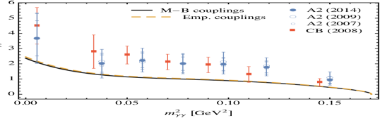
(a) $\eta\to\pi^{0}\gamma\gamma$ decay.

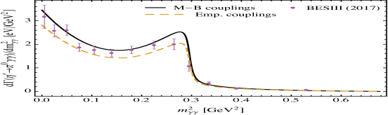
(b) $\eta^{\prime}\to\pi^{0}\gamma\gamma$ decay.

Figure 1: Comparison between the experimental diphoton energy spectra for the $\eta\to\pi^{0}\gamma\gamma$ and $\eta^{\prime}\to\pi^{0}\gamma\gamma$ and our theoretical predictions using the empirical and model-based VMD couplings. The experimental data is taken from Ref. [23] (A2), Ref. [19] (Crystal Ball) and Ref. [10] (BESIII).

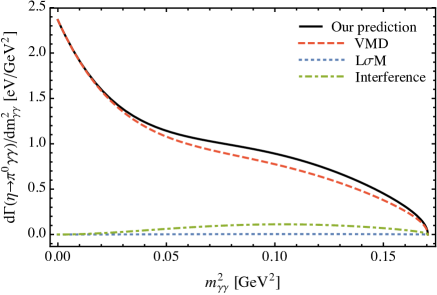
Figure 2: Contributions to the $\eta\to\pi^{0}\gamma\gamma$ diphoton energy spectrum (solid black), using the model-based VMD couplings, from intermediate vector (dashed magenta) and scalar (dashed brown) meson exchanges, and their interference (dot-dashed cyan).

Our predictions for the diphoton energy spectra are compared with the corresponding experimental data in Fig. 1. One can see from both plots that the shape of the spectra is captured well by our theoretical predictions. The spectrum of the $\eta\to\pi^{0}\gamma\gamma$ decay (Fig. 1(a)) appears to present a normalisation offset. Notwithstanding this, the exact same theoretical treatment shows very good agreement between our predictions for the $\eta^{\prime}\to\pi^{0}\gamma\gamma$ spectrum, using either set of VMD couplings, and experiment. In addition, the use of one set of couplings or the other makes little difference for the $\eta\to\pi^{0}\gamma\gamma$, though, it appears that the model-based couplings capture slightly better the experimental data for the $\eta^{\prime}\to\pi^{0}\gamma\gamma$. For this reason, as well as due to its increased aesthetic appeal and the fact that it better underpins the power of the theoretical description, from this point onwards we will stick to using the model-based VMD couplings for any subsequent calculation.

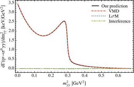
Figure 3: Contributions to the $\eta^{\prime}\to\pi^{0}\gamma\gamma$ diphoton energy spectrum (solid black), using the model-based VMD couplings, from intermediate vector (dashed magenta) and scalar (dashed brown) meson exchanges, and their interference (dot-dashed cyan).

The different contributions to the diphoton energy spectrum for the $\eta\to\pi^{0}\gamma\gamma$ decay are shown in Fig. 2. As it can be seen, the spectrum is dominated by the exchange of vector mesons, accounting for $93\%$, out of which, the weights for the $\rho^{0}$, $\omega$ and $\phi$ are $27\%$, $21\%$ and $0\%$, respectively; the remaining $52\%$ comes from the interference between the three participating vector mesons. The contribution of the scalar exchanges accounts for less than $1\%$, making it very difficult to isolate the effect of individual scalar mesons, even with the advent of more precise experimental data. The interference between the intermediate scalar and vector exchanges is constructive and accounts for about $7\%$. The contributions to the energy spectrum of the $\eta^{\prime}\to\pi^{0}\gamma\gamma$ process are displayed in Fig. 3. Once again, the exchange of vector mesons completely dominate the spectrum contributing approximately with the $100.4\%$ to the total signal, whilst the effects of scalar meson exchanges and their interference with the formers are negligible with $0\%$ and $-0.4\%$ (destructive interference), respectively. As well as this, the $\omega$ contribution prevails with the $78\%$ of the total VMD signal, whilst the $\rho^{0}$ and $\phi$ account for the $5\%$ and $0\%$, respectively; the remaining $17\%$ comes from the interference between the vector resonances.

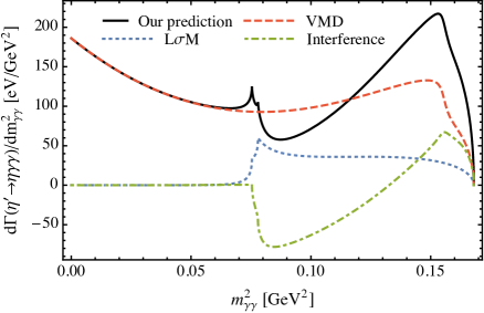
Figure 4: Contributions to the $\eta^{\prime}\to\eta\gamma\gamma$ diphoton energy spectrum (solid black), using the model-based VMD couplings, from intermediate vector (dashed magenta) and scalar (dashed brown) meson exchanges, and their interference (dot-dashed cyan).

Finally, the different contributions to the $\eta^{\prime}\to\eta\gamma\gamma$ energy spectrum are presented in Fig. 4. As expected, the contribution to the total signal from the exchange of vector mesons predominates again with about the $91\%$, with the $\rho^{0}$, $\omega$ and $\phi$ accounting for $59\%$, $15\%$ and $1\%$ of the VMD signal, respectively, and the remaining $25\%$ being the result of their interference; interestingly, the scalar meson effects turn out to be sizeable in this process, weighing approximately $16\%$, with the exchange of $\sigma$ mesons dominating the scalar signal. The interference between the scalar and vector mesons is destructive and accounts for around the $7\%$ and significantly influences the shape of the spectrum. It is worth noting the effect of using the complete one-loop propagator for the $\sigma$ exchange which manifests at the $m_{\gamma\gamma}^{2}=0.078$ GeV peak and is associated to the $\pi^{+}\pi^{-}$ threshold. This peak is absent should the Breit-Wigner propagator for the $\sigma$ exchange have been used.

Our inability to describe the total decay widths for the three $\eta^{(\prime)}\to\pi^{0}\gamma\gamma$ and $\eta^{\prime}\to\eta\gamma\gamma$ decay processes simultaneously within the same theoretical framework and values for the VMD couplings is somewhat bothersome. The offset that appears to be affecting the diphoton energy spectrum of the first process, $\eta\to\pi^{0}\gamma\gamma$ (cf. Fig. 1(a)), and consequently its integrated decay width, might be linked to a normalisation problem associated to the parameter $g$ in Eqs. (13) and (26). One could argue, though, that this parameter is fixed by the $VP\gamma$ experimental data, which is measured nowadays to a high degree of accuracy and leads to satisfactory predictions for the other two processes, i.e. $\eta^{\prime}\to\pi^{0}\gamma\gamma$ and $\eta^{\prime}\to\eta\gamma\gamma$, and, therefore, should not be changed. Despite this, an attempt has been made to assess the preferred value for the parameter $g$ by the experimental data available from Ref. [23] (A2), Ref. [19] (Crystal Ball) and Ref. [10] (BESIII) for the two $\eta^{(\prime)}\to\pi^{0}\gamma\gamma$ processes by performing a combined fit where $g$ is left as a free parameter. The resulting $g$ turns out to be roughly consistent with the one provided in Eq. (26) and used in all our calculations, which is explained by the fact that the data from BESIII contains significantly smaller uncertainties and, therefore, its statistical weight in the fit is greater. Hence, we are led to consider whether this puzzle might be somehow highlighting the need for a more sophisticated theoretical treatment; however, given the complexity associated to performing these experimental measurements and the recent history of the $\eta\to\pi^{0}\gamma\gamma$ empirical data, one cannot rule out the possibility that this decreasing trend seen over time in the measured values of the BR might persist should new and more precise measurements were available and eventually converge with our theoretical prediction, especially in light of our successful description of the data from BESIII for the other two sister processes.

VI Conclusions

In this work, we have presented a thorough theoretical analysis of the doubly radiative decays $\eta^{(\prime)}\to\pi^{0}\gamma\gamma$ and $\eta\to\eta\gamma\gamma$, and provided theoretical results for their associated decay widths and diphoton energy spectra in terms of intermediate scalar and vector meson exchange contributions using the L$\sigma$M and VMD frameworks, respectively.

A complete set of theoretical expressions for the transition amplitudes from Chiral Perturbation Theory, Vector Meson Dominance and the Linear Sigma Model have been given for the three decay processes. Some of these expressions constitute, to the best of our knowledge, the first predictions of this kind. In addition, we have provided quantitative results by making use of numerical input from the PDG [14]. In particular, for the estimation of the VMD coupling constants, $g_{V\!P\gamma}$, two different paths have been followed whereby they have been either extracted directly from the experimental $V(P)\to P(V)\gamma$ decay widths or from a phenomenological quark-based model and a fit to experimental data. A summary of the predicted decay widths, theoretical branching ratios and contributions to the total signals for the three doubly radiative decays $\eta\to\pi^{0}\gamma\gamma$ and $\eta^{\prime}\to\pi^{0}(\eta)\gamma\gamma$ is shown in Table 2, and a discussion of the results obtained and how they compare to available experimental data has been carried out. As well as this, the invariant mass spectra associated to these processes are shown in Figs. 2, 3 and 4, respectively, using the model-based VMD couplings. It is worth highlighting that, whilst vector meson exchanges vastly dominate over the scalar contributions for the $\eta^{(\prime)}\to\pi^{0}\gamma\gamma$ decays, we find that, for the $\eta^{\prime}\to\eta\gamma\gamma$, the scalar meson effects turn out to be substantial, specially that of the $\sigma$ meson, and this represents an opportunity for learning details about this still poorly understood scalar state. In particular, we look forward to the release of the energy spectrum data for the $\eta^{\prime}\to\eta\gamma\gamma$ process by the BESIII collaboration to assess the robustness of our theoretical approach.

Interestingly, our predictions for the $\eta\to\pi^{0}\gamma\gamma$ are found to be approximately a factor of two smaller than the experimental measurements, whereas our theoretical predictions for the $\eta^{\prime}\to\pi^{0}\gamma\gamma$ and $\eta^{\prime}\to\eta\gamma\gamma$ are in good agreement with recent measurements performed by BESIII. It appears that it is not possible to reconcile our predictions for the three processes with their corresponding experimental counterparts simultaneously using the same underlying theoretical framework and values for the coupling constants. This puzzle might be pointing towards potential limitations of our theoretical treatment or, perhaps, the need for more precise measurements for the $\eta\to\pi^{0}\gamma\gamma$ decay, as our approach seems to be capable of successfully predicting the experimental data for the other two processes without the need for manual adjustment of the numerical input.

As a final remark, we would very much like to encourage experimental groups to measure these decays once again to confirm whether our predictions are correct or a more refined theoretical description is required.

Appendix A Complete one-loop propagators

The complete one-loop propagators for the $\sigma$, $f_{0}$ and $a_{0}$ scalar resonances are defined as follows

$$D(s)=s-m_{R}^{2}+{\rm Re}\Pi(s)-{\rm Re}\Pi(m_{R}^{2})+i{\rm Im}\Pi(s)\ ,$$ (27)

where $m_{R}$ is the renormalised mass of the scalar meson and $\Pi(s)$ is the one-particle irreducible two-point function. ${\rm Re}\Pi(m_{R}^{2})$ is introduced to regularise the divergent behaviour of $\Pi(s)$. The propagator so defined is well behaved when a threshold is approached from below, thus, improving the usual Breit-Wigner prescription, which is not particularly suited for spinless resonances (see Ref. [38] for details).

The real and imaginary parts of $\Pi(s)$ for the $\sigma$ in the first Riemann sheet can be written as $(R(s)\equiv{\rm Re}\Pi(s),I(s)\equiv{\rm Im}\Pi(s))$

$$\qquad\qquad\qquad R(s)= \frac{g_{\sigma\pi\pi}^{2}}{16\pi^{2}}\bigg{[}2-\beta_{\pi}\log\left(\frac{1+\beta_{\pi}}{1-\beta_{\pi}}\right)\theta_{\pi}-2\bar{\beta}_{\pi}\arctan\left(\frac{1}{\bar{\beta}_{\pi}}\right)\bar{\theta}_{\pi}\bigg{]}$$ (28)

$$+\frac{g_{\sigma K\bar{K}}^{2}}{16\pi^{2}}\bigg{[}2-\beta_{K}\log\left(\frac{1+\beta_{K}}{1-\beta_{K}}\right)\theta_{K}-2\bar{\beta}_{K}\arctan\left(\frac{1}{\bar{\beta}_{K}}\right)\bar{\theta}_{K}\bigg{]}\ ,$$

$$\qquad\qquad\qquad I(s)=-\frac{g_{\sigma\pi\pi}^{2}}{16\pi}\beta_{\pi}\theta_{\pi}-\frac{g_{\sigma K\bar{K}}^{2}}{16\pi}\beta_{K}\theta_{K}\ ,$$ (29)

where $\beta_{i}=\sqrt{1-4m_{i}^{2}/s}$ for $i=(\pi,K)$, $\bar{\beta}_{i}=\sqrt{4m_{i}^{2}/s-1}$, $\theta_{i}=\theta(s-4m_{i}^{2})$, and $\bar{\theta}_{i}=\theta(4m_{i}^{2}-s)$. The couplings of the $\sigma$ to pions and kaons are written in the isospin limit; thus, $g_{\sigma\pi\pi}^{2}=\frac{3}{2}g_{\sigma\pi^{+}\pi^{-}}^{2}=\frac{3}{2}\Big{(}\frac{m_{\pi}^{2}-m_{\sigma}^{2}}{f_{\pi}}\cos{\varphi_{S}}\Big{)}^{2}$ and $g_{\sigma K\bar{K}}^{2}=2g_{\sigma K^{+}K^{-}}^{2}=\frac{1}{2}\Big{[}\frac{m_{K}^{2}-m_{\sigma}^{2}}{f_{K}}(\cos{\varphi_{S}}-\sqrt{2}\sin{\varphi_{S}})\Big{]}^{2}$. The renormalised mass of the $\sigma$ meson for the calculations is fixed to $m_{\sigma}=498$ MeV. For the $f_{0}$ exchange, the real and imaginary parts of the two-point function in the first Riemann sheet are

$$\qquad\qquad\qquad R(s)= \frac{g_{f_{0}\pi\pi}^{2}}{16\pi^{2}}\bigg{[}2-\beta_{\pi}\log\left(\frac{1+\beta_{\pi}}{1-\beta_{\pi}}\right)\theta_{\pi}-2\bar{\beta}_{\pi}\arctan\left(\frac{1}{\bar{\beta}_{\pi}}\right)\bar{\theta}_{\pi}\bigg{]}$$ (30)

$$+\frac{g_{f_{0}K\bar{K}}^{2}}{16\pi^{2}}\bigg{[}2-\beta_{K}\log\left(\frac{1+\beta_{K}}{1-\beta_{K}}\right)\theta_{K}-2\bar{\beta}_{K}\arctan\left(\frac{1}{\bar{\beta}_{K}}\right)\bar{\theta}_{K}\bigg{]}\ ,$$

$$\qquad\qquad\qquad I(s)=-\frac{g_{f_{0}\pi\pi}^{2}}{16\pi}\beta_{\pi}\theta_{\pi}-\frac{g_{f_{0}K\bar{K}}^{2}}{16\pi}\beta_{K}\theta_{K}\ ,$$ (31)

where $\beta_{i}$, $\bar{\beta}_{i}$, $\theta_{i}$ and $\bar{\theta}_{i}$ are defined as before. Once again, the couplings of the $f_{0}$ to pions and kaons are written in the isospin limit; accordingly, $g_{f_{0}\pi\pi}^{2}=\frac{3}{2}g_{f_{0}\pi^{+}\pi^{-}}^{2}=\frac{3}{2}\Big{(}\frac{m_{\pi}^{2}-m_{f_{0}}^{2}}{f_{\pi}}\sin{\varphi_{S}}\Big{)}^{2}$ and $g_{f_{0}K\bar{K}}^{2}=2g_{f_{0}K^{+}K^{-}}^{2}=\frac{1}{2}\Big{[}\frac{m_{K}^{2}-m_{f_{0}}^{2}}{f_{K}}(\sin{\varphi_{S}}+\sqrt{2}\cos{\varphi_{S}})\Big{]}^{2}$. The renormalised mass of the $f_{0}$ meson for the calculations is fixed to $m_{f_{0}}=990$ MeV. Finally, the real and imaginary parts of $\Pi(s)$ for the $a_{0}$ in the first Riemann sheet are

$$\qquad\qquad\qquad R(s)= \frac{g_{a_{0}K\bar{K}}^{2}}{16\pi^{2}}\bigg{[}2-\beta_{K}\log\left(\frac{1+\beta_{K}}{1-\beta_{K}}\right)\theta_{K}-2\bar{\beta}_{K}\arctan\left(\frac{1}{\bar{\beta}_{K}}\right)\bar{\theta}_{K}\bigg{]}$$ (32)

$$+\frac{g_{a_{0}\pi\eta}^{2}}{16\pi^{2}}\bigg{[}2-\frac{m^{2}_{\eta}-m^{2}_{\pi}}{s}\log\left(\frac{m_{\eta}}{m_{\pi}}\right)-\beta^{+}_{\pi\eta}\beta^{-}_{\pi\eta}\log\left(\frac{\beta^{-}_{\pi\eta}+\beta^{+}_{\pi\eta}}{\beta^{-}_{\pi\eta}-\beta^{+}_{\pi\eta}}\right)\theta_{\pi\eta}$$

$$-2\bar{\beta}^{+}_{\pi\eta}\beta^{-}_{\pi\eta}\arctan\left(\frac{\beta^{-}_{\pi\eta}}{\bar{\beta}^{+}_{\pi\eta}}\right)\bar{\theta}_{\pi\eta}+\bar{\beta}^{+}_{\pi\eta}\bar{\beta}^{-}_{\pi\eta}\log\left(\frac{\bar{\beta}^{+}_{\pi\eta}+\bar{\beta}^{-}_{\pi\eta}}{\bar{\beta}^{+}_{\pi\eta}-\bar{\beta}^{-}_{\pi\eta}}\right)\bar{\bar{\theta}}_{\pi\eta}\bigg{]}\ ,$$

$$\qquad\qquad\qquad I(s)=-\frac{g_{a_{0}K\bar{K}}^{2}}{16\pi}\beta_{K}\theta_{K}-\frac{g_{a_{0}\pi\eta}^{2}}{16\pi}\beta^{+}_{\pi\eta}\beta^{-}_{\pi\eta}\theta_{\pi\eta}\ ,$$ (33)

where $\beta^{\pm}_{\pi\eta}=\sqrt{1-(m_{\pi}\pm m_{\eta})^{2}/s}$, $\bar{\beta}^{\pm}_{\pi\eta}=\sqrt{(m_{\pi}\pm m_{\eta})^{2}/s-1}$, $\theta_{\pi\eta}=\theta[s-(m_{\pi}+m_{\eta})^{2}]$, $\bar{\theta}_{\pi\eta}=\theta[s-(m_{\pi}-m_{\eta})^{2}]\times\theta[(m_{\pi}+m_{\eta})^{2}-s]$, and $\bar{\bar{\theta}}_{\pi\eta}=\theta[(m_{\pi}-m_{\eta})^{2}-s]$. The couplings of the $a_{0}$ to kaons are also written in the isospin limit; hence, $g_{a_{0}K\bar{K}}^{2}=2g_{a_{0}K^{+}K^{-}}^{2}=\frac{1}{2}\Big{(}\frac{m_{K}^{2}-m_{a_{0}}^{2}}{f_{K}}\Big{)}^{2}$ and $g_{a_{0}\pi\eta}^{2}=\Big{(}\frac{m_{\eta}^{2}-m_{a_{0}}^{2}}{f_{\pi}}\cos{\varphi_{P}}\Big{)}^{2}$. For the calculations, the renormalised mass of the $a_{0}$ meson is fixed to $m_{a_{0}}=980$ MeV.

References

• [1] L. Gan, B. Kubis, E. Passemar and S. Tulin, [arXiv:2007.00664 [hep-ph]].
• [2] G. Oppo and S. Oneda, Phys. Rev.  160, 1397 (1967).
• [3] A. Baracca and A. Bramon, Nuovo Cim. A 69, 613 (1970).
• [4] L. Ametller, J. Bijnens, A. Bramon and F. Cornet, Phys. Lett. B 276, 185 (1992).
• [5] E. Oset, J. R. Pelaez and L. Roca, Phys. Rev. D 67, 073013 (2003) [hep-ph/0210282].
• [6] E. Oset, J. R. Pelaez and L. Roca, Phys. Rev. D 77, 073001 (2008) [arXiv:0801.2633 [hep-ph]].
• [7] I. Danilkin, O. Deineka and M. Vanderhaeghen, Phys. Rev. D 96, no. 11, 114018 (2017) [arXiv:1709.08595 [hep-ph]].
• [8] Y. Balytskyi, arXiv:1804.02607 [hep-ph].
• [9] Y. Balytskyi, arXiv:1811.01402 [hep-ph].
• [10] M. Ablikim et al. [BESIII Collaboration], Phys. Rev. D 96, no. 1, 012005 (2017) [arXiv:1612.05721 [hep-ex]].
• [11] M. Ablikim et al. [BESIII Collaboration], Phys. Rev. D 100, no. 5, 052015 (2019) [arXiv:1906.10346 [hep-ex]].
• [12] S. s. Fang, A. Kupsc and D. h. Wei, Chin. Phys. C 42, no. 4, 042002 (2018) [arXiv:1710.05173 [hep-ex]].
• [13] R. Escribano, Phys. Rev. D 74, 114020 (2006) [hep-ph/0606314].
• [14] M. Tanabashi et al. [Particle Data Group], Phys. Rev. D 98, 030001 (2018).
• [15] R. Escribano, PoS QNP 2012, 079 (2012) [arXiv:1207.5400 [hep-ph]].
• [16] R. Jora, Nucl. Phys. Proc. Suppl.  207-208, 224 (2010).
• [17] D. Alde et al. [Serpukhov-Brussels-Annecy(LAPP) and Soviet-CERN Collaborations], Z. Phys. C 25, 225 (1984) [Yad. Fiz.  40, 1447 (1984)].
• [18] S. Prakhov et al., Phys. Rev. C 72, 025201 (2005).
• [19] S. Prakhov, B. M. K. Nefkens, C. E. Allgower, V. Bekrenev, W. J. Briscoe, J. R. Comfort, K. Craig and D. Grosnick et al., Phys. Rev. C 78, 015206 (2008).
• [20] N. Knecht et al., Phys. Lett. B 589, 14 (2004).
• [21] L. G. Landsberg, Phys. Rept.  128, 301 (1985).
• [22] B. Di Micco et al. [KLOE Collaboration], Acta Phys. Slov.  56, 403 (2006).
• [23] B. M. K. Nefkens et al. [A2 at MAMI Collaboration], Phys. Rev. C 90, no. 2, 025206 (2014) [arXiv:1405.4904 [hep-ex]].
• [24] D. Alde et al. [Serpukhov-Brussels-Los Alamos-Annecy(LAPP) Collaboration], Z. Phys. C 36, 603 (1987).
• [25] C. Picciotto, Nuovo Cim. A 105, 27 (1992).
• [26] J. N. Ng and D. J. Peters, Phys. Rev. D 46, 5034 (1992).
• [27] P. Ko, Phys. Rev. D 47, 3933 (1993).
• [28] P. Ko, Phys. Lett. B 349, 555 (1995) [hep-ph/9503253].
• [29] A. A. Bel’kov, A. V. Lanyov and S. Scherer, J. Phys. G 22, 1383 (1996) [hep-ph/9506406].
• [30] S. Bellucci and C. Bruno, Nucl. Phys. B 452, 626 (1995) [hep-ph/9502243].
• [31] J. Bijnens, A. Fayyazuddin and J. Prades, Phys. Lett. B 379, 209 (1996) [hep-ph/9512374].
• [32] J. N. Ng and D. J. Peters, Phys. Rev. D 47, 4939 (1993).
• [33] Y. Nemoto, M. Oka and M. Takizawa, Phys. Rev. D 54, 6777 (1996) [hep-ph/9602253].
• [34] A. Bramon, R. Escribano and M. D. Scadron, Phys. Lett. B 403 (1997), 339-343 [arXiv:hep-ph/9703313 [hep-ph]].
• [35] A. Bramon, R. Escribano and M. Scadron, Phys. Lett. B 503 (2001), 271-276 [arXiv:hep-ph/0012049 [hep-ph]].
• [36] R. Escribano and E. Royo, Phys. Lett. B 807 (2020), 135534 [arXiv:2003.08379 [hep-ph]].
• [37] S. Gonzàlez-Solís and E. Passemar, Eur. Phys. J. C 78, no. 9, 758 (2018) [arXiv:1807.04313 [hep-ph]].
• [38] R. Escribano, A. Gallegos, J. L. Lucio M, G. Moreno and J. Pestieau, Eur. Phys. J. C 28, 107 (2003) [arXiv:hep-ph/0204338].
• [39] T. Bhattacharya and S. Willenbrock, Phys. Rev. D 47 (1993), 4022-4027.