A Pontryaghin maximum principle approach for the optimization of dividends/consumption of spectrally negative Markov processes, until a generalized draw-down time

Abstract.

The first motivation of our paper is to explore further the idea that, in risk control problems, it may be profitable to base decisions both on the position of the underlying process $X_{t}$ and on its supremum $\overline{X}_{t}:=\sup_{0\leq s\leq t}X_{s}$. Strongly connected to Azema-Yor/generalized draw-down/trailing stop time (see [AY79]), this framework provides a natural unification of draw-down and classic first passage times.

We illustrate here the potential of this unified framework by solving a variation of the De Finetti problem of maximizing expected discounted cumulative dividends/consumption gained under a barrier policy, until an optimally chosen Azema-Yor time, with a general spectrally negative Markov model.

While previously studied cases of this problem [APP07, SLG84, AS98, AVZ17, AH18, WZ18] assumed either Lévy or diffusion  models, and the draw-down function to be fixed, we describe, for a general spectrally negative Markov model, not only the optimal barrier but also the optimal draw-down function. This is achieved by solving a variational problem tackled by Pontryaghin’s maximum principle. As a by-product we show that in the Lévy case the classic first passage solution is indeed optimal; in the diffusion case, we obtain the optimality equations, but the existence of solutions improving the classic ones is left for future work.

Keywords: first passage, draw-down process, spectrally negative process, scale functions, dividends, dividends barrier optimization, de Finetti, optimal harvesting, variational problem

1. A brief review of the classic spectrally negative first passage theory

Control of dividends/optimal consumption and capital injections. Many control problems in risk theory concern versions of $X_{t}$ which are reflected/constrained/regulated at first passage times (below or above):

(1) $$X_{t}^{[a}=X_{t}+\;L_{t},\quad X^{b]}_{t}=X_{t}-U_{t}.$$

Here,

$$L_{t}=L^{[a}_{t}=-(\underline{X}_{t}-a)_{-},\quad\underline{X}_{t}=\inf_{0\leq t^{\prime}\leq t}X_{t^{\prime}},$$

$$U_{t}=U^{b]}_{t}=\left(\overline{X}_{t}-b\right)_{+},\quad\overline{X}_{t}:=\sup_{0\leq t^{\prime}\leq t}X_{t^{\prime}},$$

are the minimal ’Skorohod regulators’ constraining $X_{t}$ to be larger than $a$, and smaller than $b$, respectively, and we use the notation $x_{+}=\max(x,0)$ and $x_{-}=\min(x,0)$.

Financial management and other applications require also studying the running maximum and the process reflected at its maximum/drawdown

$$Y_{t}=\overline{X}_{t}-X_{t},\quad\overline{X}_{t}=\sup_{0\leq t^{\prime}\leq t}X_{s},$$

as well as the running infimum and the process reflected from below/drawup

$$\underline{Y}_{t}=X_{t}-\underline{X}_{t},\quad\underline{X}_{t}=\inf_{0\leq t^{\prime}\leq t}X_{s}.$$

The first passage times of the reflected processes, called draw-down/regret time and draw-up time, respectively, are defined for $d>0$ by

(2) $$\tau_{d} :=\inf\{t\geq 0:\overline{X}(t)-X(t)\geq d\},$$

$$\underline{\tau}_{d} :=\inf\{t\geq 0:X(t)-\underline{X}(t)\geq d\}.$$

Such times turn out to be optimal in several stopping problems, in statistics [Pag54] in mathematical finance/risk theory and in queueing. More specifically, they figure in risk theory problems involving dividends at a fixed barrier or capital injections, and in studying idle times until a buffer reaches capacity in queueing theory– see for example [Tay75, Leh77, SS93, AKP04, MP12, SXZ08, Car14, LLZ17a, LLZ17b]– for results and references to numerous applications of draw-downs and draw-ups.

Optimization of dividends. One important optimization problem, going back to Bruno de Finetti [dF57], is to estimate the maximal expected discounted cumulative dividends of a financial company until its ruin.

Solving this is nontrivial even for Lévy process without positive jumps (a “multi-band” continuation region may be necessary); therefore, given the usual data uncertainty inherent to real problems, it is reasonable to restrict to simpler dividends policies which distribute all surpluses above a fixed level $b$, called dividends barrier. For fixed $b$, we arrive then to the optimal dividends barrier problem with ruin stopping.

Note that the time of ruin of the “Skorohod regulated process” $X^{b]}_{t}=X_{t}-U_{t}$ may be decomposed as:

(3) $$T_{0}^{b]}:=T_{0,-}\;{\mathbf{1}}_{T_{0,-}<T_{b,+}}+\tau_{b}\;{\mathbf{1}}_{T_{b,+}<T_{0,-}}.$$

The “de Finetti barrier problem” consists in maximizing over $b$ the present value of all dividend payments at the barrier $b$, until the time $T_{0}^{b]}$:

(4) $$V^{b}(x)=V_{q}^{b}(x):=E_{x}\left[\int_{0}^{T_{0}^{b]}}e^{-qt}d(\overline{X}_{t}-b)_{+}\right].$$

In the case of a spectrally negative Lévy process $X_{t}$, the value function (4) and many other results may be expressed in terms of the scale function $W_{q}$ [Ber98, Kyp14]. In preparation for the spectrally negative Markov case, we will also express the value function in terms of the logarithmic derivative

(5) $$\nu_{q}(x):=\frac{W_{q}^{\prime}(x+)}{W_{q}(x)}$$

since it became apparent in [LLZ17b, ALL18] that for spectrally negative Markov processes  it is more convenient to introduce first a natural extension $\nu_{q}(x,y)$ (defined via the limit (12)) of the logarithmic derivative than the corresponding extension $W_{q}(x,y)$.

The Lévy factorization of the “gambler’s winning/survival” probability may also be written as

(6) $$E_{x}\left[e^{-qT_{b,+}}1_{\left\{T_{b,+}<T_{a,-}\right\}}\right]=\frac{W_{q}(x-a)}{W_{q}(b-a)}=e^{-\int_{x}^{b}\nu_{q}(s-a)ds}.$$

Applying now the strong Markov property  in (4) yields

$$V^{b}(x)=E_{x}\left[e^{-qT_{b,+}};T_{b,+}<T_{0,-}\right]E_{b}\left[\int_{0}^{T_{0}^{b]}}e^{-qt}d(\overline{X}_{t}-b)\right]$$

(7) $$=\frac{W_{q}(x)}{W_{q}(b)}V^{b}(b)=\frac{W_{q}(x)}{W_{q}(b)}\frac{W_{q}(b)}{W_{q}^{\prime}(b)}=e^{-\int_{x}^{b}\nu_{q}(m)dm}\frac{1}{\nu_{q}(b)},$$

where we have used (6) and

$$V^{b}(b)=\frac{1}{\nu_{q}(b)}$$

cf. [Ber98, KP07, AI18]. To understand the last equality, note that the dividends starting from $b$ equal the local time spent at the reflecting boundary $b$, and that the latter has an exponential law, the rate of which is $\nu_{q}(b)$, since the function $\nu_{q}(x)$ is the rate of downwards excursions strictly larger than $x$, and occurring before an exponential horizon of rate $q$ [Ber98, Don05].

We will make use below of the fact that $\nu_{q}(x)$ is nonincreasing and that

(8) $$\nu_{q}(x)\geq\Phi_{q}$$

where $\Phi_{q}$ is the unique positive root of the Cramér-Lundberg equation [Ber98, Kyp14]

(9) $$\kappa(s):=Log\Big{(}E_{0}[e^{sX_{1}}]\Big{)}=q.$$

Assumption 1.

To be able to write below equations like $\nu_{q}(x)=\frac{W_{q}^{\prime}(x)}{W_{q}(x)}$ and formulas like (39) we will assume throughout the paper that $W_{q}(x)$ is three times differentiable in the Lévy case. In the spectrally negative Markov case, we will assume the scale function $W_{q}(x,y)$ (see last section) to be three times differentiable in $x$, or, alternatively, $\nu_{q}(x,y):=\frac{\frac{\partial W_{q}(x,y)}{\partial x}}{W_{q}(x,y)}$ will be assumed to be twice differentiable.

See [CKS11] for more information on the smoothness of scale functions for Lévy processes, and note this problem has not yet been studied for spectrally negative Markov processes.

In conclusion, the Lévy De-Finetti barrier objective has a simple expression in terms of either the $W_{q}$ scale function or of $\nu_{q}$:

(10) $$V^{b}(x)=\begin{cases}\frac{W_{q}(x)}{W_{q}^{\prime}(b)}=e^{-\int_{x}^{b}\nu_{q}(m)dm}\frac{1}{\nu_{q}(b)},&x\leq b,\\ V^{b}(x)=x-b+V^{b}(b),&x>b\end{cases}.$$

where the second line follows upon completing the barrier strategy by ”reduce holdings to $b$ when above”.

Maximizing over the reflecting barrier $b$ is simply achieved by finding the roots of

(11) $$W_{q}^{\prime\prime}(b^{*})=0\Leftrightarrow\frac{\partial}{\partial b}\Big{[}\frac{1}{\nu_{q}(b^{*})}\Big{]}=1.$$

This is a smooth fit equation at $b^{*}$ (see (10)).

Our paper replaces ruin in the de Finetti dividends barrier optimization by more general Azema-Yor /generalized draw-down stopping times, to be chosen optimally. Then, the appropriate tool is the calculus of variations/optimal control. Let us note a recent related paper using general draw-down stopping times [WZ18], who study optimality of barrier policies under a fixed prespecified draw-down function.

First passage theory for spectrally negative Markov processes. Prior to [LLZ17b], the classic and draw-down first passage literatures were restricted mostly to parallel analytic treatments of the two particular cases of diffusions and of spectrally negative Lévy processes. [LLZ17b] showed that a direct unified approach (inspired by [Leh77] in the case of diffusions) may achieve the same results for all time homogeneous Markov processes; the known results for diffusions and spectrally negative Lévy processes are just particular cases of general formulas, once expressed in terms of $W,Z$, or of the differential exit parameters $\nu,\delta$ – see below.

Assume the existence of differential versions of the ruin and survival problems:

Assumption 2.

For all $q,\theta\geq 0$ and $u\leq x$ fixed, assume that $\overline{\Psi}_{q}^{b}(x,a)$ and $\Psi_{q,\theta}^{b}(x,a)$ are differentiable in $b$ at $b=x$, and in particular that the following limits exist:

(12) $$\nu_{q}(x,a):=\lim_{\varepsilon\downarrow 0}\frac{1-\overline{\Psi}_{q}^{x+\varepsilon}(x,a)}{\varepsilon}\;\bf{(total\;infinitesimal\;hazard\;rate)}$$

and

(13) $${\delta}_{q,\theta}(x,a):=\lim_{\varepsilon\downarrow 0}\frac{\Psi_{q,\theta}^{x+\varepsilon}(x,a)}{\varepsilon}\;\bf{(infinitesimal\;spatial\,killing\;rate)}.$$

Remark 1.

It turns out that everything reduces to the differentiability of the two-sided ruin and survival probabilities as functions of the upper limit. Informally, we may say that the pillar of first passage theory for spectrally negative Markov processes is proving the existence of $\nu,\delta$. Later, the differential characteristics $\nu$, $\delta$ were extended in [ALL18] to the case of generalized draw-down times, which unify classic first passage times and draw-down times.

Since results for spectrally negative Lévy processes  (like the de Finetti problem  considered here) require often not much more than the strong Markov property, it was natural to attempt to extend them to the spectrally negative strong Markov case. As expected, everything worked out almost smoothly for “Lévy -type cases” like random walks [AV17], Markov additive processes [IP12], and Lévy processes with $\Omega$ state dependent killing [IP12].

However, diffusions and spectrally negative Lévy processes were always tackled by different methods until the pioneering work [LLZ17b], who showed that certain draw-down problems could be treated by a unified approach, inspired by [Leh77] in the case of diffusions, which can be extended to all time homogeneous Markov processes.

When switching to spectrally negative Markov processes,  $W_{q}(x)$ must be replaced by a two variables function $W_{q}(x,y)$ (which reduces in the Lévy case to $W_{q}(x,y)=\widetilde{W}_{q}(x-y)$, with $\widetilde{W}_{q}$ being the scale function of the Lévy process).

However, the existence of $W$, as well as that of the scale function $Z$, are not obvious in the non-Lévy case, and it becomes more convenient to replace them by differential versions $\nu$ and $\delta$ defined by(13), (13) below.

Computing $\nu,\delta,W,Z$ is still an open problem, even for simple classic processes like the Ornstein-Uhlenbeck and the Feller branching diffusion with jumps. However, one may cut through this Gordian node by restricting to processes for which the limits defining $\nu,\delta$ exist, and leaving to the user the responsibility to check this for their process. With this caveat, the results of [LLZ17b, ALL18] provide a unifying umbrella for spectrally negative Lévy processes, diffusions, branching processes(including with immigration), logistic branching processes, etc. Surprisingly, all these processes which were traditionally studied separately, may be viewed as particular cases of a unified general first passage theory for spectrally negative strong Markov processes!

In this paper we illustrate the potential of this framework via one application, a variation of the de Finetti problem of maximizing expected discounted cumulative dividends, where we replace stopping at ruin by an optimally chosen Azema-Yor/generalized draw-down stopping time.

Contents. We start by reviewing in Section 1 the classic spectrally negative first passage theory, and in Section 2 the first passage theory with generalized draw-down /Azema-Yor stopping times. Section 3 introduces the de Finetti dividends optimization problem with generalized draw-down /Azema-Yor stopping times for spectrally negative Markov processes. Section 4 spells out the calculus of variations problem to be solved, and Section 5 offers its solution via a Pontryaghin-type approach.

Section 6 presents a detailed analysis of the particular case of Lévy processes. Finally, Section 7 considers a more general class of diffusions (general functions of drifted Brownian motion with particular emphasis on logarithmic cases).

2. Generalized draw-down stopping for processes without positive jumps

Generalized draw-down times appear naturally in the Azema-Yor solution of the Skorokhod embedding problem [AY79], and in the Dubbins-Shepp-Shiryaev, Peskir and Hobson optimal stopping problems [DSS94, Pes98, Hob07]. Importantly, they allow a unified treatment of classic first passage and draw-down times (see also [ALL18] for a further generalization to taxed processes)–see [AVZ17, LVZ17]. The idea is to replace the upper side of the rectangle by a parametrized curve

$$(x,y)=({\widehat{d}}(s),d(s)),\quad{\widehat{d}}(s)=s-d(s),$$

where $s=x+y$ represents the value of $\overline{X}_{t}$ during the excursion which intersects the upper boundary at $(x,y)$. See Figure 1, where we put ${\widehat{d}}(s):=s-d(s)$.

Alternatively, parametrizing by $x$ yields $y=h(x),h(x)=(l)^{-1}(x)-x$ (note $Y_{t}\geq d(\overline{X}_{t})\Leftrightarrow Y_{t}\geq h(X_{t})$).

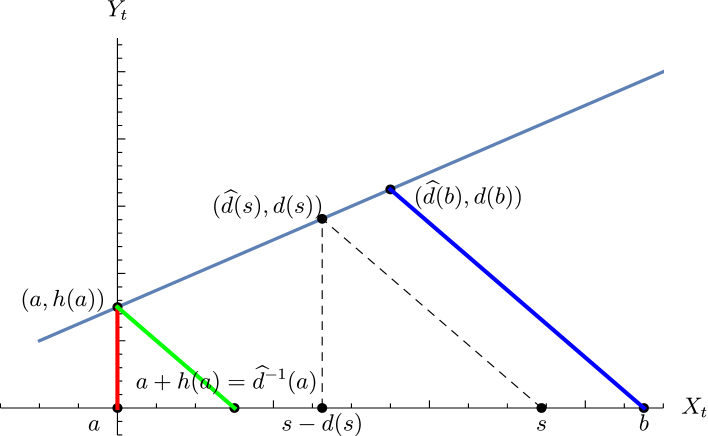
Figure 1.    Exit of $(X,Y)$ from a trapezoid with $a=0$, $d(x)=(1-\xi)x+d=\frac{1}{3}x+1$

Definition 2.

[AY79, LVZ17] For any function $d(s)>0$ such that ${\widehat{d}}(s)=s-d(s)$ is nondecreasing, a generalized draw-down time is defined by

(14) $$\tau_{d}:=\inf\{t\geq 0:Y_{t}>d(\overline{X}_{t})\}=\inf\left\{t\geq 0:X_{t}<{\widehat{d}}(\overline{X}_{t})\right\}.$$

Introduce

$$\widetilde{Y}_{t}:=Y_{t}-d(\overline{X}_{t}),\;{t\geq 0}$$

to be called draw-down type process. Note that we have $\widetilde{Y}_{0}=-{\widehat{d}}(X_{0})<0$, and that the process $\widetilde{Y}_{t}$ is in general non-Markovian. However, it is Markovian during each negative excursion of $X_{t}$, along one of the oblique lines in the geometric decomposition sketched in Figure 1.

Example 3.

With affine functions

(15) $$d(x)=(1-\xi)x+d\Leftrightarrow{\widehat{d}}(x)=\xi x-d,\xi\in{[0,1]}$$

$$\Leftrightarrow h(x)=\frac{(1-\xi)x+d}{\xi},\,\xi\in[0,1],d\geq 0,$$

we obtain the affine draw-down/regret times studied in [AVZ17].

Affine draw-down times reduce to a classic draw-down time (2) when $\xi=1,d(x)=d$, and to a ruin time when $\xi=0,{\widehat{d}}(x)=-d,d(x)=x+d$. When $\xi$ varies, we are dealing with the pencil of lines passing through $(x,y)=(-d,d)$. In particular, for $\xi=1$ we obtain an infinite strip, and for $\xi=0,d=0,$ we obtain the positive quadrant (this case corresponds to the classic ruin time).

One of the merits of affine draw-down times is that they allow unifying the classic first passage theory with the draw-down theory [AVZ17]. A second merit is that they intervene in the variational problem considered below.

3. Optimal dividends barrier problem for spectrally negative Markov processes with generalized draw-down stopping

Consider now the extension of de Finetti’s optimal dividend problem

(16) $$V^{b}(x)=V_{q,{\widehat{d}}(.)}^{b}(x):=E_{x}\left[\int_{0}^{\tau^{b]}_{d}}e^{-qt}\mathrm{d}(\overline{X}_{t}-b)\right],$$

where $\tau^{b]}_{d}$ denotes a generalized draw-down time for the process $X_{t}^{b]}$ reflected at $b$. Note that $V^{b}$ depends now also on the “spatial killing function” ${\widehat{d}}(.)$.

Remark 4.

This definition assumes that the initial point satisfies $X_{0}=\overline{X}_{0}=x$, i.e. that the starting point is on the $x$ axis in figure 1.

The strong Markov property  yields again an explicit decomposition formula

(17) $$V^{b}(x)=E_{x}\left[e^{-qT_{b,+}}1_{\left\{T_{b,+}<\tau^{b]}_{d}\right\}}\right]V^{b}(b).$$

Furthermore, by [ALL18, Thm1] it holds that

(18) $$E_{x}\left[e^{-qT_{b,+}}1_{\left\{T_{b,+}<\tau^{b]}_{d}\right\}}\right]=e^{-\int_{x}^{b}\nu_{q}(z,{\widehat{d}}(z))\mathrm{d}z},$$

where $\nu_{q}(x,{\widehat{d}}(x))$ is defined in (12).

Concerning the expectation of the dividends starting from the barrier $v(b)=V^{b}(b)$, one may show again via standard bounding arguments (see for example [CKLP18, Sec 4]) that

(19) $$v(b)=v_{q}(b,{\widehat{d}}(b)):=E_{b}\left[\int_{0}^{T_{d}}e^{-qt}\mathrm{d}(\overline{X}_{t}-b)\right]=\nu_{q}(b,{\widehat{d}}(b))^{-1}.$$

Note that in the Lévy case, using $x-{\widehat{d}}(x)=d(x)$, the equations above simplify to:

$$V^{b}(x)=\frac{W_{q}(d(x))}{W_{q}(d(b))}\nu_{q}(d(b))^{-1},$$

which checks with [WZ18, Lem. 3.1-3.2].

4. A variational problem for de Finetti’s optimal dividends until a generalized draw-down time, with a bound on the initial and total draw-down/regret area

Let us consider now de Finetti’s optimal dividends with draw-down stopping. Suppose $X_{0}=\overline{X}_{0}=a\geq 0$, and view the total trapezoidal area $A(b)=\int_{a}^{b}\sqrt{2}d(s)\mathrm{d}s$ between the green and blue lines, in which the bivariate process $(X_{t},Y_{t})$ is allowed to evolve, as a measure of risk. With no upper bounds on $A(b)$, the optimum will be $b=\infty$. We set therefore an upper limit $A(b)\leq K\sqrt{2}$, and also an upper limit $d_{0}=d(a)$ on the initial maximum regret. Using (17)-(19), we arrive to the following Bolza problem

(20) $$\begin{cases}\max_{d(y)\geq 0,\ {d(y),y-d(y)\text{ nondecreasing}}}V^{b}(a)=\max_{d(y)\geq 0,{d(y),y-d(y)\text{ nondecreasing}}}\frac{e^{-\int_{a}^{b}\nu_{q}(y,{\widehat{d}}(y))\mathrm{d}y}}{\nu_{q}(b,{\widehat{d}}(b))}\\ A(b)\leq K\sqrt{2}\\ b,d(b)\text{ free},d(a)\leq d_{0}\end{cases}$$

After taking logarithms, (20) becomes:

(21) $$\begin{cases}\min_{d(y)\geq 0,{d(y),y-d(y)\text{ nondecreasing}}}\int_{a}^{b}\nu_{q}(y,{\widehat{d}}(y))\mathrm{d}y+\log({\nu_{q}(b,{\widehat{d}}(b))}=\\ \min_{d(y)\geq 0,{d(y),y-d(y)\text{ nondecreasing}}}\int_{a}^{b}\Big{(}\nu_{q}(y,{\widehat{d}}(y))+\frac{\nu_{q}^{\prime}(y,{\widehat{d}}(y))}{\nu_{q}(y,{\widehat{d}}(y))}\Big{)}\mathrm{d}y+\log({\nu_{q}(a,{\widehat{d}}(a))}\\ \int_{a}^{b}d(y)dy\leq K\\ b,d(b)\text{ free},d(a)\leq d_{0}.\end{cases}$$

Remark 5.

Let us relate (21) to the classic de Finetti problem, which is the particular case obtained by imposing the additional constraint ${\widehat{d}}(y)={\widehat{d}}(a)\Leftrightarrow d(y)=d(a)+y-a\Longrightarrow X_{t}\geq{\widehat{d}}(a),\forall t$. Here the constraint $d(a)=d_{0}\Leftrightarrow{\widehat{d}}(a)=a-d_{0}$ quantifies an imposed initial bankruptcy level, and the subsequent values $d(y)$ quantify bankruptcy levels dependent on the attained maximum $y$. The area constraint is thus an acceptable ”integrated bankruptcy risk”.

Remark 6.

If we fix the draw-down boundary in (21), the optimality condition for the dividend barrier $b^{*}$ is

(22) $$\nu_{q}(b^{*},{\widehat{d}}(b^{*}))+\frac{\nu_{q}^{\prime}(b^{*},{\widehat{d}}(b^{*}))}{\nu_{q}(b^{*},{\widehat{d}}(b^{*}))}=0,$$

which implies the classic smooth-fit equation (11). In the Lévy case, the optimal draw-down boundary turns out to be De Finetti’s ${\widehat{d}}(y)=const$, and thus the smooth-fit equation at $b^{*}$ determines completely the solution.

5. Solving the de Finetti Markovian variational problem by Pontryaghin’s minimum principle

As usual in modern calculus of variations, we let $u(t)$ denote the derivative of $d(t)$, and reformulate the problem as

(23) $$\left\{\begin{split}&V(a,d(a)):=\inf_{u}J_{b}(a,d,u),\\ &where\\ &J_{b}(a,d,u):=\left.\begin{split}&\int_{{a}}^{b}\left(\nu_{q}\left(t,t-d(t,u)\right)+\frac{\partial_{1}\nu_{q}\left(t,t-d(t,u)\right)+\partial_{2}\nu_{q}\left(t,t-d(t,u)\right)(1-u(t))}{\nu_{q}\left(t,t-d(t,u)\right)}\right)dt\\ &{+\log\left(\nu_{q}\left(a,a-d(a)\right)\right)}\end{split}\right.\\ &s.t.\ \int_{{a}}^{b}d(t,u)dt\leq K,\\ &\partial_{t}d(t,u)=u(t),\ d(a,u)=d(a)\in[0,d_{0}]\\ &u\textnormal{ measurable },u\in\left[u_{*}=0,u^{*}=1\right].\end{split}\right.$$

Remark 7.

In the case of non-decreasing draw-down functions, requiring $d(t)\geq 0$ amounts to imposing the initial condition $d(a)\geq 0$. In absence of such assumptions, one deals with state constraints and Pontryagin’s principle has a (slightly) different form

This is the first step towards defining an associated Hamiltonian $H(t,d,u,p)$ (24), where the costate $p(t)$ satisfies the conjugate equation (25). Then, one may apply Pontryagin’s maximum principle [Pon18].

It is convenient here to break the solution in four cases, with free area constraint

$$\int_{{a}}^{b^{*}}d^{opt}(t)dt=(resp.<)K,$$

respectively with free starting data $d(a)>0$ and with fixed starting data $d(a)=0$.

5.1. Optimality Without Area Constraints

5.1.1. Arguments for Free Initial $d(a)>0$

The associated Hamiltonian to be minimized is

(24) $$\begin{split}H(t,d,u,p):=&pu+\left(\nu_{q}\left(t,t-d\right)+\frac{\partial_{1}\nu_{q}\left(t,t-d\right)+\partial_{2}\nu_{q}\left(t,t-d\right)(1-u)}{\nu_{q}\left(t,t-d\right)}\right)\\ =&\nu_{q}\left(t,t-d\right)+\frac{\partial_{1}\nu_{q}\left(t,t-d\right)+\partial_{2}\nu_{q}\left(t,t-d\right)}{\nu_{q}\left(t,t-d\right)}+\left(p-\frac{\partial_{2}\nu_{q}\left(t,t-d\right)}{\nu_{q}\left(t,t-d\right)}\right)u,\end{split}$$

with costate $p(t)$ satisfying:

(25) $$\begin{split}\partial_{t}p(t)=&{-\partial_{d}H(t,d^{opt},u^{opt},p)}\\ =&\partial_{2}\left(\nu_{q}+\frac{\partial_{1}\nu_{q}+\partial_{2}\nu_{q}}{\nu_{q}}\right)\left(t,t-d^{opt}(t)\right)-\partial_{2}\Big{[}\frac{\partial_{2}\nu_{q}}{\nu_{q}}\Big{]}\left(t,t-d^{opt}(t)\right)u^{opt}(t).\end{split}$$

Remark 8.

Note that due to linearity in $u$, optimizing the Hamiltonian $H(t,d,u,p)$ yields optimal control policies $u^{opt}$ of bang-bang type, except on sets where $p(t)=\frac{\partial_{2}\nu_{q}\left(t,t-d(t)\right)}{\nu_{q}\left(t,t-d(t)\right)}$.

The previous remark implies:

Lemma 9.

The optimal draw-down function $d$ may have three possible types of subintervals.

1. On sets $\left[\alpha_{1},\beta_{1}\right]$ on which $u^{opt}=u_{*}=0$, it follows from (23) that $d^{opt}(t)=d(\alpha_{1})$ is constant. On such sets, (25) yields

   (26) $$p(t)=p(\alpha_{1})+\int_{\alpha_{1}}^{t}\partial_{2}\left(\nu_{q}+\frac{\partial_{1}\nu_{q}+\partial_{2}\nu_{q}}{\nu_{q}}\right)\left(s,s-d\left(\alpha_{1}\right)\right)ds>\frac{\partial_{2}\nu_{q}\left(t,t-d\left(\alpha_{1}\right)\right)}{\nu_{q}\left(t,t-d\left(\alpha_{1}\right)\right)},$$

   for all $t\in\left(\alpha_{1},\beta_{1}\right)$ by noting that the coefficient of $u$ in $H$ should be positive. We either have $\alpha_{1}=a$ or equality at $t=\alpha_{1}$ in (26). Similar assertions hold true at $t=\beta_{1}$.

2. Sets $\left[\alpha_{2},\beta_{2}\right]$ on which the costate satisfies the structural equality $p(t)=\frac{\partial_{2}\nu_{q}\left(t,t-d(t)\right)}{\nu_{q}\left(t,t-d(t)\right)}.$ Recalling that $\partial_{t}d(t)=u(t)$ and combining with (25), whenever the function $\nu_{q}$ is regular enough (of class $C^{2}$ such that second-order mixed partial derivatives coincide), this leads to the following implicit “structural equation” satisfied by the optimal draw-down $d^{opt}$:

   (27) $$\partial_{2}\nu_{q}\left(t,t-d^{opt}(t)\right)=0.$$

3. The third and last case to be taken into consideration leads to $u^{opt}=u^{*}=1$. On sets $\left(\alpha_{3},\beta_{3}\right)$ corresponding to this case (note that here it holds that that $t-d(t)=\alpha_{3}-d\left(\alpha_{3}\right)$), one gets

   (28) $$\left\{\begin{split}d(t)&=d(\alpha_{3})+\left(t-\alpha_{3}\right),\\ p(t)&=p\left(\alpha_{3}\right)+\int_{\alpha_{3}}^{t}\partial_{2}\nu_{q}\left(s,\alpha_{3}-d\left(\alpha_{3}\right)\right)ds+\frac{\partial_{2}\nu_{q}}{\nu_{q}}\left(t,\alpha_{3}-d\left(\alpha_{3}\right)\right)-{\frac{\partial_{2}\nu_{q}}{\nu_{q}}\left(\alpha_{3},\alpha_{3}-d\left(\alpha_{3}\right)\right)}\\ &\leq\frac{\partial_{2}\nu_{q}\left(t,\alpha_{3}-d\left(\alpha_{3}\right)\right)}{\nu_{q}\left(t,\alpha_{3}-d\left(\alpha_{3}\right)\right)}\end{split}\right.$$

Remark 10.

One should add the following transversality conditions, taking into account the liberty to choose $b$ and $d(b)$, and the initial conditions $d(a)$:

1. The first condition is linked to the freedom of $b$

   (29) $$H(b^{*})=0.$$

2. The second condition is linked to the freedom of $d(b)$

   (30) $$p(b^{*})=0.$$

3. If the initial position $d(a)$ is not fixed (thus, one searches for $0<d(a)<d_{0}$), one further imposes

   (31) $${p(a)=\frac{\partial_{2}\nu_{q}}{\nu_{q}}\left(a,a-d(a)\right)}.\\$$

   In other words, assuming optimality, either the optimal initial position satisfies $0<d(a)<d_{0}$ and, in such cases, (31) holds true, or, otherwise, $d(a)\in\left\{0,d_{0}\right\}$ (saturating this constraint for some a priori given $d_{0}$).

5.1.2. Arguments for Null Initial Datum $d(a)=0$

The program presented before still holds true but having fixed the initial datum $d(a)=0$, the transversality conditions are reduced to (29, 30).

5.2. Optimality With Area Constraints

Again, as before, we reason for $d(a)>0$ (the restriction $d(a)=0$ being taken into account by the absence of the transversality condition (31).

To cope with the additional constraint $\int_{{a}}^{b^{*}}d(y)dy{\leq}K$, we use a classic trick and introduce a further variable in the control system. We deal now with

(32) $$\left\{\begin{split}&V(a,d(a),e(a)):=\inf_{u}J_{b}^{{+}}(a,d,e,u),\\ where\ &J_{b}^{{+}}(a,d,e,u):=J_{b}(a,d,u),\\ s.t.&\ \partial_{t}d(t,u)=u(t),\partial_{t}e(t,u)=d(t,u),\ e(a,u)=e(a),\ d(a,u)=d(a),\ e(b,u)=K.\\ &u\in\left[0,1\right].\end{split}\right.$$

The associated Hamiltonian is

(33) $$\begin{split}H&{}^{+}(t,d,e,u,p,r):=H(t,d,u,p)+rd\\ &=\nu_{q}\left(t,t-d\right)+\frac{\partial_{1}\nu_{q}\left(t,t-d\right)+\partial_{2}\nu_{q}\left(t,t-d\right)}{\nu_{q}\left(t,t-d\right)}+\left(p-\frac{\partial_{2}\nu_{q}\left(t,t-d\right)}{\nu_{q}\left(t,t-d\right)}\right)u+rd.\end{split}$$

The arguments are exactly the same but the equations of the costates are given here by

(34) $$\left\{\begin{split}\partial_{t}&r(t)=\left(-\partial_{e}H^{+}(t,d,e,u,p,r)\right)=0{\Longrightarrow r(t)=r=const}\\ \partial_{t}&p(t)=\left(-\partial_{d}H^{+}(t,d^{opt},e^{opt},u^{opt},p,r)=\right)-\partial_{d}H(t,d^{opt},u^{opt},p)-r\\ &=\partial_{2}\left(\nu_{q}+\frac{\partial_{1}\nu_{q}+\partial_{2}\nu_{q}}{\nu_{q}}\right)\left(t,t-d^{opt}(t)\right)+\frac{\left(\partial_{2}\nu_{q}\right)^{2}-\partial_{22}^{2}\nu_{q}\times\nu_{q}}{\nu_{q}^{2}}\left(t,t-d^{opt}(t)\right)u^{opt}(t)-r.\end{split}\right.$$

Cases are exactly the same as before. Formulas (26) and (28) are similar:

(35) $$p(t)=p(\alpha_{1})+\int_{\alpha_{1}}^{t}\partial_{2}\left(\nu_{q}+\frac{\partial_{1}\nu_{q}+\partial_{2}\nu_{q}}{\nu_{q}}\right)\left(s,s-d\left(\alpha_{1}\right)\right)ds-r\left(t-\alpha_{1}\right)>\frac{\partial_{2}\nu_{q}\left(t,t-d\left(\alpha_{1}\right)\right)}{\nu_{q}\left(t,t-d\left(\alpha_{1}\right)\right)},$$

resp.

(36) $$\left\{\begin{split}d(t)&=d(\alpha_{3})+\left(t-\alpha_{3}\right),\\ p(t)&=p\left(\alpha_{3}\right)+\int_{\alpha_{3}}^{t}\partial_{2}\left(\nu_{q}\left(s,\alpha_{3}-d\left(\alpha_{3}\right)\right)\right)ds+\frac{\partial_{2}\nu_{q}}{\nu_{q}}\left(t,\alpha_{3}-d\left(\alpha_{3}\right)\right)\\ &-{\frac{\partial_{2}\nu_{q}}{\nu_{q}}\left(\alpha_{3},\alpha_{3}-d\left(\alpha_{3}\right)\right)-r\left(t-\alpha_{3}\right)}\\ &\leq\frac{\partial_{2}\nu_{q}\left(t,\alpha_{3}-d\left(\alpha_{3}\right)\right)}{\nu_{q}\left(t,\alpha_{3}-d\left(\alpha_{3}\right)\right)}\end{split}\right.$$

Finally, the structure equation (27) becomes

(37) $${\partial_{2}\nu_{q}\left(t,t-d^{opt}(t)\right)=r.}$$

The transversality conditions (see Remark 13) are similar and allow to determine the optimal horizon $b^{*}$.

We have proven

Theorem 1.

Assume that the problem (23) admits an optimal pair $(d^{opt},b^{*})$ such that $d^{opt}$ is smooth of class $Lip_{u*}(\left[0,b^{*}\right]$, non-decreasing, with $t\mapsto t-d^{opt}(t)$ non-decreasing.Then,

1. The equations (34)-(37) provide the three possible behaviors for $d^{opt}$, while $b^{*}$ is determined from the transversality conditions (29), (30) written for the extended Hamiltonian $H^{+}$ instead of $H$ to which one adds the area saturation $d^{opt}\left(b^{*}\right)=K$;

2. In the absence of the area constraint, the equation (37) holds with $r=0$.

Remark 11.

• It can be easily shown that overoptimizing in the sense of allowing unbounded derivatives for $d$ by setting $u^{*}=\infty$ (and not respecting the contraint $y-d(y)$ nondecreasing) leads to rather trivial results: either constant $d$ or $d(\cdot)$ continuously evolving among the points of the critical set for $\nu_{q}$ (usually void).

• In the classical Lévy framework and for a certain class of diffusions, we will give reasonable (and rather general) conditions on $\nu_{q}$ yielding affine optimal draw-down.

6. Back to the Lévy case: De Finetti’s solution is optimal

Let us go back to the Lévy case where

$$\nu_{q}\left(x,y\right)=\widetilde{\nu}_{q}(x-y).$$

This case has the further particularity that $\left(\partial_{1}+\partial_{2}\right)\left(\nu_{q}\right)=0$.

In the rest of this section we will drop the tilde in $\widetilde{\nu}_{q}(x)$. Recall that the one-variable functions $\nu_{q}$ is non-increasing and non-zero. In this framework, the (time-homogeneous) extended Hamiltonian (for which we drop the superscript ⁺) is given by

(38) $$H(d,u,p,{r}):=\nu_{q}\left(d\right)+\left(\frac{\nu_{q}^{\prime}(d)}{\nu_{q}(d)}+p\right)u{+rd}.$$

Therefore, like in any homogeneous setting, the Hamiltonian $H$ is constant and by the transversality condition $H(b^{*})=0$ it must equal $0$ along optimal trajectories.

The costate (cf. (34)) satisfies

(39) $$\partial_{t}p(t)=-\nu_{q}^{\prime}\left(d^{opt}(t)\right)-\Big{[}\frac{\nu_{q}^{{}^{\prime}}}{\nu_{q}}\Big{]}^{\prime}\left(d^{opt}(t)\right){u^{opt}(t)}-r$$

and the structural equation (37) for non-extremal solutions in the present setting writes down

(40) $$\nu^{\prime}_{q}\left(d^{opt}(t)\right)={-r}.$$

We proceed to show now that only sets with $u=1\Leftrightarrow d^{opt}(t)=d(a)+t-a\Leftrightarrow{\widehat{d}}(t)={\widehat{d}}(a)$ constant (the de Finetti solution) are possible in the Lévy case.

1. Sets on which $p(t)=-\frac{\nu_{q}^{\prime}}{\nu_{q}}\left(d^{opt}(t)\right)$ cannot exist, and the optimal control is reduced to bang-bang $0/1$, with or without area constraints. Indeed, in this case the Hamiltonian reduces to

   $$0=H\left(d^{opt}(t),u^{opt}(t),p(t),r\right)=\nu_{q}\left(d^{opt}(t)\right)+rd^{opt}(t)$$

   which is impossible since $\nu_{q}>0$ and $r\geq 0$ by (40) (since $\nu_{q}$ is non-increasing).

2. Sets $\left[\alpha_{1},\beta_{1}\right]$ on which $u^{opt}=0$ and $d^{opt}(t)=d^{opt}(\alpha_{1})$ is constant cannot exist either. Indeed, on such sets, one must have

   (41) $$p(t)=p(\alpha_{1})-(t-\alpha_{1})\left(\nu_{q}^{\prime}\left(d^{opt}(\alpha_{1})\right)+r\right)\geq{-}\frac{\nu_{q}^{\prime}\left(d^{opt}(\alpha_{1})\right)}{\nu_{q}\left(d^{opt}(\alpha_{1})\right)},\forall t\in\left[\alpha_{1},\beta_{1}\right],$$

   Moreover, since the Hamiltonian is null, it follows that

   $$\nu_{q}\left(d^{opt}(\alpha_{1})\right)+rd^{opt}(\alpha_{1})=0.$$

   • Without area constraints. Here $r=0$, and the previous equality cannot hold. Thus, $0$ control cannot be optimal.

   • With $0$ initial datum $d^{opt}(\alpha_{1})=0$. Again, $0$ control cannot be used.

   • With area constraints and non-zero initial datum. $r\neq 0$ and it should be picked such that $r=-\frac{\nu_{q}\left(d^{opt}(\alpha_{1})\right)}{d^{opt}(\alpha_{1})}$.
     Since $r$ is negative and $\nu_{q}$ is non-increasing, the inequality in (41) is strengthened as $t\geq\alpha_{1}$ increases, hence $u^{opt}=0$ and $d^{opt}(t)=d(\alpha_{1})$ is constant for all $t\in\left(\alpha_{1},b^{*}\right]$. But, then, assuming that $b^{*}>\alpha_{1}$, it follows that $p(b^{*})>{-}\frac{\nu_{q}^{\prime}\left(d(\alpha_{1})\right)}{\nu_{q}\left(d(\alpha_{1})\right)}\geq 0$ which contradicts the transversality condition (30).

We have the following more precise result.

Lemma 12.

Let $a$ and the initial datum $d(a)$ be given.

1. Then the optimal draw-down (with or without area constraints) is $d^{opt}(t)=d(t)=d(a)+(t-a)$.

2. Without state constraints, $b^{*}$ should satisfy the de Finetti ’smooth fit’ equation

   (42) $$\nu_{q}\left(d(b^{*})\right)+\frac{\nu_{q}^{\prime}\left(d(b^{*})\right)}{\nu_{q}\left(d(b^{*})\right)}=0\Leftrightarrow\partial_{b}\frac{1}{\nu_{q}\left(d(b^{*})\right)}=\partial_{b}V^{b^{*}}(b)=1.$$

3. With area constraints, $b^{*}_{constr}$ is the minimum between $b^{*}$ and $b^{+}$, where $b^{+}\geq a$ is the solution of the equation

   (43) $${\int_{a}^{b^{+}}d^{opt}(s)\mathrm{d}s=\int_{0}^{b^{+}-a}\Big{(}d(a)+y\Big{)}\mathrm{d}y=d(a)(b^{+}-a)+(b^{+}-a)^{2}/2=K}.$$

4. Without area restriction, the best value is obtained for $d(a)$ extreme (i.e. $d(a)\in\left\{0,d_{0}\right\}$).

Proof.

The first assertion on the optimality of $1$-slope $d$ and the last assertion have been provided prior to the Lemma (recall that the optimal control is $u^{opt}=1$). One has

(44) $$\left\{\begin{split}d^{opt}(t)&=d(a)+t-a,\\ p(t)&=p_{0}-\nu_{q}\left(d^{opt}(t)\right)-\frac{\nu_{q}^{\prime}\left(d^{opt}(t)\right)}{\nu_{q}\left(d^{opt}(t)\right)}-rt\leq-\frac{\nu_{q}^{\prime}\left(d^{opt}(t)\right)}{\nu_{q}\left(d^{opt}(t)\right)}.\end{split}\right.$$

Since the Hamiltonian should be equal to $0$ (see again the transversality condition (29), it follows that

$$p(t)=-\left(\nu_{q}\left(d^{opt}(t)\right)+\frac{\nu_{q}^{\prime}}{\nu_{q}}\left(d^{opt}(t)\right)+rd^{opt}(t)\right).$$

We focus on the case without area constraints i.e. $r=0$. The transversality condition (30) yields $p\left(b^{*}\right)=0$ which, given the previous form for $p$ yields the second assertion.
For the third assertion, we note that the presence of a further constraint (on the area) can only increase the value function. This area is given exactly by $\int_{a}^{b^{*}_{constr}}d^{opt}(s)\mathrm{d}s\leq K$. If $b^{*}\leq b^{+}$, then it satisfies the constraint, thus providing the best solution. Otherwise, one retains $b^{+}$.

Without area restrictions, the optimal initial datum $d(a)$ is either $d_{0}$ or $0$ since if $d(a)$ does not satisfy this restriction, then by the transversality condition (31) it follows that $p(a)=-\frac{\nu_{q}^{\prime}}{\nu_{q}}(d(a))$ and, thus $H\left(d^{opt}(a),u^{opt}(a),p(a),0\right)=\nu_{q}\left(d^{opt}(a)\right)>0$. This contradicts the previous assertion on $H$ being $0$. ∎

Remark 13.

If, instead of searching for draw-down functions s.t. $y\mapsto y-d(y)$ is non-decreasing (i.e. $u^{*}=1$) one searches for $d^{opt}$ with $u^{*}<1$-bounded derivative, then the condition (42) becomes

(45) $$\nu_{q}\left(d(b^{*})\right)+\frac{\nu_{q}^{\prime}\left(d(b^{*})\right)}{\nu_{q}\left(d(b^{*})\right)}u^{*}=0\Longrightarrow\frac{\nu_{q}^{\prime}\left(d(b^{*})\right)}{\nu_{q}^{2}\left(d(b^{*})\right)}=-{\frac{1}{u^{*}}\Leftrightarrow\partial_{b}\frac{1}{\nu_{q}\left(d(b^{*})\right)}=\frac{1}{u^{*}}}.$$

The solution in this case will still be to use $u=u^{*}$, leading to the affine draw-down barriers already studied in [AVZ17] under the different parametrization $d(y)=(1-\xi)\left(y{-a}\right)+d\Leftrightarrow u^{*}=1-\xi\in[0,1]$.

Example 14 ([AVZ17]).

For Brownian motion with drift $X_{t}=\sigma B_{t}+\mu t$, the scale function is

(46) $$W_{q}(x)=\frac{1}{\Delta}[e^{(-\mu+\Delta)x/\sigma^{2}}-e^{-(\mu+\Delta)x/\sigma^{2}}]:=\frac{1}{\Delta}[e^{\Phi_{q}x}-e^{-\rho_{q}x}],$$

where $\Delta=\sqrt{\mu^{2}+2q\sigma^{2}}$, and $\Phi_{q},-\rho_{q}$ are the nonnegative and negative roots of $\sigma^{2}\theta^{2}+2\mu\theta-2q=0$.

In the case of affine optimal profiles and with the extra restriction $u^{*}:=1-\xi\leq 1$ as in Remark 13, (ii) the transversality conditions (45) yield

(47) $$\frac{\left(W_{q}^{\prime\prime}W_{q}-\left(W_{q}^{\prime}\right)^{2}\right)}{\left(W_{q}^{\prime}\right)^{2}}(d(b^{*}))=-\frac{1}{1-\xi}\Longrightarrow\frac{W_{q}^{\prime\prime}W_{q}}{(W_{q}^{\prime})^{2}}(d(b^{*}))=-\frac{\xi}{1-\xi},$$

a result already obtained in [AVZ17].

7. Optimal dividends for functions of a Lévy process

Consider a process implicitly defined by

(48) $$F(X_{t})-F(x_{0})=Z_{t},Log\Big{(}E_{0}[e^{sZ_{t}}]\Big{)}=t\kappa(s)$$

for an arbitrary increasing function  $F(x)$ and $x_{0}=0$ (w.l.o.g.). This class of processes generalizes the geometric Brownian motion, obtained when $F(x)=\ln(\frac{\alpha}{\beta}x+1),Z_{t}=\sigma B_{t}+\mu t,\sigma>0$.

7.1. Optimal dividends for functions of Brownian motion with drift

The monotone harmonic functions are $\varphi_{\pm}(x)=\varphi^{Z}_{\pm}(F(x))$, where $\varphi^{Z}_{\pm}$ are the monotone harmonic functions of $Z_{t}$. The $q$-scale and excursions function may therefore be expressed in terms of the corresponding one-dimensional characteristics of $Z_{t}$:

$$W_{q}(x,y)=W_{q}^{Z}(F(x)-F(y)):=\omega_{q}(F(x)-F(y)),$$

$$\nu_{q}(x,y)=F^{\prime}(x)\nu^{Z}_{q}(F(x)-F(y)):=F^{\prime}(x)\mu_{q}(F(x)-F(y)).$$

As well-known,   $\varphi^{Z}_{\pm}(F(x))=e^{r_{\pm}x}$, where $r_{\pm}$ are the positive /negative roots of $\frac{\sigma^{2}}{2}r^{2}+r\mu-q=0,$ and the $q$-scale function is:

$$\omega_{q}(x):=e^{r_{+}x}-e^{r_{-}x}.$$

Recalling that $\omega_{q}(x)$ satisfies the equation

(49) $$\frac{\sigma^{2}}{2}\omega_{q}^{{}^{\prime\prime}}+\mu\omega_{q}^{\prime}-q\omega_{q}=0\Leftrightarrow\omega_{q}^{{}^{\prime\prime}}={-}\frac{2\mu}{\sigma^{2}}\omega_{q}^{\prime}+\frac{2q}{\sigma^{2}}\omega_{q}$$

we find that

(50) $$\mu_{q}^{\prime}=\frac{w_{q}^{\prime\prime}}{w_{q}}-\mu_{q}^{2}={-}\frac{2\mu}{\sigma^{2}}\mu_{q}+\frac{2q}{\sigma^{2}}-\mu_{q}^{2}.$$

Lemma 15.

Let $X_{t}$ be defined by (48), with $F(x)$ strictly increasing, and set $\Delta=F(x)-F(y)$. Then:

A) The structure equation (37) becomes

(51) $${\mu_{q}^{2}\left(\Delta^{opt}(x)\right)}{+}\frac{2\mu}{\sigma^{2}}\mu_{q}\Delta^{opt}(x)-\frac{2q}{\sigma^{2}}=\frac{r}{F^{\prime}(x)F^{\prime}\left(F^{-1}\left(F(x)-\Delta^{opt}(x)\right)\right)},$$

for some $r\geq 0$.

B) If $F(x)$ is furthermore convex, then for fixed $x$ the equation (51) admits exactly one solution $\Delta^{opt}(x)$.

Proof: A) The reader is invited to note that

(52) $$\partial_{2}\nu_{q}(x,y)=-F^{\prime}(x)F^{\prime}(y)\mu_{q}^{\prime}\left(\Delta\right)=-F^{\prime}(x)F^{\prime}\left(F^{-1}\left(F(x)-\Delta\right)\right)\mu_{q}^{\prime}\left(\Delta\right)\\$$

The structure equation becomes therefore

(53) $$r=-F^{\prime}(y^{opt}(x))F^{\prime}(x)\mu_{q}^{\prime}\left(\Delta^{opt}(x)\right)=-F^{\prime}(x)F^{\prime}\left(F^{-1}\left(F(x)-\Delta^{opt}(x)\right)\right)\mu_{q}^{\prime}\left(\Delta^{opt}(x)\right)$$

(recall the case $r=0$ corresponds to the absence of area constraints). Dividing now (53) by $F^{\prime}(y)F^{\prime}(x)$ and substituting (50) yields (51) leads to our first assertion.

For notation simplicity we drop the dependence $\Delta^{opt}(x)$ and write $\Delta$ from now on.

B) For the uniqueness assertion, fix $x$ and assume that $\Delta$ satisfies (51). Note now that the applications

$$\Delta\mapsto\Bigg{(}\mu_{q}^{2}(\Delta){+}\frac{2\mu}{\sigma^{2}}\mu_{q}(\Delta)-\frac{2q}{\sigma^{2}}\Bigg{)}\text{ and }\Delta\mapsto\left(\frac{r}{F^{\prime}(x)F^{\prime}\left(F^{-1}\left(F(x)-\Delta\right)\right)}\right)$$

are decreasing with range $[0,\infty)$ and increasing with range $[\frac{r}{\left(F^{\prime}(x)\right)^{2}},\frac{r}{{F^{\prime}(x)}F^{\prime}(0)}]$, respectively.

Indeed, the derivative of the first

$$2\mu_{q}^{\prime}(\Delta)\Big{(}\mu_{q}(\Delta){+}\frac{\mu}{\sigma^{2}}\Big{)}$$

is negative by the strict monotony of $\mu_{q}$. The values start from $\infty$ since the positivity of $\sigma$ implies $\nu(0)=\infty$, and their positivity follows from the well-known  (8).

For the second term, note that besides the negative sign and the inversion, it consists of a composition of the increasing functions $F^{\prime}$ (here convexity of $F$ is used), $F^{-1}$ and $F$ . This terms is thus increasing and the assertion follows. ∎

7.2. Geometric (logarithmic) Brownian motion

Consider the diffusion defined by the SDE

(54) $$\frac{dX_{t}}{\alpha X_{t}+\beta}=dt+\varepsilon dB_{t},$$

with coefficients

$$\mu(x)=\alpha x+\beta,\sigma(x)=\epsilon(\alpha x+\beta),\beta>0.$$

By Ito’s formula, this process may be represented as:

(55) $$X_{t}=(x_{0}+\frac{\beta}{\alpha})e^{Z_{t}}-\frac{\beta}{\alpha},\;Z_{t}=\varepsilon\alpha B_{t}+(\alpha-\frac{\varepsilon^{2}\alpha^{2}}{2})t\Leftrightarrow$$

$$Z_{t}=F(X_{t}),\;F(x)=\ln(\frac{\alpha x+\beta}{\alpha x_{0}+\beta}).$$

Remark 16.

Note that $F$ is concave and therefore Lemma 15 may not apply. Numeric experiments reveal however that a unique solution $\Delta(x)$ exists sometimes.

The monotone harmonic functions are $\varphi_{\pm}(x)=(\alpha x+\beta)^{r_{\pm}},$ where

$$r_{\pm}=\frac{1-\frac{2}{\varepsilon^{2}\alpha}\pm\sqrt{\left(1-\frac{2}{\varepsilon^{2}\alpha}\right)^{2}+\frac{8q}{\varepsilon^{2}\alpha^{2}}}}{2}$$

are the positive /negative roots of $\frac{\epsilon^{2}\alpha^{2}}{2}r^{2}+r(\alpha-\frac{\epsilon^{2}\alpha^{2}}{2})-q=0$, appearing in the scale function $\omega_{q}(x):=e^{r_{+}x}-e^{r_{-}x}$ associated to the drifted Brownian motion $Z_{t}=\varepsilon\alpha B_{t}+(\alpha-\frac{\varepsilon^{2}\alpha^{2}}{2})t$.

The two variables scale function satisfying $W_{q}(x,y)=0$ is

$$W_{q}(x,y)=(\frac{\alpha x+\beta}{\alpha y+\beta})^{r_{+}}-(\frac{\alpha x+\beta}{\alpha y+\beta})^{r_{-}}=\omega_{q}\left(\ln\frac{\alpha x+\beta}{\alpha y+\beta}\right),$$

and its logarithmic derivative is

$$\nu_{q}(x,y)=\frac{\partial_{1}W_{q}(x,y)}{W_{q}(x,y)}=\frac{\alpha}{\alpha x+\beta}\mu_{q}\left(\ln\frac{\alpha x+\beta}{\alpha y+\beta}\right),$$

where $\mu_{q}:=\frac{\omega_{q}^{\prime}}{\omega_{q}}.$ Since

$$F^{\prime}(x)F^{\prime}(y)=F^{\prime}(x)F^{\prime}\left(F^{-1}\left(F(x)-\Delta\right)\right)=\frac{\alpha}{\alpha x+\beta}\frac{\alpha}{e^{F(x)-\Delta}}=\left(\frac{\alpha}{\alpha x+\beta}\right)^{2}e^{\Delta},$$

Lemma 15 A) yields here

(56) $${\mu_{q}^{2}(\Delta)+\left(\frac{2}{\varepsilon^{2}\alpha}-1\right)\mu_{q}(\Delta)-\frac{2q}{\varepsilon^{2}\alpha^{2}}=r\left(x+\frac{\beta}{\alpha}\right)^{2}e^{-\Delta}\Longrightarrow}$$

$$\frac{r_{+}e^{r_{+}\Delta}-r_{-}e^{r_{-}\Delta}}{e^{r_{+}\Delta}-e^{r_{-}\Delta}}=\frac{1-\frac{2}{\varepsilon^{2}\alpha}+\left[\left(\left(1-\frac{2}{\varepsilon^{2}\alpha}\right)^{2}+\frac{8q}{\varepsilon^{2}\alpha^{2}}+4r\left(x+\frac{\beta}{\alpha}\right)^{2}e^{-\Delta}\right)\right]^{\frac{1}{2}}}{2},$$

or, equivalently,

(57) $${r_{+}e^{r_{+}\Delta}-r_{-}e^{r_{-}\Delta}=\frac{1-\frac{2}{\varepsilon^{2}\alpha}+\left[\left(\left(1-\frac{2}{\varepsilon^{2}\alpha}\right)^{2}+\frac{8q}{\varepsilon^{2}\alpha^{2}}+4r\left(x+\frac{\beta}{\alpha}\right)^{2}e^{-\Delta}\right)\right]^{\frac{1}{2}}}{2}\left(e^{r_{+}\Delta}-e^{r_{-}\Delta}\right).}$$

Finally

(58) $$d^{opt}(x)=\left(x{+}\frac{\beta}{\alpha}\right)\left(1-e^{-\Delta(x)}\right).$$

Remark 17.

Note that if $r=0$ (57) becomes $r_{+}e^{r_{+}\Delta}-r_{-}e^{r_{-}\Delta}=r_{+}\left(e^{r_{+}\Delta}-e^{r_{-}\Delta}\right)\Longrightarrow r_{+}=r_{-}$, which is impossible. With $r>0$ how, if an adequate solution $\Delta$ exists, it is a non-constant function of the position $x$.

In conclusion

Lemma 18.

1. Assuming $u\in[0,1-\xi]$, it holds that

2. Without area restrictions for geometric Brownian motions, the structure equation (for $r=0$) has no solution and the optimal profile is still affine as before with the maximal slope $1-\xi$.

3. For area restrictions, the structure equation is given by (57). The optimal draw-down belongs to the class of functions whose piecewise components either satisfy (57) (for some fixed $r>0$) or are affine with the maximal slope $1-\xi$.

Acknowledgement. We thank Hongzhong Zhang for help in formulating the variational problem.

References

• [AH18] Luiz Alvarez and Alexandru Hening. Optimal sustainable harvesting of populations in random environments. arXiv preprint arXiv:1807.02464, 2018.
• [AI18] Hansjörg Albrecher and Jevgenijs Ivanovs. Linking dividends and capital injections–a probabilistic approach. Scandinavian Actuarial Journal, 2018(1):76–83, 2018.
• [AKP04] F. Avram, A. Kyprianou, and M. Pistorius. Exit problems for spectrally negative Lévy processes and applications to (Canadized) Russian options. The Annals of Applied Probability, 14(1):215–238, 2004.
• [ALL18] Florin Avram, Bin Li, and Shu Li. A unified analysis of taxed draw-down spectrally negative markov processes. 2018.
• [APP07] F. Avram, Z. Palmowski, and M. R. Pistorius. On the optimal dividend problem for a spectrally negative Lévy process. The Annals of Applied Probability, 17(1):156–180, 2007.
• [AS98] Luis HR Alvarez and Larry A Shepp. Optimal harvesting of stochastically fluctuating populations. Journal of Mathematical Biology, 37(2):155–177, 1998.
• [AV17] Florin Avram and Matija Vidmar. First passage problems for upwards skip-free random walks via the $phi,w,z$ paradigm. arXiv preprint arXiv:1708.06080, 2017.
• [AVZ17] Florin Avram, Nhat Linh Vu, and Xiaowen Zhou. On draw-down stopping times for taxed spectrally negative lévy processes. ArXiv, 2017.
• [AY79] Jacques Azéma and Marc Yor. Une solution simple au probleme de skorokhod. In Séminaire de probabilités XIII, pages 90–115. Springer, 1979.
• [Ber98] Jean Bertoin. Lévy processes, volume 121. Cambridge university press, 1998.
• [Car14] Peter Carr. First-order calculus and option pricing. Journal of Financial Engineering, 1(01):1450009, 2014.
• [CKLP18] Irmina Czarna, Adam Kaszubowski, Shu Li, and Zbigniew Palmowski. Fluctuation identities for omega-killed markov additive processes and dividend problem. arXiv preprint arXiv:1806.08102, 2018.
• [CKS11] Terence Chan, Andreas E Kyprianou, and Mladen Savov. Smoothness of scale functions for spectrally negative lévy processes. Probability Theory and Related Fields, 150(3-4):691–708, 2011.
• [dF57] B. de Finetti. Su un’impostazione alternativa della teoria collettiva del rischio. In Transactions of the XVth international congress of Actuaries, volume 2, pages 433–443, 1957.
• [Don05] Ronald A Doney. Some excursion calculations for spectrally one-sided lévy processes. In Séminaire de Probabilités XXXVIII, pages 5–15. Springer, 2005.
• [DSS94] Lester E Dubins, Larry A Shepp, and Albert Nikolaevich Shiryaev. Optimal stopping rules and maximal inequalities for bessel processes. Theory of Probability & Its Applications, 38(2):226–261, 1994.
• [Hob07] David Hobson. Optimal stopping of the maximum process: a converse to the results of peskir. Stochastics An International Journal of Probability and Stochastic Processes, 79(1-2):85–102, 2007.
• [IP12] J. Ivanovs and Z. Palmowski. Occupation densities in solving exit problems for Markov additive processes and their reflections. Stochastic Processes and their Applications, 122(9):3342–3360, 2012.
• [KP07] AE Kyprianou and Z Palmowski. Distributional study of de finetti’s dividend problem for a general lévy insurance risk process. Journal of Applied Probability, 44(2):428–443, 2007.
• [Kyp14] A. Kyprianou. Fluctuations of Lévy Processes with Applications: Introductory Lectures. Springer Science & Business Media, 2014.
• [Leh77] John P Lehoczky. Formulas for stopped diffusion processes with stopping times based on the maximum. The Annals of Probability, 5(4):601–607, 1977.
• [LLZ17a] David Landriault, Bin Li, and Hongzhong Zhang. On magnitude, asymptotics and duration of drawdowns for lévy models. Bernoulli, 23(1):432–458, 2017.
• [LLZ17b] David Landriault, Bin Li, and Hongzhong Zhang. A unified approach for drawdown (drawup) of time-homogeneous markov processes. Journal of Applied Probability, 54(2):603–626, 2017.
• [LVZ17] Bo Li, Linh Vu, and Xiaowen Zhou. General drawdown times. preprint, 2017.
• [MP12] Aleksandar Mijatovic and Martijn R Pistorius. On the drawdown of completely asymmetric lévy processes. Stochastic Processes and their Applications, 122(11):3812–3836, 2012.
• [Pag54] ES Page. Continuous inspection schemes. Biometrika, 41(1/2):100–115, 1954.
• [Pes98] Goran Peskir. Optimal stopping of the maximum process: The maximality principle. Annals of Probability, pages 1614–1640, 1998.
• [Pon18] Lev Semenovich Pontryagin. Mathematical theory of optimal processes. Routledge, 2018.
• [SLG84] Steven E Shreve, John P Lehoczky, and Donald P Gaver. Optimal consumption for general diffusions with absorbing and reflecting barriers. SIAM Journal on Control and Optimization, 22(1):55–75, 1984.
• [SS93] Larry Shepp and Albert N Shiryaev. The russian option: reduced regret. The Annals of Applied Probability, pages 631–640, 1993.
• [SXZ08] Albert Shiryaev, P Xu, and Xun Yu Zhou. Thou shalt buy and hold. Quantitative finance, 8(8):765–776, 2008.
• [Tay75] Howard M Taylor. A stopped brownian motion formula. The Annals of Probability, pages 234–246, 1975.
• [WZ18] W. Wang and X Zhou. General draw-down based de finetti optimization for spectrally negative Lévy risk processes. Preprint, 2018.