Feedforward Neural Network for Time Series Anomaly Detection

I.   Introduction

To ensure systems working stably and efficiently, internet companies need to monitor huge time series every minute, whose names are KPIs (Key Performance Indicators). For example, in the industry and academia, KPIs contain several kinds of time series, including CPU, online page views, online users of some application, the number of failures and successes of logging some website. In our opinion, different KPIs have different shapes and trends, so it is difficult to use a simple statistical model to detect all anomaly points of KPIs. Before using machine learning models, we wrote rules and used 3-sigma method to detect anomaly points of time series. However, rules become more and more complicated and it is impossible for us to check all rules at regular time intervals in order to guarantee precision and recall of the whole system. Therefore, we try our best to build a new system which is based on human experience and machine learning theory, in order to increase the precision and recall of the our system for anomaly detection of time series.

Anomaly detection has been an active research area in the fields of machine learning and statistics. Statistical methods, control chart theory [1], ARIMA and seasonal ARIMA models [2],[3],[4], Holt-Winters model [5] are proposed for time series anomaly detection. Beside statistical models, in machine learning theory, there are also a lot of methods to detect anomaly points of time series, such as supervised and unsupervised models. Most existing anomaly detection approaches, including classification-based methods [6], isolation forest [7], one-class SVM [8], clustering-based methods, construct normal pattern from samples, then identify anomaly points as those which do not satisfy the normal pattern. In the field of time series anomaly detection, some scholars provided supervised models bases on feature engineering [9] and unsupervised models [10] to detect anomaly points of KPIs.

As discussed before, to ensure high precision and recall of the system, we must provide a stable and efficient algorithm. This paper proposes a different approach that detects anomalies by neural networks, without relying on any feature engineering or time series detectors. The contributions of the paper can be summarized as follows:

• Deep feedforward neural network is an end-to-end model, which can be trained from normalized raw datas to corresponding labels. The main technique in our system is that there is no need of feature engineering of time series.

• The offline precision and recall of deep feedforward neural network are higher than XGBoost with a lot of feature engineering from human experience.

• The output of hidden layers of trained feedforward neural networks can be taken as the features of time series.

II.   Background and Problems

In this section, we focus on the statement of the academic problem on time series anomaly detection and describe its background in the industry.

i.   Time Series Anomalies

In the industry, time series are collected from network logs, computers and applications. In the industry, we can collect time series on response time, successful rate, failure count, the number of online users and so on.

Anomaly points of time series are some points with unexpected patterns (e.g. suddenly increasing and decreasing, trends changes, level shifts and exceeding the maximal value in the history). These anomaly points in time series means some network services do not work well enough, some users can not login on applications or open some websites. Therefore, time series anomaly detection is a crucial work in our daily work, and we must provide a stable and robust model to detect anomaly points for a great quantity of time series in real time.

ii.   Problem and Goal

In machine learning theory, the fundamental performance of supervised models contains two important indices, which are called recall and precision. In anomaly detection of time series, if we use negative label to denote the anomaly case and positive label to denote the normal case, then the recall and precision of supervised models can be defined as

Recall

$$= \frac{\mbox{the number of true anomalous points detected}}{\mbox{the number of true anomalous points}}$$

$$= \frac{TN}{TN+FP},$$

Precision

$$= \frac{\mbox{the number of true anomalous points detected}}{\mbox{the number of anomalous points detected}}$$

$$= \frac{TN}{TN+FN},$$

respectively. The notations TP, FN, FP and TN mean true positive, false negative, false positive, true negative, whose details are in table 1. Besides precision and recall, F1-score is comprehensive metric to measure the performance of supervised models, which is defined as

$$\mbox{F1-Score}=\frac{2\cdot\mbox{precision}\cdot\mbox{recall}}{\mbox{precision}+\mbox{recall}}.$$

In time series anomaly detection, we wish to build a robust supervised model such that recall and precision of it as high as possible. Especially, we wish to use some supervised model such as feedforward neural network to reduce feature engineering of time series, even avoid feature engineering.

	Prediction Results
True Cases	Positive	Negative
Positive	TP	FN
Negative	FP	TN

Table 1: Confusion Matrix

iii.   Previous Work

In order to detect anomalies of time series, there exist a lot of useful methods in statistics. For example, we can use control chart theory, such as basic control chart, moving average control chart, exponentially weighted moving average control chart, which are written in the book clearly [1]. In the theory of time series, ARIMA models is an excellent model for anomaly detection of time series, there are a lot of papers on this method [11][3][4].Weierstrass approximation theorem states, every continuous function defined on a closed interval $[a,b]$ can be uniformly approximated as closely as desired by a polynomial function [12][13]. Therefore, we can use a polynomial to approximate some time series, and get its anomaly points. In Tsinghua and Baidu’s work [9], they provide a time series anomaly detection system, which is called ’Opprentice’. In the paper, they use $64$ basic detectors to calculate $133$ features for time series and get labels from experiences of people. The tool for time series anomaly labeling in Baidu can be download in github [14]. Recently, Microsoft also opened the other anomaly detection labelling tool in Github [15]. In [9], they use labels and features to train a supervised models (random forest), finally they got a trained model to predict anomaly points for incoming time series. Besides supervised models, unsupervised models, such as variational auto encoder, can be used to detect anomaly points for seasonal time series, which is in Tsinghua and Alibaba’s work [10]. Recurrent neural networks and LSTMs can be used for anomaly detection in time series [16], but one LSTM model can only detect anomaly points for one of time series.

iv.   Challenges in Time Series Anomaly Detection

• Big Amount of Time Series. In the industry, we usually collect time series every minutes, that means there are 1440 points in one time series every day. Beside it, the number of time series exceeds one million, therefore every minutes we must detect anomaly points in this timestamp for millions of time series.

• Class Imbalance Problem. In machine learning theory, most classification datasets do not have exactly equal number of instances in each class. In reality, the vase majority of the points in time series are in the normal class and a very small minority are in the abnormal class, i.e. the number of normal cases are much larger than the number of anomaly cases. Before we train supervised models, we must use tactics to combat imbalanced training data.

• Incomplete Normal and Anomaly Cases. In the industry and academia, since there are too many different shapes of time series and the anomaly cases are much less than normal cases, it is difficult for us to label all timestamps of time series. Moreover, how to label normal and abnormal points depends on human’s experience.

• Feature Engineering is Complex. If we use supervised models to train labelled datasets, then we usually try to construct enough features from original time series. However, feature engineering depends on human experience, and different engineers will construct different features for the same time series. It is possible for engineers to construct redundant, complex and even contradictory features. Too many features will result in the efficiency of anomaly detection in real time, since in one minute we must calculate all features and predict the status for millions of time series from the trained supervised model.

III.   System Overview

i.   Core Ideas

In this section, we pay attention to the whole system design for time series anomaly detection in figure 1. In the whole system, the main difference between our system and other systems whose are based on supervised models is feature engineering of time series. For instance, in Opprentice system[9], they use $64$ detectors to calculate $133$ features. However, in the system we do not construct any features of time series by human experience. In the main theorem of the paper, we will prove that there exists a deep feedforward neural network to calculate all features of time series in table 2. Therefore, we try to construct an end-to-end model, which means the input is the original datasets, the output is the corresponding labels. Then we try to make use of deep neural network to train raw datasets and their labels and get a trained neural network. Then the outputs of hidden layers can be taken as the features of time series, which is called "Time Series To Vectors".

Figure 1: The Whole System Overview

ii.   Details of Deep Feedforward Neural Networks

Before explaining the details of the whole system, we must write the main theorem of the paper in the section. The table 2 contains some of features in [9] and other classical features of time series.

Detectors and Some Features of Time Series	Parameters
simple threshold	none
max, min, average	none
difference, integration	none
absolute sum of changes, mean change, mean second derivative central	none
count above mean, count below mean	none
historical change	window size = 1, 7 days
Simple Moving Average	window size = 10, 20, 30, 40, 50 minutes
Weighted Moving Average	window size = 10, 20, 30, 40, 50 minutes
Exponentially Weighted Moving Average	$\alpha$ = 0.2, 0.4, 0.6, 0.8

Table 2: Feature Engineering of Time Series

Theorem.

Suppose $n\geq 1$ is a positive integer, there exists a deep feedforward neural network $D$ such that for any real time series $\mathbf{X}_{n}=[X_{1},\cdots,X_{n}]$, the input and output of $D$ are $\mathbf{X}_{n}$ and the features of $\mathbf{X}_{n}$ in table 2, respectively.

Proof.

The statement of the main theorem is in figure 2 and the details of the main theorm is in the appendix.

Figure 2: The Statement of Main Theorem

∎

From the statement of the main theorem, we can construct a feedforward neural network to calculate all features in the table 2. Therefore we can also construct a feedforward neural network and train it from the normalized time series and labels. The original data contains three subsequences, the first part is before a week, the second part is in yesterday, the third part is in today. All of them combines together and get a sequence. The input of the neural network is a min-max-normalized subsequences, the output of the neural network is probabilities on 0 and 1, where 0 and 1 denote the anomaly points and normal points in time series, respectively. Therefore, we construct a feedforward neural network to train labelled datasets and do not need any feature engineering of time series.

In the industry, we usually collect a value per minute for each time series, then for every time series there are exactly $1440$ values per day and $10080$ values per week. Suppose there is a whole time series $[X_{1},\cdots,X_{n}]$ whose timestamp is more than two weeks (20160 minutes), i.e. $n\geq 20160$. In our platform, we need to check three subsequences of the whole time series in order to label normal and abnormal points. More precisely, we want to check whether $x_{t}$ is anomaly or not for some timestamp $t$, we need all values between timestamps $t-k$ and $t+k$ of yesterday and last week. Using mathematical notations to write, we can get three subsequence from the whole time series $[X_{1},\cdots,X_{n}]$,

$$[z_{t-k},\cdots,z_{t+k}],[y_{t-k},\cdots,y_{t+k}],[x_{t-k},\cdots,x_{t}],$$

where

$$x_{i} = X_{i},\mbox{ where }t-k\leq i\leq t,$$

$$y_{i} = X_{i-1440},\mbox{ where }t-k\leq i\leq t+k,$$

$$z_{i} = X_{i-10080},\mbox{ where }t-k\leq i\leq t+k.$$

Figure 3: Three Subsequences from Whole Time Series

The details of three subsequences $x_{i},y_{i},z_{i}$ is in figure 3, and the joint sequence of these three subsequences is

$$[z_{t-k},\cdots,z_{t+k},y_{t-k},\cdots,y_{t+k},x_{t-k},\cdots,x_{t}],$$

and its length is $5k+3$. The min-max normalization of the joint sequence is

$$x_{i}^{\prime} = \frac{x_{i}-a}{b-a},\mbox{ where }t-k\leq i\leq t,$$

$$y_{i}^{\prime} = \frac{y_{i}-a}{b-a},\mbox{ where }t-k\leq i\leq t+k,$$

$$z_{i}^{\prime} = \frac{z_{i}-a}{b-a},\mbox{ where }t-k\leq i\leq t+k.$$

where

$$a = \min\{z_{t-k},\cdots,z_{t+k},y_{t-k},\cdots,y_{t+k},x_{t-k},\cdots,x_{t}\},$$

$$b = \max\{z_{t-k},\cdots,z_{t+k},y_{t-k},\cdots,y_{t+k},x_{t-k},\cdots,x_{t}\}.$$

$[z_{t-k}^{\prime},\cdots,z_{t+k}^{\prime},y_{t-k}^{\prime},\cdots,y_{t+k}^{\prime},x_{t-k}^{\prime},\cdots,x_{t}^{\prime}]$ is the joint sequence and the input of feedforward neural network. In the training and testing datasets, the value of $k$ is taken as $180$, which means $3$ hours ($180$ minutes) before and after the timestamp $t$. The length of joint sequence $[z_{t-k}^{\prime},\cdots,z_{t+k}^{\prime},y_{t-k}^{\prime},\cdots,y_{t+k}^{\prime},x_{t-k}^{\prime},\cdots,x_{t}^{\prime}]$ is $5k+3=903$. For example, we want to know whether the value of some time series at the timestamp 10:00 am in $20180810$ is normal or not, then the three joint subsequences is drawn in figure 4.

Figure 4: Examples of Three Subsequences from Whole Time Series

The networks between the input layer and the hidden layers, the hidden layers and the output layer are fully connected. The activation functions of these layers can be chosen as sigmoid function, $\tanh$ function, ReLU, leaky ReLU and so on. In mathematics, $\mbox{ReLU}(x)=\max\{0,x\}$ and $\mbox{leaky ReLU}(x)=\max\{x,\alpha x\}$. In fact, the parameter of leaky ReLU is $\alpha=0.2$ in tensorflow. In our work, leaky ReLU with default parameter is used as activation function in feedforward neural network.

The output of the neural network is the probability of two classes, where $0$ and $1$ denote anomaly and normal, respectively. The activation function of the output layer is softmax function. More precisely, if we assume the input of the last layer is $\alpha_{0},\alpha_{1}$, the output of the last layer is

$$\beta_{i}=\frac{e^{\alpha_{i}}}{e^{\alpha_{0}}+e^{\alpha_{1}}},\mbox{ where }0\leq i\leq 1,$$

where $\beta_{0}$ and $\beta_{1}$ denote the probability of label $0$ and $1$ for some time series sample, respectively. The loss function of feedforward neural network is cross entropy.

In reality, the number of anomaly cases are much less than normal cases. For the most of the day, there are no anomaly points for many time series, that means the labelled data is imbalance. To overcome difficulties, there are two basic methods in machine learning theory, under sampling and over sampling. In this situation, we use under sampling to solve class imbalance problem. That means we choose all anomaly cases in labelled data, and randomly choose some normal cases in labelled data such that the ratio of anomaly and normal samples is about $2:1$. The format of labelled data is described in table 3, which contains labels and subsequences of time series. The details of training datasets and test datasets are in table 4.

The number of parameters of neural network is about $100$ thousands. If we have labelled samples less than $10$ thousands, then we can not train an excellent neural network model, but we can train supervised models from random forest algorithm or GBDT algorithm through feature engineering of time series. Therefore, in the situation, if we want to use deep feedforward neural network to ignore the feature engineering, then we must provide enough labelled data, which is at least $50$ thousands.

Figure 5: The Architecture of Deep Feedforward Neural Network

No. of Samples	Labels	Min-Max Normalized Time Series
1	Anomaly	$\cdots$
2	Anomaly	$\cdots$
3	Normal	$\cdots$
4	Normal	$\cdots$
$\cdots$	$\cdots$	$\cdots$

Table 3: Labels of Min-Max Normalized Time Series

IV.   Evaluation

i.   Datasets

In order to implement the system, we use python and its open source library, such as scikit learn, XGBoost, tensorflow and tsfresh, which is an open source of time series feature extraction tool. In order to compare the method between XGBoost and deep feedforward neural network, we need to prepare four files, which contain negative and positive training datasets, negative and positive testing datasets, and the intersection of any two files are empty. The number of these files are in table 4. Every sample in training and test datasets contains 903 points and its label, which is labelled by human.

Datasets	Negative	Positive
Training Datasets	48986	29134
Test Datasets	4509	11226

Table 4: Datasets of Time Series Anomaly Detection

ii.   Performance Metrics and Experiments

The details of deep feedforward neural network are described in figure 5 and figure 6. In the neural network, the number of hidden layers is two, both the activation functions of two hidden layers are leaky ReLU with default parameters, and the activation function of the output layer is the softmax function. The structure of feedforward neural network is drawn in figure 6, which is drawn by TensorBoard.

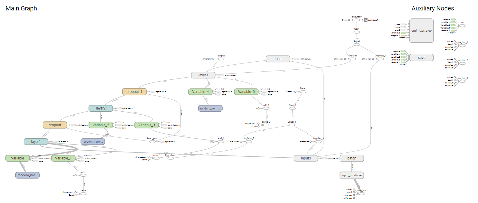
Figure 6: The Construction of Feedforward Neural Network

In this paper, we use these indices in section 2.2 to evaluate the unsupervised and supervised models, such as control chart theory, isolation forest, polynomial regression, XGBoost and deep feedforward neural networks. The parameters of these models are in table 5 and table 6 is the experiment results. In DNN model, the graphs between loss, accuracy and iterations are in figure 7.

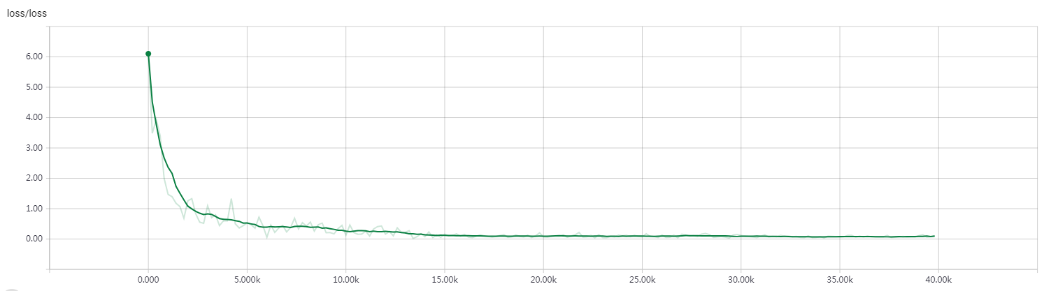
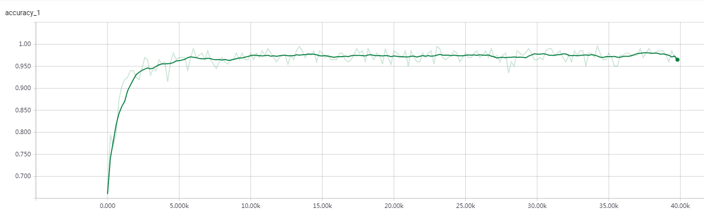
Figure 7: The Loss and Accuracy of DNN

Algorithms	Parameters
3-Sigma	None
EWMA Control Chart	coefficient = 3, alpha = 0.3
Polynomial Regression	degree = 4, threshold = 0.3
Isolation Forest	nestimator = 3, maxsample = ’auto’, contamination = 0.15
XGBoost	243 features, maxdepth = 10, eta = 0.05, gamma = 0.1, booster = ’gbtree’, objective = ’binary:logistic’, evalmetric = ’auc’
DNN-1	number of hidden layers = 2, number of elements in hidden layer = 50, activation function = Leaky ReLU, no dropout
DNN-2	number of hidden layers = 2, number of elements in hidden layer = 50, activation function = Leaky ReLU, dropout = 0.95

Table 5: Parameters of Models

Algorithms	TP	FN	FP	TN	Recall	Precision	F1-Score
3-Sigma	10524	702	1331	3178	70.5%	81.9%	75.8%
EWMA Control Chart	8981	2245	294	4215	93.5%	65.2%	76.8%
Polynomial Regression	9193	2033	579	3930	87.2%	65.9%	75.7%
Isolation Forest	9071	2155	364	4145	91.2%	65.8%	76.4%
XGBoost	11082	144	1039	3470	77.0%	96.0%	85.5%
DNN-1	11091	135	891	3618	80.2%	96.4%	87.6%
DNN-2	11100	126	852	3657	81.1%	96.7%	88.2%

Table 6: Experiments of Algorithms

iii.   Output of Hidden Layers as Features of Time Series

iii.1 Clustering of a Set of Time Series

In statistics, there are several clustering algorithms of clustering of time series, such as KMeans and hierarchical clustering. For example, pearson coefficient and dynamic time warping can be used to calculated the similarity between two time series, then we can get clusters of several time series based on similarity measures and feature engineerings of time series. In the paper, we use a trained neural network to calculate features of time series. More precisely, in our deep feedforward neural network, there are two hidden layers, the output of these two layers can be seen as the hidden features of time series, which is called "Time Series To Vector". For a trained neural network, we can get two hidden features from one time series, then we use clustering algorithms such as KMeans to get several clusterings. The figure 8 is the clustering result of time series with these two hidden features.

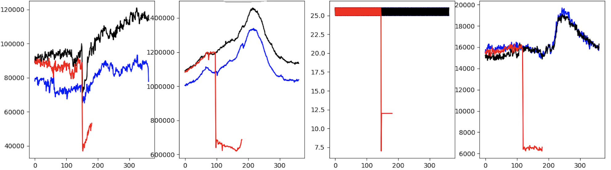
Figure 8: Clusters of Time Series

iii.2 Cosine Similarity between Two Time Series

In mathematics, there are many formulas to calculate similarity between two different time series, such as pearson coefficient, SAX, piecewise average aggregation. In this paper, we can also use the output of two hidden layers as the features of time series, then the cosine similarity between the output of hidden layers of two time series is a similarity measure between them. The performance of this similarity method can be seen in figure 9.

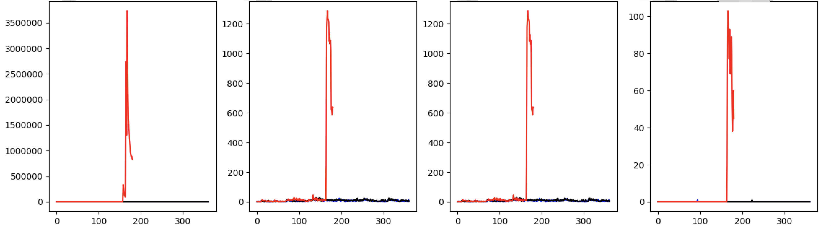
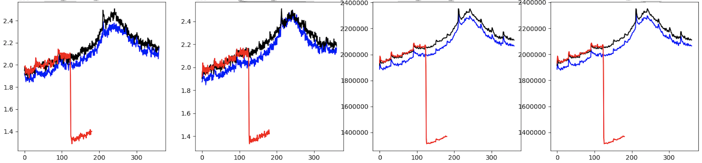
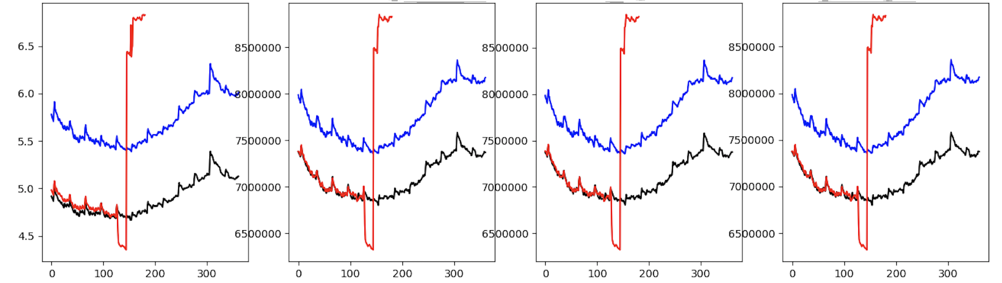
Figure 9: Three Similar Time Series of the First Time Series Every Line

V.   Conclusion

In conclusion, from the main theorem and experiments, deep feedforward neural network is a useful supervised model in time series anomaly detection, and it can get hidden features of time series from a trained neural network. Training a deep neural network is an end-to-end method which need only raw datasets and their corresponding labels. The performance metrics, such as precision, recall and F1-score, of deep feedforward neural network is better than XGBoost with feature engineering. The most important thing of the paper is that we do not need feature engineering in the process of training a feedforward neural network. After we get a trained neural network, the output of hidden layers of some time series can be seen as the hidden features of them, which can be called as "TimeSeries2Vec". Then we can use cosine similarity to calculate the similarity between two different time series or do clustering analysis from these hidden features. To the best of our knowledge, our system is the first anomaly detection framework based on deep neural network, and it do not need any feature engineering of time series, which is the biggest difference between ours and other supervised models.

Appendix A Appendix

In the section, we pay attention to prove the main theorem of the paper. The main theorem is as follows:

Theorem.

Suppose $n\geq 1$ is a positive integer, there exists a deep feedforward neural network $D$ such that for any real time series $\mathbf{X}_{n}=[X_{1},\cdots,X_{n}]$, the input and output of $D$ are $\mathbf{X}_{n}$ and the features of $\mathbf{X}_{n}$ in Table 2, respectively.

Proof.

At the beginning, we will show that some basic calculations, such as addition, subtraction, absolute value, maximum, minimum and average, can be construct from feedforward neural networks. More precisely,

$$\text{add}(x,y) = x+y,$$

$$\text{sub}(x,y) = x-y,$$

$$\text{abs}(x) = ReLU(x)+ReLU(-x),$$

$$\max(x,y) = (x+y+|x-y|)/2,$$

$$\min(x,y) = (x+y-|x-y|)/2,$$

$$\text{average}(x_{1},\cdots,x_{n}) = (x_{1}+\cdots+x_{n})/n,$$

where $\text{ReLU}(x)=\max(x,0)$. Since neural network contains matrix summation and multiplication, we easily see the above functions can be written as the form of feedforward neural networks in figure 10.

Figure 10: Basic Calculation of Real Numbers

From above, we have already known that some basic calculation between two real numbers can be constructed by feedforward neural network. Next we will prove that these features in Table 2 can also be constructed by feedforward neural networks. Suppose there is a time series $X_{n}=[x_{1},\cdots,x_{n}]$ with length $n$, some features are defined as followings:

$$\max:$$

$$\max_{1\leq i\leq n}\{x_{1},\cdots,x_{n}\}$$

$$=\max\{x_{1},\max\{x_{2},\cdots,\max\{x_{n-1},x_{n}\}\}\},$$

$$\min:$$

$$\min_{1\leq i\leq n}\{x_{1},\cdots,x_{n}\}$$

$$=\min\{x_{1},\min\{x_{2},\cdots,\min\{x_{n-1},x_{n}\}\}\},$$

$$\mbox{average}:\sum_{i=1}^{n}x_{i}/n,$$

$$\mbox{difference}:x_{2}-x_{1},\cdots,x_{n}-x_{n-1},$$

$$\mbox{integration}:\sum_{i=1}^{n}x_{i},$$

$$\mbox{absolute sum of changes}:\sum_{i=1}^{n-1}|x_{i+1}-x_{i}|,$$

$$\mbox{mean change}:\sum_{i=1}^{n-1}(x_{i+1}-x_{i})/n=(x_{n}-x_{1})/n,$$

$$\mbox{mean second derivative central}:$$

$$\sum_{i=1}^{n-2}(x_{i+2}-2x_{i+1}+x_{i})/(2n).$$

From basic calculation between real numbers, the above features can be also constructed by feedforward neural networks. Recall that Simple Moving Average, Weighted Moving Average, Exponentially Weighted Moving Average algorithms are defined as

$$SMA_{n}(w) = \frac{\sum_{k=1}^{w}x_{n-w+1}}{w}$$

$$= \frac{x_{n-w+1}+\cdots+x_{n}}{w},$$

$$WMA_{n}(w) = \frac{\sum_{k=1}^{w}k\cdot x_{n-w+k}}{\sum_{k=1}^{w}k}$$

$$= \frac{2\cdot\sum_{k=1}^{w}k\cdot x_{n-w+k}}{w(w+1)},$$

$$EWMA_{j}(\alpha) = x_{1},\mbox{ if }j=1,$$

$$EWMA_{j}(\alpha) = \alpha\cdot x_{j-1}+(1-\alpha)\cdot EWMA_{j-1},\mbox{ if }j\geq 2.$$

where $w\geq 1$ is the window size and $\alpha\in[0,1]$ is a factor. The fitting features from these statistical models are constructed by the subtraction between fitting values from these models and real values. More precisely, the formulas of fitting features are

$$SMA_{n}(w)-x_{n},\mbox{ where }w=10,20,30,40,50,$$

$$WMA_{n}(w)-x_{n},\mbox{ where }w=10,20,30,40,50,$$

$$EWMA_{n}(\alpha)-x_{n},\mbox{ where }\alpha=0.2,0.4,0.6,0.8.$$

From its definition, EWMA can be written as

$$EWMA_{n}(\alpha)$$

$$= \alpha\cdot x_{n-1}+(1-\alpha)\cdot EWMA_{n-1}$$

$$= \alpha\cdot x_{n-1}+\alpha(1-\alpha)x_{n-2}+\alpha(1-\alpha)EWMA_{n-2}$$

$$= \alpha\cdot x_{n-1}+\alpha(1-\alpha)x_{n-2}+\cdots+\alpha^{n-2}(1-\alpha)x_{1}.$$

In figure 11, we have already shown that how to construct fitting features of time series from simple moving average, weighted moving average, exponentially moving average algorithms.

Figure 11: Fitting Features of Time Series

Next, we will prove that simple threshold, count above mean and count below mean can be written as the form of feedforward neural network. First, the features of simple threshold for a fixed real number $a$ are defined as, i.e.

$$\mathcal{I}_{\{x\geq a\}}=\begin{cases}&1,\mbox{ if }x\geq a,\\ &0,\mbox{ else }x<a.\end{cases}$$

and

$$\mathcal{I}_{\{x<a\}}=\begin{cases}&0,\mbox{ if }x\geq a,\\ &1,\mbox{ else }x<a.\end{cases}$$

Let

$$f_{a}(x) = \sigma(-2\cdot 10^{4}\cdot ReLU(-x+a)+10),$$

$$g_{a}(x) = \sigma(-2\cdot 10^{4}\cdot ReLU(x-a)+10),$$

where $\sigma$ denotes the sigmoid function, i.e. $\sigma(x)=1/(1+\exp(-x))$. Then if $x>a$, then $f_{a}(x)=\sigma(10)\approx 1;$ if $x<a-10^{3}$, then $f_{a}(x)=\sigma(-2\cdot 10^{4}\cdot(a-x)+10)<\sigma(-10)\approx 0$. Therefore, $f_{a}(x)\approx\mathcal{I}_{\{x\geq a\}}$. Similarly, the proof of $g_{a}(x)\approx\mathcal{I}_{\{x<a\}}$ is the same as before.

Second, the construction of count above mean and count below mean are based on $f_{a}(x)$ and $g_{a}(x)$. More precisely, count above mean denotes the number of the time series $[x_{1},\cdots,x_{n}]$ which are larger than the average value of time series. Similarly, count below mean denotes the number of the time series $[x_{1},\cdots,x_{n}]$ which are less than the average value of time series. In figure 12, we have already shown that how to construct these two features from $f_{a}(x)$ and $g_{a}(x)$. Hence, we have already proven the main theorem of the paper.

Figure 12: Count Features of Time Series

∎

- [1] D. C. Montgomery, Introduction to statistical quality control. John Wiley & Sons, 2007.
- [2] J. Contreras, R. Espinola, F. J. Nogales, and A. J. Conejo, “Arima models to predict next-day electricity prices,” IEEE transactions on power systems, vol. 18, no. 3, pp. 1014–1020, 2003.
- [3] H. Z. Moayedi and M. Masnadi-Shirazi, “Arima model for network traffic prediction and anomaly detection,” in Information Technology, 2008. ITSim 2008. International Symposium on, vol. 4, pp. 1–6, IEEE, 2008.
- [4] B. Pincombe, “Anomaly detection in time series of graphs using arma processes,” Asor Bulletin, vol. 24, no. 4, p. 2, 2005.
- [5] C. Chatfield and M. Yar, “Holt-winters forecasting: some practical issues,” The Statistician, pp. 129–140, 1988.
- [6] C. C. Aggarwal, “Outlier analysis,” in Data mining, pp. 237–263, Springer, 2015.
- [7] F. T. Liu, K. M. Ting, and Z.-H. Zhou, “Isolation forest,” in 2008 Eighth IEEE International Conference on Data Mining, pp. 413–422, IEEE, 2008.
- [8] Y. Chen, X. S. Zhou, and T. S. Huang, “One-class svm for learning in image retrieval,” in Image Processing, 2001. Proceedings. 2001 International Conference on, vol. 1, pp. 34–37, IEEE, 2001.
- [9] D. Liu, Y. Zhao, H. Xu, Y. Sun, D. Pei, J. Luo, X. Jing, and M. Feng, “Opprentice: Towards practical and automatic anomaly detection through machine learning,” in Proceedings of the 2015 Internet Measurement Conference, pp. 211–224, ACM, 2015.
- [10] H. Xu, W. Chen, N. Zhao, Z. Li, J. Bu, Z. Li, Y. Liu, Y. Zhao, D. Pei, Y. Feng, et al., “Unsupervised anomaly detection via variational auto-encoder for seasonal kpis in web applications,” in Proceedings of the 2018 World Wide Web Conference on World Wide Web, pp. 187–196, International World Wide Web Conferences Steering Committee, 2018.
- [11] J. D. Hamilton, Time series analysis, vol. 2. Princeton university press Princeton, NJ, 1994.
- [12] W. Rudin et al., Principles of mathematical analysis, vol. 3. McGraw-hill New York, 1976.
- [13] W. Rudin, Real and complex analysis. Tata McGraw-Hill Education, 2006.
- [14] Baidu, An Integrated Experimental Platform for time series data anomaly detection., 2017. https://github.com/baidu/Curve.
- [15] Microsoft, Anomaly detection analysis and labeling tool, specifically for multiple time series (one time series per category)., 2018. https://github.com/Microsoft/TagAnomaly.
- [16] P. Malhotra, L. Vig, G. Shroff, and P. Agarwal, “Long short term memory networks for anomaly detection in time series,” in Proceedings, p. 89, Presses universitaires de Louvain, 2015.