Statistical learning of geometric characteristics of wireless networks ††thanks: A. Brochard is with the Huawei R&D France and Inria/ENS, Paris, France; B. Błaszczyszyn is with Inria/ENS, Paris, France; S. Mallat is with College de France and ENS Paris, France; S. Zhang is with Peking University, Beijing.
Abstract
Motivated by the prediction of cell loads in cellular networks, we formulate the following new, fundamental problem of statistical learning of geometric marks of point processes: An unknown marking function, depending on the geometry of point patterns, produces characteristics (marks) of the points. One aims at learning this function from the examples of marked point patterns in order to predict the marks of new point patterns. To approximate (interpolate) the marking function, in our baseline approach, we build a statistical regression model of the marks with respect some local point distance representation. In a more advanced approach, we use a global data representation via the scattering moments of random measures, which build informative and stable to deformations data representation, already proven useful in image analysis and related application domains. In this case, the regression of the scattering moments of the marked point patterns with respect to the non-marked ones is combined with the numerical solution of the inverse problem, where the marks are recovered from the estimated scattering moments. Considering some simple, generic marks, often appearing in the modeling of wireless networks, such as the shot-noise values, nearest neighbour distance, and some characteristics of the Voronoi cells, we show that the scattering moments can capture similar geometry information as the baseline approach, and can reach even better performance, especially for non-local marking functions. Our results motivate further development of statistical learning tools for stochastic geometry and analysis of wireless networks, in particular to predict cell loads in cellular networks from the locations of base stations and traffic demand.
I Introduction
Design, performance evaluation and control of wireless networks are facing rapid increase in complexity, due to more and more dense deployment of the classical cellular networks and the advent of the Internet of things. It is clear that engineering of these networks needs to make more systematic use of the data massively collected in operational conditions, thus opening this domain to possible applications of machine learning methods.
While advanced signal processing techniques at the link layer already integrate elements of artificial intelligence (like belief propagation in Bayesian networks for low-density parity-check and turbo codes) it is more seldom to see them used at higher levels, in particular at the network layer. The data corresponding to this layer (e.g. base station locations, their characteristics and performance metrics, user distribution and QoS metrics) have geometric structure, reflecting (usually two-dimensional) geographic network deployment. It is thus natural to ask questions regarding pertinence of the rapidly developing machine learning tools for image analysis and related fields to this new domain of applications.
I-A Statistical learning of marks of point processes
In this paper we pose and address to the following fundamental problem of statistical learning of marks of point processes: An unknown marking function depending on the relative locations of points produces characteristics of these points, called marks. One aims at learning this function from the examples of point patterns with observed marks in order to predict unknown marks for new point patterns.
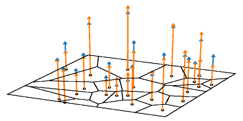
Our particular motivation comes from the problem of learning of the dependence of the cell loads in wireless networks on the geometry of base stations (and possibly of the traffic demand) directly from real data collected in the existing, operational networks, to predict loads of base stations for different base station positioning and/or different traffic demand; see more details in Section I-C. In this founding work, we consider some simple, generic marks, often appearing in this context. They are produced by the standard shot-noise interference model, the nearest neighbour distance, and some characteristics of the Voronoi cells (cf Figure 1). Our goal is to understand the amenability of marks representing different types of dependence on point patterns to the proposed statistical learning approach.
I-B Learning via local or global geometry representation
The learning (interpolation) of the marking function in the original problem does not seem amenable to any direct statistical approach, due to the structure of the space of marked point measures. To overcome this difficulty, we need some suitable representation of the geometry of point patterns, and we propose two approaches in this regard.
As a baseline, we propse to estimate the mark of each point using the statistical regression model based on the local distance matrix of a suitable chosen vicinity of this point. In this relatively simple approach, the training data set consists of an ensemble of central, marked points surrounded by some number, say , of their (non-marked) neighbours. If no a’priori information regarding the dependence region of the marking function is available, one needs to choose using cross validation. Observe that the dimension of the domain of the interpolated marking function (local distance matrix) increases as . For highly non-local marking functions (e.g. related to power-law shot-noise function), one might need to take large, proportional to the total number of points, making this baseline approach not efficient.
When the marks have non-local dependence, or when we have no prior knowledge of the dependency range, we further propose to use the scattering moment representation [1] to capture the geometry of marked point patterns. It is a discrete family of nonlinear and noncommuting operators, computing at different scales the modulus of a wavelet transform of the one- or higher-dimensional signal (e.g. image). Applied to the signal observed in a finite window, they are proven to be Lipschitz-continuous with respect smooth (class ) signal diffeomorphisms. As the window size increases, they become invariant with respect to the translation of the signal. They can be also made rotation invariant. These invariance and stability properties make them useful in signal processing, in particular in relation to statistical learning. Indeed, if the information content of an image typically is not (strongly) affected by translations, rotations, and small deformations, similar properties of the signal representation allows one to capture this content in a more concise way, and hopefully learn its intrinsic structure from a smaller number of signal samples. The pertinence of this approach has already been demonstrated in various contexts.
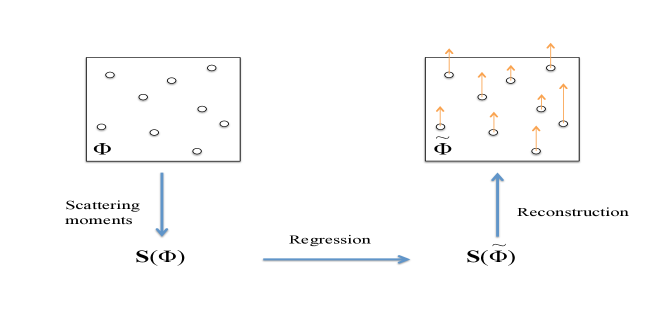
Using the scattering moments to represent marked point processes, our learning problem can be addressed in the following two steps (also depicted on Figure 2):
-
•
We build a statistical regression model on scattering moments of the marked point patterns with the explanatory variables being the scattering moments of the non-marked point patterns. This model is computed on the training data consisting of point patterns with observable marks and is meant to be used to estimate the (marked) scattering moments of new point patterns, for which marks are not observed.
- •
This approach scales much better with the total number of points. Indeed, the number of scattering moments capturing the global geometry grows logarithmically with this number. However, it may suffer from possible errors introduced in the reconstruction phase (absent in the benchmark approach). The overall benefits of the scattering approach become significant for highly non-local marking functions.
In general, the quality of the regression of the scattering moments depends on the sensitivity of the marking function to small point pattern deformations — a concept not yet well understood in point process literature (e.g. the nearest neighbour distance seems to be more sensitive than shot-noise). On the other side, in the reconstruction phase (recovering of marks from the true or estimated scattering moments) significant errors consist in swaping a large and a small mark of two neighbouring points (not leading to a significant modification of the considered first scattering moments). The quality of this phase of the approach depends thus on the existence of clusters of points in point patterns — a problem already studied in the literature; cf Section I-C. The Poisson point process, considered in this paper, exhibits a baseline type of clustering.
I-C Related works
Stochastic-geometric study of cellular networks expands rapidly in recent years primarily through analytic results regarding Poisson network models [4]. Performance evaluation of operational wireless cellular networks, in particular the quality of service perceived by users in function of the traffic demand, is a complex problem involving stochastic and geometric modelling of several network layers. A key element of this problem is the analysis of the cell loads, which non trivially depend on the geometric configuration of serving base stations and their traffic demands, and capture in concise way the quality of service offered by the individual cells. A detailed physical model of cell loads was proposed [5] and revisited in [6, 7, 8] including the validation with respect to some data collected in operational networks.
Recently, the prediction of the cell loads has been the subject of a machine learning study published in [9], though not as the geometric problem posed in our paper. Indeed, in this earlier paper the number and the locations of base stations are fixed, and the problem consist in learning the loads of this given configuration of stations in function of their traffic demands. This (non-geometric) problem is cast and solved in the framework of monotone interpolation of Lipschitz functions.
The problem formulated and studied in our paper allows one to address the completely orthogonal question of learning of the cell loads, given constant traffic demand, in function of the geometry of the network. Combining the two approaches, left for the future work, will allow one to predict the performance of new geometric configurations on base stations and traffic demand by collecting the cell load data in existing, operational networks, thus offering an alternative to building and solving complex physical models.
Observe that, even for a fixed number of base stations, the two dimensional location of each base station on the plane makes our geometric argument of the marking function have two times higher dimension than the one considered in [9]. Using wavelet scattering transforms allows one to leverage geometric invariants, such as translation and rotation invariance with respect to the locations of stations, and thus significantly reduce the representation dimension. Scattering moments have been proven useful in this context in a number of tasks such as quantum molecular energy prediction [10] or texture classification [11, 12].
Geometric marks (called also score functions) have received a lot of attention in stochastic geometry and spatial statistics, where they represent some interaction of a given point with the whole point pattern. If this interaction is local in some sense, and the underlying point process exhibits some decay of correlations, then it is possible to establish asymptotic results (including central limit theorems) regarding the sums of the geometric marks observed in increasing window; cf e.g. [13, 14, 15]. These results can be used to study large-scale asymptotic of the scattering moments as in [16].
It was mentioned in the introduction that the quality of reconstruction of the marks depends on whether point process is regular or clusters its points. These notions are formalised in [17, 18], and it is argued that Poisson point process exhibits some reference type of point clustering, to which more regular point processes (e.g. determinantal ones) and more clustering ones (e.g. permanental and Cox processes) can be compared in terms of the performance of different geometric characteristics.
The remaining part of this paper is organized as follows
In Section II we describe several models of geometric marks and formulate the problem of their statistical learning. In Section III we present our main approach proposed to solve this problem, based on scattering transforms of marked point processes. We also describe the benchmark approach. The numerical results of both approaches applied to the considered mark models are presented in Section IV.
II Geometric characteristic of wireless networks
In stochastic-geometric modeling of wireless networks, one usually represent locations of transmitters/receivers as points of a point process, and their characteristics as marks. These characteristics can depend not only on the given transmitter/receiver (as e.g. the type of the base station in heterogeneous cellular networks or the local density of users in the vicinity of this station) but also on (at least) local geometry of the network (as e.g. the surface of the cell served by the base station, the extra-cell interference). These marks, called in what follows geometric marks, are in the center of our interest in this paper.
II-A Geometric marks
More formally, let be a simple ( for ) , stationary (having distribution invariant by any translation) point process on the Euclidean plane . Recall, is a random object on the space of locally finite counting measures on with a suitable -field; cf [19]. Consider a (measurable) marking function defined on . Assume is invariant with respect to translations on the plane, i.e., for any , where is the translation of the counting measure (of its atoms) by the vector . We will call geometric mark of the point of . Note that is a stationary marked point process.
In what follows we briefly remind a few basic examples of geometric marks that will be considered in the remaining part of this paper. For better understanding of the context we interpret points as locations of base stations of some cellular network.
II-A1 Shot-noise
For and , let be a shot-noise functional with some non-negative response function of the distance between and . Taking to be the standard power-law path-loss model with the path-loss exponent , we recognize in the total power (usually interpreted as interference) received at the station from other stations of the network, all transmitting with a unit power.
II-A2 Nearest neighbour distance
Let be the the distance from to its nearest point in . Similarly one can define distances to successive neighbours of in .
II-A3 Voronoi cell surface area and moment of inertia
Denote by the Voronoi cell of the point in . It is the polygon representing all locations on the plane closer to than to any other point in . This is a fundamental cell model for cellular networks. We will consider two basic numerical characteristics of the Voronoi cells: the surface area and the moment of inertia . The marks and can be interpreted as very simple proxies to the traffic demand and the cell load of the station (the latter assuming user peak-bit rate satisfies the inverse square law with respect to its serving station; cf [4, Section 4.1.8]).
II-A4 Voronoi shot-noise
By this we call the marks defined as follows: . Having interpreted shot-noise of Section II-A1 as the interference received at the station from all other stations transmitting a unit power, can be also interpreted as the interference, however with the stations transmitting the signals with the power proportional to their Voronoi cells. (Similar kind of dependence, with more complicated expressions, can be recognized the cell load model of [5].)
II-B Problem formulation
Let us now formulate the main problem studied in this paper, that is the problem of learning of geometric marks. Suppose the marking function is not known explicitly. One observes only some realizations of the marked point process with points restricted to some finite observation window . Denote these realizations by , with , . They form a training set of data. The problem consists in learning the function from the training set so as to be able to calculate approximations of the unobserved marks for a new realization of (only points) of the point process .
III Statistical learning of geometric marks
In this section we propose a solution to the learning problem formulated in Section II-B. Our main approach, described in Section III-B, uses a wavelet based representation of marked point patterns. It is presented in Section III-A. Finally, in Section III-C we describe an alternative method, based on a distance matrix representation of point neighbourhoods, used as a benchmark approach for our numerical study in Section IV.
III-A Scattering moments of marked point processes
Following [16], now we shall briefly present the wavelet scattering transform of marked point processes on the plane .
Let be a continuous, bounded, complex function on of zero average and such that for . It is customary to normalize it so that . We call (two-dimensional) mother wavelet.
Example III.1
Two dimensional Morlet wavelet has the following form , where is the imaginary unit and is the scalar product of some nonzero vector parameter , called spatial frequency, with . Note that it is not normalized and, moreover, it is only approximately zero average when is large enough; typically ; cf [20].
Consider a family of dilated, and rotated wavelets : for and let , where deontes the rotation of by the angle with respect to the origin on the plane (and the factor in the first exponent corresponds to the dimension ).
Let be a simple stationary marked point process with points and some real marks . The wavelet transform of at scale and angle , , , is defined as the following (stationary, complex) random filed on :
| (1) | ||||
| (2) |
The wavelet transform of a (non-marked) point process is defined by (2) with unit marks .
The first order scattering moments of , at scale , and angle , are defined as the expectation of the modulus of the corresponding wavelet transform (without loss of generality evaluated at the origin)
| (3) |
and similarly for the non-marked point process .
The second order scattering moments , , , are defined by induction as the first order scattering moments at scale and angle of the random measure on admitting the modulus of the wavelet transform at scale and angle for density (this measure replaces the projecton of the point measure on in (1))
| (4) |
Higher order scattering moments are defined by induction (but they are not used in this paper). Scattering moments have not yet been fully theoretically studied on the ground of the theory of point processes. Some asymptotic properties at small and large scale ( and respectively) can be established, extending results presented in [16]. 111In particular, it is not known to what extend the scattering moments characterize the distribution of the point process. Note that higher order factorial moment measures (their densities, if exist, are called the correlation functions) are known to characterize the distribution of the simple point process having finite exponential moments. The following two observations can be made regarding the relation between the correlation functions and the scattering moments. Note that the wavelet transforms (2) are linear functions (shot-noise functionals) of the (marked) point process; in other words they are first-order -statistics of ; cf [21, Section 12.3]. The fact that scattering moments are defined via the moduli of the wavelet transforms makes them dependent on all higher-order correlation functions of : the factorial moment expansions [22, 23] of involve all moment measures (in contrast to the square norm of the wavelet transforms, which can be represented using the first and second-order -statistics and thus their expansion involves only the first two correlation functions). Consequently, already the first scattering moments are supposed to capture more information regarding the intrinsic dependence of the points than just the pairwise correlations. We shall see in our numerical study that this information allows one for an efficient recovery of some geometric marks which do depend on higher order correlations, e.g, the Voronoi cell characteristics. Even if we do not know whether the (higher-order) scattering moments characterize the distribution of the point processes, being a discrete family of numbers (provided a suitable discretization of ) they are supposed to capture the point correlations in a more concise way than the higher-order correlation functions. In practice, a reasonable estimation of the scattering moments requires much less examples of point patterns than the estimation of the moment mesures.
III-A1 Empirical scattering moments
For a given realization of observed in a finite window , empirical scattering moments and are obtained replacing the expectation in (3) and (4) by the empirical averaging of the fileds and , resepectively, over . When increses suitable to the whole plane, these (empirical) moments become asymptotically non-biased estimators of and , respectively, provided is ergodic, at least when the mother wavelet has finite support; cf ergodic theorem for point processes [19, Theorem 13.4.III]. For some other properties of the scattering moment estimators see [16, Section 5.1].
To avoid boundary effects and enforce the translation invariance of the empirical scattering moments calculated over finite rectangular window it is customary to map with the observerd points on the torus.
It is natural to restrict the scale parameter to a finite window . The minimal scale is chosen such that the support of separates points (making close to the empirical mean times the first norm of the mother wavelet). It does not depend on the angle . The maximal scale is chosen such that covers the whole window. For the second order scattering moments, it is natural to consider . Regarding the choice of the angles in both families of scattering moments, it is natural to consider some common symmetric constellation of angles .
Thus, the first and second empirical scattering moments calculated on form finite-dimensional (column) vectors. We denote by , and , respectively, the vector of the first moments and the joint vector of the first and second moments. If no ambiguity, for simplicity, in what follows we shall call them just scattering moments of .
III-B Learning of marks via scattering moments
Recall from Section II-B that our goal is to learn the marking function (or depending on the auxiliary marks) from the training set of data, which consists of examples of realizations of a marked point process in a finite window, in order to calculate approximations of the unobserved marks for a new realization of the (non-marked) point process . Note that this problem consists in the interpolation of the function on the space and due to the complexity of this space is not amenable to any direct statistical approach. To overcome this difficulty, we map this original problem to some finite dimensional regression problem and solve it using classical tools.
More specifically, in our main approach, we shall capture the function through relation between the vector of the first order scattering moments of the marked point pattern and the two moments of the non-marked one. This relation is established using some known regression models described in Section III-B1. In order to be able to use it to estimate marks , we need next to solve an inverse problem described in Section III-B2. It consists in reconstructing marks from the regressed scattering moments (approximating unknown ) knowing also locations of points .
III-B1 Regression
Let and , , be the vectors of the (empirical) scattering moments calculated for the training data set consisting of realizations of the point process , where points and points with their marks are considered, respectively; cf Sections II-B and III-A1. Our goal is to find a common relation between and for all sample , and the simplest possible one is a linear relation represented by some matrix and vector such that
| (5) |
This is a linear regression problem briefly presented in Section III-B1. If the linear function does not allow one to capture the dependence, we can use the kernel regression or more advanced machine learning tools. In this paper, we focus on the linear ridge regression.
Linear ridge regression
To find the linear relation (5) we will use (linear) ridge model; cf [24, Section 7.5]. For , denote by the line of the matrix (5); it corresponds to the scattering moment in at scale and angle , and similarly the component for the vector . Let be the -component of . The ridge model consists in minimizing the regularized sum of the squared residuals
for some (Tikhonov) regularization parameter , chosen by the cross-validation (to minimize this squared residuals on the validation set: a subset of the training set), where is the Euclidean norm. This model, admits a well known explicit solution in the form
| (6) |
where is the matrix with lines appended with the first column of 1’s, is the column vector with elements , , is the appropriate identity matrix and stands for the matrix transpose.
Using (6) one can calculate approximations of the scattering moments of a new marked configuration observing only its points
where is the vector of the 2nd order scattering moments calculated on (points-only). Remember, expression (6) requires tuning of the regularization parameters usually needed in high dimensional regression problems when the matrix is not invertible. The ordinary least square (OLS) estimator corresponding to is not performing well in this case.
III-B2 Reconstruction
Using linear ridge we calculate approximations of the scattering moments of a new marked configuration observing only its points . Denote the whole vector of by . From we estimate (reconstruct) unknown marks of looking for a solution to the following minimization problem
| (7) |
where we minimize over all arbitrarily marked configurations sharing the points with given (hence over unknown marks) and denotes the scattering moment calculated for . It should be noted that (7) is a non convex optimization problem. To solve it we use L-BFGS-B algorithm, which is a limited-memory algorithm for solving large nonlinear optimization problems subject to simple bounds on the variables. It is intended for problems in which information on the Hessian matrix is difficult to obtain, or for large dense problems; cf [2, 3].
III-C Learning via local distance representation
In this approach, considered as a benchmark, we consider each marked point of each realization , , of the training set; cf Section III-B1, along with some neighborhood, as one element of the new training data set. In this case the training set consists of point patterns having a marked point the center, surrounded by some neighboring points. Using the the linear ridge regression described in Section III-B1, mutatis mutandis, we regress the marks of those central points with respect to the vectors containing all inter-point distances in the considered point neighborhood, ordering the points according to the distance to the central point and flattening the distance matrix in (say) raw major order. Note that, in this approach, there is no reconstruction phase, as the marks are directly approximated. The main parameter of this approach is the number of points taken into account in the neighborhood.
IV Numerical results
In this section we provide the details of our numerical study of the main problem of this paper, namely statistical learning of geometric marks of point processes. We begin by describing some general assumptions and procedures.
IV-A General numerical framework
IV-A1 Scattering moment approach
For our numerical experiments, for each specific geometric model, we create a data set (denote it by ) of Poisson point patterns (with constant intensity to be specified) using the R software and its package Spatstat for point process analysis [25]. The points are considered in the unit square window and their marks are analytically computed (according to the given model) using Spatstat with the window mapped to the torus, thus leading to the marked point patterns , . The size of the data set is marked point patterns.
The (empirical) scattering moments are computed on these point patterns (with and without marks) using ScatNet software [26] developed in Matlab (no Spatstat implementation is available yet). It uses a zero-mean variant of the Morlet wavelet; cf Example III.1. This latter software working on raster images, we convert each marked point pattern of into images of size pixels (removing images with points corresponding to the same pixel).
The following family of scattering moments are computed. We assume the smallest scale . At this scale the first scattering moments correspond to the empirical mean measure and do not depend on the angle ; cf Section III-A1. We take and following constellation of 8 angles for all scales . Thus, there are first order scattering moments (dimension of the regressed vectors equals to 57) and of the moments of the second order (thus making the dimension of the explanatory vectors equal to ).
We use the linear ridge regression described in Section III-B1 on the data set . To optimize the regression parameters we make 5-fold cross-validation [24, Section 1.4.8] on .
Having calculated the estimators of the first marked scattering moments for the point patterns in the test set we use L-BFGS-B algorithm [2, 3] to solve the inverse problem (7), that is to reconstruct the marks. This is a steepest descent algorithm for which it is important to optimize (via cross-validation) the number of iterations; to be explained in Section IV-C1. Using a rule of thumb (no formal cross-validation) we fix the number of steps so as to minimize the mean square error (MSE) on the test data set.
IV-A2 Benchamrk
As explained in Section III-C, for every image in the data set , we consider each point of the image, along with its neighbours as an element of a new data set . More precisely, we take the first of points of the images of and create with neighbours of the chosen point. The value of depends on range of dependence of a given mark model; it is experimentally discovered for each mark, as will be explained in Section IV-C2. We use to regress directly, using the linear ridge regression method, the (one dimensional) central point marks with respect to the vector of dimension of the local distance matrix. There is no reconstruction phase in the benchmark.

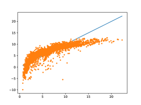
(a) (b) (c)
| method | scattering | scattering | exact | bench- |
|---|---|---|---|---|
| scatt. | mark | |||
| RMSE | 1.99 | 1.98 | 1.64 | 1.98 |
| NRMSE1 | 9.21e-2 | 9.15e-2 | 7.56e-2 | 9.15e-2 |
| NRMSE2 | 3.32e-1 | 3.29e-1 | 2.75e-1 | 3.29e-1 |

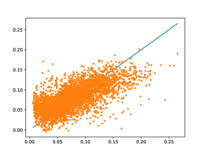
(a) (b)
| method | estimated scatt. | exact scatt. | benchmark |
|---|---|---|---|
| RMSE | 3.14e-2 | 2.06e-2 | – |
| NRMSE1 | 1.21e-1 | 7.94e-2 | – |
| NRMSE2 | 3.94e-1 | 2.58e-1 | – |
IV-A3 Validation methodology
For testing of the main (scattering moment) approach, we produce an independent data set of 100 marked point pattern realizations and we use the first 100 points of this set for the benchmark approach.
For all points in the respective test sets, we compute Q-Q plots and the root mean square error (RMSE), the normalized RMSE with normalization by the range () of the marks (NRMSE1), and the normalized RMSE with normalization by the mean of the marks (NRMSE2).
In order to study the quality of the representation of the mark point patterns by their first order scattering moments (independently of the regression), we also perform the reconstruction of marks III-B2 directly from the exact (and not regressed) scattering moments . Note, these latter are not “exact” marks but marks reconstructed from exact empirical scattering moments of the given point pattern. The gap between them and the marks reconstructed from the regressed moments allows one to apprehend the error introduced by the regression.
IV-B Results
We now present our numerical study of different mark models presented in Section II. The observed results are discussed in Section IV-C.
IV-B1 Shot-noise
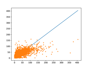
We consider shot-noise marks introduced in Section II-A1 with the response function . For this example the data set consists of realizations of Poisson point process of intensity 40 (recall, always considered the unit square window). In order to observe how the performance of our approach depends on the size of the data set and on two different regression methods, we first use only elements of as the training set for the linear ridge regression to estimate the scattering moments of the marked point patterns. Next, we use the whole training set, with linear ridge regression. The neighborhood for the benchmark is . The number of iterations for the reconstruction from the exact scattering moments and estimated ones is taken, respectively, 30 and 4; see Section IV-C1 for the explanation.
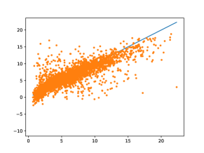
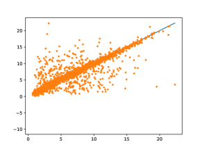
Figure 3 presents an example of the reconstruction of marks of one given image by the main method and Q-Q plots for various reconstruction variants. Table I presents reconstruction errors. Recall the Q-Q plot (c) and the last column of the table represents the error of the reconstruction of the marks from the exact (and not regressed) scattering moments.
IV-B2 Nearest neighbour distance
The data set for this example is also made of 10000 realizations of a Poisson point process with intensity 40. In this case, in On Figure 4 and in Table II we only show the results for the entire training set. For this mark model we do not consider the benchmark, because the nearest neighbour distance is equal to the first element of the distance matrix. Thus, the scattering moment approach cannot do better. The number of iterations for the reconstruction from the exact scattering moments and estimated ones is taken, respectively, 250 and 8.
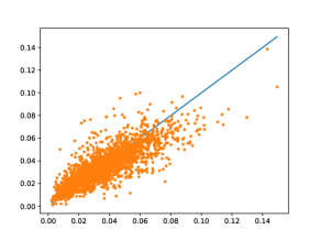
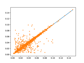
IV-B3 Voronoi cell surface area

(a) (b) (c)
| method | estimated scatt. | exact scatt. | benchmark |
|---|---|---|---|
| RMSE | 9.71e-3 | 7.33e-3 | 9.61e-2 |
| NRMSE1 | 6.60e-2 | 4.98e-2 | 6.53e-2 |
| NRMSE2 | 2.87e-1 | 2.16e-1 | 2.85e-1 |
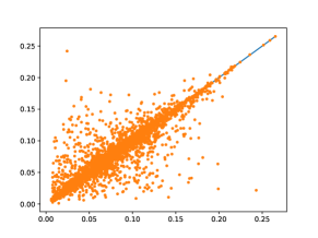
For this example, the training set consists of 10 000 realizations of Poisson point process with intensity 30. The reconstruction results are presented on Figure 5 and in Table III. The neighborhood for the benchmark is very large (more than the average number of points) because the sum of the areas of the Voronoi cells in the finite window is constant equal to the total window surface area, which introduces a strong global dependence for this mark. The number of iterations for the reconstruction from the exact scattering moments and estimated ones is taken, respectively, 30 and 6.
IV-B4 Voronoi cells moment of inertia
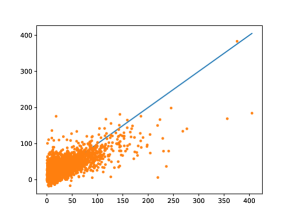
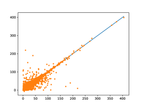
For this example, similarly to the previous example, the training set consists of 10 000 realizations of a Poisson point process with intensity 30. The results are presented on Figure 6 and in Table IV. The neighborhood for the benchmark is (note that the global dependence specific for the Voronoi surface area does exist here). The number of iterations for the reconstruction from the exact scattering moments and estimated ones is taken, respectively, 150 and 8.

(a) (b) (c)
| method | estimated scatt. | exact scatt. | benchmark |
|---|---|---|---|
| RMSE | 2.42e-4 | 1.37e-4 | 2.65e-4 |
| NRMSE1 | 5.98-2 | 3.39e-2 | 6.53e-2 |
| NRMSE2 | 7.12e-1 | 4.04e-1 | 7.74e-1 |
IV-B5 Voronoi shot-noise
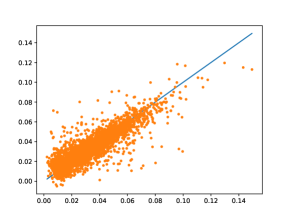
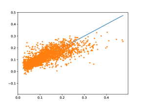
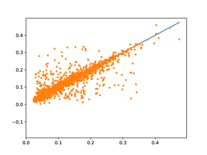
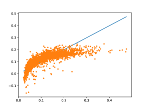
For this example, similarly to the previous example, the training set consists of 10 000 realizations of a Poisson point process with intensity 30. The results are presented on Figure 7 and in Table V. The neighborhood for the benchmark is . The number of iterations for the reconstruction from the exact scattering moments and estimated ones is taken, respectively, 50 and 5.

(a) (b) (c)
| method | estimated scatt. | exact scatt. | benchmark |
|---|---|---|---|
| RMSE | 4.17e-2 | 3.02e-2 | 4.29e-2 |
| NRMSE1 | 9.24-2 | 6.69e-2 | 9.50e-2 |
| NRMSE2 | 3.76e-1 | 2.72e-1 | 3.86e-1 |


| model | 10 | 15 | 20 | 35 |
|---|---|---|---|---|
| Shot-noise | 1.99 | 1.98 | 1.98 | – |
| Voronoi area | 1.04e-2 | 1.00e-2 | 9.80e-3 | 9.61e-3 |
| Voronoi inertia | 2.76e-4 | 2.65e-4 | 2.80e-4 | – |
| Voronoi shot-noise | 4.32e-2 | 4.30e-2 | 4.29e-2 | – |
IV-C Discussion
The following remarks can be formulated regarding the observed results.
IV-C1 Reconstruction from the exact and estimated moments
Observing the Q-Q plots and (N)RMSE’s of the marks reconstructed from the exact first order scattering moments, we see “how much information” they effectively carry regarding the marking function. While all marks are relatively well represented in this way, the quality of the reconstruction depends on the type of dependence represented by a given mark. For example the shot-noise and the surface areas of the Voronoi cell are more easy to represent than the nearest neighbour. This can be explained by different sensitivity (stability) to small deformations of the point pattern, with a precise formulation yet to be theoretically studied on the ground of point processes.
A typical, significant error in the image reconstruction both from the exact end the estimated scattering moments consist in the swap of a large and a small mark of two neighbouring points (e.g. the points number 36 and 37 on e.g. Figure 3) not leading to a significant modification of the considered scattering moments. This effect can be seen also on the Q-Q plots where many points significantly far from the diagonal appear in symmetric pairs. We believe these swapping errors should occur less often for more regular (less clustering) point processes than the considered Poisson one. Examples of such point processes are determinantal ones; see [17, 18] for the clustering comparison theory. Future studies should investigate this issue.
As we have already mentioned, it is important to properly tune the number of iterations of the steepest descent algorithm used in the reconstruction phase, preventing it from going too deeply into potential local minima. We observe the following local-global reconstruction quality trade-off: While some number of initial iterations makes all the marks approach their right values, further iterations improve the quality of approximation of some subset of marks at the price of degrading this quality for the remaining ones; cf Figure 9. This trade-off can be observed on average by watching the RMSE on the test set, which first decreases and then increases. We use this observation to choose an optimal number of iterations. It is larger for the reconstruction from the exact scattering moments than for the reconstruction from the estimated ones, where there is less incentive to force the algorithm to approach the values of the scattering moment values that themselves are not exact. This additional reduction of the quality of reconstruction from the estimated moments is particularly penalizing the scattering learning approach, where similar or even better quality of the regression might not be good enough as the input for the reconstruction phase.
IV-C2 Choice of neighbourhood
A crucial benchmark parameter is the number of neighbors to be considered in the local representation. They should be selected in function of the type of mark dependence. If no a priori information is available, this can be done observing the RMSE on the test set as shown in Table VI. Observe that the constant sum of the Voronoi cell areas makes them globally dependent, unlike the Voronoi moments of inertia.
IV-C3 Quality of the regression
The regression relative errors calculated calculated on the training and test set, presented on Figure 9, show that there is no overfitting in the regression of the scattering moments.
IV-C4 Scattering moments versus benchmark
Regarding the RMSE scattering outperforms the benchmark for all marks except for the Voronoi surface area with the neighbouhood taking almost all points and, for obvious reasons, the nearest neighbor distance. A spectacular difference can be observed on the Q-Q plots of the shot-noise on Figure 3 and the Voronoi shot-noise on figure 7 where the benchmark essentially fails to capture the marking function. This shows that the benchmark approach might not be appropriate in the case of long-range dependent marks.
V Concluding remarks
Motivated by the stochastic-geometry problems related to wireless networks, in this paper we have discussed how to learn the point-marking function dependent on the configurations of points. We propose two different approaches to address the problem using the ideas from statistical learning. The baseline approach extracts the geometric information for each point based on the matrix distance of its nearby points. It is then solved using the ridge linear regression method. The difficulty is to choose the number of nearby points. The other approach uses the (multiscale wavelet) scattering moments to define a global feature vector for all the points in the domain, and another feature vector for the points with marks. The relation between the two feature vectors is also learned using linear regression. Then we use an image super-resolution technique [27] to reconstruct the marks from the predicted feature vector with marks. These feature vectors are translation-invariant and stable to deformation of the domain.
Depending on the nature of the clustering of the points and the regularity of the marking function, we find that the scattering moments predict as good as the baseline approach, showing that they capture well the geometric property. In case where marks depend on points in a non-local way, the scattering moment representation seems much better.
Future directions to be explored include how to combine both approaches to make better regression on the marks. Variations of the scattering moments [28] may help better capture the geometry of images. Replacing the linear regression by others such as kernel regression or neural network approaches are also of potential interest. Also, the impact of regularity or clustering of the underlying point patterns on the quality of scattering representation has to better understood.
On application side, it is promising to combine geometry with local demand to predict the real loads to obtain an operational method for cell load prediction for cellular networks.
References
- [1] S. Mallat, “Group invariant scattering,” Commun. Pure Appl. Math., vol. 65(10), pp. 1331–1398, 2012.
- [2] R. H. Byrd, P. Lu, and J. Nocedal, “A limited memory algorithm for bound constrained optimization,” SIAM J Sci. Stat. Comp., vol. 16, no. 5, pp. 1190–1208, 1995.
- [3] C. Zhu, R. H. Byrd, P. Lu, and J. Nocedal, “Algorithm 778: L-BFGS-B: Fortran subroutines for large-scale bound-constrained optimization,” ACM Trans. Math. Softw., vol. 23, no. 4, pp. 550–560, 1997.
- [4] B. Błaszczyszyn, M. Haenggi, P. Keeler, and S. Mukherjee, Stochastic geometry analysis of cellular networks. Cambridge University Press, 2018.
- [5] I. Siomina and D. Yuan, “Analysis of cell load coupling for LTE network planning and optimization,” IEEE Trans. Wireless Comm., vol. 11, no. 6, pp. 2287–2297, 2012.
- [6] B. Blaszczyszyn, M. Jovanovic, and M. K. Karray, “How user throughput depends on the traffic demand in large cellular networks,” in IEEE WiOpt/SpaSWin, 2014.
- [7] B. Blaszczyszyn, R. Ibrahim, and M. K. Karray, “Spatial disparity of QoS metrics between base stations in wireless cellular networks.” IEEE Trans. Comm., vol. 64, pp. 4381–4393, 2016.
- [8] B. Błaszczyszyn and M. K. Karray, “Performance analysis of cellular networks with opportunistic scheduling using queueing theory and stochastic geometry,” hal-01824986, 2018.
- [9] D. A. Awan, R. L. Cavalcante, and S. Stanczak, “A robust machine learning method for cell-load approximation in wireless networks,” in IEEE ICASSP, 2018.
- [10] M. Eickenberg, G. Exarchakis, M. Hirn, and S. Mallat, “Solid harmonic wavelet scattering: Predicting quantum molecular energy from invariant descriptors of 3d electronic densities,” in NIPS, 2017.
- [11] M. Hirn, S. Mallat, and N. Poilvert, “Wavelet scattering regression of quantum chemical energies,” Multiscale Model. Simul., vol. 15(2), pp. 827–863, 2017.
- [12] S. Mallat and L. Sifre, “Rotation, scaling and deformation invariant scattering for texture discrimination,” in IEEE CVPR, vol. 65(10), 2013, pp. 1233–1240.
- [13] M. D. Penrose and J. E. Yukich, “Weak laws of large numbers in geometric probability,” Ann. Appl. Probab., vol. 13, no. 1, pp. 277–303, 2003.
- [14] Y. Baryshnikov and J. E. Yukich, “Gaussian limits for random measures in geometric probability,” Ann. Appl. Probab., vol. 15, pp. 213–253, 2005.
- [15] B. Błaszczyszyn, D. Yogeshwaran, and J. Yukich, “Limit theory for geometric statistics of point processes having fast decay of correlations,” arXiv preprint arXiv:1606.03988, 2016, to appear in Ann. Probab.
- [16] J. Bruna, S. Mallat, E. Bacry, and J.-F. Muzy, “Intermittent process analysis with scattering moments,” Ann. Stat., vol. 43, pp. 323–351, 2015.
- [17] B. Błaszczyszyn and D. Yogeshwaran, “On comparison of clustering properties of point processes,” Adv. Appl. Probab., vol. 46, no. 1, pp. 1–21, 2014.
- [18] ——, “Clustering comparison of point processes, with applications to random geometric models,” in Stochastic Geometry, Spatial Statistics and Random Fields. Springer, 2015, pp. 31–71.
- [19] D. J. Daley and D. Vere-Jones, An introduction to the theory of point processes: volume II. Springer, 2007.
- [20] J.-P. Antoine, P. Carrette, R. Murenzi, and B. Piette, “Image analysis with two-dimensional continuous wavelet transform,” Signal processing, vol. 31, no. 3, pp. 241–272, 1993.
- [21] G. Last and M. Penrose, Lectures on the Poisson process. Cambridge University Press, 2017, vol. 7.
- [22] B. Błaszczyszyn, “Factorial moment expansion for stochastic systems,” Stoch. Proc. Appl., vol. 56, no. 2, pp. 321–335, 1995.
- [23] B. Błaszczyszyn, E. Merzbach, and V. Schmidt, “A note on expansion for functionals of spatial marked point processes,” Stat. & Probab. Letters, vol. 36, no. 3, pp. 299–306, 1997.
- [24] C. Robert, Machine learning, a probabilistic perspective. Taylor & Francis, 2014.
- [25] A. Baddeley, R. Turner et al., “Spatstat: an R package for analyzing spatial point patterns,” Journal of statistical software, vol. 12, no. 6, pp. 1–42, 2005.
- [26] J. Andén, L. Sifre, S. Mallat, M. Kapoko, V. Lostanlen, and E. Oyallon, “Scatnet,” http://www.di.ens.fr/data/software/scatnet, 2014.
- [27] J. Bruna, P. Sprechmann, and Y. LeCun, “Super-resolution with deep convolutional sufficient statistics,” arXiv:1511.05666, 2015.
- [28] S. Mallat, S. Zhang, and G. Rochette, “Phase harmonics and correlation invariants in convolutional neural networks,” arXiv:1810.12136, 2018.