44email: korbinian.huber1@physik.uni-muenchen.de
Joint cluster reconstructions
Abstract
Context. Galaxy clusters provide a multitude of observational data across wavelengths, and their structure and morphology are of considerable interest in cosmology as well as astrophysics.
Aims. We develop a framework that allows the combination of lensing and non-lensing observations in a free-form and mesh-free approach to infer the projected mass distribution of individual galaxy clusters. This method can be used to test common assumptions on the morphology of clusters in parametric models.
Methods. We make use of the lensing reconstruction code SaWLens2, and expand its capabilities by incorporating an estimate of the projected gravitational potential based on X-ray data that are deprojected using the local Richardson-Lucy method and used to infer the Newtonian potential of the cluster. We discuss how potentially arising numerical artefacts can be treated.
Results. We demonstrate the feasibility of our method on a simplified mock Navarro-Frenk-White (NFW) halo and on a cluster from a realistic hydrodynamical simulation. We show how the combination of X-ray and weak lensing data can affect a free-form reconstruction, improving the accuracy in the central region in some cases by a factor of two.
Key Words.:
methods: numerical – galaxies: clusters – gravitational lensing: weak – X-rays: galaxies: clusters1 Introduction
Clusters of galaxies are extensively studied both en masse and in detail, and via a wide range of channels. In the context of large surveys, their total masses (depending on definition) are of considerable interest as they trace the exponential high-mass cut-off of the halo mass function and therefore are a sensitive probe of cosmological parameters (Allen et al., 2011; Kravtsov & Borgani, 2012). Individually, their matter distribution can shed light on numerous topics and in numerous ways, from the abundance of substructure, which can be used to test predictions from models of structure formation (Jauzac et al., 2016) and the interplay of dark and baryonic matter in the formation of large-scale structure and galaxies (Dolag et al., 2009; Merten et al., 2011) to cases where a galaxy cluster’s strong lensing features can be used as a cosmic telescope, and thus offer data on otherwise unobservable distant galaxies (Kneib et al., 2004) and, via time delays, again on cosmology (Suyu et al., 2017). All of these factors rely on a precise understanding of the morphology and structure of the galaxy cluster, so the accurate and precise reconstruction of the matter distribution in clusters became an active field of research early on, and a variety of free-form methods have been developed (Schneider & Seitz, 1995; Bradač et al., 2005; Diego et al., 2007; Liesenborgs et al., 2010; Umetsu, 2013).
Gravitational lensing and the X-ray emission of the intracluster medium (ICM) are both standard tracers of the mass distribution in clusters. Substantial efforts are being made to combine these and other probes in a statistically sound way. To give several recent examples,
Bonamigo et al. (2018) used X-ray observations to infer the ICM mass distribution of three massive clusters and to use it as a fixed mass contribution in a subsequent strong lensing analysis to separate collisional and collisionless components. Morandi et al. (2012) and Sereno et al. (2017) use lensing, X-ray, and thermal Sunyaev-Zel’dovich (SZ) observations of Abell 1835 and MACS J1206.2-0847, respectively, to jointly reconstruct the three-dimensional matter distribution.
Furthermore, gravitational lensing, as a fairly direct tracer of total mass, is used in several studies to calibrate mass observable relations for X-ray, SZ, or richness observations (Collaboration et al., 2016; Mantz et al., 2016; Penna-Lima et al., 2017; Bocquet et al., 2018; Dietrich et al., 2019; McClintock et al., 2019), while Sifón et al. (2013) use the kinematics of cluster members to calibrate SZ scaling relations.
In this work we present an attempt to combine a free-form lensing reconstruction framework with X-ray surface brightness data in a consistent way. This is the latest instalment in a series of papers, developing the lensing reconstruction framework to its current free-form and mesh-free state (Bartelmann et al., 1996; Merten et al., 2009; Merten, 2016) on the one hand, and describing how to infer the gravitational potential from non-lensing tracers in a local, physically motivated way on the other (Reblinsky, 2000; Konrad et al., 2013; Sarli et al., 2014; Majer et al., 2016; Tchernin et al., 2018).
This paper is organised as follows. In Section 2, after establishing the necessary lensing vocabulary, we review our method for estimating the gravitational potential based on X-ray data using the Richardson-Lucy deprojection algorithm, and point out the origins and a possible solution to the numerical artefacts that may arise. In Section 3 we describe our combined reconstruction framework before applying this method to mock clusters of increasing complexity in Section 4. We summarise our results in Section 5.
2 Estimating the lensing potential with X-ray data
2.1 Key concepts in lensing
Gravitational lensing describes the deflection of light rays due to the gravitational potentials of massive objects along their path. As the core quantities of our method come from lensing, we briefly summarise the main concepts used in this work (see e.g. Bartelmann, 2010, for an extensive review on the topic) in this section. The lens equation
| (1) |
gives the relation between the true (angular) coordinates of a source , its observed coordinates , and the deflection angle due to gravitational lensing . In the case of a thin lens, i.e. a negligible extent along the line of sight of all objects involved in a given lensing scenario, all lensing observables can be derived from the lensing potential, which is the line-of-sight projection of the gravitational potential of the lens
| (2) |
and where is the speed of light and , , and are the angular diameter distances to the lens, the source and in between (see also Section 3.3). To linear order, the mapping of an extended background source to the lens plane is then given by the lensing Jacobian
| (3) |
We can then express the lensing quantities as combinations of derivatives with respect to the angular coordinates in the lens plane
| (4) |
where we have defined the two components of the complex shear and the lensing convergence . In the weak lensing regime, the mapping results in slight distortions, for example turning originally circular images into ellipses. Assuming that the intrinsic ellipticities of background galaxies that are close by (in projection, not in physical distance) are uncorrelated and have no preferred orientation, we can relate their local average ellipticity to the reduced shear
| (5) |
via
| (6) |
We note that once the projected cluster potential is known, other perhaps more tangible quantities can be derived from it. For instance, Merten et al. (2015) show how mass and concentration can be extracted from a free-form reconstruction of the lensing potential by explicitly and a posteriori assuming a parametrisation of the density. These derived mass values can then, for example, be related to cosmological parameters using established methods. We mention, however, that Angrick & Bartelmann (2009, 2012) and Angrick et al. (2015) have shown how cosmological information can be derived from cluster observations without reference to mass but rather to cluster potentials.
2.2 Richardson-Lucy with correct amplitudes
We briefly recap the main ideas of the Richardson-Lucy (RL) deprojection method. For more extensive accounts see Lucy (1974, 1994), Konrad et al. (2013) andMajer et al. (2016), among others. For brevity and simplicity, here we assume spherical symmetry and thus radial profiles, but the method can be extended to other symmetries as well (Reblinsky, 2000; Majer et al., 2016).
Assuming a three-dimensional field , a two-dimensional projection of this field can be expressed as
| (7) |
where and denote a three- and two-dimensional radius, respectively, and is the projection kernel, which for spherical symmetry reads
| (8) |
with the Heaviside step function . Given the projected field , the RL deprojection algorithm infers locally (i.e. for each line of sight) a reasonably free-form (i.e. no underlying model or functional form is assumed, only symmetry) estimate of the three-dimensional field by iteratively maximising the objective functional
| (9) |
where
| (10) |
is the log-likelihood for a reprojected estimate and
| (11) |
an entropic regularisation with a smooth moving prior . The algorithm preserves normalisation and also ensures, within a certain range of regularisation strengths , non-negativity of all fields and kernels involved.
For reasons of internal consistency, fields and kernels need to be normalised with respect to their domains, but the correct amplitude and units for the resulting can be restored as follows. Assuming that the two-dimensional input field and the projection kernel are normalised via
| (12) | |||||
| (13) |
with
| (14) | |||||
| (15) |
then inserting Eqs. (13) and (7) into Eq. (12) and integrating over the two-dimensional domain yields
| (16) |
such that
| (17) |
So we can recover the units and scale of the three-dimensional field via
| (18) |
from the normalised output of the RL algorithm . Thus equipped with a deprojection method, we move on to connecting the deprojected quantity to the Newtonian potential.
2.3 ICM physics
In the case of X-ray observations, the observed two-dimensional data are counts of X-ray photons hitting a detector. Given average photon energy, exposure time, and effective area of the detector, this can be converted to the surface brightness , which in turn is the line-of-sight projection of the frequency integrated X-ray emissivity of the ICM
| (19) |
where and are gas density and temperature, respectively, and the constant is approximately for a fully ionised hydrogen plasma. To estimate the gravitational potential of the cluster from this, some assumptions about the state of the ICM have to be made. Here we opt for the following (see Konrad et al., 2013; Tchernin et al., 2018) :
-
•
an ideal gas law;
-
•
a polytropic stratification;
-
•
an approximately hydrostatic equilibrium.
These assumptions are not necessarily expected to be valid for every cluster or across all radii; nevertheless, they are often used. Studies suggest that the deviations from hydrostatic equilibrium are most relevant in the innermost cores and the outskirts of clusters, and in recent mergers (Shi & Komatsu, 2014; Biffi et al., 2016). In addition, polytropic stratification cannot necessarily safely be assumed for the centres of clusters as they may host cooling cores (Markevitch, 1998). The locality of the RL deprojection method, however, allows us to restrict ourselves to intermediate ranges in radius, which should minimise the effects of hydrostatic bias and localised cooling flows by neglecting the areas of the cluster where these biases may dominate.
With these assumptions the emissivity can be expressed as a function of the dimensionless gravitational potential (Konrad et al., 2013)
| (20) |
where and are reference values at a given radius , is the polytropic index, and the dimensionless potential is given by
| (21) |
with the sound speed at
| (22) |
The parameter is introduced because the integration of the hydrostatic equation only fixes the Newtonian potential up to a constant. Thus, the above-mentioned assumptions, an estimate of the polytropic index, and a measurement of the sound speed, either via pressure and density or via the temperature of the ICM, are needed to infer the three-dimensional Newtonian potential from the observed X-ray surface brightness.
2.4 Artefact treatment
We proceed by projecting the three-dimensional Newtonian potential from non-lensing observations to obtain an estimate of the lensing potential that can be incorporated in our reconstruction framework. This is complicated, however, by numerical artefacts arising from the finite field of view of these observations.
2.4.1 Origin of artefacts
The projection integral for the lensing potential under the assumption of spherical symmetry is formally given by
| (23) |
However, the gravitational potential estimate from the emissivity, which is based on deprojected observations in a finite field of view, is only known up to a certain radius. The projection integral at can thus be truncated as
| (24) |
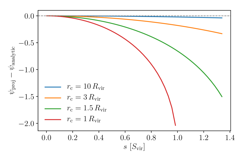
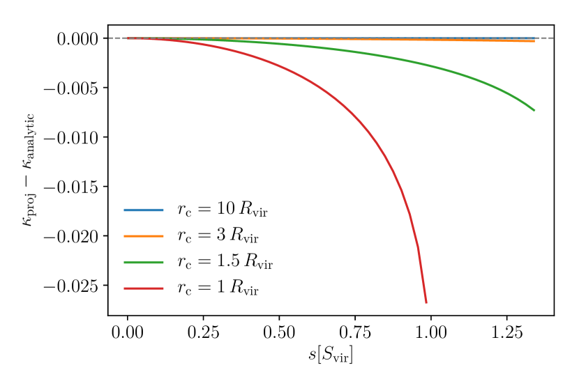
The applicability of this approximation critically depends on . For large enough fields of view, the gravitational potential may drop to sufficiently small absolute values within such that the unaccounted region does not significantly contribute to the integral and therefore can safely be neglected. However, if the field of view is comparable to the virial radius of the cluster, these neglected contributions become increasingly important and simply cutting them away introduces artefacts that severely alter the radial curvature of the resulting lensing potential and systematically bias conclusions on the mass distribution of the lens. Figure 1(a) illustrates this effect. It shows the difference between the projected potential of a Navarro-Frenk-White (NFW) halo (Eq. (24)) and the analytical lensing potential. If the integral is truncated at the virial radius, the result significantly deviates from the truth for all radii. With increasing truncation radius, the differences become smaller and are restricted to increasingly large radii. This effect is less pronounced for functions that fall off more steeply, as can be seen in Fig. 1(b) where the same procedure is shown for half the projected density compared to the analytically known convergence. Since the X-ray emissivity of the ICM is quadratic in the gas density and therefore falls off even more steeply, it is not surprising that truncation artefacts usually do not interfere with the RL deprojection algorithm even though it includes a reprojection in every iteration.
2.4.2 Analytic continuation
To mitigate these artefacts, we chose to introduce an analytic continuation of the 3D gravitational potential outside of . Several functional forms are possible. For this work we chose
| (25) |
where and are fixed by continuity conditions. The implied underlying assumption is that there is no significant mass contribution outside of and that therefore the potential in this radial range is dominated by the mass enclosed within . While this assumption most likely does not hold in a strict sense, tests with hydrodynamical simulations show that it is sufficient to reconcile reconstructed and true projected potential (see Section 4.2). The modified projection integral then reads
| (26) |
where is an upper bound for the continuation, which needs to be introduced as most reasonable functional forms still formally diverge when integrated up to infinite radius.
2.5 Sanity checks
As mentioned above, the parameters of the analytic continuation are set by continuity conditions, i.e. by demanding that the values of and its first derivative coincide with the respective values in the deprojected profile. In order to ensure that especially the radial derivative for the latter is still driven by data rather than noise at we employ a series of simple sanity checks.
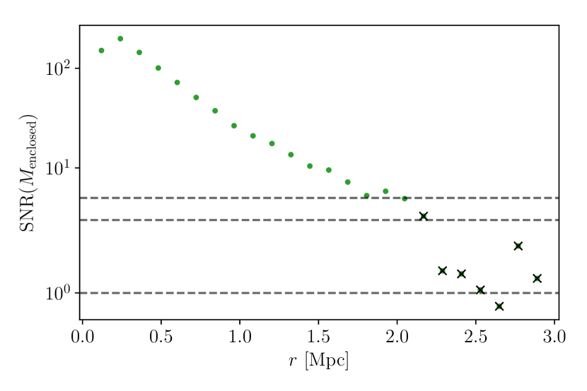
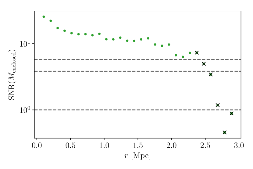
We estimate the signal-to-noise ratio for the enclosed mass as a function of radius
| (27) |
from Poisson realisations of the X-ray data as this directly sets the slope of the continuation . Figure 2 shows an example for the mock NFW halo in Section 4.1. Additionally we check for unphysical behaviour by testing the non-negativity of the Laplacian , which is proportional to the density via Poisson’s equation.
If the outer bins fail to meet these criteria, the analytic continuation parameters would likely be set by random fluctuations and introduce new artefacts rather than correcting those induced by truncating the projection integral. Therefore, if necessary we cut the profile at the outermost radial bin where both conditions are still satisfied and start the continuation there.
3 Joint reconstruction framework
3.1 SaWLens2 in a nutshell
SaWLens2 is a modular C++ code framework for free-form and mesh-free reconstructions of projected gravitational potentials from observational data. Its core idea, to use a regularised maximum-likelihood estimator to reconstruct the lensing potential without relying on a specific mass model, was first presented in Bartelmann et al. (1996). The maximum posterior reconstruction is found by directly solving the linear system of equations obtained from minimising the log-likelihood, which is done iteratively as necessitated by the non-linear dependence of some observables on the projected potential. Previous implementations, based on adaptively refined but regular grid layouts as reconstruction domains, have been successfully applied to clusters in the CLASH sample (Postman et al., 2012; Merten et al., 2015). The latest mesh-free implementation based on strong and weak lensing constraints is described in detail in Merten (2016). We briefly summarise the main ideas here before focusing on ways to augment this framework with constraints from the ICM.
3.2 Mesh-free support
SaWLens2 reconstructs the projected gravitational potential on a set of support nodes, which are not required to fulfil any sort of regularity or aspect ratio criteria. Thus, the reconstruction domain can easily be adapted to data sets that are distributed non-uniformly and on very different spacial scales, allowing for intuitive mask treatment and the combination of distinct data sets (e.g. a catalogue of weakly lensed background galaxies spanning several arc minutes with a set of strongly lensed multiple images only separated by tens of arc seconds). The obvious challenge is that interpolation and finite differencing schemes, which are required in free-form lens reconstructions, become less straightforward. Here, we make use of radial basis functions (RBF), a set of radially dependent functions centred on the nodes that make up the mesh-free domain. By expanding fields on the mesh-free domain in terms of these analytical RBFs, we can interpolate these fields to a different set of support nodes and define finite differencing stencils to obtain numerical derivatives. For a detailed description of RBFs, mesh-free domains, and their application to lens reconstructions, see Merten (2016), Fornberg et al. (2011) and Fornberg et al. (2013) and references therein. The handling of mesh-free domains, including interpolations and finite differences, is implemented in a publicly available C++ library111https://bitbucket.org/jmerten82/libmfree.
3.3 Lensing
Equation (6), restricted to the case of , sets the way shear measurements are incorporated in a SaWLens2 reconstruction. After defining a set of reconstruction nodes, here chosen to be a subsample of sheared galaxy positions, ellipticities of galaxies in the vicinity of each node are averaged to obtain an estimate of . This averaging process introduces covariances when neighbouring nodes have overlapping galaxy samples. This, together with shape noise, is captured in the covariance matrix (for details on its calculation see Merten, 2016). The log-likelihood to be maximised by the reconstructed lensing potential then reads
| (28) |
where is the appropriate finite differencing operator for the respective component of the complex shear. We note that in order to maintain linearity in , the value of is based on a prior and iteratively updated (see also Section 3.5).
3.4 Including X-ray data
Several ways to include a potential estimate based on de- and reprojected X-ray data are conceivable, depending on the specific RL implementation and data available. In general, the respective log-likelihood term that enters the SaWLens2 reconstruction will be of the form
| (29) |
Here denotes any operator that ensures compatibility of the coordinate basis of the model and that of the data-based , and denotes the covariance matrix of . If non-spherical symmetry assumptions (e.g. ellipsoidal) were used in the RL step, and thus were given for a grid with the resolution of the X-ray detectors CCD, would be designed to assign the reconstruction nodes of the mesh-free support to the corresponding pixels of .
In the present case of spherical symmetry, is given as a radial profile obtained from azimuthally averaged X-ray surface brightness observations, and thus in this case is designed as a azimuthal averaging operator. It takes the form of an -matrix, where is the number of radial bins for , and is the number of reconstruction nodes used. It has elements
| (30) |
where is the number of nodes that lie within the radial bin . This way, the log-likelihood in Eq. (29) ensures that the reconstructed potential values on (azimuthal) average follow the profile while still leaving enough freedom for local deviations from spherical symmetry required by lensing constraints, for example due to significant substructure or an overall non-spherical cluster morphology.
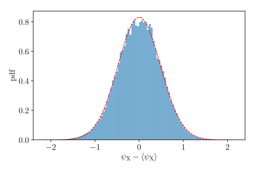
In order to get an estimate of we create Poisson realisations of the observed photon count maps and subject them to the de- and reprojection process to arrive at realisations of the X-ray-based lensing potential, from which we can compute the corresponding covariance. We further use these realisations of the estimated potential to test if a Gaussian likelihood is applicable at all, and use the mean profile (which by construction is identical to the one based on the original data) in Eq. (29).
3.5 Regularisation
Regularisation is required in a free-form framework to avoid overfitting. We adopt a two-level iteration scheme as described in Bradač et al. (2005), Merten et al. (2009) and Merten (2016). Starting with a low number of initial support nodes allows us to average over a comparably large number of neighbouring galaxies and hence significantly reduces shape noise. Subsequently increasing the number of nodes and reducing the number of galaxies in the averaging samples increases resolution and allows to resolve smaller structures. On each resolution level we iteratively solve for while regularising on a moving prior in convergence and shear
| (31) | |||||
| (32) |
where is the finite differencing operator for (half) the 2D Laplacian and the diagonal matrices set the regularisation strength. With increasing resolution the result of the coarser gets interpolated to the finer domain and poses as the initial regularisation prior.
3.6 Error estimation and goodness of fit
We analyse the normalised residuals to assess the quality of our reconstruction. To this end we transform the residual vector
| (33) |
for the combined data set and the corresponding combined response into the eigenbasis of the combined inverse data covariance, in which the latter is diagonal, i.e.
| (34) |
Here is the total number of data points, are the eigenvalues of the combined inverse data covariance, and is the corresponding basis change operator. The normalised residuals are then
| (35) |
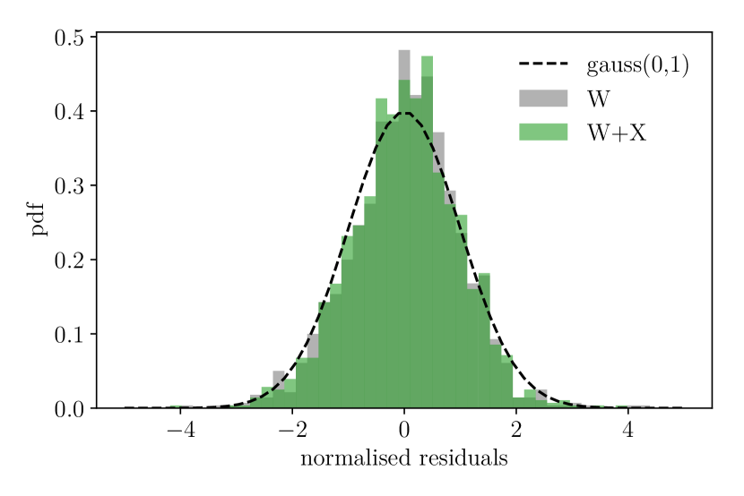
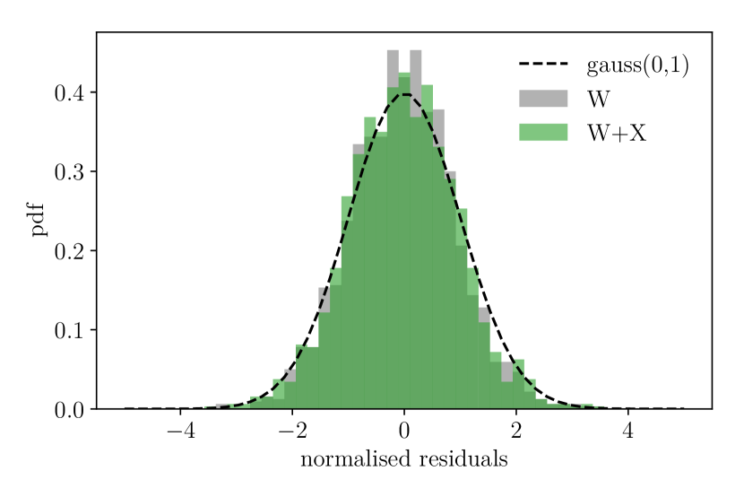
which should follow a Gaussian distribution with zero mean and standard deviation , if all errors have been taken into account and regularisation has been chosen properly.
We employ re-sampling to estimate the uncertainties for the final reconstruction. We create a number of bootstrapped realisations of the shear catalogue and also bootstrap the X-ray-based lensing potential profile, by resampling the Poisson realisations created for the covariance estimation and averaging over the resampled set instead of the original to create the mean projected profile, but keeping the original covariance matrix. The set of reconstructions obtained from these bootstrapped inputs is interpolated to the mesh-free domain of the default reconstruction and used to estimate the standard deviation of reconstructed quantities node by node. 222A small fraction of bootstrap realisations returns entirely unphysical results (e.g. convergence values orders of magnitudes above the weak lensing regime) due to numerical instabilities. We discard the obviously corrupted cases before performing the error estimation.
4 Testing the method
4.1 Mock NFW
First we consider a simple cluster model where all assumptions are true by construction: a NFW halo with a polytropic ICM in hydrostatic equilibrium. We set the virial mass of the halo to at redshift , assuming the concentration-mass-relation from Seljak (2000) and Klypin et al. (2001). The lensing properties of NFW halos are analytically known (e.g. Golse & Kneib, 2002), so we could easily create a mock shear catalogue of roughly randomly distributed galaxies, where we added Gaussian shape noise with . We followed the formalism of Komatsu & Seljak (2001) to model the ICM in hydrostatic equilibrium with a polytropic stratification with index . We created a surface brightness map with the same field of view as the shear catalogue and assumed a mean photon energy of , an exposure time of and a detector with an effective area of . All defining properties of the halo and the mock observations are summarised in Table 1.
| Halo | Lensing | X-ray |
|---|---|---|
| FoV | FoV | |
We added Poisson noise to the resulting X-ray surface brightness before creating Poisson realisations of the surface brightness profile in linearly spaced radial bins. We deprojected these realisations with the RL algorithm to determine the Newtonian potential profile, using the correct polytropic index and temperature of .
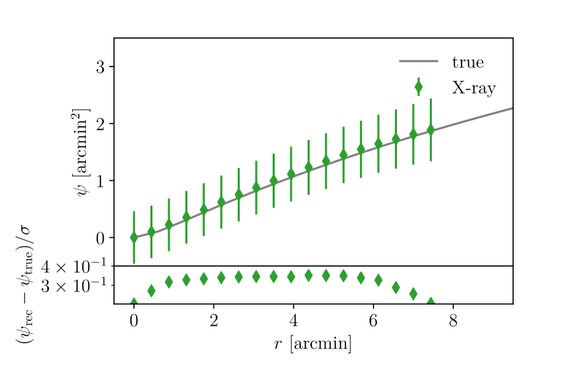
Based on the realisations of , we estimated the signal-to-noise ratio of the enclosed mass as a function of radius, as discussed in Section 2.5 and depicted in Fig. 2. We also computed the Laplacian of the potential as a proxy for the total density. We discarded all bins that fail our checks, i.e. where the Laplacian is negative or where the signal-to-noise ratio falls below . The thus truncated potential profile was subsequently projected along the line of sight, using the analytic continuation according to Section 2.4 up to a cut-off radius of three times the truncated data radius. The reconstructed lensing potential profile is compared to the true profile in Fig. 3. The error bars depict the standard deviation within the sample of realisations, and their large size in comparison to the scatter in the data points in part reflects the high degree of correlation between bins.
Even without knowing the true lensing potential, an appropriate cut-off radius for the analytical continuation can be found by gradually increasing it from the truncated data radius. If the cut-off radius is too small, the projection artefacts manifest themselves in deviations in the radial curvature of the potential at increasing radii (with increasing cut-off, see Fig. 1(a)). These curvature deviations lead to ring-like artefacts on the reconstructed convergence map. This of course does not pin down the proper cut-off radius entirely, but gives a lower limit.
The realisations of are Gaussian distributed and we scale all realisations to a reference redshift of and use them to compute the inverse covariance matrix of the projected potential profile.
With in place, we ran SaWLens2, once using the shear data alone and once using both shear data and X-ray data. In both cases the mesh-free support was defined by subsampling the shear catalogues’ galaxy positions. We chose three resolution levels, with , , and nodes, leading to a final resolution of roughly per node. All parameters of the reconstruction are collected in Table 2. The normalised residuals, as discussed in Section 3.6, as well as further diagnostics of this and the following test case are presented in Appendix A.
| Nodes (nominal) | |||
| Nearest neighbours | |||
| Regularisation strength |
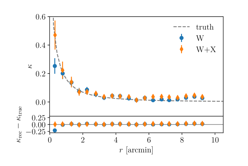
We ran 500 bootstrap realisations of the mock data, as described in Section 3.6, to estimate errors on the resulting convergence maps. Figure 4 shows the radial convergence profiles of the default reconstructions with error bars based on these realisations. Figures 5(a) and 5(b) depict the convergence maps and residuals for the shear-only (W from here on) and combined (WX) cases, respectively.
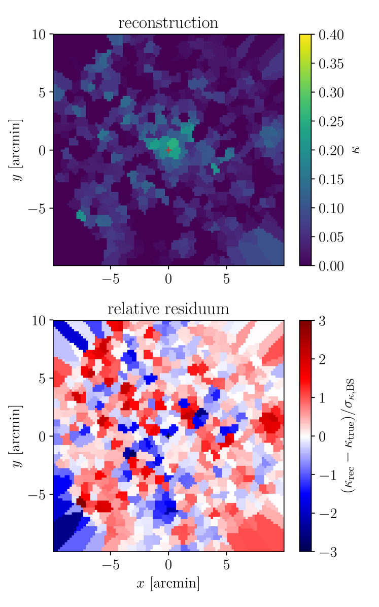
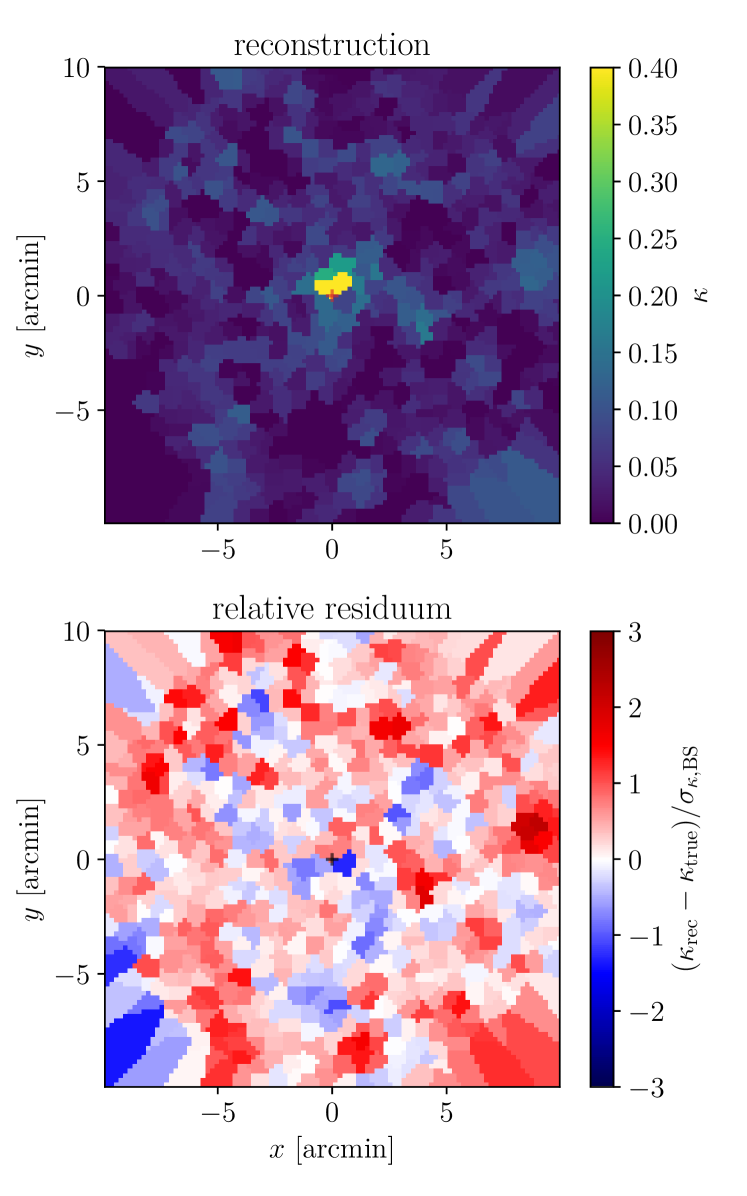
We find the following:
-
•
The correct amplitude of the central convergence peak is only recovered in the combined reconstruction, but not in the shear-only reconstruction;
-
•
The bootstrap-based error estimates for both cases are similar;
-
•
The error estimates increase towards the central peak, where picking a slightly different node position has the largest effect due to a large convergence gradient;
-
•
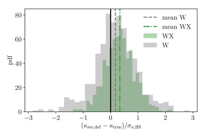
The residua relative to the bootstrap error, , show better agreement in the combined case, where they indicate a fairly unbiased reconstruction (i.e. the mean of the relative residua approximately vanishes).
4.2 Hydrodynamical simulation
To investigate the performance of the reconstruction framework when confronted with more realistic cluster morphologies and physics, we turn to a full hydrodynamical simulation of a cluster embedded in the cosmic web. We selected a massive cluster from Box2b/hr of the Magneticum333http://www.magneticum.org/ simulation suite (Dolag & Magneticum Core Team, in prep.; Hirschmann et al., 2014) through the public web interface444https://c2papcosmosim.uc.lrz.de first presented in Ragagnin et al. (2017). The simulations, and our subsequent treatment, adopt a WMAP7 cosmology (Komatsu et al., 2011). Box2b/hr follows particles in a volume of with the -body/SPH code P-Gadget3 (Springel, 2005; Beck et al., 2016) also incorporating non-gravitational effects such as radiative cooling, heating, star formation, and AGN feedback.
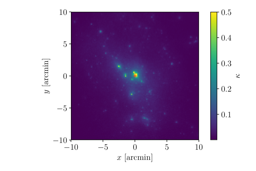
We selected a cluster with mass555 is the mass enclosed in a spherical region where the mean density is 500 times the background density. at redshift . Its convergence map is shown in Fig. 6. Table 3 lists some of its properties. We selected this particular cluster because it displays a structured and non-spherical morphology while being among the more massive halos in the box, providing sufficient signal-to-noise in the mock lensing and X-ray observations.
| Halo | Lensing |
|---|---|
| FoV | |
We employed PHOX (Biffi et al., 2012) and SIXTE666http://www.sternwarte.uni-erlangen.de/research/sixte/ (Schmid et al., 2010), both available in the interface, to generate synthetic X-ray observations of exposure with XMM-Newton’s EPIC-pn instrument. We used SMAC (Dolag et al., 2005), to obtain a total surface density map, from which we computed a convergence map and then a shear via the relation
| (36) |
with the convolution kernel
| (37) |
We then generated a map of the reduced shear and sampled it at a source density of to generate a catalogue of weakly lensed sources at redshift , adding again Gaussian shape noise with .
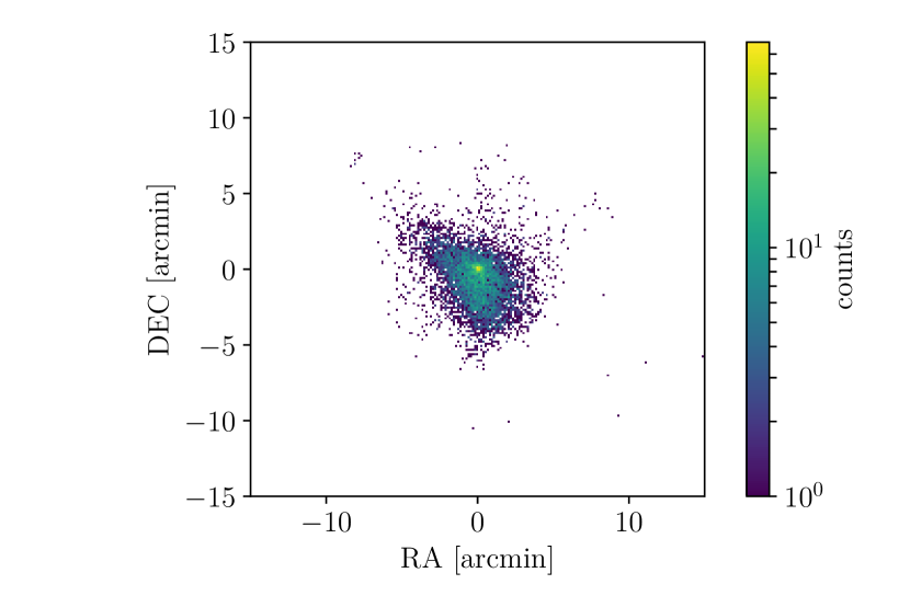
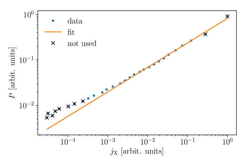
We also created a map of the thermal SZ Compton- signal of the cluster to estimate the polytropic index and a map of the ICM temperature to estimate the sound speed. For this we plot the electron pressure obtained from deprojecting the Compton- profile against the X-ray emissivity. If the assumptions discussed in Section 2.3 hold, both are related by
| (38) |
Figure 8 shows the pressure versus the emissivity together with a fit based on Eq. (38), excluding regions where the simple power law relation seems broken and the assumptions likely do not hold. The best fitting polytropic index is .
As in the previous example, we created Poisson realisations of the count profile777The radial bin size is chosen well above the PSF of the X-ray instrument., which were deprojected, converted to realisations of the Newtonian potential, and subjected to the same sanity checks. The results of these checks and further diagnostic plots can be found in Appendix A. The potential profiles were then projected, employing the analytic continuation scheme up to a radius of four times the truncated data radius. The resulting realisations were used to estimate the corresponding inverse covariance matrix.
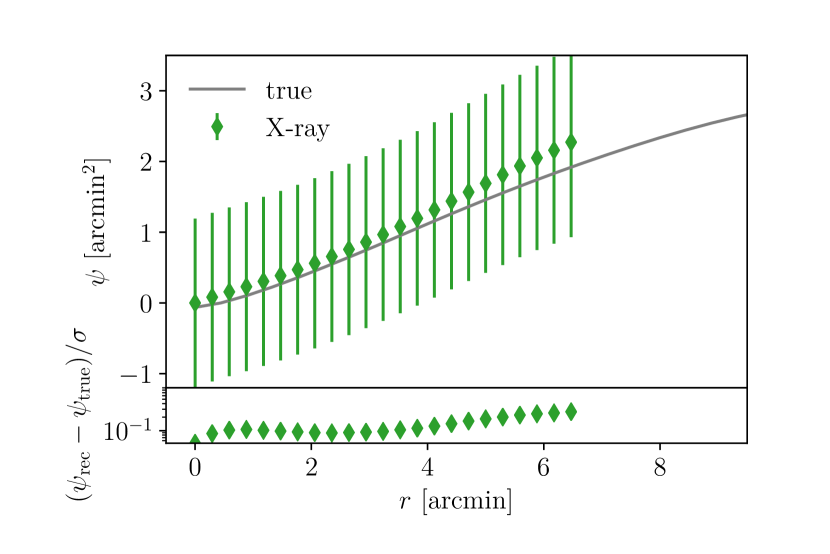
The mean lensing potential profile obtained from the X-ray data is compared to the actual lensing potential of the simulated cluster in Fig. 9. The curves agree well up to a radius of roughly arcmin where the X-ray-based estimate starts to deviate, but still well within the error margins. We chose the cut-off radius based on ballpark estimates of the virial radius from the surface brightness data and experience from Section 2.4. The error bars in Fig. 9 are noticeably larger than in the NFW case above. One reason for this is the choice of cut-off radius. The further out the extrapolation is taken, the more noisy features, even in the truncated potential profile, influence the continuation and thus the projection and consequently the variance throughout the realisations increases. A balance between extrapolating far enough to counter artefacts while still maintaining constraining power is required. So far rough estimates have proven to work sufficiently well.
| Nodes (nominal) | |||
| Nearest neighbours | |||
| Regularisation strength |
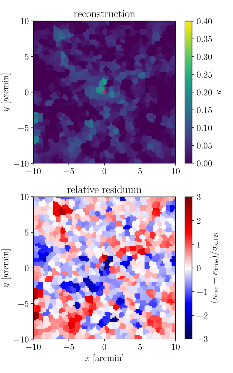
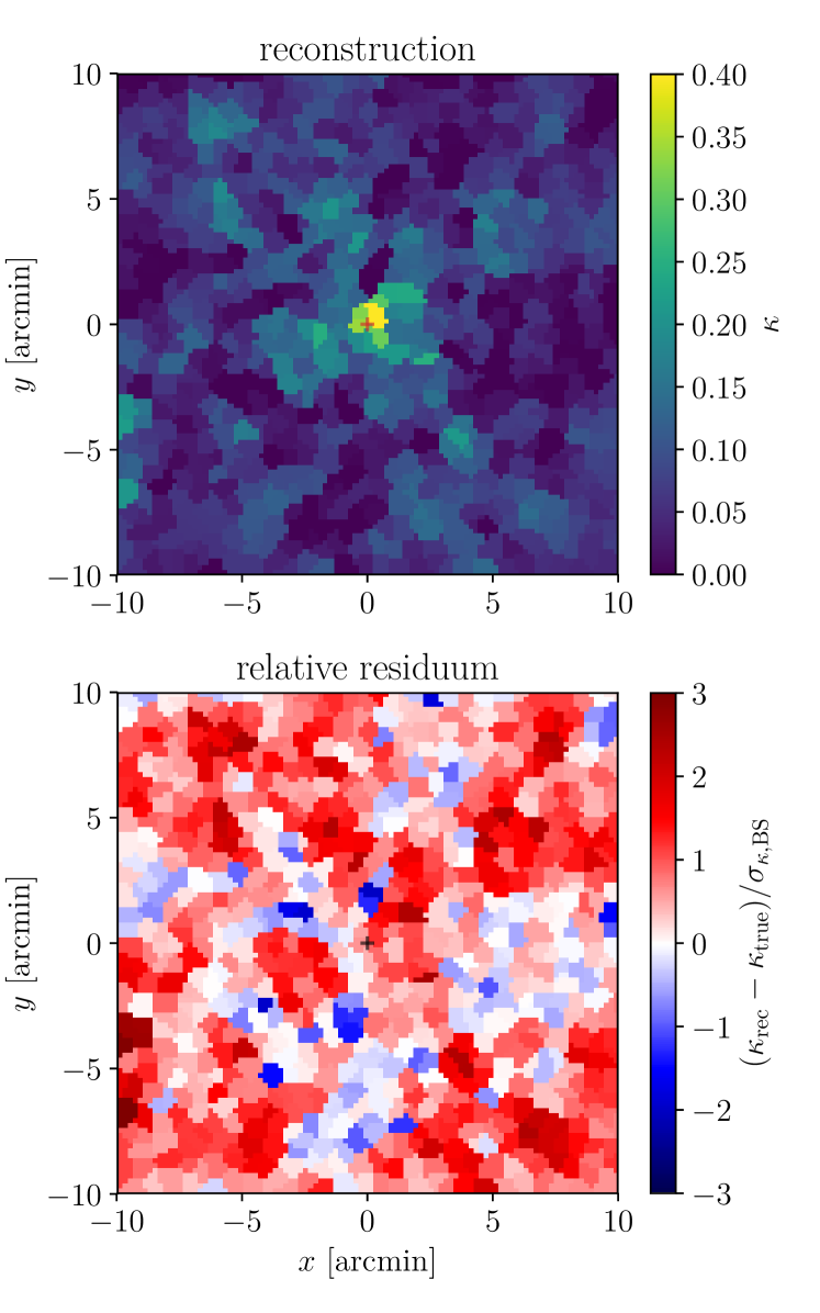
The following SaWLens2 reconstructions, as well as 500 bootstraps, were set up using the parameters collected in Table 4. Again, we performed one reconstruction using the shear catalogue alone and one combining shear and X-ray data. Figure 10 shows the convergence profiles with errors based on the bootstraps. The resulting convergence maps together with their relative residua based on bootstrapping are shown in Figs. 11(a) and 11(b).
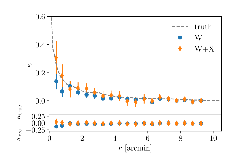
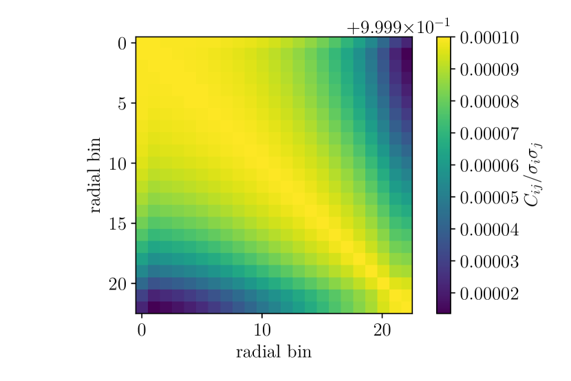
As in the previous use case, the combined reconstruction yields a more pronounced central convergence peak where the radial convergence profile nicely traces the true convergence, especially in the bootstrapped mean. We note, however, that the combined reconstruction is biased high in convergence, as can be seen in the relative residuum map in the lower plot of Fig. 11(b). Experiments with different cut-off radii in the projection step for the X-ray constraint show that the bias is not related to deviations in the projected potential curvature alone. The scaling of the lensing potential is well reproduced (see Fig. 9), and the combination of shear- and X-ray-based constraints in SaWLens2 does not generally introduce a significant bias in the reconstructed convergence (see previous section). Further investigation reveals that this bias originates in the combination of two factors. The recovered profile of the lensing potential based on X-ray data deviates slightly from the truth (see Fig. 9), and the covariance matrix is very dense, effectively correlating every radial bin with every other, as can be seen from the Pearson correlation matrix depicted in Fig. 19. This way, slight overestimations of the radial curvature in the outer bins lead to slight additive biases in the convergence of the joint reconstruction. The radial profiles in Fig. 10 are adjusted for this bias.
In order to quantify how the reconstruction deals with the pronounced triaxial morphology of the cluster, we calculated the second moment tensor
| (39) |
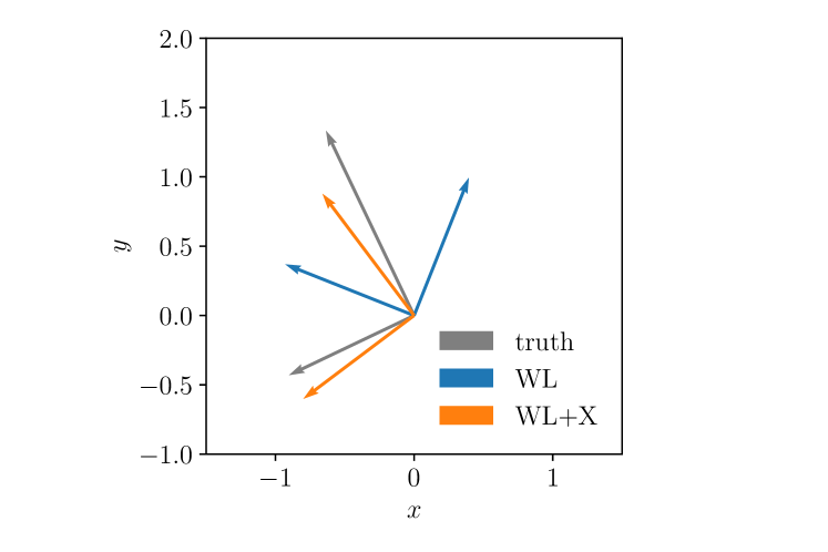
for the convergence map, where the sum runs over all nodes in the reconstruction, and the Heaviside function ensures that only nodes with convergence above a certain threshold are taken into consideration. The eigenvectors of this tensor align with the major axes of the halo, while the ratio of its eigenvalues reflects the square of the ratio of the major axes.
The corresponding eigenvectors are shown in Fig. 12, scaled to reflect the reconstructed eigenvalue ratio. The X-ray-based information does not add information on the morphology (as it is based on spherical symmetry to create an estimate of the radial profile of the lensing potential), but since the reconstruction is only required to follow this profile on azimuthal average, it also does not impose any morphology. In cases where the noise in the reconstruction is reduced by the addition of X-ray data, the constraints on the morphology may be improved. In the present case, where we used the median reconstructed convergence as a threshold for Eq. (39), the reconstructions only poorly reflect the axis ratio of the true map, but the combined reconstruction matches the directions of the major axes significantly better than in the shear-only case.
This is not a particularly stable result. Changes in the iteration and regularisation settings may alter the inferred second-moment tensor without significantly changing the normalised data residuals or other reconstruction results. It therefore remains doubtful if the addition of symmetrised X-ray constraints can improve the inference of the morphology of a real cluster. We expect, however, that X-ray constraints using deprojections with spheroidal symmetry are bound to improve this measure; Fig. 7 shows a clear elongation of the surface brightness, paralleling that of the underlying mass distribution.
5 Conclusions
5.1 Summary
In this work we demonstrated how to jointly incorporate weak lensing and X-ray data in a mesh-free free-form reconstruction framework in order to infer the surface mass distribution of a galaxy cluster. We reviewed how the Richardson-Lucy algorithm can be used to deproject the X-ray surface brightness of the ICM and how the resulting emissivity can be connected to the Newtonian potential. We discussed numerical artefacts in the projected potential that may arise when the usable data range of X-ray observations is approximately the same as or narrower than that of the virial radius, and we present means to compensate these artefacts. We presented the current implementation of the reconstruction framework, SaWLens2, and how X-ray constraints that have been symmetrised during the de- and reprojection steps can be included without imposing any symmetry on the joint reconstruction. Subsequently, we tested the method on two mock clusters, one a simple NFW halo in hydrostatic equilibrium and one a realistic cluster taken from a cosmological hydrodynamical simulation. These tests showed that the addition of X-ray information can significantly improve the reconstruction, especially in the central region, where the peak in convergence can be recovered much better than in the shear-only case. Quantitatively, the reconstruction based on shear alone underestimates the true radial convergence profile in the central region by or roughly a factor of , whereas the combined reconstruction traces the true convergence almost perfectly down to a projected radius of around arcmin, with a residuum of only . The combined reconstruction for a realistic cluster displayed a small bias (, see Appendix A) towards higher convergence values. This effect is due to the high degree of correlation between radial bins in the X-ray-based potential estimate and slight deviations in the outer bins. Since this is a purely additive bias in the convergence, it is mitigated relatively easily. This highlights once more the need for the careful treatment of artefacts in the projection step as they can alter the results across the whole domain.
5.2 Scope and possible extensions
It is worthwhile to also explicitly summarise the limiting and simplifying assumptions that went into our reconstruction method, and how it might be generalised.
We assume that the CDM framework is an adequate description of the Universe.
In the context of gravitational lensing, we limit ourselves to cases that can be sufficiently described in the single thin lens approximation and assume that intrinsic alignment is a negligible source of systematic error on scales relevant for cluster lensing. More involved lensing scenarios, where intrinsic alignment is taken into account can be implemented by altering the computation of the shear covariance matrix.
In the context of using X-ray data as an additional constraint, we assume that the ICM
is in hydrostatic equilibrium. This is needed to connect the gas structure to the total Newtonian potential. However, corrections for hydrostatic bias (e.g. Shi, 2016) can be incorporated. We further assume the ICM to be describable as an ideal gas that is polytropically stratified over a significant radial range.
The systematic effects on the reconstructed potential due to these assumptions are currently investigated and will be described in an upcoming paper (Tchernin et al. in prep).
Specifically, the combination of lensing and non-lensing constraints as presented here only works if general relativity is the assumed theory of gravity as otherwise lensing and the ICM density probe different combinations of the Bardeen potentials, which are
in general not identical (Bardeen, 1980).
Parametrised deviations from general relativity (e.g. Zhao et al., 2009) can in principle be incorporated to either allow a consistent reconstruction assuming modified gravity or to test for such deviations.
Since the approach presented here for X-ray observations, can also be applied to measurements of the thermal SZ signal and member galaxy kinematics, and since strong lensing features are readily included, a joint analysis has the potential to constrain the mass distribution across all scales accessible to observations.
There are several sources of arbitrariness in the method as presented here, namely the values of hyper-parameters like the regularisation strength and the specifics of the iteration and shear averaging scheme, as well as the choice of cut-off radius in the analytic continuation. While there are reasonable experience-based guidelines for choosing these parameters, there is still considerable leeway and the result may be affected by that, without significantly altering the measures of goodness of fit.
As our test on simulated data show, the presented way of combining weak lensing and X-ray data relies on relatively high spatial resolution for the two data sets. Future applications to real data are therefore likely pointed observations of individual massive clusters rather than statistical samples from survey data. For the former, the tools and methods presented here may allow a free-form assessment of cluster morphology across a wide range of scales, thus potentially informing statistically more precise methods, for example in the modelling of clusters as strong lenses. However, applications to real data are also likely complicated by several factors. For instance noisy measurements of ICM temperature as well as correlated and/or non-Poissonian noise in the X-ray surface brightness measurements may affect subsequent estimates of the gravitational potential.
Acknowledgements.
KH thanks Kerstin Paech and Steffen Hagstotz for many helpful discussions. KH and SH acknowledge the support of the DFG cluster of excellence ‘Origin and Structure of the Universe’ (www.universe-cluster.de). JM acknowledges funding from the European Union’s Horizon 2020 research and innovation programme under the Marie Skłodowska-Curie grant agreement No. 664931. CT acknowledges the support of the Deutsche Forschungsgemeinschaft under BA 1369 / 28-1 and of the Swiss National Science Foundation under P2GEP2 159139. Parts of this work were performed using the libastro code library developed by the cosmology group at ITA Heidelberg.References
- Allen et al. (2011) Allen, S. W., Evrard, A. E., & Mantz, A. B. 2011, Annual Review of Astronomy and Astrophysics, 49, 409
- Angrick & Bartelmann (2009) Angrick, C. & Bartelmann, M. 2009, Astronomy and Astrophysics, 494, 461
- Angrick & Bartelmann (2012) Angrick, C. & Bartelmann, M. 2012, Astronomy and Astrophysics, 538, A98
- Angrick et al. (2015) Angrick, C., Pace, F., Bartelmann, M., & Roncarelli, M. 2015, Monthly Notices of the Royal Astronomical Society, 454, 1687
- Bardeen (1980) Bardeen, J. M. 1980, Physical Review D, 22, 1882
- Bartelmann (2010) Bartelmann, M. 2010, Classical and Quantum Gravity, 27, 233001
- Bartelmann et al. (1996) Bartelmann, M., Narayan, R., Seitz, S., & Schneider, P. 1996, The Astrophysical Journal Letters, 464, L115
- Beck et al. (2016) Beck, A. M., Murante, G., Arth, A., et al. 2016, Monthly Notices of the Royal Astronomical Society, 455, 2110
- Biffi et al. (2016) Biffi, V., Borgani, S., Murante, G., et al. 2016, The Astrophysical Journal, 827, 112
- Biffi et al. (2012) Biffi, V., Dolag, K., Böhringer, H., & Lemson, G. 2012, Monthly Notices of the Royal Astronomical Society, 420, 3545
- Bocquet et al. (2018) Bocquet, S., Dietrich, J. P., Schrabback, T., et al. 2018, arXiv e-prints, 1812, arXiv:1812.01679
- Bonamigo et al. (2018) Bonamigo, M., Grillo, C., Ettori, S., et al. 2018, ArXiv e-prints, 1807, arXiv:1807.10286
- Bradač et al. (2005) Bradač, M., Schneider, P., Lombardi, M., & Erben, T. 2005, Astronomy and Astrophysics, 437, 39
- Collaboration et al. (2016) Collaboration, P., Ade, P. a. R., Aghanim, N., et al. 2016, Astronomy and Astrophysics, 594, A24
- Diego et al. (2007) Diego, J. M., Tegmark, M., Protopapas, P., & Sandvik, H. B. 2007, Monthly Notices of the Royal Astronomical Society, 375, 958
- Dietrich et al. (2019) Dietrich, J. P., Bocquet, S., Schrabback, T., et al. 2019, Monthly Notices of the Royal Astronomical Society, 483, 2871
- Dolag et al. (2009) Dolag, K., Borgani, S., Murante, G., & Springel, V. 2009, Monthly Notices of the Royal Astronomical Society, 399, 497
- Dolag et al. (2005) Dolag, K., Hansen, F. K., Roncarelli, M., & Moscardini, L. 2005, Monthly Notices of the Royal Astronomical Society, 363, 29
- Dolag & Magneticum Core Team (in prep.) Dolag, K. & Magneticum Core Team. in prep.
- Fornberg et al. (2011) Fornberg, B., Larsson, E., & Flyer, N. 2011, SIAM Journal on Scientific Computing, 33, 869
- Fornberg et al. (2013) Fornberg, B., Lehto, E., & Powell, C. 2013, Computers & Mathematics with Applications, 65, 627
- Golse & Kneib (2002) Golse, G. & Kneib, J.-P. 2002, Astronomy and Astrophysics, 390, 821
- Hirschmann et al. (2014) Hirschmann, M., Dolag, K., Saro, A., et al. 2014, Monthly Notices of the Royal Astronomical Society, 442, 2304
- Jauzac et al. (2016) Jauzac, M., Eckert, D., Schwinn, J., et al. 2016, ArXiv e-prints, 1606, arXiv:1606.04527
- Klypin et al. (2001) Klypin, A., Kravtsov, A. V., Bullock, J. S., & Primack, J. R. 2001, The Astrophysical Journal, 554, 903
- Kneib et al. (2004) Kneib, J.-P., Ellis, R. S., Santos, M. R., & Richard, J. 2004, The Astrophysical Journal, 607, 697
- Komatsu & Seljak (2001) Komatsu, E. & Seljak, U. 2001, Monthly Notices of the Royal Astronomical Society, 327, 1353
- Komatsu et al. (2011) Komatsu, E., Smith, K. M., Dunkley, J., et al. 2011, The Astrophysical Journal Supplement Series, 192, 18
- Konrad et al. (2013) Konrad, S., Majer, C. L., Meyer, S., Sarli, E., & Bartelmann, M. 2013, Astronomy and Astrophysics, 553, A118
- Kravtsov & Borgani (2012) Kravtsov, A. V. & Borgani, S. 2012, Annual Review of Astronomy and Astrophysics, 50, 353
- Liesenborgs et al. (2010) Liesenborgs, J., de Rijcke, S., & Dejonghe, H. 2010, Astrophysics Source Code Library, 1011.021
- Lucy (1974) Lucy, L. B. 1974, The Astronomical Journal, 79, 745
- Lucy (1994) Lucy, L. B. 1994, Astron. Astrophys., 289, 983
- Majer et al. (2016) Majer, C. L., Meyer, S., Konrad, S., Sarli, E., & Bartelmann, M. 2016, Monthly Notices of the Royal Astronomical Society, 460, 844
- Mantz et al. (2016) Mantz, A. B., Allen, S. W., Morris, R. G., et al. 2016, Monthly Notices of the Royal Astronomical Society, 463, 3582
- Markevitch (1998) Markevitch, M. 1998, The Astrophysical Journal, 504, 27
- McClintock et al. (2019) McClintock, T., Varga, T. N., Gruen, D., et al. 2019, Monthly Notices of the Royal Astronomical Society, 482, 1352
- Merten (2016) Merten, J. 2016, Monthly Notices of the Royal Astronomical Society, 461, 2328
- Merten et al. (2009) Merten, J., Cacciato, M., Meneghetti, M., Mignone, C., & Bartelmann, M. 2009, Astronomy and Astrophysics, 500, 681
- Merten et al. (2011) Merten, J., Coe, D., Dupke, R., et al. 2011, Monthly Notices of the Royal Astronomical Society, 417, 333
- Merten et al. (2015) Merten, J., Meneghetti, M., Postman, M., et al. 2015, The Astrophysical Journal, 806, 4
- Morandi et al. (2012) Morandi, A., Limousin, M., Sayers, J., et al. 2012, Monthly Notices of the Royal Astronomical Society, 425, 2069
- Penna-Lima et al. (2017) Penna-Lima, M., Bartlett, J. G., Rozo, E., et al. 2017, Astronomy and Astrophysics, 604, A89
- Postman et al. (2012) Postman, M., Coe, D., Benítez, N., et al. 2012, The Astrophysical Journal Supplement Series, 199, 25
- Ragagnin et al. (2017) Ragagnin, A., Dolag, K., Biffi, V., et al. 2017, Astronomy and Computing, 20, 52
- Reblinsky (2000) Reblinsky, K. 2000, Astronomy and Astrophysics, v.364, p.377-390 (2000), 364, 377
- Sarli et al. (2014) Sarli, E., Meyer, S., Meneghetti, M., et al. 2014, Astron. Astrophys., 570, A9
- Schmid et al. (2010) Schmid, C., Martin, M., Wilms, J., et al. 2010, X-ray Astronomy 2009; Present Status, Multi-Wavelength Approach and Future Perspectives, 1248, 591
- Schneider & Seitz (1995) Schneider, P. & Seitz, C. 1995, Astronomy and Astrophysics, 294, 411
- Seljak (2000) Seljak, U. 2000, Monthly Notices of the Royal Astronomical Society, 318, 203
- Sereno et al. (2017) Sereno, M., Ettori, S., Meneghetti, M., et al. 2017, Monthly Notices of the Royal Astronomical Society, 467, 3801
- Shi (2016) Shi, X. 2016, ArXiv e-prints, 1603, arXiv:1603.01742
- Shi & Komatsu (2014) Shi, X. & Komatsu, E. 2014, Monthly Notices of the Royal Astronomical Society, 442, 521
- Sifón et al. (2013) Sifón, C., Menanteau, F., Hasselfield, M., et al. 2013, The Astrophysical Journal, 772, 25
- Springel (2005) Springel, V. 2005, Monthly Notices of the Royal Astronomical Society, 364, 1105
- Suyu et al. (2017) Suyu, S. H., Bonvin, V., Courbin, F., et al. 2017, Monthly Notices of the Royal Astronomical Society, 468, 2590
- Tchernin et al. (2018) Tchernin, C., Bartelmann, M., Huber, K., et al. 2018, Astronomy and Astrophysics, 614, A38
- Umetsu (2013) Umetsu, K. 2013, The Astrophysical Journal, 769, 13
- Zhao et al. (2009) Zhao, G.-B., Pogosian, L., Silvestri, A., & Zylberberg, J. 2009, Physical Review Letters, 103, 241301
Appendix A Further diagnostics
Figure 13 shows that the assumption of a Gaussian likelihood in Eq. (29) is justified when the noise in the X-ray data is Poissonian. We show results of the sanity checks described in Section 2.5 for the NFW halo in Fig. 2 and for the realistic cluster in Fig. 16, indicating how the recovered profile of the three-dimensional Newtonian potential is truncated before the analytical continuation is applied in the projection step. Histograms of the normalised residuals of the reconstruction are compared to the expected Gaussian of unit variance in Fig. 14 for the NFW halo and Fig. 17 for the realistic cluster and show relatively good agreement, indicating appropriately chosen regularisation.
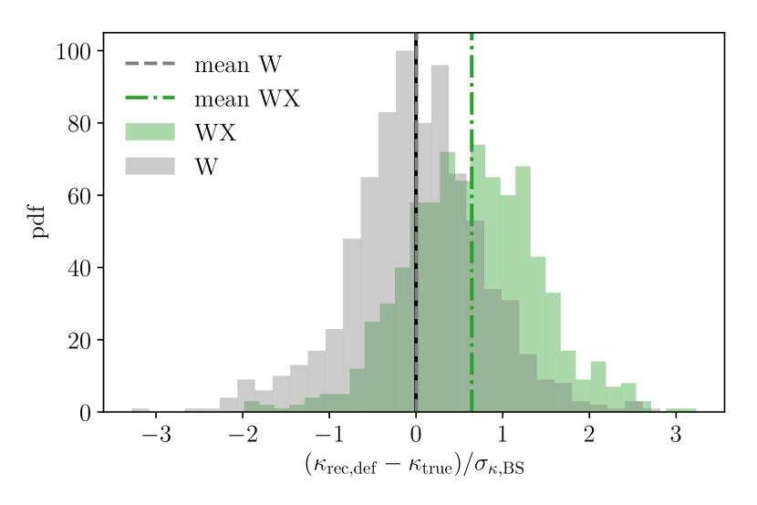
In Figs. 15 and 18, the histogram of the relative residuum of the reconstruction for the NFW mock and the realistic cluster respectively are shown. While the lensing-only reconstruction does not show any significant bias, the combined reconstruction of the realistic cluster is noticeably shifted towards higher convergence values by about .
Appendix B Minimising the X-ray log-likelihood
For the sake of completeness we explicitly show the contribution of the X-ray data to the LSE to be solved in SaWLens2. All other terms (lensing and regularisation) can be found in (Merten 2016) and references therein.