Infrared features of gravitational scattering
and radiation in the eikonal approach

Marcello Ciafaloni

Dipartimento di Fisica, Università di Firenze
Via Sansone 1, 50019 Sesto Fiorentino, Italy
Dimitri Colferai

Dipartimento di Fisica, Università di Firenze and INFN, Sezione di Firenze
Via Sansone 1, 50019 Sesto Fiorentino, Italy

and

Gabriele Veneziano

Theory Department, CERN, CH-1211 Geneva 23, Switzerland
Collège de France, 11 place M. Berthelot, 75005 Paris, France

Following a semi-classical eikonal approach — justified at transplanckian energies order by order in the deflection angle $\Theta_{s}\sim\frac{4G\sqrt{s}}{b}\equiv\frac{2R}{b}$ — we investigate the infrared features of gravitational scattering and radiation in four space-time dimensions, and we illustrate the factorization and cancellation of the infinite Coulomb phase for scattering and the eikonal resummation for radiation. As a consequence, both the eikonal phase $2\delta(E,b)$ and the gravitational-wave (GW) spectrum $\frac{\mathrm{d}E^{\mathrm{GW}}}{\mathrm{d}\omega}$ are free from infrared problems in a frequency region extending from zero to (and possibly beyond) $\omega=1/R$. The infrared-singular behavior of $4$-D gravity leaves a memory in the deep infrared region ($\omega R\ll\omega b<1$) of the spectrum. At $\mathcal{O}\left(\omega b\right)$ we confirm the presence of logarithmic enhancements of the form already pointed out by Sen and collaborators on the basis of non leading corrections to soft-graviton theorems. These, however, do not contribute to the unpolarized and/or azimuthally-averaged flux. At $\mathcal{O}\left(\omega^{2}b^{2}\right)$ we find instead a positive logarithmically-enhanced correction to the total flux implying an unexpected maximum of its spectrum at $\omega b\sim 0.5$. At higher orders we find subleading enhanced contributions as well, which can be resummed, and have the interpretation of a finite rescattering Coulomb phase of emitted gravitons.

Preprint: CERN-TH-2018-268

1 Introduction

The recent discovery of gravitational waves (GW) in black-hole and neutron-star mergers [1, 2] has also revived interest in gravitational phenomena at the level of elementary-particle processes. It has also been argued [3] that progress in the latter domain would provide useful inputs on the determination of parameters that enter the effective-one-body (EOB) approach [4, 5] to GW emission from coalescing binary systems.

In particle physics, gravitational scattering of light particles or strings at extremely high (i.e. transplanckian) energies has been considered since the late eighties [6, 7, 8, 9, 10] mainly as a thought-experiment aimed at testing quantum-gravity theories at very high energies, and/or short distance.

At such energies, $\sqrt{s}/2\equiv E>m_{P}\equiv\sqrt{\hbar/G}$, and we meet a regime in which the effective gravitational coupling ${\alpha_{G}}\equiv Gs/\hbar$ is large. Since such a coupling basically occurs as an overall factor in the effective action (in $\hbar$ units) this suggests the validity of a semiclassical approximation. This eikonal approach to high-energy gravitational scattering was developed further by Amati, Ciafaloni and Veneziano (ACV) [11, 14, 15, 16] in a series of papers by deriving, in particular, higher order corrections to the eikonal function.

Another emerging property of transplanckian gravitational scattering is a sort of “anti-scaling” law by which the higher the center-of-mass energy, the softer the characteristic energy of the final particles. This property has been seen both in the string-size-dominated regime [10, 17] and in the bremsstrahlung process, both classically [18, 19] and at the quantum level [20, 21, 22, 23, 24]. It is basically related to the fact that multiplicities of final quanta grow like ${\alpha_{G}}$ i.e. with two powers of the center of mass energy. Of course such a feature fits extremely well with the well known behavior of the Hawking temperature [25] of a black-hole of gravitational radius $R\equiv 2G\sqrt{s}$, $T\sim\hbar/R\ll E$. Interestingly, such a softening of the final state already occurs in regimes (such as collision at large impact parameter $b\gg R$) that are not expected to lead to black hole formation. Our study of gravitational bremsstrahlung will concentrate therefore exclusively on the regime $\frac{\hbar\omega}{\sqrt{s}}\ll\frac{\hbar\omega}{m_{P}}\ll 1$. Note that this does not prevent considering a wide range of frequencies all the way from zero, to $1/b$, to $1/R$, or even higher.

More recently, the low-frequency gravitational bremsstrahlung spectrum has also been investigated [26, 27, 28] in connection with Weinberg’s soft-graviton theorem [29] and its extension to subleading orders [30, 31, 32, 33, 34, 35, 36, 37, 38, 39]. The possible emergence of large soft logarithms (in $D=4$) has been recently emphasized in [26, 27] as subleading contributions to soft theorems and a possible source of memory effects. This approach, unlike the eikonal one, is not limited to high energy or to small deflection angles, but only covers a tiny region of frequencies (basically the one below $1/b\ll 1/R$). Thus comparison of the two approaches is necessarily limited to the extreme lower end of the $\omega$ spectrum.

The purpose of the present paper is to illustrate the essentials of the eikonal model just mentioned, and then to focus on the derivation of soft-graviton features, in order to see whether they are affected by the $D=4$ infrared (IR) singularity of the gravitational interaction.

We should notice from start that, in our approach, we shall mostly refer to scattering at fixed impact parameter $b$, rather than fixed momentum transfer $Q$. In $b$-space the $S$-matrix exponentiates both the eikonal function $\delta(b,E)$, which controls time-delay and deflection angle, and the multi-graviton production amplitudes in the form of a coherent state immediately connected to classical GW radiation.

An important goal of the paper is to show (sec. 5) that the eikonal resummation — which is needed in order to cover sizeable deflection angles of order $\Theta_{E}\equiv 2R/b$ (the Einstein deflection angle) — is also able to build up divergence-free amplitudes. That is true both for scattering (due to the factorization in impact parameter space and to the cancellation [14] of the infinite Coulomb phase at that order) and for radiation (due to the smoothing out of the single-exchange amplitude by $s$-channel iteration).

Given such a regular behavior of the resumed amplitude, the study of soft limits is straightforward, and based on the simple form of the resummed radiation amplitude in the classical limit given in secs. 5, 6. At leading level, the energy emission spectrum — as already discussed in [18, 20, 21] — shows a $\log(1/\omega R)$ dependence in the intermediate-frequency region $1/b\ll\omega<1/R$, before saturating at the expected $\omega$-independent zero-frequency limit [40]. At subleading level, the rescattering Coulomb phase shows up in its finite and exponentiated form, generating a class of logs of relative order $[b\omega\log(1/b\omega)]^{n}$ in the $b\omega\ll 1$ limit, similar (if not identical) to those already proposed in [26, 27].

With the aim of being as much as possible self-contained the rest of the paper is organized as follows: In sec. 2 we recall some old results on the eikonal approximation to high energy elastic gravitational scattering. In sec. 3 we recall previous analysis of the single graviton emission amplitude and, in particular, our unified description of both the very soft (Weinberg) regime and not so soft (Lipatov) one. These results are then used in sec. 4 to recover in a simple way a previous result on the subleading correction to the eikonal phase and deflection angle. In sec. 5 we present the basic starting point for our study of soft gravitational bremsstrahlung in the form of an infrared-finite unitary $S$-matrix which agrees, in the appropriate limit, with the classical calculation obtained earlier by completely different techniques. Sec. 6 contains most of the new results of this work both on the sub-leading correction to circularly polarized spectra and on the sub-sub-leading positive, logarithmically enhanced, corrections to the ZFL in the frequency region $\omega b\ll 1$. We also show how this regime connects smoothly with a logarithmically decreasing one in the region $1/b<\omega<1/R$ leading to a peak in the flux around $\omega b\sim 0.5$ (and roughly independent of $R$). In sec. 7 we discuss our results and point to possible directions for future research.

2 Elastic eikonal scattering: a reminder

In this section we summarize the ideas and assumptions introduced in [21] in order to understand the main ingredients that our eikonal radiation picture is based upon.

Throughout this paper, as in [16], we will restrict our attention to collisions in 4-dimensional space-time and in the point-particle (or quantum field theory) limit. Consider the elastic gravitational scattering $p_{1}+p_{2}\to p^{\prime}_{1}+p^{\prime}_{2}$ of two ultrarelativistic particles, with external momenta parametrized as

$$p_{i}=E_{i}(1,{\boldsymbol{\Theta}}_{i},\sqrt{1-|{\boldsymbol{\Theta}}_{i}|^{2}})\,,$$ (2.1)

at center-of-mass energy $2E=\sqrt{s}\gg M_{P}$ and momentum transfer $Q^{\mu}\equiv p_{1}^{\prime\mu}-p_{1}^{\mu}=p_{2}^{\mu}-p_{2}^{\prime\mu}$ with transverse component ${\boldsymbol{Q}}=E{\boldsymbol{\Theta}}_{s}$; the 2-vectors ${\boldsymbol{\Theta}}_{i}=|{\boldsymbol{\Theta}}_{i}|(\cos\phi_{i},\sin\phi_{i})$ describe both azimuth $\phi_{i}$ and polar angles $|{\boldsymbol{\Theta}}_{i}|\ll 1$ of the corresponding 3-momentum with respect to the longitudinal $z$-axis.

This regime is characterized by a strong effective coupling $\alpha_{G}\equiv Gs/\hbar\gg 1$ and was argued by several authors [6, 8, 10, 14] to be described by an all-order leading approximation which has a semiclassical effective metric interpretation. The leading result for the $S$-matrix $S(b,E)$ in impact-parameter ${\boldsymbol{b}}$ space has the eikonal form

$$S(b,E)=\exp[2\mathrm{i}\delta_{0}(b,E)]\;,\qquad\delta_{0}(b,E)=\alpha_{G}\log\frac{L}{b}\;,\qquad b\equiv|{\boldsymbol{b}}|\;,$$ (2.2)

$L$ being a factorized — and thus unobservable — IR cutoff due to the infinite Coulomb phase [10].

Corrections to the leading form (2.2) involve additional powers of the Newton constant $G$ in two dimensionless combinations

$$\frac{\hbar G}{b^{2}}=\frac{l_{P}^{2}}{b^{2}}\;,\qquad\frac{4G^{2}s}{b^{2}}=\frac{R^{2}}{b^{2}}\sim\alpha_{G}\frac{l_{P}^{2}}{b^{2}}\gg\frac{l_{P}^{2}}{b^{2}}\,,$$ (2.3)

$l_{P}\equiv\sqrt{\hbar G}$ being the Planck length. Since $\alpha_{G}\gg 1$ we can neglect completely the first kind of corrections. Furthermore, we can consider the latter within a perturbative framework since the impact parameter $b$ is much larger than the gravitational radius $R\equiv 2G\sqrt{s}$.

In order to understand the scattering features implied by (2.2) we can compute the ${\boldsymbol{Q}}$-space amplitude

$$\frac{1}{s}M_{\mathrm{eik}}(s,{\boldsymbol{Q}}^{2})=4\int\mathrm{d}^{2}{\boldsymbol{b}}\;\mathrm{e}^{-\frac{\mathrm{i}{\boldsymbol{b}}\cdot{\boldsymbol{Q}}}{\hbar}}\frac{\mathrm{e}^{2\mathrm{i}\delta_{0}(b,E)}}{2\mathrm{i}}=\frac{8\pi\alpha_{G}}{{\boldsymbol{Q}}^{2}}\left(\frac{4\hbar^{2}}{{\boldsymbol{Q}}^{2}L^{2}}\right)^{-\mathrm{i}\alpha_{G}}\frac{\Gamma(1-\mathrm{i}\alpha_{G})}{\Gamma(1+\mathrm{i}\alpha_{G})}\;,$$ (2.4)

where the last expression is obtained strictly-speaking by extending the ${\boldsymbol{b}}$-integration up to small $|{\boldsymbol{b}}|\lesssim R$ [6], where corrections may be large. But it is soon realized that the ${\boldsymbol{b}}$-integration in (2.4) is dominated by the saddle-point

$${\boldsymbol{Q}}=E{\boldsymbol{\Theta}}_{s}({\boldsymbol{b}})=-E\frac{2R}{b}\hat{{\boldsymbol{b}}}=-2\alpha_{G}\frac{\hbar}{b}\hat{{\boldsymbol{b}}}\;,$$ (2.5)

which leads to the same expression for the amplitude, apart from an irrelevant ${\boldsymbol{Q}}$-independent phase factor. The saddle-point momentum transfer (2.5) comes from a large number $\langle n\rangle\sim\alpha_{G}$ of graviton exchanges (fig. 1), corresponding to single-hit momentum transfers $\langle|{\boldsymbol{q}}_{j}|\rangle\simeq\hbar/b$ which are small, with very small scattering angles $|{\boldsymbol{\theta}}_{j}|$ of order $\theta_{m}\simeq\hbar/(bE)$. The overall scattering angle — though small for $b\gg R$ — is much larger than $\theta_{m}$ and is $|{\boldsymbol{\Theta}}_{s}|=2R/b=2\alpha_{G}\theta_{m}$, the Einstein deflection angle.

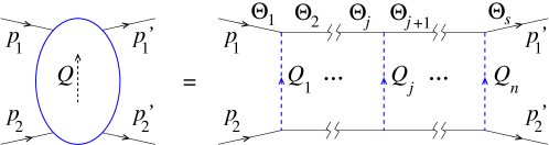
Figure 1: The scattering amplitude of two transplanckian particles (solid lines) in the eikonal approximation. Dashed lines represent (reggeized) graviton exchanges. The fast particles propagate on-shell throughout the whole eikonal chain. The angles ${\boldsymbol{\Theta}}_{j}\simeq\sum_{i=1}^{j-1}{\boldsymbol{\theta}}_{i}$ denote the direction of particle 1 w.r.t. the $z$-axis along the scattering process.

In other words, every single hit is effectively described by the elastic amplitude

$$M_{{\mathrm{el}}}({\boldsymbol{Q}}_{j})=\frac{\kappa^{2}s^{2}}{{\boldsymbol{Q}}_{j}^{2}}=\frac{\kappa^{2}s^{2}}{E^{2}{\boldsymbol{\theta}}_{j}^{2}},\quad\left(\kappa^{2}=\frac{8\pi G}{\hbar}\right)\;,$$ (2.6)

which is in turn directly connected to the phase shift $\delta_{0}$:

$$\delta_{0}(|{\boldsymbol{b}}|,E)=\frac{1}{4s}\int\frac{\mathrm{d}^{2}{\boldsymbol{Q}}}{(2\pi)^{2}}\mathrm{e}^{\frac{{\mathrm{i}{\boldsymbol{Q}}\cdot{\boldsymbol{b}}}}{\hbar}}M_{{\mathrm{el}}}({\boldsymbol{Q}})=\alpha_{G}\int\frac{\mathrm{d}^{2}{\boldsymbol{\theta}}_{s}}{2\pi{\boldsymbol{\theta}}_{s}^{2}}\mathrm{e}^{\frac{{\mathrm{i}E{\boldsymbol{\theta}}_{s}\cdot{\boldsymbol{b}}}}{\hbar}}\;.$$ (2.7)

The relatively soft nature of transplanckian scattering just mentioned is also — according to [10] — the basis for its validity in the string-gravity framework. Furthermore, the multiple-hit procedure can be generalized to multi-loop contributions in which the amplitude, for each power of $G$, is enhanced by additional powers of $s$, due to the dominance of $s$-channel iteration in high-energy spin-2 exchange versus the $t$-channel one (which provides at most additional powers of $\log s$). That is the mechanism by which the $S$-matrix exponentiates an eikonal function (or operator) with the effective coupling $\alpha_{G}\equiv Gs/\hbar$ and subleading contributions which are a power series in $R^{2}/b^{2}$.

Both the scattering angle (2.5) (and the $S$-matrix (2.2)) can be interpreted from the metric point of view [6] as the geodesic shift (and the quantum matching condition) of a fast particle in the Aichelburg-Sexl (AS) metric [41] of the other.

More directly, the associated metric emerges from the calculation [42] of the longitudinal fields coupled to the incoming particles in the eikonal series, which turn out to be

$$\frac{1}{4}h^{++}=h_{--} =2\pi Ra_{0}({\boldsymbol{x}})\delta\left(x^{-}-\pi R\epsilon(x^{+})a_{0}(b)\right)\;,$$

$$a_{0}({\boldsymbol{x}}) =\frac{1}{2\pi}\log\frac{L^{2}}{{\boldsymbol{x}}^{2}}\;,\qquad\delta_{0}(b,E)=\pi\alpha_{G}a_{0}(b)\;.$$ (2.8)

Such shock-wave expressions yield two AS metrics for the fast particles, as well as the corresponding time delay and trajectory shifts at leading level. When $b$ decreases towards $R\gg l_{s}$, corrections to the eikonal and to the effective metric involving the $R^{2}/b^{2}$ parameter have to be included, as well as graviton radiation, to which we now turn.

3 The unified single-graviton emission amplitude

We start, in the ACV framework, from the irreducible (possibly resummed [22]) eikonal, which in $D=4$ takes the form

$$\delta({\boldsymbol{b}},E)\equiv{\alpha_{G}}\left[\log\frac{L}{R}+\Delta({\boldsymbol{b}}/R)\right]=\frac{ER}{\hbar}\left[\log\frac{L}{R}+\Delta({\boldsymbol{b}}/R)\right]\;,$$ (3.1)

that we split into an IR divergent “Coulomb” contribution regularized by the cutoff $L$, and a finite part $\Delta$ which embodies the ${\boldsymbol{b}}$ dependence. The IR divergent Coulomb phase factorizes in front of the $S$-matrix [21] and should cancel out in measurable quantities. The Fourier transform of $\Delta({\boldsymbol{b}})$ defines a “potential” $\tilde{\Delta}({\boldsymbol{Q}})$ in transverse space. In particular, the leading eikonal $\delta_{0}({\boldsymbol{b}},E)={\alpha_{G}}\log(L/|{\boldsymbol{b}}|)$ corresponds to $\tilde{\Delta}({\boldsymbol{Q}})=1/{\boldsymbol{Q}}^{2}\times\Theta({\boldsymbol{Q}}^{2}-(\hbar/L)^{2})$.

Consider now, at tree level, the emission of a graviton with energy $\hbar\omega$ and transverse momentum ${\boldsymbol{q}}=\hbar\omega{\boldsymbol{\theta}}$, $|{\boldsymbol{\theta}}|$ being related to the polar emission angle while $\phi_{{\boldsymbol{\theta}}}$ is the azimuth in the transverse plane (fig. 2). Keeping in mind that the condition $\hbar\omega\ll E$ is always assumed in this paper, we can still distinguish a “Weinberg limit” in which $|{\boldsymbol{q}}|<|{\boldsymbol{Q}}|$ for which the emission amplitude is given by Weinberg’ external-line insertion formula, and a “Regge-Lipatov regime” in which $|{\boldsymbol{q}}|>|{\boldsymbol{Q}}|$ so that emission from the exchanged (and now effectively on shell) graviton has to be added. Fortunately a single, simple expression [21, 22] is able to cope simultaneously with both regimes. Let us briefly discuss how.

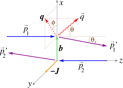
Figure 2: Center-of-mass view of the collision at impact parameter ${\boldsymbol{b}}$ of particles 1 and 2 with associated emission of a graviton $q$. The polar angles $\Theta_{s}$ and $\theta$ are related to the 2D vectors ${\boldsymbol{\Theta}}_{s}$ and ${\boldsymbol{\theta}}$ as described in eq. (2.1) and footnote 6.

Weinberg’s external insertion recipe factorizes in ${\boldsymbol{Q}}$-space (fig. 3a). This can be translated in ${\boldsymbol{b}}$-space as follows [21] (setting momentarily $\hbar=1$):

$${\cal M}^{\mathrm{soft}}_{\lambda}({\boldsymbol{b}},E,{\boldsymbol{q}},\omega)=\sqrt{{\alpha_{G}}}\frac{R}{\pi}\int\frac{\mathrm{d}^{2}{\boldsymbol{Q}}}{2\pi}\;\tilde{\Delta}({\boldsymbol{Q}})\mathrm{e}^{\mathrm{i}{\boldsymbol{Q}}\cdot{\boldsymbol{b}}}\left[\frac{E}{\omega}\,\frac{1}{2}\left(\mathrm{e}^{-\mathrm{i}\lambda(\phi_{{\boldsymbol{q}}-\frac{\omega}{E}{\boldsymbol{Q}}}-\phi_{\boldsymbol{q}})}-1\right)\right]\;,$$ (3.2)

where $\lambda=\pm 2$ is the helicity of the emitted graviton, and the factor in square brackets comes from the explicit computation of the Weinberg current on helicity states. The latter are conveniently defined by the polarization tensors [20, 21]

$$\epsilon_{\pm}^{\mu} =\frac{1}{\sqrt{2}}\left(\epsilon_{TT}^{\mu\nu}\pm\mathrm{i}\epsilon_{LT}^{\mu\nu}\right)=\frac{1}{2}\left(\epsilon_{T}^{\mu}\pm\mathrm{i}\epsilon_{L}^{\mu}\right){}\left(\epsilon_{T}^{\nu}\pm\mathrm{i}\epsilon_{L}^{\nu}\right)$$

$$\epsilon_{TT}^{\mu\nu} =\frac{1}{\sqrt{2}}\left(\epsilon_{T}^{\mu}\epsilon_{T}^{\nu}-\epsilon_{L}^{\mu}\epsilon_{L}^{\nu}\right)\;,\quad\epsilon_{LT}^{\mu\nu}=\frac{1}{\sqrt{2}}\left(\epsilon_{L}^{\mu}\epsilon_{T}^{\nu}+\epsilon_{T}^{\mu}\epsilon_{L}^{\nu}\right)$$

$$\epsilon_{T}^{\mu} =\Big{(}0,-\epsilon_{ij}\frac{q_{j}}{|{\boldsymbol{q}}|},0\Big{)}\;,\qquad\epsilon_{L}^{\mu}=\Big{(}\frac{q^{3}}{|{\boldsymbol{q}}|},\boldsymbol{0},\frac{q^{0}}{|{\boldsymbol{q}}|}\Big{)}\mp\frac{q^{\mu}}{|{\boldsymbol{q}}|}\;,$$ (3.3)

where $\epsilon_{12}=1$ and the $-$ ($+$) sign in $\epsilon_{L}^{\mu}$ corresponds to graviton emission in the forward (backward) hemisphere in the small-angle kinematics.

We note that the phase difference in (3.2) can also be written in terms of deflection angles as $\phi_{{\boldsymbol{q}}-\frac{\omega}{E}{\boldsymbol{Q}}}-\phi_{\boldsymbol{q}}=\phi_{{\boldsymbol{\theta}}-{\boldsymbol{\Theta}}_{s}}-\phi_{\boldsymbol{\theta}}$ and can be expressed by the integral representation

$$\mathrm{e}^{2\mathrm{i}\phi_{{\boldsymbol{\theta}}}}-\mathrm{e}^{2\mathrm{i}\phi_{{\boldsymbol{\theta}}^{\prime}}}=-2\int\frac{\mathrm{d}^{2}{\boldsymbol{x}}}{{2\pi x^{*}}^{2}}\left(\mathrm{e}^{\mathrm{i}\omega{\boldsymbol{x}}\cdot{\boldsymbol{\theta}}}-\mathrm{e}^{\mathrm{i}\omega{\boldsymbol{x}}\cdot{\boldsymbol{\theta}}^{\prime}}\right)\;,$$ (3.4)

where $x\equiv x_{1}+\mathrm{i}x_{2}$, $x^{*}\equiv x_{1}-\mathrm{i}x_{2}$ is the complex notation for the transverse vector ${\boldsymbol{x}}$ to be interpreted as the transverse distance between the forward outgoing hard particle and the emitted graviton. In addition, the Fourier transform (3.2) identifies ${\boldsymbol{b}}$ as the transverse distance between the two outgoing hard particles, so that ${\boldsymbol{b}}-{\boldsymbol{x}}$ is the transverse coordinate of the emitted graviton w.r.t. the backward hard particle (whose transverse position is essentially unaffected by the forward emission process), as shown in fig. 3b. In terms of such final-state variables, the impact parameter of the two incoming hard particles amounts to ${\boldsymbol{b}}_{\mathrm{in}}={\boldsymbol{b}}-\frac{\omega}{E}{\boldsymbol{x}}$. It is also interesting to note that the classical orbital angular momentum $(L^{13},L^{23})\simeq\sum_{p}E_{p}{\boldsymbol{r}}_{p}$ is conserved in the process.

Inserting eq. (3.4) into eq. (3.2), it is straightforward to perform the ${\boldsymbol{Q}}$ integrals in terms of eikonal functions of linear combinations of ${\boldsymbol{b}}$ and ${\boldsymbol{x}}$, thus yielding

$${\cal M}^{\mathrm{soft}}_{\lambda}({\boldsymbol{b}},E,{\boldsymbol{q}},\omega)=-\sqrt{{\alpha_{G}}}\frac{R}{\pi}\mathrm{e}^{\mathrm{i}\lambda\phi_{\boldsymbol{q}}}\int\frac{\mathrm{d}^{2}{\boldsymbol{x}}}{2\pi|{\boldsymbol{x}}|^{2}\mathrm{e}^{\mathrm{i}\lambda\phi_{\boldsymbol{x}}}}\;\mathrm{e}^{\mathrm{i}{\boldsymbol{q}}\cdot{\boldsymbol{x}}}\frac{E}{\omega}\Big{(}\Delta\big{(}{\boldsymbol{b}}-\textstyle{\frac{\omega}{E}}{\boldsymbol{x}}\big{)}-\Delta({\boldsymbol{b}})\Big{)}\;,$$ (3.5)

which expresses the Weinberg insertions in ${\boldsymbol{b}}$-space in terms of the eikonal functions with shifted impact parameter value ${\boldsymbol{b}}-\frac{\omega}{E}{\boldsymbol{x}}$ (fig. 3).

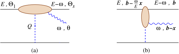
Figure 3: Single-exchange emission diagram in ${\boldsymbol{Q}}$-space with deflection angles (a), and its transverse-space counterpart with final-state variables ${\boldsymbol{b}}$, ${\boldsymbol{x}}$ and the shifted impact parameter ${\boldsymbol{b}}-\frac{\omega}{E}{\boldsymbol{x}}$ (b).

Furthermore, it was shown in [21] that the difference between the Regge and soft amplitude in the overlapping soft-central region of phase space is formally equal to (minus) the soft amplitude itself, provided one replaces the scale parameter $E$ with $\omega$. In other words, the unifying amplitude ${\cal M}^{[1]}$ matching ${\cal M}^{\mathrm{soft}}$ and ${\cal M}^{\mathrm{Regge}}$ in the corresponding phase-space validity regions can be represented as

$${\cal M}^{[1]}({\boldsymbol{b}},E,{\boldsymbol{q}},\omega)\simeq{\cal M}^{\mathrm{soft}}({\boldsymbol{b}},E,{\boldsymbol{q}},\omega)-{\cal M}^{\mathrm{soft}}({\boldsymbol{b}};\omega,{\boldsymbol{q}},\omega)\;.$$ (3.6)

In conclusion, the unified single-exchange amplitude reads

$${\cal M}^{[1]}_{\lambda}({\boldsymbol{b}},E,{\boldsymbol{q}},\omega) =-\sqrt{{\alpha_{G}}}\frac{R}{\pi}\mathrm{e}^{\mathrm{i}\lambda\phi_{\boldsymbol{q}}}\int\frac{\mathrm{d}^{2}{\boldsymbol{x}}}{2\pi|{\boldsymbol{x}}|^{2}\mathrm{e}^{\mathrm{i}\lambda\phi_{\boldsymbol{x}}}}\;\mathrm{e}^{\mathrm{i}{\boldsymbol{q}}\cdot{\boldsymbol{x}}}$$

$$\quad\times\left[\frac{E}{\omega}\Big{(}\Delta\big{(}{\boldsymbol{b}}-\textstyle{\frac{\omega}{E}}{\boldsymbol{x}}\big{)}-\Delta({\boldsymbol{b}})\Big{)}-\Big{(}\Delta({\boldsymbol{b}}-{\boldsymbol{x}})-\Delta({\boldsymbol{b}})\Big{)}\right]$$ (3.7)

$$\simeq\sqrt{{\alpha_{G}}}\frac{R}{\pi}\mathrm{e}^{\mathrm{i}\lambda\phi_{\boldsymbol{q}}}\int\frac{\mathrm{d}^{2}{\boldsymbol{x}}}{2\pi|{\boldsymbol{x}}|^{2}\mathrm{e}^{\mathrm{i}\lambda\phi_{\boldsymbol{x}}}}\;\mathrm{e}^{\mathrm{i}{\boldsymbol{q}}\cdot{\boldsymbol{x}}}\left[\Delta^{\prime}(b)\,{\boldsymbol{x}}\cdot\hat{\boldsymbol{b}}+\Delta({\boldsymbol{b}}-{\boldsymbol{x}})-\Delta({\boldsymbol{b}})\right]\;,$$ (3.8)

where, by considering an angular range $\theta=\mathcal{O}\left(1/\omega|{\boldsymbol{x}}|\right)\gg 1/Eb$ we have directly taken the $\omega=0$ limit of the “insertion function”

$$\Phi_{\mathrm{c}}\Big{(}\frac{x}{b}\Big{)}\equiv\Phi({\boldsymbol{b}},{\boldsymbol{x}},\omega=0){}=-\Delta^{\prime}(b)\,{\boldsymbol{x}}\cdot\hat{\boldsymbol{b}}+\Delta({\boldsymbol{b}})-\Delta({\boldsymbol{b}}-{\boldsymbol{x}})=\mathrm{Re}\left(\frac{x}{b}+\log\big{(}1-\frac{x}{b}\big{)}\right)\;,$$ (3.9)

which thereby acquires a classical meaning.

We notice that eq. (3.7) is directly expressed in terms of the eikonal function ${\alpha_{G}}\Delta({\boldsymbol{b}})$ of eq. (3.1), where the first (second) term in square brackets is in correspondence with external (internal) insertions, representing the Weinberg current (the high-energy correction). Furthermore, the Weinberg part is proportional to the classical scattering angle $\Theta_{s}=2R\Delta^{\prime}(b)$ and produces the leading $1/\omega$ behaviour of the amplitude.

By then replacing (3.9) into (3.7) we obtain the single-exchange emission amplitude in the soft-based representation (e.g. for $\lambda=-2$)

$${\cal M}^{[1]}({\boldsymbol{b}},E;{\boldsymbol{q}},\omega)=\sqrt{{\alpha_{G}}}\frac{R}{2}\frac{q^{*}}{q}\int\mathrm{d}^{2}{\boldsymbol{x}}\;\mathrm{e}^{\mathrm{i}{\boldsymbol{q}}\cdot{\boldsymbol{x}}}h_{s}({\boldsymbol{b}},{\boldsymbol{x}})\;,$$ (3.10)

where the soft field $h_{s}$ — in the small-deflection regime described by the leading eikonal — has the expression

$$h_{s}({\boldsymbol{b}},{\boldsymbol{x}})=-\frac{\mathrm{Re}\left(\frac{x}{b}+\log\big{(}1-\frac{x}{b}\big{)}\right)}{\pi^{2}x^{*2}}\;.$$ (3.11)

4 Infrared logs in the elastic eikonal phase

The long distance features of the Coulomb-like interaction mentioned before at leading level $\sim{\alpha_{G}}$, affect gravitational scattering at higher orders as well. ACV [14] provided a calculation of the next few orders in the eikonal, which in our massless transplanckian scattering involve the parameters $l_{p}^{2}/b^{2}$ and $R^{2}/b^{2}$ introduced before. Here we recall those results, and we illustrate them in order to gain some better understanding of the role of the IR singularity for graviton radiation as well.

Due to the exponentiation of the $S$-matrix in impact parameter space, we have the second-order expansion

$$S_{\mathrm{el}}=\mathrm{e}^{2\mathrm{i}\delta(b,E)}=\mathrm{e}^{2\mathrm{i}(\delta_{0}+\delta_{1}+\delta_{2}+\cdots)}=1+2\mathrm{i}(a^{(0)}+a^{(1)}+a^{(2)}+\cdots)$$ (4.1)

where fixed-order amplitudes $a^{(n)}$ are related to the eikonal coefficients $\delta^{(n)}$ as follows:

$$a^{(0)} =\delta_{0}=\frac{Gs}{\hbar}\log\frac{L}{b}=\frac{Gs}{\hbar}\left(\log\frac{L}{R}+\log\frac{R}{b}\right)$$ (4.2)

$$a^{(1)} =\mathrm{i}\delta_{0}^{2}+\delta_{1}\;,$$ (4.3)

$$a^{(2)} =-\frac{2}{3}\delta_{0}^{3}+2\mathrm{i}\delta_{0}\delta_{1}+\delta_{2}\;.$$ (4.4)

We noticed already that the cutoff dependence in $a_{0}$ is additive in impact parameter space, and is thus factorizable in the $S$-matrix as a pure overall phase, which is, by itself, unobservable. But we want to look at higher orders also, and in particular at order ${\alpha_{G}}R^{2}/b^{2}$. For such terms the ACV method was to compute the imaginary parts of the measurable parameters $\delta_{1},\,\delta_{2}$ as required by unitarity diagrams, and to derive the real parts by analyticity and asymptotic behaviour arguments. For pure gravity they set

$$\mathrm{Im\,}\delta_{1} =0=\mathrm{Im\,}a^{(1)}-\delta_{0}^{2}$$ (4.5)

$$\mathrm{Im\,}\delta_{2} =\mathrm{Im\,}a^{(H)}\;,\qquad\text{yielding in total}$$ (4.6)

$$\mathrm{Im\,}a^{(2)} =2\delta_{0}\delta_{1}+\mathrm{Im\,}a^{(H)}$$ (4.7)

In eq. (4.7) the first term represents the 2-body discontinuity and the second one the $2\to 3$ contribution to $\mathrm{Im\,}\delta_{2}$, due to graviton radiation in the central region, as embodied in the H-diagram (fig. 4). At this point, ACV looked for analytic functions of the Mandelstam variables having the correct discontinuities and asymptotic behaviours of $\delta_{1}$ and $\delta_{2}$, so as to determine both.

Figure 4: The H diagram providing the first subleading correction to the eikonal phase.

At one-loop level, starting from eq. (4.5), they found only one analytic structure, yielding

$$a^{(1)}=\mathrm{i}\delta_{0}^{2}+\delta_{1}=\left(\mathrm{i}+\frac{3}{\pi}\log s\frac{\hbar^{2}\nabla_{\boldsymbol{b}}^{2}}{s}\right)\delta_{0}^{2}(b,E)$$ (4.8)

and thus determining in this way the one-loop coefficient

$$\delta_{1}=\frac{6}{\pi}\frac{Gs}{\hbar}\frac{l_{p}^{2}}{b^{2}}\log s=\frac{6}{\pi}\frac{G^{2}s}{b^{2}}\log s\qquad\text{(pure gravity)}\;.$$ (4.9)

The above result for $\delta_{1}$ is consistent with what has been obtained starting from supergravity calculations [43] after subtracting [44] the gravitino contribution. We also checked that it agrees with more recent estimates [45]. We are not aware, instead, of any independent calculation of $\delta_{2}$.

At two-loop level the situation is more involved because the H-diagram predicts [14] the $D=4$ absorptive part

$$\mathrm{Im\,}\delta_{2}=\mathrm{Im\,}a^{(H)} =\log s\;\frac{Gs}{\hbar}(\pi R)^{2}\int\mathrm{d}^{2}x\;|h(b,x)|^{2}$$

$$=\frac{R^{2}}{\pi b^{2}}\left(\delta_{0}+\text{finite part}\right)\log s\;,$$ (4.10)

$$h(b,x) \equiv\frac{x-x^{*}}{2\pi^{2}bx^{*}(x-b)}\;,$$ (4.11)

where the field $h$ was introduced in [16] and, in parallel with $h_{s}$, is related to the metric coefficient $h_{zz^{*}}$ ($h_{z^{*}z^{*}}$ for $h_{s}$) of the ACV metric [21]. Since $|h(x)|=\mathcal{O}\left(1/|x|\right)$, the result (4.10) carries the logarithmic IR divergence parametrized by $\delta_{0}$. Furthermore, $2\delta_{0}\delta_{1}$ turns out to be of the same order as $\mathrm{Im\,}a^{H}$ by building up a total $\mathrm{Im\,}a^{(2)}$ in eq. (4.7) which is 4 times larger than $\mathrm{Im\,}a^{(H)}$.

That divergence is actually to be expected in the imaginary part, in order to compensate a similar divergence of virtual corrections, so as to yield a finite total emission probability. The trouble would be if the divergence of $\mathrm{Im\,}a^{(H)}=\mathrm{Im\,}\delta_{2}$ were transferred to $\mathrm{Re}\delta_{2}$, because it would mean an IR singularity of a measurable quantity which is incurable, due to its multiplicative $b$-dependence.

Fortunately ACV were able to show that the IR divergence cancels out in $\mathrm{Re}\delta_{2}$, which is finite, thus leading to a no-renormalization argument for the infinite Coulomb phase at order $G^{3}s^{2}$. In fact, by the same analyticity and asymptotic behaviour arguments used before, they found a unique solution to eqs. (4.7) and (4.10) for $a^{(2)}$, given by the superposition of two analytic structures

$$a^{(2)}=\left(1+2\frac{\hbar^{2}\nabla_{{\boldsymbol{b}}}^{2}}{s}\right)\left(-\frac{2}{3}\delta_{0}^{3}\right)+2\left(1+\frac{2\mathrm{i}}{\pi}\log s\right)\left(\frac{\hbar^{2}\nabla_{{\boldsymbol{b}}}^{2}}{s}\Big{(}\frac{2}{3}\delta_{0}^{3}\Big{)}+\frac{G^{3}s^{2}}{\hbar b^{2}}\right)\;.$$ (4.12)

Here the first term contains the leading iteration of the 2-body eikonal and definite subleading contributions, while the second term contains also the finite part of the H-diagram contribution, computed in [14] in dimensional regularization.  By working out the $\nabla^{2}$ terms, we can check that the IR singular $\mathrm{Im\,}a^{(2)}$ is consistent with eq. (4.7), while the divergence of the real part cancels out between the two terms. In conclusion, we do not need any new divergent Coulomb phase at order $G^{3}s^{2}$. The outcome of the calculation is just the finite result

$$\mathrm{Re}\delta_{2}=\frac{Gs}{\hbar}\frac{R^{2}}{2b^{2}}\;,$$ (4.13)

which provides the first correction to both the eikonal and the Einstein deflection angle at relative order $R^{2}/b^{2}$. In the Breit frame for scattering ACV found the deflection

$$\sin\frac{1}{2}\Theta_{s}(b)=\frac{R}{b}\left(1+\frac{R^{2}}{b^{2}}\right)\;.$$ (4.14)

5 Infrared logs in radiation and eikonal resummation

So far, following [21, 18] we have constructed a graviton radiation amplitude unifying the fragmentation and central emission regions in our eikonal approach. We have shown that the effect of the large-distance gravitational interaction cancels out at the level of the (infinite) scattering phase. Here we investigate the same question at the level of gravitational radiation.

Indeed, we meet immediately a possible problem at the single-graviton exchange level. The amplitude (say, for helicity $\lambda=-2$) is directly related to the field $h_{s}$ of eq. (3.11) by a Fourier transform:

$${\cal M}^{(1)}_{\lambda=-2}({\boldsymbol{b}},{\boldsymbol{q}})=\sqrt{{\alpha_{G}}}\frac{R}{2}\frac{q^{*}}{q}\int\mathrm{d}^{2}{\boldsymbol{x}}\;\mathrm{e}^{\mathrm{i}{\boldsymbol{q}}\cdot{\boldsymbol{x}}/\hbar}h_{s}(b,x)\;.$$ (5.1)

Here the integral is linearly IR divergent by power counting, due to the large-${\boldsymbol{x}}$ behaviour $\sim 1/|{\boldsymbol{x}}|$ of $h_{s}$ (and $h$). Nevertheless, the Fourier Transform can be done thanks to the oscillating factor $\mathrm{e}^{\mathrm{i}{\boldsymbol{x}}\cdot\omega{\boldsymbol{\theta}}}$ and yields the expression

$${\cal M}^{(1)} =\mathrm{e}^{\frac{\mathrm{i}}{2}{\boldsymbol{q}}\cdot{\boldsymbol{b}}}\sqrt{{\alpha_{G}}}\frac{R}{\pi}\;\mathrm{Re}\left[\mathrm{e}^{-\frac{\mathrm{i}}{2}{\boldsymbol{q}}\cdot{\boldsymbol{b}}}\frac{\mathrm{i}}{\pi}\left(\frac{1}{q^{*}b}-\int_{0}^{\infty}\frac{\mathrm{d}t\;\mathrm{e}^{-t}}{q^{*}b-2\mathrm{i}t}\right)\right]$$

$$\stackrel{{\scriptstyle bq\to 0}}{{\simeq}}\sqrt{{\alpha_{G}}}\frac{R}{\pi}\left[-\frac{\sin\phi_{\boldsymbol{q}}}{|qb|}+\frac{1}{2}\log\frac{2}{|qb|}+\text{const in }qb\right]\qquad(|\theta|\gg\theta_{m})$$ (5.2)

We note that the expected soft behaviour $\sim 1/\omega$ is accompanied by a logarithmic one, probably related to the proposal in [27] and that both involve the variable $b{\boldsymbol{q}}$ by showing a strong ${\boldsymbol{\theta}}$-dependence, which is not square-integrable at ${\boldsymbol{q}}=\omega{\boldsymbol{\theta}}\to 0$, and — as it stands — is not usable for physical spectra.

In other words, here we stress the point that the single-exchange amplitude is very sensitive to the IR in the span $0<|{\boldsymbol{x}}|<\hbar/|{\boldsymbol{q}}|$ and shows a spurious singularity at ${\boldsymbol{q}}=0$ due to large distances, despite the absence of collinear singularities in the matrix element. But the way out this potential problem is just the correct use of the single-exchange amplitude as an intermediate result, in order to calculate the complete one. In fact, we know from start that we have to sum over all possible exchanges in order to be able to reach physical deflection angles of order $\Theta_{E}=2R/b\gg\theta_{m}=\hbar/(bE)$. Such resummation is possible because of high-energy factorization [21] at fixed impact parameter ${\boldsymbol{b}}$, and takes into account the fact that the incidence angles of the various contributions are rotated, so as to cover, eventually, the larger angular range $\theta_{m}\ll|{\boldsymbol{\theta}}|\sim 2R/b<1$ they are required to describe. By working out that procedure it was found [21] that the two contributions in eq. (3.8) exponentiate independently by yielding the result

$${\cal M}_{\lambda} =\mathrm{e}^{2\mathrm{i}\delta(b,E)}\;\mathfrak{M}_{\lambda}({\boldsymbol{b}},E,{\boldsymbol{q}},\omega)$$

$$2\mathrm{i}\omega\mathfrak{M}_{\lambda} =\frac{\sqrt{{\alpha_{G}}}}{\pi}\mathrm{e}^{\mathrm{i}\lambda\phi_{\boldsymbol{\theta}}}\int\frac{\mathrm{d}^{2}\zeta}{2\pi|\zeta|^{2}}\mathrm{e}^{-\mathrm{i}\lambda\phi_{\zeta}}\;\mathrm{e}^{\mathrm{i}{\boldsymbol{\zeta}}\cdot{\boldsymbol{\theta}}}\left(\mathrm{e}^{-2\mathrm{i}\omega R\log\left|\hat{b}-\frac{{\boldsymbol{\zeta}}}{\omega b}\right|}-\mathrm{e}^{-\mathrm{i}{\boldsymbol{\zeta}}\cdot{\boldsymbol{\Theta}}_{s}}\right)$$

$$=\frac{\sqrt{{\alpha_{G}}}}{\pi}\mathrm{e}^{\mathrm{i}\lambda\phi_{\boldsymbol{\theta}}}\int\frac{\mathrm{d}^{2}\zeta}{2\pi|\zeta|^{2}}\mathrm{e}^{-\mathrm{i}\lambda\phi_{\zeta}}\;\mathrm{e}^{\mathrm{i}{\boldsymbol{\zeta}}\cdot({\boldsymbol{\theta}}-{\boldsymbol{\Theta}}_{s})}\left(\mathrm{e}^{-2\mathrm{i}\omega R\Phi_{\mathrm{c}}\big{(}\frac{{\boldsymbol{\zeta}}}{b\omega}\big{)}}-1\right)\;,$$ (5.3)

in terms of the rescaled variable ${\boldsymbol{\zeta}}\equiv b\omega{\boldsymbol{z}}=\omega{\boldsymbol{x}}$. This is in complete agreement with the result of the fully classical calculation of [18].

We note that, because of (5.3), resummation involves the phase factor $\mathrm{e}^{-2\mathrm{i}\omega R\Phi_{\mathrm{c}}}$ to keep coherence on the ${\boldsymbol{x}}$-space involved. In practice that means that we should require, qualitatively, that $1\leq|\Phi_{\mathrm{c}}({\boldsymbol{x}}/b)|\leq 1/(2\omega R)$ for coherence to be reached, thus reducing the IR sensitivity span to $b<|{\boldsymbol{x}}|<1/(\omega\Theta_{E})$. In other words, the $|{\boldsymbol{\theta}}|$-dependence is regularized around $\Theta_{E}=2R/b$, way before reaching the IR singularity peak. As a consequence, our resummed amplitudes are finite in the small-$\omega$ region and well-behaved on the whole physical phase space.

Finally, we resum the independent emissions of many gravitons whose amplitudes are factorized in terms of the emission factor $\mathfrak{M}$ of eq. (5.3). The $S$-matrix operator acting on the Fock space of gravitons is then obtained by including virtual corrections which are incorporated by exponentiating both creation ($a^{\dagger}_{\lambda}(\vec{q})$) and destruction ($a_{\lambda}(\vec{q})$) operators of definite helicity $\lambda$ as follows

$$\hat{S}=\mathrm{e}^{2\mathrm{i}\delta({\boldsymbol{b}},E)}\exp\left\{\int\frac{\mathrm{d}^{3}q}{\sqrt{2\omega}}\;2\mathrm{i}\left[\sum_{\lambda}\mathfrak{M}_{\lambda}({\boldsymbol{b}},\vec{q})a^{\dagger}_{\lambda}(\vec{q})+\text{h.c.}\right]\right\}\;.$$ (5.4)

Such a simple coherent state assumes negligible correlations among the emitted gravitons, an assumption which is certainly justified by the factorization theorems [29] of multiple soft graviton emission. We believe this to be still a good approximation in the region $\omega R<1$ discussed in this work. Such an $S$-matrix is unitary because of the hermitian operator appearing in the exponent. It also conserves energy as long as we limit ourselves to processes in which the total energy carried by the emitted gravitons is much smaller than $\sqrt{s}$.

Given (5.4) it is straightforward to compute the energy carried by the gravitons as a function of $\omega$, ${\boldsymbol{\theta}}$ and $\lambda$, in terms of the expectation value of the corresponding operator $\hbar\omega a^{\dagger}_{\lambda}(\vec{q})a_{\lambda}(\vec{q})$. Using standard properties of coherent states this is just given by

$$\frac{\mathrm{d}E^{\mathrm{GW}}}{\mathrm{d}\omega\,d^{2}{\boldsymbol{\theta}}}=2\hbar\sum_{\lambda=\pm 2}|\omega\mathfrak{M}_{\lambda}({\boldsymbol{b}},\vec{q})|^{2}\;,$$ (5.5)

which is directly related to the spectrum in the small-angle kinematics (2.1) and has a smooth classical limit since ${\alpha_{G}}$ is $\mathcal{O}\left(\hbar^{-1}\right)$. The explicit calculation will be carried out in sec. 6.

6 Small-$\boldsymbol{\omega}$ behaviour of the radiation amplitude

In this section we will study the gravitational radiation spectrum $\frac{\mathrm{d}E^{\mathrm{GW}}}{\mathrm{d}\omega}$ in the small-$\omega$ region, here defined by $\omega R<(\ll)1$. Since, throughout this paper, we work at leading order in the scattering angle $\Theta_{s}=2R/b\ll 1$, this region is actually divided in two subregions: $\omega b<(\ll)1$ and $\omega b>(\gg)1$. In the complementary regions $\omega R=\mathcal{O}\left(1\right)$ and $\omega R>(\gg)1$, analyzed in detail in [18, 20, 21], decoherence effects — related to the exponentiation of $2\omega R\Phi_{\mathrm{c}}$ in eq. (5.3) — suppress the integration region $\theta>\Theta_{s}$ and creates a break in the spectrum around “Hawking’s frequency” $\omega\sim R^{-1}$, with a $1/(\omega R)$ tail. The whole treatment then becomes unreliable above $\omega R\sim\Theta_{s}^{-2}$. We will have nothing more to say here about the $\omega R>1$ regime.

On the other hand, in the small-$\omega R$ region, there is a clear distinction between the two above-mentioned (sub)regimes $\omega b<(\ll)1$ and $\omega b>(\gg)1$. Before turning to their quantitative study let us anticipate some qualitative aspects of each.

• For $\omega b<(\ll)1$ we find corrections to the ZFL in the form of an expansion in powers of $\omega R$ which get enhanced by logarithms of $\omega b$. Even if small, these corrections (not considered in the earlier treatments of [18, 20, 21]) are obviously important for determining whether the spectrum is (or is not) maximal at the ZFL. Furthermore, since the ZFL itself is of $\mathcal{O}\left(\Theta_{s}^{2}\right)$, the $\mathcal{O}\left(\omega R\log(\omega b)\right)$ and $\mathcal{O}\left(\omega^{2}R^{2}\log^{2}(\omega b)\right)$ leading corrections turn out to be of relative order $\mathcal{O}\left(\omega b\log(\omega b)\right)$ and $\mathcal{O}\left(\omega^{2}b^{2}\log^{2}(\omega b)\right)$, respectively. The first one, while representing an interesting memory effect on the wave form and a contribution to the polarized flux, does not contribute to the unpolarized and/or azimuthally-averaged flux. The second represents instead the leading contribution to the unpolarized and/or angle-integrated flux. Its positivity implies necessarily a maximum of the spectrum away from $\omega=0$. Finally, we will be able to resum all the leading logs in terms of an IR-finite Coulomb phase.

• For $\omega b>1$ the above-mentioned logarithmic enhancements disappear and, instead, a cutoff intervenes at $\theta\sim(\omega b)^{-1}$. As a result, the maximum of the spectrum is reached at $\omega b=\mathcal{O}\left(1\right)$: numerically, it is found to stay, independently of $\Theta_{s}$, around $\omega b\sim 0.5$. For $\omega b\gg 1\gg\omega R$ a previously studied regime settles in, in which the spectrum decreases like $\log(1/\omega R)$ [18, 20, 21].

After recasting eq. (5.3) in a more convenient form, we shall recover, in sec. 6.1, the leading-$\omega$ contributions in the region $0<\omega R<1$, while in sec. 6.2 we compute the new sub-leading corrections and the emergence of a peak in the spectrum at $\omega b\sim 0.5$.

We start by defining

$$A^{(\lambda)}\equiv\frac{2\pi\mathrm{i}\omega\mathfrak{M}_{\lambda}}{\sqrt{{\alpha_{G}}}}=A^{(\lambda)}_{L}+A^{(\lambda)}_{NL}$$ (6.1)

where, using eq. (5.3), we can identify:

$$A^{(\lambda)}_{L}=\int_{0}^{\infty}\frac{\mathrm{d}r}{r}\int_{0}^{2\pi}\frac{\mathrm{d}\phi_{x}}{2\pi}\;\mathrm{e}^{\mathrm{i}\lambda(\phi_{{\boldsymbol{\theta}}}-\phi_{x})}\left(\mathrm{e}^{\mathrm{i}\omega{\boldsymbol{x}}\cdot{\boldsymbol{\theta}}}-\mathrm{e}^{\mathrm{i}\omega{\boldsymbol{x}}\cdot({\boldsymbol{\theta}}-{\boldsymbol{\Theta}}_{s})}\right)$$ (6.2)

and

$$A^{(\lambda)}_{NL}=\int_{0}^{\infty}\frac{\mathrm{d}r}{r}\int_{0}^{2\pi}\frac{\mathrm{d}\phi_{x}}{2\pi}\;\mathrm{e}^{\mathrm{i}\lambda(\phi_{{\boldsymbol{\theta}}}-\phi_{x})}\mathrm{e}^{\mathrm{i}\omega{\boldsymbol{x}}\cdot{\boldsymbol{\theta}}}\left(\mathrm{e}^{-\mathrm{i}\omega R\log(\hat{{\boldsymbol{b}}}-\frac{{\boldsymbol{x}}}{b})^{2}}-1\right)\;.$$ (6.3)

In order to evaluate $A_{NL}$, we will use the expansion:

$$\log(\hat{{\boldsymbol{b}}}-\frac{{\boldsymbol{x}}}{b})^{2}=\log(1+\frac{r^{2}}{b^{2}})+\log(1-2\frac{{\boldsymbol{b}}\cdot{\boldsymbol{x}}}{b^{2}+r^{2}})=\log(1+\frac{r^{2}}{b^{2}})-2\frac{{\boldsymbol{b}}\cdot{\boldsymbol{x}}}{b^{2}+r^{2}}+\dots\,,$$ (6.4)

which is valid both at large and at small $r/b$. By replacing (6.4) into (6.3), we rewrite

$$A^{(\lambda)}_{NL}\simeq\int_{0}^{\infty}\frac{\mathrm{d}r}{r}\int_{0}^{2\pi}\frac{\mathrm{d}\phi_{x}}{2\pi}\;\mathrm{e}^{\mathrm{i}\lambda(\phi_{{\boldsymbol{\theta}}}-\phi_{x})}\left[\mathrm{e}^{\mathrm{i}\omega{\boldsymbol{x}}\cdot({\boldsymbol{\theta}}-{\boldsymbol{\Theta}_{s,r}})}\mathrm{e}^{-\mathrm{i}\omega R\log(1+\frac{r^{2}}{b^{2}})}-\mathrm{e}^{\mathrm{i}\omega{\boldsymbol{x}}\cdot{\boldsymbol{\theta}}}\right]\;,$$ (6.5)

where we have introduced what we call the rescattering deflection angle ${\boldsymbol{\Theta}_{s,r}}\equiv{\boldsymbol{\Theta}}_{s}/(1+r^{2}/b^{2})$ which, together with the eikonal phase $\omega R\log(1+r^{2}/b^{2})$, describes the rescattering evolution of the emitted graviton.

We then split the $r$-integration into two regions: $r<(\ll)b$, and $r>(\gg)b$. In the small-$r$ region, ${\boldsymbol{\Theta}_{s,r}}\simeq{\boldsymbol{\Theta}}_{s}$, the ${\boldsymbol{\Theta}}_{s}$-dependence cancels out between $A_{L}$ and $A_{NL}$ and can be eliminated in their sum. Performing now the azimuthal integrations in terms of Bessel functions, we obtain

$$A_{L}^{(\lambda)}=\int_{b}^{\infty}\frac{\mathrm{d}r}{r}\left[\mathrm{e}^{\mathrm{i}\lambda\psi}J_{2}(\omega r|{\boldsymbol{\theta}}-{\boldsymbol{\Theta}}_{s}|)-J_{2}(\omega r\theta)\right]\;,\qquad\psi\equiv(\phi_{{\boldsymbol{\theta}}}-\phi_{{\boldsymbol{\theta}}-{\boldsymbol{\Theta}}_{s}})\;,$$ (6.6)

where $\psi$ is the azimuthal-angle transfer in scattering (see fig. 5), and

$$A_{NL}^{(\lambda)}\simeq\int_{b}^{\infty}\frac{\mathrm{d}r}{r}\left[J_{2}(\omega r\theta)-\mathrm{e}^{\mathrm{i}\lambda\psi_{r}}\mathrm{e}^{-\mathrm{i}\omega R\log(1+\frac{r^{2}}{b^{2}})}J_{2}(\omega r|{\boldsymbol{\theta}}-{\boldsymbol{\Theta}_{s,r}}|)\right]\;,\qquad\psi_{r}\equiv(\phi_{{\boldsymbol{\theta}}}-\phi_{{\boldsymbol{\theta}}-{\boldsymbol{\Theta}_{s,r}}})\;,$$ (6.7)

where $\psi_{r}$ is the analogue azimuthal transfer in rescattering. Furthermore, the $r$-integration is now limited to the large-$r$ region.

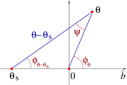
Figure 5: Picture of the polar and azimuthal angles in the transverse plane. ${\boldsymbol{\Theta}}_{s}$ and ${\boldsymbol{\theta}}$ correspond respectively to the projections of the unit-vectors $\hat{p}_{1}{}^{\prime}$ and $\hat{q}$ on the $\langle x,y\rangle$-plane of fig. 2. In this configuration, all azimuthal angles $\phi_{j}$ and $\psi$ are positive.

Since ${\boldsymbol{\Theta}_{s,r}}\ll 1$ in the large-$r$ region, we neglect it in the argument of the Bessel function in eq. (6.7), to get the simplified form

$$A_{NL}^{(\lambda)} \simeq\int_{b}^{\infty}\frac{\mathrm{d}r}{r}\;J_{2}(\omega r\theta)\left[\left(1-\mathrm{e}^{-\mathrm{i}\omega R\log(1+\frac{r^{2}}{b^{2}})}\right)+\mathrm{e}^{-\mathrm{i}\omega R\log(1+\frac{r^{2}}{b^{2}})}(1-\mathrm{e}^{\mathrm{i}\lambda\psi_{r}})\right]$$

$$\equiv A_{NL,C}+\delta A_{NL}^{(\lambda)}\;,$$ (6.8)

where the eikonal-phase contribution $A_{NL,C}$ is the main one to be discussed below, while the rescattering phase can be further expanded to first order in ${\boldsymbol{\Theta}_{s,r}}$:

$$1-\mathrm{e}^{\mathrm{i}\lambda\psi_{r}}\simeq-\mathrm{i}\lambda\psi_{r}=-\mathrm{i}\lambda\frac{\Theta_{s}\sin\phi_{\boldsymbol{\theta}}}{\theta(1+\frac{r^{2}}{b^{2}})}$$ (6.9)

and is correspondingly small. By replacing that value into (6.8) we obtain

$$\delta A_{NL}^{(\lambda)} \simeq-\mathrm{i}\lambda\frac{\Theta_{s}\sin\phi_{\boldsymbol{\theta}}}{\theta}\int_{b}^{\infty}\frac{\mathrm{d}r}{r}\;\frac{J_{2}(\omega r\theta)}{1+\frac{r^{2}}{b^{2}}}\mathrm{e}^{-\mathrm{i}\omega R\log(1+\frac{r^{2}}{b^{2}})}$$

$$\stackrel{{\scriptstyle b\omega\ll 1}}{{=}}-\mathrm{i}\lambda\frac{\Theta_{s}\sin\phi_{\boldsymbol{\theta}}}{\theta}\left[\frac{(b\omega\theta)^{2}}{4}\log\frac{C}{b\omega\theta}+\omega R\text{-corrections}\right]\;,$$ (6.10)

where the latter estimate comes from the small-$x$ Bessel expansion $J_{2}(x)\simeq x^{2}/4$ and $C$ parametrizes the upper limit of that regime.

We thus see that there is a logarithmic enhancement of the nominal $(b\omega\theta)^{2}$ behaviour of $\delta A_{NL}^{(\lambda)}$, but is not the maximal one. For that reason, in the following we shall mostly focus on the term $A_{NL,C}$ of (6.8), which will be shown to contain leading-log contributions and to be related to the Coulomb phase of rescattering.

By then leaving $\delta A_{NL}^{(\lambda)}$ aside for the time being, and with the approximation $\log(1+\frac{r^{2}}{b^{2}})\simeq\log(\frac{r^{2}}{b^{2}})$ in the exponents, we can write

$$A^{(\lambda)}-\delta A_{NL}^{(\lambda)} =\int_{b}^{\infty}\frac{\mathrm{d}r}{r}\;\left[\mathrm{e}^{\mathrm{i}\lambda\psi}J_{2}(\omega r|{\boldsymbol{\theta}}-{\boldsymbol{\Theta}}_{s}|)-J_{2}(\omega r\theta)\right]$$

$$\quad+\int_{b}^{\infty}\frac{\mathrm{d}r}{r}\left(1-\mathrm{e}^{-\mathrm{i}\omega R\log(\frac{r^{2}}{b^{2}})}\right)J_{2}(\omega r\theta)$$

$$=\left[\mathrm{e}^{\mathrm{i}\lambda\psi}\frac{J_{1}(\omega b|{\boldsymbol{\theta}}-{\boldsymbol{\Theta}}_{s}|)}{\omega b|{\boldsymbol{\theta}}-{\boldsymbol{\Theta}}_{s}|}-\frac{J_{1}(\omega b\theta)}{\omega b\theta}\right]+2i\omega R\int_{\omega b\theta}^{\infty}\frac{\mathrm{d}\rho}{\rho^{2}}\;J_{1}(\rho)\left(\frac{\rho}{b\omega\theta}\right)^{-2\mathrm{i}\omega R}\;,$$ (6.11)

where we have used a well-known Bessel integral and the last term (carrying an explicit $\omega R$ factor) is obtained through an integration by parts. In the following two subsections we will stick, for simplicity, to this simpler analytic approximation which is sufficient to discuss the qualitative feature of the spectrum. However, in sec. 6.3, we will compare numerical results with the better approximation given in eqs. (6.2),(6.5).

Note that the amplitudes for $\lambda=\pm 2$ are not each other’s complex conjugates. Equation (6) is a convenient starting point for analyzing various limits. In particular, the subleading corrections enhanced at leading logarithmic level come from the last term.

6.1 The leading amplitude for $\boldsymbol{\omega R<1}$

Inspection of the small-$\omega$ behaviour of the last term in eq. (6) shows that it vanishes in the $\omega\rightarrow 0$ limit. Limiting ourselves to the first two terms we note first that the $J_{1}$ terms are leading and close to $1/2$ for small values of the argument $\mathcal{O}\left(bq\right)<1$. That is, for $1>\theta>\Theta_{s}$ eq. (6) becomes

$$A_{L}^{(\lambda)}\simeq\frac{J_{1}(\omega b\theta)}{\omega b\theta}\left(\mathrm{e}^{\mathrm{i}\lambda\psi}-1\right)$$ (6.12)

and yields

$$\frac{\mathrm{d}E_{\lambda}^{\mathrm{GW}}}{\mathrm{d}\omega\mathrm{d}\Omega}=2\hbar|\omega\mathfrak{M}_{\lambda}|^{2} \simeq\frac{Gs}{8\pi^{2}}\left|\frac{2J_{1}(bq)}{bq}\right|^{2}\left|\mathrm{e}^{\mathrm{i}\lambda\psi}-1\right|^{2}$$

$$=\frac{Gs}{2\pi^{2}}\left|\frac{2J_{1}(bq)}{bq}\right|^{2}\,\frac{\sin^{2}\phi_{\boldsymbol{\theta}}}{|{\boldsymbol{\theta}}-{\boldsymbol{\Theta}}_{s}|^{2}}\,\Theta_{s}^{2}\;.$$ (6.13)

where we have used the trigonometric relation (see fig. 5): $\sin\psi=\frac{\Theta_{s}}{|{\boldsymbol{\theta}}-{\boldsymbol{\Theta}}_{s}|}\sin\phi_{\theta}$.

On the other hand, $bq>1$ is allowed by phase space if $b\omega>1$, and in that case the $J_{1}$ factors suppress the amplitude, consistently with previous estimates [21] of the large $bq$ behaviour. By integrating over the angular phase space we then find the $\lambda$-independent result:

$$\frac{\mathrm{d}E_{\lambda}^{\mathrm{GW}}}{\mathrm{d}\omega} \simeq\frac{Gs}{\pi}\int_{0}^{1}\frac{\mathrm{d}\theta}{\theta}\;\left|\frac{2J_{1}(b\omega\theta)}{b\omega\theta}\right|^{2}\min\{\theta^{2},\Theta_{s}^{2}\}$$

$$\simeq\frac{Gs}{\pi}\int_{0}^{\min\{1,1/b\omega\}}\frac{\mathrm{d}\theta}{\theta}\;\min\{\theta^{2},\Theta_{s}^{2}\}$$

$$=\frac{Gs}{\pi}\Theta_{s}^{2}\left[\log\min\big{(}\frac{1}{\Theta_{s}},\frac{1}{2\omega R}\big{)}+\text{const}\right]\;.$$ (6.14)

Note that the spectrum takes the ZFL form for $\omega<b^{-1}$ but differs by the phase-space condition $\theta<(b\omega)^{-1}$ (or $bq<1$) for $\omega>b^{-1}$, as required by the large-log assumption. As a consequence, the full frequency spectrum has a $\log(1/\omega R)$ dependence of the form:

$$\frac{\mathrm{d}E^{\mathrm{GW}}}{\mathrm{d}\omega}=\frac{Gs}{\pi}\Theta_{s}^{2}\left[\text{const}+2\log\big{(}\frac{1}{2\omega R}\big{)}\right]\;,$$ (6.15)

which saturates at $\omega=b^{-1}$, reaching the ZFL value.

6.2 Subleading corrections and IR-sensitive logs

Enhanced subleading corrections come entirely from the last term in eq. (6). As a matter of fact that term is known exactly in terms of an hypergeometric function:

$$2\mathrm{i}\omega R\int_{\omega b|\theta|}^{\infty}\frac{\mathrm{d}\rho}{\rho^{2}}\;J_{1}(\rho)\left(\frac{\rho}{b\omega\theta}\right)^{-2\mathrm{i}\omega R}\equiv\Delta_{C}(\omega R,\omega b\theta)$$

$$=\frac{1}{2}\,_{1}F_{2}(-\mathrm{i}\omega R;2,1-\mathrm{i}\omega R;-\frac{\omega^{2}b^{2}\theta^{2}}{4})-\frac{1}{2}\frac{\Gamma(1-\mathrm{i}\omega R)}{\Gamma(1+\mathrm{i}\omega R)}\frac{(\frac{b\omega\theta}{2})^{2\mathrm{i}\omega R}}{1+\mathrm{i}\omega R}$$ (6.16)

We may now collect all terms in $A^{(\lambda)}$,

$$A^{(\lambda)}=\left[\mathrm{e}^{\mathrm{i}\lambda\psi}\frac{J_{1}(\omega b|{\boldsymbol{\theta}}-{\boldsymbol{\Theta}}_{s}|)}{\omega b|{\boldsymbol{\theta}}-{\boldsymbol{\Theta}}_{s}|}-\frac{J_{1}(\omega b\theta)}{\omega b\theta}\right]+\Delta_{C}(\omega R,\omega b\theta)$$ (6.17)

and note that the two definite-helicity amplitudes differ just by an imaginary term proportional to $\sin 2\psi$. On the other hand, if we consider the more conventional linear polarizations:

$$A^{(\times)}=A_{LT}=\frac{i}{\sqrt{2}}(A^{(2)}-A^{(-2)})\;;\qquad A^{(+)}=A_{TT}=\frac{1}{\sqrt{2}}(A^{(2)}+A^{(-2)})$$ (6.18)

we see that the $\lambda$-dependent term in eq. (6.17) only contributes to $A^{(\times)}$.

6.2.1 Small $\boldsymbol{\omega b}$ regime

Before moving on to a discussion of the spectrum at generic values of $\omega b$, let us consider the small $\omega b$ limit. In that limit we saw that the single emission amplitude contains a divergent $\log(1/bq)$ at subleading (in $\omega$) level. However, the resummed amplitude is finite, in fact the large logarithms appear in $\Delta_{C}$ in the resummed exponential form

$$\Delta_{C}(\omega R,bq)\sim\frac{1}{2}-\frac{1}{2}\mathrm{e}^{-2\mathrm{i}\omega R\log(2/bq)}\;,$$ (6.19)

yielding an oscillatory function. By adding the leading term, the small $\omega b$ limit of the amplitude reads

$$2\mathrm{i}\omega\mathfrak{M}_{\lambda}\simeq\frac{\sqrt{{\alpha_{G}}}}{\pi}\frac{1}{2}\left[\mathrm{e}^{\mathrm{i}\lambda\psi}-\mathrm{e}^{-2\mathrm{i}\omega R\mathcal{L}}\right]\;,\qquad\mathcal{L}\equiv\log(2/b\omega\theta)$$ (6.20)

or, equivalently,

$$A^{(2)} =\mathrm{i}[\mathrm{e}^{\mathrm{i}\psi}\sin\psi+\mathrm{e}^{-\mathrm{i}\omega R\mathcal{L}}\sin(\omega R\mathcal{L})]\;,$$ (6.21a)

$$A^{(-2)} =\mathrm{i}[-\mathrm{e}^{-\mathrm{i}\psi}\sin\psi+\mathrm{e}^{-\mathrm{i}\omega R\mathcal{L}}\sin(\omega R\mathcal{L})]\;.$$ (6.21b)

For the linear polarizations we find

$$A^{(+)} =-\sqrt{2}\sin^{2}\psi+\mathrm{i}\sqrt{2}\sin(\omega R\mathcal{L})\mathrm{e}^{-\mathrm{i}\omega R\mathcal{L}}=\sqrt{2}[\mathrm{Re}A_{L}+A_{NL}]\;,$$ (6.22a)

$$A^{(\times)} =-\sqrt{2}\sin\psi\cos\psi=\sqrt{2}\,\mathrm{Im\,}A_{L}^{(-2)}\;.$$ (6.22b)

As a consequence, the interference patterns at fixed helicity are of the form

$$|A^{(\pm 2)}|^{2}=\sin^{2}\psi+\sin^{2}(\omega R\mathcal{L})\pm 2\sin\psi\sin(\omega R\mathcal{L})\cos(\psi\pm\omega R\mathcal{L})\;.$$ (6.23)

We can see that interference starts at leading order $\sim\omega R\mathcal{L}$, has opposite sign for the two helicities, and cancels out after azimuthal integration in $\phi_{\boldsymbol{\theta}}$. On the other hand, if only the total (unpolarized) energy flux is measured, we get

$$|A^{(2)}|^{2}+|A^{(-2)}|^{2}=|A^{(+)}|^{2}+|A^{(\times)}|^{2}=2\left[\sin^{2}\psi\cos^{2}(\omega R\mathcal{L})+\sin^{2}(\omega R\mathcal{L})\cos^{2}\psi\right]\;,$$ (6.24)

showing no first-order interference.

The same conclusions can be drawn by recalling that the two helicity amplitudes (6.17) differ just by a term proportional to $\sin 2\psi$. By taking into account the relations:

$$\sin\psi =\frac{\Theta_{s}}{|{\boldsymbol{\theta}}-{\boldsymbol{\Theta}}_{s}|}\sin\phi_{{\boldsymbol{\theta}}}\;;\quad\cos\psi=\frac{\theta-\Theta_{s}\cos\phi_{{\boldsymbol{\theta}}}}{|{\boldsymbol{\theta}}-{\boldsymbol{\Theta}}_{s}|}$$

$$|{\boldsymbol{\theta}}-{\boldsymbol{\Theta}}_{s}|=\sqrt{\Theta_{s}^{2}+\theta^{2}-2\theta\Theta_{s}\cos\phi_{{\boldsymbol{\theta}}}}\,,$$ (6.25)

we can check that the azimuthal average of $\sin 2\psi$ vanishes. Since the other terms in $A^{(\lambda)}$ do not depend on $\phi_{{\boldsymbol{\theta}}}$, we conclude that the azimuthal average of the energy flux is the same for the two helicities. Also, in the total flux there is no term linear in $\sin 2\psi$ that survives.

Furthermore, we notice that a similar resummation can be performed on the subleading log amplitude $\delta A_{NL}$ by using (6) at higher orders in $\omega R$, to yield

$$\delta A_{NL}^{(\lambda)}=-\mathrm{i}\epsilon(\lambda)b\omega\theta\sin\phi_{\boldsymbol{\theta}}\sin(\omega R\mathcal{L})\mathrm{e}^{-\mathrm{i}\omega R\mathcal{L}}\;.$$ (6.26)

Since this contribution has opposite values for the two helicities, it doesn’t affect the $A^{(+)}$ polarization and contributes only to $A^{(\times)}$, which becomes

$$A^{(\times)}=-\sqrt{2}\sin\psi\cos\psi+\sqrt{2}b\omega\theta\sin\phi_{\boldsymbol{\theta}}\sin(\omega R\mathcal{L})\mathrm{e}^{-\mathrm{i}\omega R\mathcal{L}}\;.$$ (6.27)

The corresponding change to the unpolarized the energy flux (6.24) is given by the square of the second term in eq. (6.27), which we neglect being of order $(\omega R)^{4}$, and by the interference of the two terms in the same equation, which is of order $(\omega R)^{2}$, like the last term in eq. (6.24), and reads

$$\delta|A^{(\times)}|^{2}=-b\omega\theta\sin\phi_{\theta}\sin(2\psi)\sin(2\omega R\mathcal{L})+\mathcal{O}\left(\omega R\right)^{4}\;.$$ (6.28)

By performing the azimuthal average of eqs. (6.24) and (6.28) using the elementary integral:

$$\int_{0}^{2\pi}\frac{\mathrm{d}\phi}{2\pi}\;\sin^{2}\phi\frac{\Theta_{s}^{2}}{|{\boldsymbol{\theta}}-{\boldsymbol{\Theta}}_{s}|^{2}}=\frac{1}{2}\left(\Theta_{H}(\Theta_{s}-\theta)+\Theta_{H}(\theta-\Theta_{s})\frac{\Theta_{s}^{2}}{\theta^{2}}\right),$$ (6.29)

where $\Theta_{H}$ is the Heaviside step-function, we obtain

$$\frac{\mathrm{d}E^{\mathrm{GW}}}{\mathrm{d}\omega\,\mathrm{d}\theta\,\theta} =2\frac{Gs}{\pi}\left\{\Theta_{H}(\Theta_{s}-\theta)\left[1-\omega R\sin(2\omega R\mathcal{L})\frac{\theta^{2}}{\Theta_{s}^{2}}\right]\right.$$ (6.30)

$$+\left.\Theta_{H}(\theta-\Theta_{s})\left[2\sin^{2}(\omega R\mathcal{L})+\cos(2\omega R\mathcal{L})\frac{\Theta_{s}^{2}}{\theta^{2}}-\omega R\sin(2\omega R\mathcal{L})\left(2-\frac{\Theta_{s}^{2}}{\theta^{2}}\right)\right]\right\}\;.$$

The contribution of the NL correction (6.28) to the previous expression is given by the last terms (with the $\omega R$ factor) in square brackets: they provide a negative definite correction to the energy flux stemming from eq. (6.24).

In order to study the small $\Theta_{s}$, small $\omega b$ limit, it is useful to expand $\Delta_{C}$ as:

$$\Delta_{C}(\omega R,\omega b\theta)\simeq+\mathrm{i}\omega R\mathcal{L}+\omega^{2}R^{2}\mathcal{L}^{2}+\dots$$ (6.31)

Only the first term of the expansion turns out to be relevant in this limit. In order to show this let us collect the leading contributions to eq. (6.17):

$$A^{(\lambda)}\sim\left[-\sin^{2}(\psi)\left(1-\frac{1}{8}\omega^{2}b^{2}\theta^{2}\right)+\omega^{2}R^{2}\mathcal{L}^{2}\right]+\mathrm{i}\left[\frac{\sin(\lambda\psi)}{2}\left(1-\frac{1}{8}\omega^{2}b^{2}\theta^{2}\right)+\omega R\mathcal{L}\right]$$ (6.32)

Taking now the absolute square of (6.32), and isolating contributions of order $\Theta_{s}^{2}$, we see that the real part can be neglected. From the imaginary part, the leading term in $\omega$ comes from squaring the $\sin(\lambda\psi)$ with a correction $\mathcal{O}\left(\sin\phi_{\boldsymbol{\theta}}\,\omega b\log(b\omega\theta)\right)$ originating from its interference (that cancels after azimuthal averaging) with the last term and, finally, a correction $\mathcal{O}\left(\omega^{2}b^{2}\log^{2}(b\omega\theta)\right)$ coming from squaring that same term. Higher order terms in the expansion of (6.19) only contribute to higher orders in $\Theta_{s}$.

It is also clear that the leading contribution comes from the $\lambda$-odd component of $A^{(\lambda)}$, the last correction from a $\lambda$-even term, while the interference term needs both. As a result, there is no such interference term for the linear polarizations, while such a correction exists (with opposite contributions) for the two circular polarizations (helicities), but vanishes upon integration over the azimuthal angle. Furthermore, the leading term appears only in the $(\times)=LT$ polarization, while the $\mathcal{O}\left(\omega^{2}\right)$ correction only contributes to the $(+)=TT$ flux.

Our $\mathcal{O}\left(\omega\right)$ results can be compared with the ones obtained in [26, 27] through subleading corrections to the soft-graviton theorems. In that work one has to introduce by hand a recipe for regularizing an IR infinity. When this is done there is perfect agreement between the two calculations,which can be seen as a confirmation of their recipe and as a way to fix the scale of the $\log\omega$ corrections. On the other hand, to the best of our knowledge, the $\mathcal{O}\left(\omega^{2}\right)$ corrections are calculated here for the first time.

6.2.2 Generic $\boldsymbol{\omega b}$

Let us now go back to (6.17) and to the case of generic values of $\omega b$ considering the total flux (summed over the two polarizations). Using (5.5) and (6.17), we can write:

$$\frac{2\pi^{2}}{\alpha_{G}}\frac{\mathrm{d}E^{\mathrm{GW}}}{\mathrm{d}\omega\mathrm{d}\Omega}=2\left(\cos(2\psi)\frac{J_{1}(\omega b|{\boldsymbol{\theta}}-{\boldsymbol{\Theta}}_{s}|)}{\omega b|{\boldsymbol{\theta}}-{\boldsymbol{\Theta}}_{s}|}-\frac{J_{1}(\omega b\theta)}{\omega b\theta}+\mathrm{Re}\Delta_{C}(\omega R,\omega b\theta))\right)^{2}$$

$$+\sum_{\lambda}\left(\sin(\lambda\psi)\frac{J_{1}(\omega b|{\boldsymbol{\theta}}-{\boldsymbol{\Theta}}_{s}|)}{\omega b|{\boldsymbol{\theta}}-{\boldsymbol{\Theta}}_{s}|}+\mathrm{Im\,}\Delta_{C}(\omega R,\omega b\theta)\right)^{2}$$ (6.33)

with $\Delta_{C}(\omega R,\omega b\theta)$ defined in eq. (6.16). Note that the only $\lambda$-dependence comes from the interference term in the square of the imaginary part. Because of (6.31) this term is already there at order $\omega b$ but, as already mentioned, it disappears after either integration over $\phi$ or after summing over $\lambda$. Performing the latter operation we arrive at:

$$\frac{\pi^{2}}{2\alpha_{G}}\frac{\mathrm{d}E^{\mathrm{GW}}}{\mathrm{d}\omega\mathrm{d}\theta\,\theta\,\mathrm{d}\phi}=4\sin^{2}\psi\cos^{2}\psi\left(\frac{J_{1}(\omega b|{\boldsymbol{\theta}}-{\boldsymbol{\Theta}}_{s}|)}{\omega b|{\boldsymbol{\theta}}-{\boldsymbol{\Theta}}_{s}|}\right)^{2}+\left(\mathrm{Im\,}\Delta_{C}(\omega R,\omega b\theta)\right)^{2}$$

$$+\left[-2\sin^{2}\psi\frac{J_{1}(\omega b|{\boldsymbol{\theta}}-{\boldsymbol{\Theta}}_{s}|)}{\omega b|{\boldsymbol{\theta}}-{\boldsymbol{\Theta}}_{s}|}+\left(\frac{J_{1}(\omega b|{\boldsymbol{\theta}}-{\boldsymbol{\Theta}}_{s}|)}{\omega b|{\boldsymbol{\theta}}-{\boldsymbol{\Theta}}_{s}|}-\frac{J_{1}(\omega b\theta)}{\omega b\theta}\right)+\mathrm{Re}\Delta_{C}(\omega R,\omega b\theta)\right]^{2}$$

$$=\left(\mathrm{Im\,}\Delta_{C}\right)^{2}+\left(\frac{J_{1}(\omega b|{\boldsymbol{\theta}}-{\boldsymbol{\Theta}}_{s}|)}{\omega b|{\boldsymbol{\theta}}-{\boldsymbol{\Theta}}_{s}|}-\frac{J_{1}(\omega b\theta)}{\omega b\theta}+\mathrm{Re}\Delta_{C}\right)^{2}$$

$$+4\sin^{2}\psi\frac{J_{1}(\omega b|{\boldsymbol{\theta}}-{\boldsymbol{\Theta}}_{s}|)}{\omega b|{\boldsymbol{\theta}}-{\boldsymbol{\Theta}}_{s}|}\left(\frac{J_{1}(\omega b\theta)}{\omega b\theta}-\mathrm{Re}\Delta_{C}\right)$$ (6.34)

Before integrating over $\phi$ let us make some approximations that are valid to leading order in the deflection angle $\Theta_{s}$. Noting that $\mathrm{Re}\Delta_{C}$ is of order $\Theta_{s}^{2}$ (see (6.31)), we can neglect it everywhere in the last expression since it is either squared or it multiplies quantities that vanish as $\Theta_{s}\to 0$. We can now perform the $\phi$ integration and obtain:

$$\frac{\pi}{4\alpha_{G}}\frac{\mathrm{d}E^{\mathrm{GW}}}{\mathrm{d}\omega\mathrm{d}\theta\,\theta}=\left(\mathrm{Im\,}\Delta_{C}\right)^{2}+\int_{0}^{2\pi}\frac{\mathrm{d}\phi}{2\pi}\left(\frac{J_{1}(\omega b|{\boldsymbol{\theta}}-{\boldsymbol{\Theta}}_{s}|)}{\omega b|{\boldsymbol{\theta}}-{\boldsymbol{\Theta}}_{s}|}-\frac{J_{1}(\omega b\theta)}{\omega b\theta}\right)^{2}+4\frac{J_{1}(\omega b\theta)}{\omega b\theta}I$$ (6.35)

where

$$I=\int_{0}^{2\pi}\frac{\mathrm{d}\phi}{2\pi}\sin^{2}\psi\frac{J_{1}(\omega b|{\boldsymbol{\theta}}-{\boldsymbol{\Theta}}_{s}|)}{\omega b|{\boldsymbol{\theta}}-{\boldsymbol{\Theta}}_{s}|}=\int_{0}^{2\pi}\frac{\mathrm{d}\phi}{2\pi}\sin^{2}\phi\frac{\Theta_{s}^{2}}{|{\boldsymbol{\theta}}-{\boldsymbol{\Theta}}_{s}|^{2}}\,\frac{J_{1}(\omega b|{\boldsymbol{\theta}}-{\boldsymbol{\Theta}}_{s}|)}{\omega b|{\boldsymbol{\theta}}-{\boldsymbol{\Theta}}_{s}|}\;.$$ (6.36)

This last integral can be estimated by noting that the $\phi$ dependence in $(J_{1}(x)/x)$ can be neglected both for $\theta>\Theta_{s}$ and for $\theta<\Theta_{s}$ (in this latter case since $x$ is small) and by then using (6.29). Finally, the second term in (6.35) can be estimated at order $\Theta_{s}^{2}$ by expanding to first order $J_{1}(x)/x$ with the result:

$$\int_{0}^{2\pi}\frac{\mathrm{d}\phi}{2\pi}\left(\frac{J_{1}(\omega b|{\boldsymbol{\theta}}-{\boldsymbol{\Theta}}_{s}|)}{\omega b|{\boldsymbol{\theta}}-{\boldsymbol{\Theta}}_{s}|}-\frac{J_{1}(\omega b\theta)}{\omega b\theta}\right)^{2}\sim\frac{1}{2}\omega^{2}b^{2}\Theta_{s}^{2}\left(\frac{J_{2}(x)}{x}\right)_{x=\omega b\theta}^{2}$$ (6.37)

In conclusion we can write:

$$\frac{\pi}{4Gs}\frac{\mathrm{d}E^{\mathrm{GW}}}{\mathrm{d}\omega\mathrm{d}\theta\,\theta} \sim(\mathrm{Im\,}\Delta_{C})^{2}+\frac{1}{2}\omega^{2}b^{2}\Theta_{s}^{2}\left(\frac{J_{2}(x)}{x}\right)^{2}$$

$$\quad+\frac{1}{2}\Theta_{H}(\Theta_{s}-\theta)+2\Theta_{H}(\theta-\Theta_{s})\frac{\Theta_{s}^{2}}{\theta^{2}}\left(\frac{J_{1}(x)}{x}\right)^{2}\;,\qquad x\equiv\omega b\theta$$ (6.38)

which goes over to (6.30) in the small-$\omega b$ limit.

Before proceeding further let us note again (see the above discussion of the small $\omega b$ case) that there is just one contribution that dominates $\omega$-dependence at small $\omega b$. This is the term $(\mathrm{Im\,}\Delta_{C})^{2}$ which, is positive and, according to (6.31), of order $\omega^{2}b^{2}\log^{2}(\omega b\theta)$. It is thus already clear that the spectrum cannot have its absolute maximum at $\omega=0$.

The above differential spectrum is supposedly accurate at $\theta\ll 1$ but suffers, in general, from corrections of relative order $\theta$. Therefore, we can only compute the absolute normalization of those contributions to the total flux $\frac{\mathrm{d}E^{\mathrm{GW}}}{\mathrm{d}\omega}$ which are dominated by the small-$\theta$ behaviour of eq. (6.38). An example of this kind is the $\log(\Theta_{s})$-enhanced contribution to the ZFL given in eq. (6.14). Another example is the dominant term of order $\log(1/\omega R)$ at $b^{-1}\ll\omega\ll R^{-1}$ (see again eq. (6.14)), since in this case there is an effective cutoff in $\theta$ at $(\omega b)^{-1}\ll 1$. By contrast, the coefficient of the leading $\omega$-dependent correction — hence the position of the maximum — is not dominated by the (very)-small-$\theta$ region and is therefore determined with some (possibly sizeable) uncertainty.

6.3 Numerical results

In this subsection we present numerical results that can be obtained by direct numerical integration of the full eikonal model (5.3) and compare them with those based on numerically integrating the analytic approximations discussed in sec. 6. We will concentrate our attention, in particular, on $\mathrm{d}E^{\mathrm{GW}}/\mathrm{d}\omega$, the frequency-spectrum of gravitational radiation integrated over solid angle (with the proviso mentioned at the end of sec. 6.2) and summed over the two polarizations.

First of all we want to asses the validity of our approximations, which we use to derive the main features of the radiation in the infrared region $\omega R<1$. In the first plot (fig. 6a) we compare spectra obtained with three values of the scattering angle $\Theta_{s}=10^{-1},10^{-2},10^{-3}$. The points represent the spectra calculated by numerical integration of the full amplitude (5.3) while the solid lines are obtained by using the NL approximate amplitude (6.2)+(6.5). The orange-dashed lines correspond to the leading approximation (6.2)-(6.13). We can see at glance the good agreement of the NL approximation of the amplitude with the exact one in the whole IR domain $0<\omega<R^{-1}$. Also the leading approximation is qualitatively similar to the full spectrum, but its behaviour around the transition between the flat and the decreasing regions at $\omega b\sim 1$ is not accurate. In particular, it fails to account for the (small) peak in the spectrum around $\omega b\sim 0.5$.

We analyze next the properties of the frequency spectra. We note their common logarithmic decrease (already pointed out in [21]) in the intermediate region $\Theta_{s}<\omega R<1$ ($b^{-1}<\omega<R^{-1}$) which appears as a straight line in the log-linear plot. At values of $\omega R\sim\Theta_{s}$ the spectra flatten out after reaching a peak and then slowly decrease towards their ZFL limit $(\log\Theta_{s}^{-2}+1)/\pi$. Also clear is the common shape of the spectra for different $\Theta_{s}$ in the turn-over regime $\omega R\sim\Theta_{s}$.

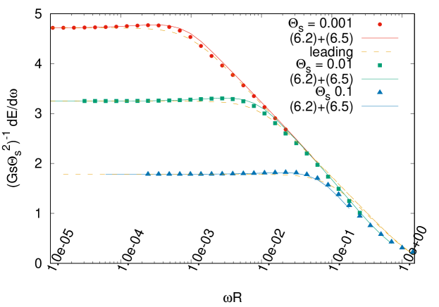
(a)

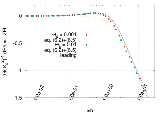
(b)

Figure 6: (a) The (reduced) graviton frequency spectrum against $\omega R$ for three values of $\Theta_{s}$. Dots represent the full spectrum, while the solid lines represent the values obtained by using the analytic approximation (6.2)+(6.5) of the amplitude. The orange-dashed lines represent the leading approximation. (b) The (reduced) graviton frequency spectrum versus $\omega b$ and with ZFL subtracted out, for two values of $\Theta_{s}$. The meaning of dots and lines is as in (a) .

In fact, by plotting the spectra against $\omega b=2\omega R/\Theta_{s}$, and by subtracting the known ZFL, we can see that they overlap, as shown in fig. 6b, where, for clarity, we limited ourselves to just two values of $\Theta_{s}=10^{-2},10^{-3}$. Here it is apparent that the spectrum, starting from its finite ZFL value at $\omega=0$, increases until $\omega b\sim 0.5$ and only at larger values of the frequency it decreases. For the “reduced” spectrum, the height of the maximum above the ZFL limit is almost independent of the (small) value of $\Theta_{s}$: its value is about 0.05.

This peculiar feature is due to the subleading terms of the amplitude. In fact the leading spectrum decreases monotonically in the whole $\omega$ range, whereas the most relevant infrared corrections to the ZFL are positive. More precisely, in sec. 6.2 we found that such corrections are logarithmic and, for the frequency spectrum, they start at $\mathcal{O}\left(\omega b\log(1/\omega b)\right)^{2}$, according to the expansion

$$\frac{1}{Gs\Theta_{s}^{2}}\frac{\mathrm{d}E^{\mathrm{GW}}}{\mathrm{d}\omega} \simeq\frac{1}{\pi}\bigg{\{}\log\frac{1}{\Theta_{s}^{2}}+1$$

$$\qquad+\frac{(b\omega)^{2}}{2}\left[\log^{2}\frac{1}{b\omega}+\mathcal{O}\left(\log\frac{1}{b\omega}\right)+\mathcal{O}\left(\Theta_{s}^{2}\right)\right]+\mathcal{O}\left(\omega^{3}\log^{3}\omega\right)\bigg{\}}\;.$$ (6.39)

As a consequence, the spectrum exhibits a maximum at a value of $b\omega$ of order unity. This is clearly seen by magnifying the deep IR region in linear scale. In fig. 7 we show the result of the full spectrum (empty and full points) at small values of $b\omega$ for $\Theta_{s}=10^{-2}$. By approaching $\omega\to 0$, they tend to the ZFL limit with vanishing slope, but their behaviour is well reproduced by eq. (6.39) (dotted violet curve) which adds to the ZFL only the $[\omega b\log(1/b\omega)]^{2}$ term.

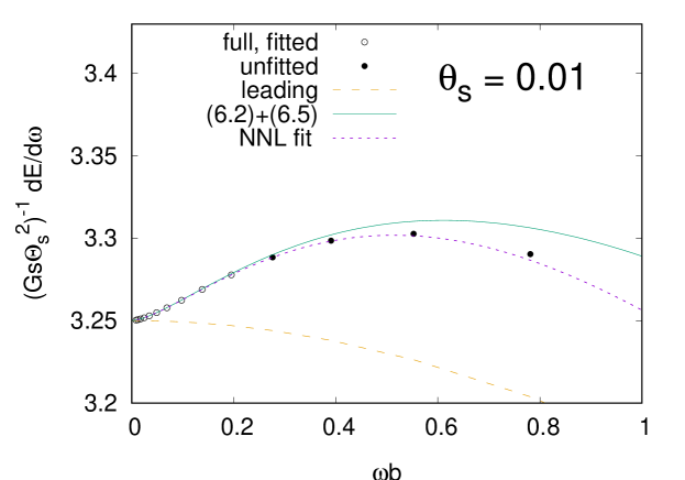
Figure 7: Behaviour of the spectrum in the soft limit $\omega b\to 0$ for $\Theta_{s}=0.01$. The full spectrum (empty and full dots) is compared with the one obtained from the analytic approximation (6.2)+(6.5) (solid green) and with the leading approximation (6.2) (dashed orange). The violet dotted line represents the function obtained by fitting the 10 leftmost data of the full spectrum.

Actually, by fitting the exact spectrum with the function
$f(b\omega)=\mathrm{ZFL}+(2\pi)^{-1}(b\omega)^{2}[a_{2}\log^{2}(1/b\omega)+a_{1}\log(1/b\omega)+a_{0}]$, (dotted violet curve) we can perfectly interpolate 10 data points within their numerical error $\mathcal{O}\left(10^{-5}\right)$, and the leading coefficient turns out to be $a_{2}=1.001\pm 10^{-3}$, i.e., well compatible with the theoretical prediction. The extrapolation of $f(b\omega)$ to larger values of the frequency is able to reproduce a few more points and to reproduce their position around the maximum (fig. 7).

In order to confirm the robustness of the $[\omega b\log(1/b\omega)]^{2}$ term, we have also fitted the same data by adding to $f(b\omega)$ possible next-to-leading terms of the form $b\omega[c_{1}\log(1/b\omega)+c_{0}]$. By asking for a best fit we have obtained very small values of $c_{0}$ and $c_{1}$, well compatible with zero, while the coefficients $a_{k}$ at $\mathcal{O}\left(b\omega\right)^{2}$ keep their values.

To summarize, we believe that our model provides strong evidence for the structure of the subleading coefficients in the soft limit of graviton emission amplitudes, with terms of order $(b\omega)^{n}\log^{m}(1/b\omega):m\leq n$. Furthermore, our model provides a reliable prediction for the “dominant” coefficients with $m=n\leq 2$.

7 Discussion

In this paper we have developed our previous work on the spectrum of gravitational waves emitted in the high-energy gravitational scattering of massless particles at leading order in the deflection angle $\Theta_{s}=\frac{4G\sqrt{s}}{b}\equiv\frac{2R}{b}$. This process can be studied either at a purely classical level [18, 19] or in a fully quantum context [20, 21, 22] with the expectation that both should agree when $\alpha_{G}\equiv\frac{Gs}{\hbar}\gg 1$ and the number of produced gravitons is large. That this is indeed the case was shown in detail in [21] (see also [22]) where the second assumption was shown to correspond to the limits $\alpha_{G}\Theta_{s}^{2}\gg 1$ and $\frac{\hbar\omega}{\sqrt{s}}\ll 1$. The overall normalization of GW spectrum $\frac{\mathrm{d}E^{\mathrm{GW}}}{\mathrm{d}\omega}$ is provided by its zero-frequency-limit (ZFL) and turns out to be of order $Gs\Theta_{s}^{2}\log(\Theta_{s}^{-2})$.

Remarkably, the spectra obtained in this “classical” limit exhibit a break in the spectrum at the characteristic “Hawking-frequency” scale $\omega_{H}\sim R^{-1}$. In other words the gravitational scattering process converts part of the initial transplanckian energy into many, deeply sub-planckian, quanta (since $\hbar/R=\sqrt{s}/\alpha_{G}\ll M_{P}$). Below such frequency the spectrum is almost flat, while above it decreases as $\omega^{-1}$ probably up to the much higher frequency $(\Theta_{s}^{2}R)^{-1}$ [18, 21].

In this work we have reconsidered carefully the low-frequency part of the spectrum, $\omega<1/R$, concentrating on some small corrections at $\omega<1/b$ which, although implicitly present in the result of refs. [18, 21], had been neglected in those previous analyses. The idea of looking more closely into this region of the spectrum was prompted by recent papers [26, 27] (see also [28]) in which the sub (and sub-sub) leading corrections to soft-graviton theorems were used to compute the corresponding sub (and sub-sub) leading corrections to the GW spectra for $\omega b\ll 1$. In those papers it was pointed out that, because of the infrared divergences of gravity in four space-time dimensions, one should expect that a straightforward expansion in powers of $\omega b$ breaks down owing to the appearance of logarithmic enhancements. In particular, an application of the naive recipes for computing those correction leads to infinities that can be attributed, ultimately, to the infinite Coulomb phase characteristic of four-dimensional physics. In refs. [26, 27] an improvement of the naive recipe at subleading level was proposed, basically amounting to replacing a logarithmically diverging time delay $\log{\tau}$ as $\tau\to\infty$ with a $\log(\omega^{-1})$. This was claimed to lead to possible observable effects, particularly on the gravitational waveform, and also possibly of the GW spectrum for some specific polarizations of the wave.

The advantage of the eikonal approach pursued in this paper is that it leads directly to a singularity-free result and to an unambiguous determination of the logarithmically enhanced contributions to the spectrum, including the determination of the scale inside the logs. The way our approach avoids the infinities is conceptually very simple. The infinite gravitational Coulomb phase, as already remarked by Weinberg in 1965 [29], comes for the exchange of soft gravitons among the initial “or” the final particles (and from singularities due to the hard-legs propagators). If the process under consideration has just 2 hard particles in the initial state and $2+N$ in the final state (with $N$ soft gravitons) the overall Coulomb phase for that process is the one of the elastic $2\to 2$ process plus the difference between the $(2+N)$-particle and the $2$-particle Coulomb phase. It is easy to see that this difference is finite but contains logs. So the Coulomb divergence becomes common to all amplitudes, factors out in impact parameter space, and cancels in all observables; but some finite logs remain and give physical effects. We have identified two such effects:

• At sub-leading order there is a correction to the ZFL of relative order $\omega b\log(\omega b)$ having interesting characteristics. It depends on the azimuthal angle $\phi$ of the wave vector w.r.t. the impact parameter (or equivalently the scattering plane) in the form of a $\pm\sin\psi$ where the the relation between $\phi$ and $\psi$ is given in (6.25), and the sign depends on the helicity (circular polarization) of the wave. This interference term appears only as a $\phi$ dependent contribution to the polarized fluxes and cancels both in their sum and upon azimuthal averaging. It also disappears if one considers the more conventional $+$ and $\times$ polarizations. All these features are in agreement with the results obtained in [26, 27] by a very different approach.

• At sub-sub-leading order there is instead a positive correction to the flux of relative order $(\omega b)^{2}\log^{2}(\omega b)$, equally shared among the two helicities. Since this is the leading correction to the zero-frequency flux (with all other corrections missing the $\log^{2}(\omega b)$ enhancement) the total flux must necessarily reach a maximum before falling down at higher $\omega$. We find (both analytically and numerically) that the position of this maximum is at $\omega b\sim 0.5$ and practically $\Theta_{s}$-independent.

It would be interesting to see how these results extend to physically more interesting cases e.g.: i) to smaller impact parameters (i.e. larger deflection angles) up to (and beyond?) the regime of inspiral; and/or, ii) to arbitrary masses and energies of the two colliding particles.

8 Acknowledgements

We would like to thank the Galileo Galilei Institute for hospitality during most of our collaboration meetings. One of us (GV) would like to thank Andrea Addazi and Massimo Bianchi for useful discussions about the relation between this work and Ref. [28], Tibault Damour for discussions about the relevance of sec. 4 to the EOB program, and Ashoke Sen for informing us of his work prior to its posting, for discussions, and for useful correspondence.