The Time-Domain Spectroscopic Survey: Radial Velocity Variability in Dwarf Carbon Stars

1 Introduction

The first carbon star was discovered by Secchi (1869) showing strong bandheads of C₂ in their optical spectra. The phrase “dwarf carbon star” would have long been considered an oxymoron since it was assumed that all carbon stars were giants AGB stars that had dredged up carbon produced in their cores which polluted their atmospheres, producing an atmospheric C/O ratio above unity. Carbon preferentially binds with oxygen to form CO. Remaining carbon can combine to form the carbon compounds C₂, CN, and CH giving rise to strong carbon molecular bandheads dominating their optical spectra.

This assumption was shown to be invalid when Dahn et al. (1977) discovered the first main-sequence carbon star, the dwarf carbon (dC) star G77-61. How could a main-sequence star have enough carbon in its atmosphere to push the C/O ratio beyond unity and create the strong carbon bandheads seen? The currently favored hypothesis is that dC stars are the products of binary mass transfer where the former AGB companion has become a white dwarf, leaving a carbon-enhanced dC primary. Indeed, about a dozen “smoking gun” systems, having composite spectra with a hot DA white dwarf component (Heber et al., 1993; Liebert et al., 1994; Green, 2013; Si et al., 2014), bolster this hypothesis.

As main sequence stars with carbon-enriched atmospheres, dC stars are probably the progenitors of the typically more luminous carbon-enhanced metal-poor (CEMP), sgCH, CH, and, perhaps, barium (Ba II) stars, which all have carbon and $s$-process enhancements (see discussion and references in Jorissen et al. 2016; De Marco & Izzard 2017). Samples of such stars have all been targets of spectroscopic radial velocity (RV) monitoring campaigns to test for binarity and characterize orbits. Sperauskas et al. (2016) recently studied the CH-like stars — giants showing CH and $s$-process abundances like CH stars, but without their halo kinematics — and showed $\sim 6$ times higher RV variability for C-rich than C-normal giants. Leiner et al. (2017) and others reported that binary interactions occur with surprising frequency, modifying the evolution of a considerable fraction of stars. Binary systems with mass transfer follow an impressive variety of evolutionary channels and may result in important and spectacular systems such as luminous red novae, Type Ia supernovae, planetary nebulae, and more. Here, we demonstrate that dCs definitively belong to the family of mass transfer binary systems.

The first dC star confirmed to be in a binary system, with a measured period of 245d, is the dC prototype G77-61 (Dearborn et al., 1986). Margon et al. (2018) recently mapped the orbit of a second system with a much shorter (3d) period. Whitehouse et al. (2018) detected radial velocity variability in 21 of 28 dC stars monitored spectroscopically with the William Herschel Telescope between 2013 and 2017.

We seek here, using multi-epoch spectroscopy of many dC stars discovered by the Sloan Digital Sky Survey (SDSS; Blanton et al., 2017), to measure the dC binary frequency, which should be near unity in this mass transfer scenario. As was the case in Whitehouse et al. (2018), our SDSS sampling lacks enough epochs to determine individual orbital parameters. However, with a significantly larger sample of 240 dC stars, we can use the distribution of radial velocity variations and Markov chain Monte Carlo methods to characterize the dC population’s separation distribution as was done by Maoz et al. (2012) and Badenes & Maoz (2012).

2 Dwarf Carbon Star Sample Selection

Dwarf carbon stars for this study were selected from the Green (2013) and Si et al. (2014) carbon star samples. Green (2013) identified carbon stars by visual inspection of single-epoch SDSS spectra compiled from the union of (1) SDSS DR7 spectra (Abazajian et al., 2009) having strong cross-correlation coefficients with the SDSS carbon star templates with (2) SDSS spectra with a DR8 pipeline class of STAR and subclass including the word carbon (Aihara et al., 2011). From within this carbon star parent sample, definitive main sequence dwarfs were selected by having significant proper motions ($\geq 3\sigma$ and 11 mas yr^-1) in the catalog of Munn et al. (2004) and/or having SDSS spectra visibly identifiable as composite DA/dC spectroscopic binaries . Si et al. (2014) selected dCs using

For our current work, which aims to measure radial velocity variability, the primary additional selection criterion was that the selected dC stars have more than one epoch of spectroscopy in the SDSS as of November 2017. The majority of such objects were intentionally targeted for a second epoch of spectroscopy with the Time Domain Spectroscopic Survey (TDSS; Morganson et al., 2015a), a subprogram of the SDSS-IV extended Baryon Acoustic Oscillation Sky Survey (eBOSS; Dawson et al., 2016) project. Within TDSS, the main single-epoch-spectroscopy (SES) program (Morganson et al., 2015b) — along with its pilot survey, dubbed SEQUELS within SDSS-III (Ruan et al., 2016) — primarily targets optical point sources (unconfirmed quasars and stars) for a first epoch of spectroscopy based on variability. However, within several “few-epoch spectroscopy” (FES) subprograms, TDSS also acquires repeat spectroscopic observations for subsets of known stars and quasars that are astrophysically interesting. The FES programs are described by MacLeod et al. (2018) and include several classes of quasars and stars, including dC stars, re-targeted to study their spectroscopic variability. For the dC FES program, we selected all 730 SDSS dC stars from Green (2013) as well as another 99 dC stars found by Si et al. (2014), totaling 829 unique dC stars

We then searched the SDSS database (using the CasJobs query tool) for spectroscopy from DR14 (Abolfathi et al., 2018) for the dC stars that have been observed in the dC FES program. We also checked the DR14 database for all dC stars in the Green (2013) sample in search of any dC stars that may have been observed more than once, but not as part of the TDSS FES program. Our final sample contains FES spectra obtained up until October 31, 2017 and spectra from DR14.

We visually inspected all spectral epochs and removed any spectra that had strong broad artifacts. The final sample for this study was 240 dCs with a total of 540 spectra within the SDSS.

Figure 1 shows the correlation between $r$ mag (Fukugita et al., 1996) and the median spectroscopic signal-to-noise ratio (S/N). The color axis is the Modified Julian Date (MJD) of each epoch, and a clear distinction can be seen between the early epochs and later epochs in regards to S/N due to the enhanced capabilities of the BOSS spectrograph.

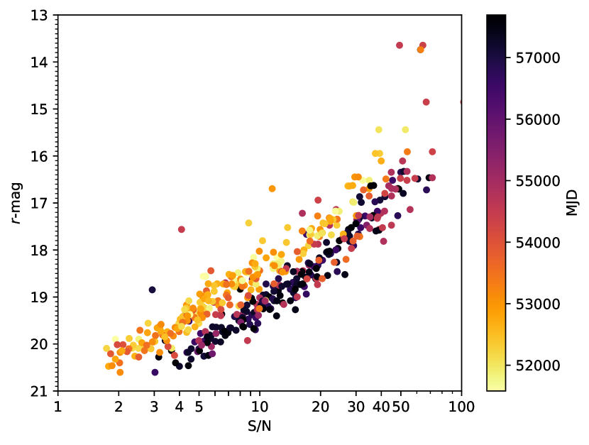
Figure 1: Optical $r$-band magnitude as a function of the median spectroscopic signal-to-noise ratio for our sample. Dots are colored by spectroscopic epoch in modified Julian days (MJD). The improved $S/N$ of later epochs (using the BOSS rather than the legacy SDSS spectrograph) is evident. As expected, there is a close correlation between brightness and $S/N$.

3 Control Sample Selection

3.1 Selection Criteria

The control sample was selected from the SDSS DR14 catalog using the properties of the dC sample as a selection criteria. The control sample criteria were as follows: (1) objects must have CLASS=STAR from the SDSS spectroscopic pipeline (2) a significant proper motion detection following the criteria of Green (2013) (3) select only stars within the 2 – 98% parameter ranges of the dC sample (i.e., total proper motion between 11 and 143 milliarcseconds yr^-1, SDSS $r$ mag between 15.9 and 20.3, and a $g-r$ color between 0.375 and 1.908 using extinction-corrected magnitudes and colors). All carbon stars (including dCs) were removed from the sample by SDSS CLASS and SUBCLASS keywords and by matching to all known dCs. Since their binary fraction is likely to be highly biased, we further removed stars originally targeted for reasons of X-ray emission or variability. Finally, all control stars were required to have a match in the Gaia DR2 data release (Gaia Collaboration et al., 2018). These criteria returned 9,822 stars that had more than one SDSS spectrum for a total of 21,820 spectra.

3.2 Property Matching

To reduce the effects of differing properties between the dC sample and the control sample, we matched the control stars to each dC by finding the normalized “distance” in a “four-property space”: $r$ mag, $g-r$ color, Gaia DR2 total proper motion, and Gaia DR2 parallax.

This distance matching was performed by creating a “normalized coordinate” out of each of the four properties. This coordinate was constructed by subtracting the minimum property value, then dividing by the maximum value for the property. This approach scales all of the values for each property into the range of $[0,1]$ based on the dC sample so that all of the properties are similarly weighted.

These coordinates were used to find the distance from each dC to all of the control stars. These distances, once sorted, give the closest matching control stars for each individual dC based on the chosen four properties. With the control sample sorted for closest matching properties to the dC sample, we drew the closest matches for each dC to create the final, property-matched control sample to analyze along the dC sample. Figure 2, compares histograms of these four properties for the dC and control samples.

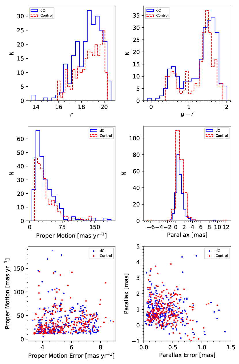
Figure 2: Comparison plot for the four properties used to match the control sample to the dC sample. The first four panels are histograms of the four properties used in the control sample matching process. The dC sample is in solid blue lines, and the control sample is in dashed red lines. Our matching process is designed to recreate the dC histograms with the control sample.

3.3 Control Sample Issues

The control sample, even given the matching process we used, is not perfect for several reasons.

(1) The SDSS stellar sample produced by a hodgepodge of different targeting programs, some of which may skew the $\Delta$RV distribution.

(2) It could be more difficult to detect binarity in the control sample because the single spectrum of an unresolved binary contains (by definition) both components. If the two components have significantly different main sequence spectral types or evolutionary stage (e.g., giant + dwarf), then one component is much more luminous than the other — similar to the dC systems we expect, which likely contain a white dwarf too cool to detect in most spectra. However, if the two components have close spectral types (e.g., a K7+M2 binary), they contribute similarly to the spectral flux. Thus, the observed velocity changes are muted because if one component is approaching, the other is receding at any epoch. There are techniques that could mitigate this issue such as attempting to fit the sum of two spectral templates to each spectrum (e.g., as proposed by El-Badry et al. 2018, but this approach would be effective only for some combinations of mass ratios and S/N.

(3) The control sample has a significantly different MJD sampling than that of the dC sample. A majority of the control sample was observed in the earliest versions of the SDSS and have $\Delta$MJDs between spectroscopic epochs on average of 100 days. Most of the dC stars have been specifically targeted by TDSS for repeat spectroscopy during SDSS-IV; so, they have a $\Delta$MJD distribution of typically 1000s of days. While this sampling does affect the range of periods our methods are sensitive to, it should not impact our results. Since we are searching for close binary systems which have large $\Delta$RVs and, therefore, short periods, the control sample’s accessible $\Delta$MJD distribution would only impede our ability to detect wide binary systems for which our sensitivity is already severely limited by the RV errors .

The first two items are observational and may diminish the discriminating power of our tests. Other intrinsic differences may complicate our analysis and interpretation of the results. For instance, we expect dC stars to have a 100% binary fraction, but a very narrow range of companion masses (all white dwarfs, therefore, strongly peaked near 0.5$\,M_{\odot}$). By contrast, the control sample has a certain binary fraction, but the distribution of companion masses in those binaries will have a wider range. The orbital properties of binaries in the control sample may also have a wider range. We expect that the dC has interacted with its (former AGB) companion (e.g., either by wind accretion or Roche lobe overflow) which sets upper (and perhaps even lower) limits on the orbital separation. The only effective limit on orbital separation in the control sample is that the pair be spatially unresolved ($\sim$$<$ $\,2\arcsec$).

4 Radial Velocity Analysis

4.1 Cross-Correlation Method

We measured radial velocity variations ($\Delta$RV) using the IRAF (Tody, 1993) package FXCOR that cross-correlates between a template and object spectrum following the methods of Tonry & Davis (1979).

Each spectrum was visually inspected to insure the S/N was sufficiently high for cross-correlation as well as to identify wavelength regions with corrupt data. We also searched for any problematic features that could affect the cross-correlation. Those objects that had corrupted regions were marked and individually run through the cross-correlation, ignoring those corrupted regions. The rest of the sample was cross-correlated in a batch, all using the same constraints and regions.

Each epoch combination’s cross-correlation function was manually inspected to check the quality of the cross-correlation. In a small ($\sim$10%) fraction of cases, the cross-correlation function is best fit manually. If the cross-correlation function could not be fit (e.g., no peak in the CCF is preferred), that epoch combination was removed from the sample.

4.2 Cross-Correlation Errors

To validate the cross-correlation process, we ran a variety of tests. The first was to verify and, if possible, minimize the reported errors from FXCOR.

To minimize uncertainties in the $\Delta$RV measurements given by the cross-correlation, we two techniques: (1) direct cross-correlation of one object against itself across different epochs and (2) cross-correlation of each epoch for one object against a SDSS C star template spectrum. For each method we also experimented with changing the regions sampled (e.g., only narrow atomic lines, excluding the carbon bands, or only including carbon bands).

We use one epoch (the early MJD) as the “template” and the other epoch (the later MJD) as the “object”. This method produces some benefits over using the usual template method: (1) This cross-correlation directly provides the $\Delta$RV shift. (3) The SDSS C star template spectrum is for AGB C stars; there are no templates for dC stars.

The second test performed was to determine if the reported values and errors from FXCOR are believable for both dC and control spectra.

FXCOR was generally able to recover the applied shift in both the dC and control samples. However, the reported errors from FXCOR generally are overestimated. By comparing each object’s FXCOR-measured shift for each of the 30 different applied shifts, we determined “multi-shift” errors for each sample as the RMS of the measured $-$ applied shift (see Figure 3).

Figure 3 presents histograms for the reported FXCOR errors and the measured “multi-shift” errors for both the dC and control samples. The top panel (a) shows how across the sample, the errors are smaller for the “multi-shift” errors than those reported by FXCOR. The bottom panel (b) displays that as FXCOR error increases, so do the “multi-shift” errors (a plausible result as spectral S/N is a key factor in the error).

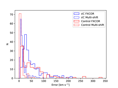
(a)

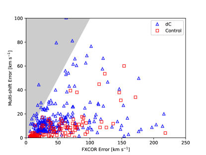
(b)

Figure 3: TOP: Histogram of reported FXCOR errors and “multi-shift” errors for both the control (red) and dC samples (blue). The errors reported by FXCOR are generally larger than the “multi-shift” errors. BOTTOM: Multi-shift vs. FXCOR-reported errors further show a poor correlation. The shaded region shows those objects where the FXCOR-reported errors are smaller; very few objects lie in this region.

Figure 4 shows the relationship between the brightness ($r$ mag) and the $\Delta$RV errors from the cross-correlation. Brightness (and by proxy S/N) determines the $\Delta$RV errors, and bluer objects tend to have smaller errors (again because these stars are usually brighter and have better S/N).

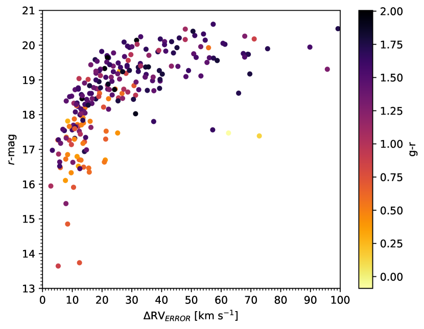
Figure 4: Optical $r$-band magnitude as a function of the radial velocity variation ($\Delta$RV) errors obtained when directly comparing two epochs of dC stars in our sample. Fainter stars have larger errors, as expected, since these tend to have poor spectroscopic $S/N$ (see Fig1). Optical $g-r$ color is denoted for each object by color.

4.3 dC and Control $\Delta$RVs

The dC and control samples were both cross-correlated using the same method. For every object, each possible combination of epochs was cross-correlated (with the earlier epoch as the template and later epoch as the object). From all possible combinations for an object, we selected the maximum $\Delta$RV for our statistical analysis.

Extremely large $\Delta$RV values (e.g., $>$600 km s^-1) in a binary with a main sequence component are suspect as in such cases we would expect extremely close orbits and strong signs of interactions and mass transfer. Therefore, any object whose $\Delta$RV was measured to be larger than this value was manually cross-correlated again and had its cross-correlation function manually fit to try and obtain a better $\Delta$RV. If the cross-correlation is unsuitable for fitting, the object was removed from the sample (this only resulted in the removal of two dCs and three control stars).

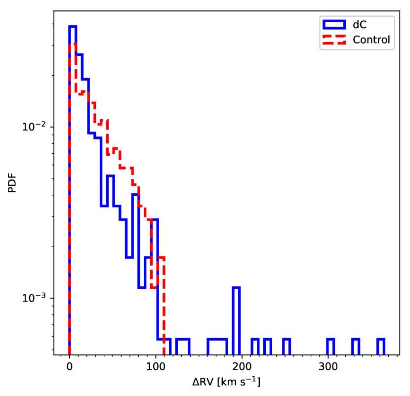
Figure 5: Normalized $\Delta$RV histogram for both of the finalized dC and control samples. The wider flaring of the base for the dC sample suggests that dCs are in close binaries.

Figure 5 is a normalized (note the log scale) histogram showing the $\Delta$RV measurements for both the dC (blue) and control (red) samples. The bins are used for each of the samples. This figure demonstrates that both samples have a central core whose width is dominated by the errors. The dC sample, however, has a tail of high $\Delta$RV systems that extends beyond this core. These systems likely represent close binary systems.

In the dC sample, these high $\Delta$RV systems those objects which display $\Delta$RV values $\geq$ 100 km s^-1. Stars that display such high $\Delta$RV values are indicative of close binary orbits. these large $\Delta$RVs were inspected by shifting the later epoch by the measured $\Delta$RV amount and visually checking to determine if features in the spectrum align.

Given that these systems display no strong signs of interaction (such as explosive variability or an accretion disk continuum emission component), few if any of the dCs are likely to have filled their Roche lobes and be transferring mass to the presumed white dwarf companion. Figure 6 shows the largest possible $\Delta$RV we would expect if the dC was filling its Roche lobe (for varying dC masses and a 0.5M_⊙ WD). Using equation 2 of Eggleton (1983), we calculate the separation for a main-sequence star of each mass to fill its Roche lobe and calculate the corresponding critical $\Delta$RV and period ($\Delta RV_{crit}$, $P_{crit}$ ) that corresponds to the Roche lobe limit. The figure suggests that while we detect dC systems that have large $\Delta$RVs; we have not detected any dCs near the Roche lobe limit .

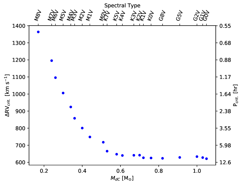
Figure 6: The maximum possible value of $\Delta$RV for a range of the expected possible dC masses with a 0.5M_⊙ WD companion. We define this maximum $\Delta$RV to be when the dC fills its Roche lobe. Using the equation of Eggleton (1983), we calculate the separation for a main-sequence star of each mass to fill its Roche lobe. Also indicated are the corresponding spectral type for each mass and the corresponding period (which is a minimum) for each of the maximum $\Delta$RVs.

Figure 7 shows spectra for the dC with one of the largest measured $\Delta$RVs. Both epochs are plotted with the early epoch in black and the late epoch in red. The top panel is of the original spectrum as observed by the SDSS. The bottom panel presents the same epochs, but the later epoch (red) has been shifted by the measured $\Delta$RV = -252 $\pm$ 15 km s^-1 amount. After this shift, the absorption features in the spectrum align confirming this measured $\Delta$RV. All pre-BOSS spectra in this figure have been smoothed by a box-car of 20 pixels, and all later spectra have been smoothed by a box-car of 15 pixels so the SDSS legacy spectra match the resolution of the new BOSS spectrograph; because otherwise, there is a spurious appearance of variability.

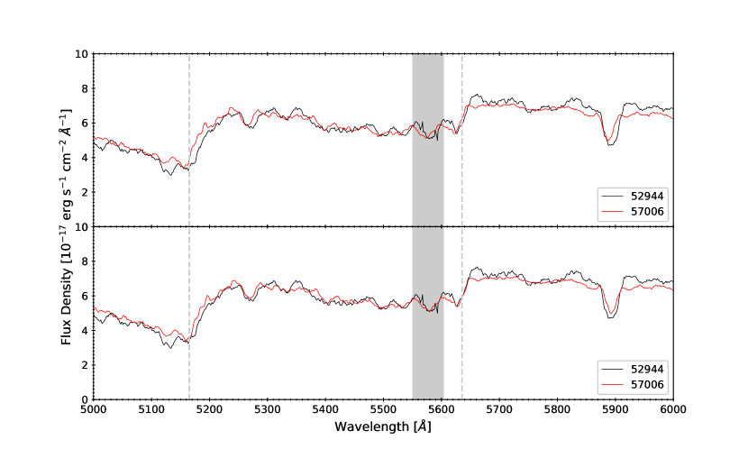
Figure 7: Smoothed spectra of both epochs for the dC with one of the largest measured $\Delta$RV, ($\alpha_{J2000}$,$\delta_{J2000}$) = (9.33893^∘, +0.20685^∘). The early epoch is in black, and the later epoch is in red. TOP: shows both epochs as measured in the SDSS. BOTTOM: shows the same spectra, but the late epoch (red) has been shifted by the measured $\Delta$RV = -252 $\pm$ 15 km s^-1. After shifting, the absorption lines clearly align between epochs confirming this $\Delta$RV and lending evidence that this dC is in a close binary orbit. The gray region is between $5550$ Å and $5604$ Å and covers the span of the OI night sky line which may contaminate the flux in that region. Locations of the C₂ bands in this wavelength range are shown.

Table 1: dC Sample Properties

Index	$\alpha_{J2000}$		$\delta_{J2000}$		$r$		$g-r$		Plate1	MJD1	FiberID1	Plate2	MJD2	FiberID2	$\Delta$RV	$\Delta$RVerror
	[Deg]		[Deg]												[km s-1]	[km s-1]
1	0.0626	28.1693	17.97	0.74	2824	54452	253	7696	57655	83	5	13
2	0.1483	-0.1875	18.74	1.42	1489	52991	156	7850	56956	704	-18	22
3	0.9212	23.9270	16.94	1.74	2801	54331	201	7665	57328	734	25	14
4	1.2380	1.1606	18.33	1.14	1490	52994	364	7862	56984	626	6	11
5	3.1909	-1.0895	19.47	1.59	687	52518	297	7863	56975	804	44	33
6	6.8651	6.6597	17.47	0.41	3106	54714	139	3106	54738	131	14	25
7	7.3310	0.7206	18.84	0.7	1087	52930	504	7855	57011	424	26	31
8	9.3389	0.2069	19.01	0.88	1495	52944	353	7868	57006	812	-252	15
9	9.9056	15.4863	18.48	0.95	419	51812	346	419	51868	346	11	26
10	10.8422	0.4788	16.72	0.55	1904	53682	495	7870	57016	562	13	8

Note. — dC property table. Each object can be identified by its SDSS plate-mjd-fiberID combination as well as its celestial coordinates. Included in this table are $r$ mag, $g-r$ color, and the measured $\Delta$RV and errors. This table is sorted on $\alpha_{J2000}$ and each dC is given an index starting at 1. This index links each dC star to the corresponding control star from the matching process. Shown here are the first 10 dC stars. A machine-readable version of the full table is available in the online journal.

Table 2: Control Sample Properties

Index	$\alpha_{J2000}$		$\delta_{J2000}$		$r$		$g-r$		Plate1	MJD1	FiberID1	Plate2	MJD2	FiberID2	$\Delta$RV	$\Delta$RVerror
	[Deg]		[Deg]												[km s-1]	[km s-1]
1	47.6415	-0.2745	17.91	0.73	2068	53386	74	7255	56597	160	1	9
2	172.5454	20.1782	18.7	1.43	3170	54859	640	3170	54907	582	-54	26
3	0.9212	23.9269	16.94	1.74	2801	54331	201	7665	57328	734	-18	19
4	35.3647	-0.2364	18.22	1.18	704	52205	234	703	52209	30	-53	19
5	170.6615	45.6529	19.65	1.57	3216	54853	143	3216	54908	156	66	55
6	6.8651	6.6597	17.47	0.41	3106	54714	139	3106	54738	131	22	11
7	10.6953	-0.6110	18.83	0.7	1905	53613	213	1905	53706	219	32	27
8	113.8683	41.4378	19.07	0.92	3658	55205	890	5941	56193	884	12	38
9	44.3177	0.9009	18.39	0.95	1512	53035	590	1512	53742	579	-2	26
10	108.2489	38.7804	16.77	0.54	2938	54503	6	2938	54526	18	3	8

Note. — Control sample property table. Each object can be identified by its SDSS plate-mjd-fiberID combination as well as its celestial coordinates. Included in this table are $r$ mag, $g-r$ color, and the measured $\Delta$RV and errors. This control table is sorted on the index which links each control star to the corresponding dC from the matching process. Shown here are the first 10 control stars that correspond to the first 10 dC stars in Table 1. A machine-readable version of the full table is available in the online journal.

Table 1 and Table 2 list the properties for the dC and control sample respectively. Only the first 10 rows for each are shown, the full machine readable tables are available online.

5 Statistical Comparison of $\Delta$RV Distributions

5.1 Anderson-Darling Test

We used a standard, two-sample Anderson-Darling (AD; Scholz & Stephens, 1987) test to determine the similarity between the dC and control $\Delta$RV distributions. From the measured dC and control $\Delta$RVs, the null hypothesis that the dC and control $\Delta$RVs are drawn from the same distribution can be rejected at the 99.95% level ($\log{p}=-3.31$).

5.2 Extreme Deconvolution

A drawback of the AD test is that it does not take measurement uncertainties into account when comparing two distributions. For example, two distributions can look dissimilar if their uncertainties are different even if their true underlying distributions are identical. To ensure that the wider $\Delta$RV observed in our dC sample in Figure 5 is not simply due to differences in the measurement uncertainties , we use the extreme deconvolution (XD) method of Bovy et al. (2011) to deconvolve the underlying distribution of our $\Delta$RV measurements. This XD method employs a Gaussian Mixture Model (GMM) to infer the underlying distribution from a set of heterogeneous, noisy observations or samples while incorporating the errors.

We tested the number of components for the XD-GMM for both the dC and control samples using the Bayesian Information Criterion (BIC) of each model. The BIC approach suggests that the dC sample is best modeled by a mixture of three Gaussians. However, the third Gaussian component for the dC population converges to a small normalization and an unphysically large width; so, we constrain the dC sample to be fit with two components. This decision allows for a central core and for a possible large $\Delta$RV tail that contains close binary systems. Table 3 lists the parameters for these fit components for both the dC and control XD-GMMs.

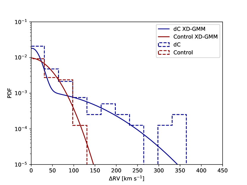
Figure 8: XD-GMM for both the dC and control samples. The histograms are the measured $\Delta$RV values from this work with the dCs in blue and the control sample in red. The smooth curves are the XD-GMM PDFs generated from the $\Delta$RV values (taking into account the $\Delta$RV errors) with the dCs in blue and the control sample in red (note the logarithmic scale). A central core is visible in both the dC and control samples, but the dC has an extended tail that extends from the core. This large $\Delta$RV tail is indicative of close binaries amid the dC population.

Table 3: XD-GMM Component Fits

Parameter	dC		Control
$\alpha_{1}$	0.688	1.00
$\mu_{1}$ [km s-1]	2.02	9.69
$\sigma_{1}$ [km s-1]	251.53	1035.82
$\alpha_{2}$	0.312	.
$\mu_{2}$ [km s-1]	2.36	.
$\sigma_{2}$ [km s-1]	12365.92	.

Note. — Values of the component fits for the XD-GMM for both the dC and control samples. Listed are the mean ($\mu$) and standard deviations ($\sigma$) of each component as well as the weights ($\alpha$; $\Sigma_{i}\alpha_{i}=1$).

Figure 8 shows the results of the XD analysis, displaying both XD-GMMs for the two samples (smooth curves) and the histogram of the measured $\Delta$RVs (both the smooth PDFs and histograms have been normalized to an integral of one). This figure demonstrates that both the dC and control samples have a core in their $\Delta$RV distribution, but the dC distribution has a much broader wide component that flares out from the core.

The width of the single component as fit to the control sample is wider than that narrow component of the dC sample. At the risk of over-interpreting this difference, we mention several effects that could contribute to this difference. First, we have used the FXCOR reported errors, which in Section 4.2 were shown to be overestimated. Since the control sample is primarily from legacy SDSS spectra with lower S/N (therefore larger errors), this overestimation is larger and may inflate the error-deconvolved core of the control distribution. Second, the single control sample fit component must accommodate the full range of single and multiple systems. Third, the narrow core of the dC sample could be real; perhaps, some fraction of dC binary orbits have actually widened due to processes related to mass transfer. Chen et al. (2018) report that some wider binaries may undergo Bondi-Hoyle-Littleton mass transfer (Edgar, 2004) and further separate since orbit-synchronized rotation of the giant star could serve as an angular momentum reservoir. However, we would still expect a narrower core for the control sample since a substantial fraction should be single stars.

It should be noted that this XD method simply uses the GMM method with errors to determine the underlying PDF as a mixture of Gaussians, but does not imply or impose any physical meaning or model on our data. However, it clearly allows us to determine that the dC sample has a tail that extends far beyond that of the control sample and is indicative of close binary systems included in the dC population.

6 Binary Orbit Simulations

While our sample lacks sufficient epochs per dC to fit individual orbits, we can use the $\Delta$RV distribution to model the separation distribution. Assuming a primitive dC mass distribution further allows us to characterize the expected period distribution of the dC sample.

Since little is known of dC orbital properties outside of G77-61, we make some physically-driven assumptions. First, we assume that the dC orbits have been circularized ($e=0$) since we expect all of them to have undergone mass transfer. Third, we assume that the WD mass distribution follows that found by Kepler et al. (2007) (i.e., a combination of four Gaussian components. The dominant component is centered on $0.58$ M_⊙ with a width of $0.047$ M_⊙). We use the distribution for the hot WD sample in Kepler et al. (2007) since they state the distribution for the cooler WDs is not reliable. We also assume a probability density function (PDF) that is uniform over $\cos{i}$ in order to determine the PDF for $\sin{i}$. Finally, since there are no known constraints on the dC mass distribution, we assume a uniform PDF over the range of 0.2$M_{\odot}$ and 1.0$M_{\odot}$, simply assuming that dCs span the same range of masses as normal main sequence stars of the same $g-r$ color distribution.

With these assumed PDFs we simulate a population of stars and sample those orbits to obtain a simulated $\Delta$RV distribution. Comparing the simulated $\Delta$RV distribution to the measured one allows the MCMC to map the separation distribution parameter space.

For the first simulation, we assumed that separations that follow a log-normal distribution with unknown mean $\mu$ and standard deviation $\sigma$, as shown in Equation 1. We placed no constraints on the model parameters, aside from those required by the log-normal PDF (i.e., $\sigma\geq 0.0$ km s^-1 ), and allowed the MCMC walkers to explore the parameter space freely.

$$f(a)=\frac{1}{a\sigma\sqrt{2\pi}}\exp{\left(-\frac{(\ln{a}-\mu)^{2}}{2\sigma^{2}}\right)}$$ (1)

We ran a MCMC for steps with 100 walkers using the Goodman & Weare (2010) algorithm. This approach allowed our walkers to explore all of the parameter space and sample the posterior of our model, which we checked for with the convergence of the chains. Figure 9 shows the resulting MCMC posterior distributions for our model parameters .

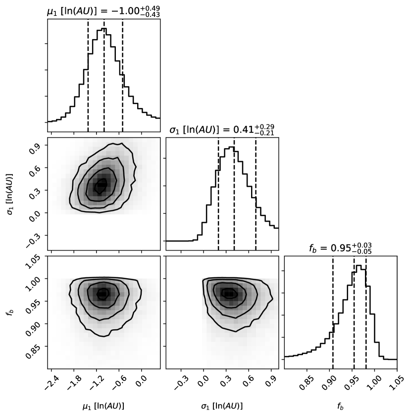
Figure 9: The posterior distributions for the model parameters ($\mu,\sigma,f_{b}$) for the unimodal log-normal distribution from the dC sample MCMC simulation. Vertical dashed lines represent the 1$\sigma$ range and the median (50${th}$ percentile). Values are the natural logarithm ($\ln{}$) of the separation in units of AU.

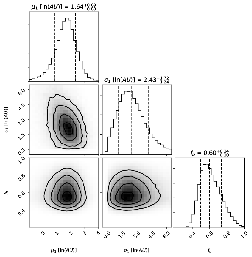
Figure 10:

The resulting separation distribution from the MCMC has a mean of 0.39 AU, a variance of 0.28 AU, and a median of 0.36 AU. These distances correspond to mean periods of 79-100 days depending on dC mass (G77-61 has a period of 245 days) and a minimum period for this distribution is on order 2.5 days (consistent with Margon et al. (2018), who found a dC with a period of 2.9 days using photometry from the Palomar Transient Factory). The separation distribution generated by our MCMC results in periods that are consistent with the periods known of individual dC systems.

However, de Kool & Green (1995) predicted that dC stars should follow a bimodal period distribution with one peak between $10^{2}-10^{3}$ days and another at $10^{3}-10^{5}$ days. Therefore, we also use our MCMC to model a bimodal mixture model (made of two log-normal separation distributions) of the form in Equation 2.

$$f(a)=\frac{\alpha}{a\sigma_{1}\sqrt{2\pi}}\exp{\left(-\frac{(\ln{a}-\mu_{1})^{2}}{2\sigma_{1}^{2}}\right)}\\ +\frac{1-\alpha}{a\sigma_{2}\sqrt{2\pi}}\exp{\left(-\frac{(\ln{a}-\mu_{2})^{2}}{2\sigma_{2}^{2}}\right)}$$ (2)

In Equation 2, $\mu_{i}$ and $\sigma_{i}$ are the same parameters as in the unimodal distribution, and $\alpha$ is the mixing parameter in this mixture model that controls how much of each distribution contributes to the total PDF. As before, we place no constraints outside of those required by the log-normal PDFs and required by the mixing parameter (i.e. $0.0\leq{}\alpha\leq{1.0}$).

This bimodal distribution MCMC simulation was run for 100,000 steps with 100 walkers. The reduction in steps is required by increased computational load when drawing from this bimodal PDF distribution. While this change does reduce the number of points in the parameter space, the MCMC walkers still mapped the posterior quite well, which we checked for with the convergence of the chains.

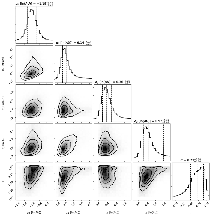
Figure 11: The posterior distributions for all five of the model parameters ($\mu_{i},\sigma_{i},\alpha$) for the bimodal mixture model of log-normal distributions from the MCMC simulations. Vertical dashed lines represent the 1$\sigma$ range and the median (50^th percentile). Values are the natural logarithm ($\ln{}$) of the separation in units of AU ($\alpha$ is a dimensionless mixture parameter).

Figure 11 shows the MCMC posterior distributions for the bimodal mixture model for all five of our model parameters . In this bimodal mixture model, the total separation distribution has a mean of 0.71 AU and a variance of 1.45 AU. This distribution gives (for the previously stated uniform dC mass range) a range of the mean period of 298-413 days and a minimum period of 1.6 days. Although the number of measured dC periods is quite sparse, the period distribution (calculated from the separation distribution) is in agreement with those few periods in the literature.

One significant improvement can be achieved by measuring dC masses via orbital fits from a follow up spectroscopy campaign. Fitting an orbit to even a few dCs will place initial physical constraints on the dC mass distribution. With a more physical and realistic dC mass distribution the models and MCMC simulations can fit a more accurate separation distribution than can be done with the currently used uniform mass distribution.

7 Balmer Emission Lines

The multi-epoch spectra present an opportunity to survey the dC sample for H$\alpha$ emission line strength and variability. Balmer line emission has been observed in dCs, and Green (2013) found that about 2.6% of dCs showed H$\alpha$ emission.

There are 10 objects with H$\alpha$ emission. Balmer line emission might be expected among dCs for several reasons: (1) coronal emission that may be a result of increased activity from spin-up during the accretion phase of the dC evolution , (2) irradiation of the dC by a hot white dwarf companion, or (3) spin-orbit coupling in a close WD/dC binary.

To explore case 1, in a related effort, we are currently analyzing Chandra observations of a small sample of dC stars to test whether their X-ray emission is consistent with dynamo rejuvenation by accretion spin-up (Green, P.J. et al. 2019, in preparation).

If the emission is from case 2, we expect to detect the WD component in the dC spectra. Indeed, all four of our DA/dCs show emission in their spectra. The remaining six of the H$\alpha$ emission line dCs are of “normal” type (i.e., no visible WD in the spectrum). H$\alpha$ emission is variable in only one normal dC and in none of the DA/dCs. Since close orbits should be involved for cases 2 and 3, we will pursue further multi-epoch spectroscopy for emission line systems.

8 Discussion

Using multi-epoch spectroscopy we have measured the radial velocity variations of a SDSS sample of dC stars. Through MCMC methods, our modeling was able to construct the separation distribution of this dC population that best recreates the observed $\Delta$RV.

We presented the best parameters for two separation models: a unimodal log-normal distribution and a bimodal mixture model of log-normal distributions. Both models result in close binary separation distributions with means less than 1 AU, corresponding to mean periods on the order of 1 year (varying depending on dC mass).

Our sample contains a handful of objects with large ($\geq$ 100 km s^-1) $\Delta$RV measurements that are indicative of close binary systems. These objects will be targeted for future spectroscopy to constrain orbital parameters thereby better characterizing the separation distribution. In addition, orbital fits will also allow us to determine the masses of the dCs assuming a WD component.

Badenes et al. (2018) analyze the RV variability of main sequence stars and report that the binary fraction is likely higher for more metal-poor stars. Carbon stars are suspected to form more easily at lower metallicity; indeed, about 20% of stars with show carbon-enhancement (e.g., Christlieb et al. 2001; Lee et al. 2013), but that frequency is increasing rapidly as metallicity decreases (Placco et al., 2014). Close binaries ($<10$ AU) also show increases in lower metallicity populations (Moe et al., 2018). The dC in G77-61 is thought to be extremely metal-poor (Gass, 1988). The measured dC $\Delta$RV distribution being wider than the control sample could in part be due both to low metallicity and to evolutionary effects since dC stars are carbon-enhanced by binary mass transfer. If the mass transfer results in inward evolution of the binary, then that should further widen the $\Delta$RV distribution for dCs. Binaries with an AGB primary can be at large separations and still, via wind-Roche lobe overflow, lose orbital angular momentum, evolve towards direct Roche lobe overflow and/or tidal friction towards a common envelope (Chen et al., 2018). Therefore, the fraction of binaries that result in mass transfer in a common envelope and a tight binary configuration may be quite large. The dC stars present a population of post mass transfer binaries that are unusually easy to identify, but may represent just a tiny fraction of such stars — those sufficiently cool and with large enough C/O to produce C₂ and/or CN bands. In some cases, the AGB evolution may have been truncated during the common envelope phase before significant carbon dredge up. A much larger space density of post mass transfer M dwarfs may remain unidentified until massive multi-epoch RV surveys become available.

Sloan 2.5-meter

References

- Abazajian et al. (2009) Abazajian, K. N., Adelman-McCarthy, J. K., Agüeros, M. A., et al. 2009, ApJS, 182, 543
- Abolfathi et al. (2018) Abolfathi, B., Aguado, D. S., Aguilar, G., et al. 2018, The Astrophysical Journal Supplement Series, 235, 42
- Aihara et al. (2011) Aihara, H., Allende Prieto, C., An, D., et al. 2011, ApJS, 193, 29
- Badenes & Maoz (2012) Badenes, C., & Maoz, D. 2012, ApJ, 749, L11
- Badenes et al. (2018) Badenes, C., Mazzola, C., Thompson, T. A., et al. 2018, ApJ, 854, 147
- Blanton et al. (2017) Blanton, M. R., Bershady, M. A., Abolfathi, B., et al. 2017, AJ, 154, 28
- Bovy et al. (2011) Bovy, J., Hogg, D. W., & Roweis, S. T. 2011, Annals of Applied Statistics, 5, arXiv:0905.2979 [stat.ME]
- Chen et al. (2018) Chen, Z., Blackman, E. G., Nordhaus, J., Frank, A., & Carroll-Nellenback, J. 2018, MNRAS, 473, 747
- Christlieb et al. (2001) Christlieb, N., Green, P. J., Wisotzki, L., & Reimers, D. 2001, A&A, 375, 366
- Dahn et al. (1977) Dahn, C. C., Liebert, J., Kron, R. G., Spinrad, H., & Hintzen, P. M. 1977, ApJ, 216, 757
- Dawson et al. (2016) Dawson, K. S., Kneib, J.-P., Percival, W. J., et al. 2016, AJ, 151, 44
- de Kool & Green (1995) de Kool, M., & Green, P. J. 1995, ApJ, 449, 236
- De Marco & Izzard (2017) De Marco, O., & Izzard, R. G. 2017, PASA, 34, e001
- Dearborn et al. (1986) Dearborn, D. S. P., Liebert, J., Aaronson, M., et al. 1986, ApJ, 300, 314
- Edgar (2004) Edgar, R. 2004, New Astronomy Reviews, 48, 843
- Eggleton (1983) Eggleton, P. P. 1983, ApJ, 268, 368
- El-Badry et al. (2018) El-Badry, K., Rix, H.-W., Ting, Y.-S., et al. 2018, MNRAS, 473, 5043
- Farihi et al. (2018) Farihi, J., Arendt, A. R., Machado, H. S., & Whitehouse, L. J. 2018, MNRAS, 477, 3801
- Foreman-Mackey (2017) Foreman-Mackey, D. 2017, corner.py: Corner plots, Astrophysics Source Code Library
- Fukugita et al. (1996) Fukugita, M., Ichikawa, T., Gunn, J. E., et al. 1996, AJ, 111, 1748
- Gaia Collaboration et al. (2018) Gaia Collaboration, Brown, A. G. A., Vallenari, A., et al. 2018, ArXiv e-prints, arXiv:1804.09365
- Gass (1988) Gass, H. 1988, Sterne und Weltraum, 27, 147
- Goodman & Weare (2010) Goodman, J., & Weare, J. 2010, Communications in Applied Mathematics and Computational Science, 5, 65
- Green (2013) Green, P. 2013, ApJ, 765, 12
- Harris et al. (2018) Harris, H. C., Dahn, C. C., Subasavage, J. P., et al. 2018, AJ, 155, 252
- Heber et al. (1993) Heber, U., Bade, N., Jordan, S., & Voges, W. 1993, A&A, 267, L31
- Hunter (2007) Hunter, J. D. 2007, Computing in Science & Engineering, 9, 90
- Jones et al. (2001–) Jones, E., Oliphant, T., Peterson, P., et al. 2001–, SciPy: Open source scientific tools for Python, [Online; accessed December 19, 2018]
- Jorissen et al. (2016) Jorissen, A., Van Eck, S., Van Winckel, H., et al. 2016, A&A, 586, A158
- Kepler et al. (2007) Kepler, S. O., Kleinman, S. J., Nitta, A., et al. 2007, MNRAS, 375, 1315
- Kleyna et al. (2002) Kleyna, J., Wilkinson, M. I., Evans, N. W., Gilmore, G., & Frayn, C. 2002, MNRAS, 330, 792
- Lee et al. (2013) Lee, Y. S., Beers, T. C., Masseron, T., et al. 2013, AJ, 146, 132
- Leiner et al. (2017) Leiner, E., Mathieu, R. D., & Geller, A. M. 2017, ApJ, 840, 67
- Liebert et al. (1994) Liebert, J., Schmidt, G. D., Lesser, M., et al. 1994, ApJ, 421, 733
- Luri et al. (2018) Luri, X., Brown, A. G. A., Sarro, L. M., et al. 2018, ArXiv e-prints, arXiv:1804.09376
- MacLeod et al. (2018) MacLeod, C. L., Green, P. J., Anderson, S. F., et al. 2018, AJ, 155, 6
- Maoz et al. (2012) Maoz, D., Badenes, C., & Bickerton, S. J. 2012, ApJ, 751, 143
- Margon et al. (2018) Margon, B., Kupfer, T., Burdge, K., et al. 2018, ApJ, 856, L2
- Moe et al. (2018) Moe, M., Kratter, K. M., & Badenes, C. 2018, ArXiv e-prints, arXiv:1808.02116 [astro-ph.SR]
- Morganson et al. (2015a) Morganson, E., Green, P. J., Anderson, S. F., et al. 2015a, ApJ, 806, 244
- Morganson et al. (2015b) —. 2015b, ApJ, 806, 244
- Munn et al. (2004) Munn, J. A., Monet, D. G., Levine, S. E., et al. 2004, AJ, 127, 3034
- Oliphant (2006) Oliphant, T. E. 2006, Guide to NumPy, Provo, UT
- Pedregosa et al. (2011) Pedregosa, F., Varoquaux, G., Gramfort, A., et al. 2011, Journal of Machine Learning Research, 12, 2825
- Placco et al. (2014) Placco, V. M., Frebel, A., Beers, T. C., & Stancliffe, R. J. 2014, ApJ, 797, 21
- Ruan et al. (2016) Ruan, J. J., Anderson, S. F., Green, P. J., et al. 2016, ApJ, 825, 137
- Scholz & Stephens (1987) Scholz, F. W., & Stephens, M. A. 1987, Journal of the American Statistical Association, 82, 918
- Secchi (1869) Secchi, A. 1869, Astronomische Nachrichten, 73, 129
- Si et al. (2014) Si, J., Luo, A., Li, Y., et al. 2014, Science China Physics, Mechanics, and Astronomy, 57, 176
- Smee et al. (2013) Smee, S. A., Gunn, J. E., Uomoto, A., et al. 2013, AJ, 146, 32
- Sperauskas et al. (2016) Sperauskas, J., Začs, L., Schuster, W. J., & Deveikis, V. 2016, ApJ, 826, 85
- The Astropy Collaboration et al. (2018) The Astropy Collaboration, Price-Whelan, A. M., Sipőcz, B. M., et al. 2018, AJ, 156, 123
- Tody (1993) Tody, D. 1993, in Astronomical Data Analysis Software and Systems II, ed. R. J. Hanisch, R. J. V. Brissenden, & J. Barnes, Vol. 52, 173
- Tonry & Davis (1979) Tonry, J., & Davis, M. 1979, AJ, 84, 1511
- Whitehouse et al. (2018) Whitehouse, L. J., Farihi, J., Green, P. J., Wilson, T. G., & Subasavage, J. P. 2018, MNRAS, 479, 3873