Generalized Ghost Dark Energy in DGP Model

Abstract

In 2000, Giorgi Dvali, Gregory Gabadadze and Massimo Porrati (Dvali et al. 2000) was proposed a new braneworld model named as DGP model, having two branches with $(\epsilon=+1)$ and $(\epsilon=-1)$. Former one $(~{}\epsilon=+1)$ known as the accelerating branch, i.e. accelerating phase of the universe can be explained without adding cosmological constant or Dark energy, whereas later one represents the decelerating branch. Here we have investigated the behavior of decelerating branch $(i.e.~{}\epsilon=-1)$ of DGP model with Generalized Ghost Dark Energy (GGDE). Aim of our study to find a stable solution of the universe in DGP model. To find a stable solution we have studied the behavior of different cosmological parameters such as Hubble parameter, equation of state (EoS) parameter and deceleration parameter with respect to scale factor. Then we have analysed the $\omega_{D}-\acute{\omega_{D}}$ to confirm no freezing region of our present study and point out thawing region. Furthermore we have checked the gradient of stability by calculating the squared sound speed. Then we extend our study to check the viability of this model under investigation through the analysis of statefinder diagnosis parameters for the present cosmological setup.

I Introduction

At the beginning of $20^{th}$ century Einstein constructed his famous general theory of relativity which can be considered as the most successful theory to understand the structure of our universe. Einstein himself believed that the universe is stationary, but after the success of Hubble’s law, expansion of the universe has been confirmed and Einstein abandoned his concept of static universe from his theory. Again in 1998 results of type Ia supernova explosion confirmed that our universe is not only expanding but also in a phase of acceleration Riess1998 ; Riess1999 ; Perlmutter1999 . This accelerated phase of the present universe is one of the most active topic of research in cosmology. Though the reason behind this expansion with an acceleration still a burning topic to the researchers. Researcher pointed out that there must be a hidden source of energy which might be responsible for this phase. This energy is termed as Dark Energy (DE) in literature. It has been assumed that $73\%$ of the total energy of the universe is dark energy having vary high negative pressure causing this acceleration. This DE model turned out to be the most promising hypothesis to explain this current phase of acceleration. The simplest model of DE is the Einstein’s cosmological constant $\Lambda$. Though Einstein abandoned this constant from his field equations to make his equations consistent with the Hubble’s law, but in order to explain the phase of acceleration of the universe this constant has to reappear in its same form but with different point of view. This constant is the key ingredient of the $\Lambda$-CDM model. In this model the equation of state has the value $\omega_{DE}=-1$ ($\omega_{DE}$ is defined as the ratio between the pressure and energy density of DE). In this scenario, the universe behaves asymptotically with a de Sitter universe. Although the $\Lambda$-CDM model is consistent very well with all observational data but it faces with the problems of fine tuning and coincidence Weinberg1989 ; Sahni2000 ; Carrall2001 ; Peebles2003 ; Padmanabhan2003 ; Tsujikawa2006 . In order to rectify the problems plagued with $\Lambda$-CDM model various dark energy models have been proposed time to time such as, chaplygin gas Kamenshchik2001 ; Bento2002 ; Zhang2006 , holographic Hsu2004 ; Li2004 , new agegraphic Cai2008 , polytropic gas Karami2009 , pilgrim Wei2012 ; Sharif2013 ; Sharif2013a . In order to justify the source of accelerating expansion (i.e. nature of DE) of the universe, two different approaches have been adopted. One way to modify the geometry part of Einstein-Hilbert action (termed as modified theories of gravity) for discussion of expansion phenomenon Sharif and Rani ; Linder ; Brans and Dicke ; Dutta and other is propose to the different forms of DE called Dynamical DE models.

Each of the dark energy models have many hidden and unique features which always make a challenging situation to the researchers. In general most of the dark energy models have required an extra degree of freedom to explain this present phase of the universe Sheykhi2009 ; Sheykhi2009a ; Sheykhi2010 ; Karami2011 ; Sheykhi2011c ; Jamil2011 . This extra term might creates inconsistency in the results. So for a desirable DE model one must resolve the problem without adopting any new degree of freedom or any kind of extra parameter. In order to do so a new model of DE known as Veneziano Ghost Dark Energy or simply Ghost Dark Energy (GDE) has been proposed by Urban2010 ; Urban2009 ; Urban2009a ; Urban2009b ; Ohta2011 . This GDE attracts the attention of researcher as its energy density ($\rho_{D}$) depends linearly on the Hubble parameter$(H)$ such as $\rho_{D}=\alpha H$, where $\alpha$ is a constant.

With the consideration of this Veneziano ghost field, the $U(1)$ problem in low energy compelling theory of Quantum Choromodynamics (QCD) has been resolved Witten1979 ; Veneziano1979 ; Rosenzweig1980 ; Nath1981 ; Kawarabayashi1980 ; K.Kawarabayashi1981 ; K.Kawarabayashi1981a . The $U(1)$ problem describes as the Lagrangian of QCD has in the massless limit, a global Chiral $U(1)$ symmetry, which does not seems to be reflected in the spacetimes of light pseudo scalar mesons. The ghost has no contribution to the vacuum energy density, which is proportional to $\Lambda^{3}_{QCD}H$, where $\Lambda_{QCD}$ is QCD mass scale and $H$ is Hubble parameter. This small vacuum energy density expect to play an important role in the evolution of universe Rong-Gen Cai . Considering GDE model above issues can be explained smoothly but GDE model faces the problem of stability Ebrahimi2011b ; CaiarXiv , which clearly indicating that the energy density does not depends on $H$ explicitly rather it depends on the higher order terms of $H$ too, which is referred as Generalized Ghost Dark Energy (GGDE) model. In GGDE model, the vacuum energy of the Ghost field can be taken as a dynamical cosmological constant F.R.Urban1 ; F.R.Urban11 ; F.R.Urban111 ; F.R.Urban1111 ; Ohta . In the ref. A.R.Zhitnitsky , the author discussed the contribution of the Veneziano QCD ghost field to the vacuum energy is not exactly of order $H$ and a sub-leading term $H^{2}$ appears due to the fact that the vacuum expectations value of the energy momentum tensor is conserved in isolation Maggiore2011 . Then the vacuum energy of the ghost field can be written as $H+O(H^{2})$, where the sub-leading term $H^{2}$ play a crucial role in the early stage of universe evolution action as the early DE Rong-Gen Cai . The density of this generalized ghost dark energy (GGDE) reads Rong-Gen Cai as,

$$\rho_{D}=\alpha H+\beta H^{2},$$ (1)

where $\alpha$ and $\beta[energy]^{2}$ are the constant parameter of the model, which should be determined.

The present work has been performed in the DGP braneworld model Gia Dvali , which was proposed by Dvali, Gabadadze and Porrati in 2000. In this braneworld scenario our universe has been considered to be brane embedded in higher dimensional spacetime. There are lot of works available in literature on higher dimensional gravity especially in brane cosmology Antoniadis ; Randal . This model indicates the existence of a $4+1$ dimensional Minkowski space, within which ordinary $3+1$ dimensional Minkowski space is embedded. In DGP Gravity, the parameter $\epsilon=\pm 1$ correspond to two branches of DGP model. The solution with $\epsilon=+1$ leads to a self accelerating branch, for this branch dark energy is no longer be required to describe the accelerated phase of the present universe Koyama(2007) . Whereas $\epsilon=-1$ corresponds to the solution for normal branch, where it has been claimed that dark energy is the only responsible of this accelerated phase of expansion of the universe Lazkozet al.2006 . To overcome this problem different investigation have been attempted to discuss DE model in DGP theory, a cosmoligical constant Lue and starkman 2004 ; Sahni and Shtanov 2003 ; Lazkoz , a quintessence perfect fluid Chimento , a scalar field Zhang or chaplygin gas Bouhmadi and HDE Wu ; Liu . Motivating from these works for different DE models we have studied of GGDE model under DGP gravity and we are able to obtain physically acceptable and stable results in favor of the current phase of the universe.

The Universe’s expansion rate can be explained by the Hubble parameter $H=\frac{\dot{a(t)}}{a(t)}$, where $a(t)$ is the cosmic scale factor of the Universe and the over dot on $a$ stands for the time derivative of it. On the other hand, the deceleration parameter $(q)$ also describes the rate of the deceleration or acceleration of the Universe,

$$q=-\frac{a\ddot{a}}{\dot{a}^{2}}=-\frac{\ddot{a}}{aH^{2}}.$$ (2)

The hubble parameter ($H$) and deceleration parameter ($q$) are well known cosmological parameters which explain the evolution of the universe. However these two parameters cannot discriminate among various DE models. In this context, Sahni et al. Sahni2003 and Alam et al. Alam2003 have introduced a new geometrical diagnostic pair $(r,s)$ known as statefinder parameter. Which can be derived using the scale factor $(a)$ and its time derivatives upto third order. The statefinder parameter is completely geometric in nature as it deduced directly from the spacetime metric. These parameters are more dependable than any other parameters to study the physical acceptability of any DE models and to distinguish between them. So the statefinder parameters can be written as,

$$r=\frac{\dddot{a}}{aH^{3}}~{}~{}{\text{and}}~{}~{}s=\frac{r-1}{3(q-\frac{1}{2})}.$$ (3)

For a flat $\Lambda CDM$ model the pair has a fixed value $\{r,s\}=\{0,1\}$.

So our present study in organised in the following manner. In Sec. II we have discussed basic mathematics of DGP braneworld model. The behavior of different cosmological parameters such as Hubble parameter, deceleration parameter and EoS parameter has been describe in Sec. III. Then we have studied $\omega_{D}-\acute{\omega_{D}}$ analysis in Sec. IV. In Sec. V we check the stability of our model. Furthermore we have described the statefinder diagnosis in Sec. VI. Finally we have concluded some of the important results in Sec. VII.

II DGP Braneworld Model

In this section we have extended our study under the braneworld scenario, the five dimensional spacetime of our universe can be realized as a 3-brane embedded spacetime. Dvali- Gabadadze-Porrati (DGP) proposed a new version of this braneworld scenario in which our four dimensional Friedman-Robertson-Walker universe embedded in five dimensional Minkowski spacetime. The usual gravitational laws in this scenario can be obtained by the addition of the action with the Einstein-Hilbert action term estimated with the brane inherent curvature. Existence of this specific term in the action is induced due to quantum corrections arising from the bulk gravity and its coupling with matter living on the brane. In this model the cosmological evolution on the brane has been described by an effective Friedman equation which includes the non-trivial bulk effects onto the brane.

So the modified Firedman equation for an isotropic and homogenous universe related to our model can be written as follows Koyama 2008 ; Li et al 2004 ; Li et al 2011

$$H^{2}-\frac{\epsilon}{r_{c}}\sqrt{H^{2}+\frac{k}{a^{2}}}=\gamma\rho-\frac{k}{a^{2}},$$ (4)

where $\gamma=\frac{8\pi G}{3}$. The total cosmic fluid energy density $\rho$ can be written as $\rho=\rho_{m}+\rho_{D}$, where $\rho_{D}$ is the energy density of DE and $\rho_{m}$ is that for DM on the brane, $k$ represents the curvature parameter, $k$ can have the values $k=-1,0,1$ corresponds to open, flat and closed universe respectively in maximally symmetric space on the brane.

Here $r_{c}=\frac{M_{pl}^{2}}{2M_{5}^{3}}=\frac{G_{5}}{2G_{4}}$ denotes the cross over scale length which can be defined as the upper limit of the length at which the universe begins to dominate by higher dimensions in late time where the Hubble parameter leads towards $H\approx\frac{1}{r_{c}}$.

In flat DGP braneworld $(k=0)$, the Friedmann eqauion of Eq. 1 reduces to

$$H^{2}-\frac{\epsilon}{r_{c}}H=\gamma(\rho_{m}+\rho_{D}).$$ (5)

Now we define the dimensionless density parameters as usual

$$\Omega_{m}=\frac{\rho_{m}}{\rho_{cr}}~{}\text{and}~{}\Omega_{D}=\frac{\rho_{D}}{\rho_{cr}}$$ (6)

where $\rho_{cr}=\frac{H^{2}}{\gamma}$, which is the critical energy density. Thus the Friedmann equation reduces to the form

$$1-\epsilon\sqrt{\Omega_{r_{c}}}=\Omega_{m}+\Omega_{D},$$ (7)

where we define-

$$\Omega_{r_{c}}=\frac{1}{H^{2}r_{c}^{2}}.$$ (8)

In this present study we have used the non interacting conservation equation for effective DE and DM can be reduced to the following forms-

$$\dot{\rho}_{D}+3H\rho_{D}\left(1+\omega_{D}\right)=0,$$ (9)

$$\dot{\rho}_{m}+3H\rho_{m}=0\Rightarrow\rho_{m}=\rho_{m0}a^{-3},$$ (10)

where $\omega_{D}=\frac{p_{D}}{\rho_{D}}$ is the equation of state parameter of DE.

Now substituting the values of $\rho_{D}$ and $\rho_{m}$ from the Eqs. (1) and (10) in the Friedmann Eq. (5), we get

$$(1-\beta\gamma)H^{2}-(\frac{\epsilon}{r_{c}}+\alpha\gamma)H=\gamma\rho_{m0}a^{-3}.$$ (11)

From the above equation, we have obtained the Hubble parameter $H(a)$ as

$$H_{\pm}=\frac{(\frac{\epsilon}{r_{c}}+\gamma\alpha)\pm\sqrt{(\frac{\epsilon}{r_{c}}+\gamma\alpha)^{2}+4\gamma(1-\gamma\beta)\rho_{m0}a^{-3}}}{2(1-\gamma\beta)}.$$ (12)

We get two values of Hubble parameter H. The expansion of Universe is denoted by $H_{+}$. Based on the observational results ignoring the later one we are continue with $H_{+}$. We use H instead of $H_{+}$ throughout our paper for simplicity.

$$H_{+}=H=\frac{(\frac{\epsilon}{r_{c}}+\gamma\alpha)+\sqrt{(\frac{\epsilon}{r_{c}}+\gamma\alpha)^{2}+4\gamma(1-\gamma\beta)\rho_{m0}a^{-3}}}{2(1-\gamma\beta)}.$$ (13)

Now we define characterised scale factor $a_{\star}$ to continue our present discussion as

$$a_{\star}\equiv\left(\frac{4\gamma\rho_{DM0}(1-\gamma\beta)}{(\frac{\epsilon}{r_{c}}+\gamma\alpha)^{2}}\right)^{\frac{1}{3}}=\left(\frac{4\Omega_{DM0}(1-\gamma\beta)}{(\epsilon\sqrt{\Omega_{r_{c0}}}+\Omega_{D0}-\gamma\beta)^{2}}\right)^{\frac{1}{3}}.$$ (14)

The transition point of the universe from the dust phase to present de Sitter phase was represents by this characteristics scale factor. Following recent observational data of Planck collaboration Planck2016 , we take the values of $\Omega_{D0}$, $\Omega_{m0}$ ,$\Omega_{r_{c0}}$ and $\beta$ to be $0.689$, $0.35$, $0.03$ and $-0.1$ respectively then we get $a_{\star}\sim 1$, this indicates that the transition takes place just at present.

II.1 Energy Density

Now we obtain the energy density of dark energy by using Eq. (13) as

$$\frac{2(1-\gamma\beta)}{(\frac{\epsilon}{r_{c}}+\gamma\alpha)}\rho_{D}=\left(1+\sqrt{1+(\frac{a_{\star}}{a})^{3}}\right)$$

$$\left[\alpha+\frac{\beta(\frac{\epsilon}{r_{c}}+\gamma\alpha)}{2(1-\gamma\beta)}\left(1+\sqrt{1+(\frac{a_{\star}}{a})^{3}}\right)\right].$$ (15)

Variation of $\rho_{D}$ with respect to scale factor $a$ has been shown in Fig. 1. From the figure it is clear that the energy density is decreasing with the expansion of the universe.

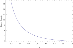
Figure 1: Variation of energy density ($\frac{2(1-\gamma\beta)\rho_{D}}{(\frac{\epsilon}{r_{c}}+\gamma\alpha)}$) with $a$.

II.2 Cosmic time evolution

Now to describe the time evolution of the Universe, we solve the Eq. (13) analytically and we get

$$\frac{(\frac{\epsilon}{r_{c}}+\gamma\alpha)}{2(1-\gamma\beta)}(t-t_{i})=-y^{3}+y^{3}\sqrt{1+y^{-3}}+\frac{3}{2}\ln y$$

$$+\ln(1+\sqrt{1+y^{-3}}),$$ (16)

where $y=\frac{a}{a_{\star}}$ and $t_{i}$ represent the initial time when $a(t_{i})=0$. Now there are two different conditions for cosmic time evolution of the universe. Firstly at early time of the universe $y\ll 1$ , the RHS of the Eq. (II.2) indicates that $\frac{(\frac{\epsilon}{r_{c}}+\gamma\alpha)}{2(1-\gamma\beta)}(t-t_{i})\approx\ 2y^{\frac{3}{2}}$, and for late time $y\gg 1$, the Eq. (II.2) indicates that $\frac{(\frac{\epsilon}{r_{c}}+\gamma\alpha)}{2(1-\gamma\beta)}(t-t_{i})\approx\frac{3}{2}\ln y$. Variation of the cosmic time evolution with respect to scale factor ‘$a$’ is shown in Fig. 2. From the figure it is clear that the cosmic time evolution is represent the present accelerated phase from early decelerating phase of the universe.

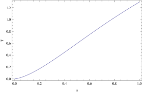
Figure 2: Variation of cosmic time evolution $T(=\frac{(\frac{\epsilon}{r_{c}}+\gamma\alpha)(t-t_{i})}{2(1-\gamma\beta)})$ with $a$.

III Cosmological Parameters

The study of cosmological parameters is an important tool to describe various properties of the universe. To describe these properties cosmological parameters includes the parameterizations of some functions, as well as some simple numbers. Actually these parameters are describing the global dynamics of the universe, i.e. the expansion rate and the curvature. Nowadays these parameters has been also studied with a great interest to describe the formation of the universe from baryons, photons, neutrinos, dark matter and dark energy. For any acceptable physical model these parameters play an important role. We have studied some of the basic parameters such as Hubble parameter, EoS parameter and deceleration parameter of our present GGDE model under DGP braneworld gravity.

III.1 Hubble Parameter

From the Eqs. (13) and (14) we observe that at early time of the universe i.e at $a\ll a_{\star}$, $H\propto a^{-\frac{3}{2}}$, which indicates the dust phase of the universe. For $a\gg a_{\star}$, i.e at late time of the universe, $H=$ constant, which denotes the entry at the de sitter phase at the later epoch. These values are perfectly right which mentioned earlier that $a_{\star}$ represents the transition point between the two epochs.

Variation of Hubble parameter of Eq. (13) with respect cosmic scale factor $(a)$ has been shown in Fig. 1. The figure clearly indicating that value of Hubble parameter is decreases with the evolution of the Universe.

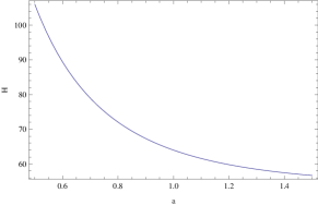
Figure 3: Variation of $H$ with $a$

III.2 EoS Parameter

Now we check the behavior of equation of state $(\omega_{D})$ parameter in this model. To evaluate the value of $(\omega_{D})$ we first take the time derivative of Eq. (13) after using Eq. (14), we arrive as

$$\frac{\dot{H}}{H^{2}}=-\frac{3}{2}\frac{(\frac{a_{\star}}{a})^{3}}{\sqrt{1+(\frac{a_{\star}}{a})^{3}}[1+\sqrt{1+(\frac{a_{\star}}{a})^{3}}]}.$$ (17)

From Eq. (9) we get

$$\omega_{D}=-\frac{\dot{\rho_{D}}}{3H\rho_{D}}-1.$$ (18)

While taking time derivative of $\rho_{D}=\alpha H+\beta H^{2}$, we find

$$\frac{\dot{\rho_{D}}}{\rho_{D}}=\frac{\alpha+2\beta H}{\alpha+\beta H}\frac{\dot{H}}{H}.$$ (19)

Hence the EoS $(\omega_{D})$ parameter for generalized ghost dark energy obtained as:

$$\omega_{D}=\left(\frac{a_{\star}}{a}\right)^{3}\left(\frac{1}{\sqrt{1+(\frac{a_{\star}}{a})^{3}}}-\frac{1}{1+\sqrt{1+(\frac{a_{\star}}{a})^{3}}}\right)$$ (20)

$$\left(\frac{\Omega_{D}+\beta\gamma[(\epsilon\sqrt{\Omega_{r_{c}}}-1)+X]}{2\Omega_{D}+\beta\gamma[(\epsilon\sqrt{\Omega_{r_{c}}}-\Omega_{D}+\beta\gamma-2)+X]}\right)-1$$

$$= \begin{cases}0,&\ a\ll a_{\star}\\ -1,&a\gg a_{\star},\end{cases}$$

where $X=(\Omega_{D}-\beta\gamma+\epsilon\sqrt{\Omega_{r_{c}}})\sqrt{1+(\frac{a_{\star}}{a})^{3}}$.

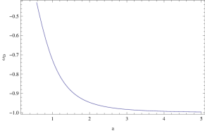
Figure 4: Variation of EoS parameter with $a$.

From this relation we can conclude that at late time the DE acts like a cosmology constant due to asymptotic behavior of $\omega_{D}$. Now we plot the figure of $\omega_{D}$ vs $a$ in Fig. 4. From the graph, we see that $\omega_{D}$ can never cross $-1$, which is similar to quintessence behavior. EoS parameter varies from zero at early time to $-1$ at late time.

Now taking time derivative of $\Omega_{D}$ we can obtain the equation of motion for dimensionless GGDE density as-

$$\dot{\Omega_{D}}=-(\Omega_{D}-\beta\gamma)(\frac{\dot{H}}{H}).$$ (21)

Using the relation $\dot{\Omega}_{D}=H\frac{d\Omega_{D}}{d\ln a}$ with Eq. (17), we obtain-

$$\frac{d\Omega_{D}}{d\ln a}=-\frac{3(\Omega_{D}-\beta\gamma)(\frac{a_{\star}}{a})^{3}}{2\sqrt{1+(\frac{a_{\star}}{a})^{3}}[1+\sqrt{1+(\frac{a_{\star}}{a})^{3}}]}.$$ (22)

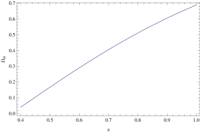
Figure 5: The evolution of $\Omega_{D}$ versus with $a$.

The extension of the dimensionless GGDE density $\Omega_{D}$ in terms of scale factor $a$ has been shown in Fig. 5. From the figure we observe that at early time $\Omega_{D}\rightarrow 0$ and at late time $\Omega_{D}\rightarrow 1$, i.e. dark energy dominated.

We can also evaluate the equation of motion for $\Omega_{r_{c}}$. In order to do so first we take time derivative of Eq. (8), and then using Eq. (17) we get

$$\frac{d\Omega_{r_{c}}}{d\ln a}=-\frac{3\Omega_{r_{c}}}{2}\frac{(\frac{a_{\star}}{a})^{3}}{\sqrt{1+(\frac{a_{\star}}{a})^{3}}[1+\sqrt{1+(\frac{a_{\star}}{a})^{3}}]}.$$ (23)

This is the equation of motion governing the evolution of GGDE under the framework of DGP Gravity.

III.3 Deceleration Parameter

Deceleration parameter is one of the most important parameter which measure expansion history of the universe. We already solved the value of $\frac{\dot{H}}{H^{2}}$ in Eq. (17), as a function of scale factor $a$ putting this value in Eq. (17), we can easily estimate the value of $q$ in terms of $a$ as

$$q = -(1+\frac{\dot{H}}{H^{2}})$$ (24)

$$= -1+\frac{3}{2}\left(\frac{a_{\star}}{a}\right)^{3}\left[\frac{1}{\sqrt{1+(\frac{a_{\star}}{a})^{3}}}-\frac{1}{1+\sqrt{1+(\frac{a_{\star}}{a})^{3}}}\right]$$

$$= \begin{cases}\frac{1}{2},&\ a\ll a_{\star}\\ -1,&a\gg a_{\star}.\end{cases}$$

Deceleration parameter $q$ decreases monotonically from $\frac{1}{2}$ to −1, which means that the expansion of the universe undergo a transition from deceleration at early epoch to acceleration at present time. Now we have plotted $q$ against scale factor for this model in Fig. 6.

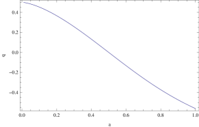
Figure 6: Variation of Deceleration parameter with $a$.

From the figure we analyze the behavior of deceleration parameter corresponding to same fixed values of constrains. We see that for increases of scale factor deceleration parameter was decreasing and decreases to more negative values. Thus the negative value of deceleration parameter demonstrates acceleration expansion of the universe, which was totally perfect for GGDE phenomenon.

IV $\omega_{D}-\acute{\omega_{D}}$ Analysis

To discuss the behavior of quintessence DE model, the $\omega_{D}-\acute{\omega_{D}}$ analysis was firstly proposed by Caldwell and LinderCaldwell2005 , where prime denotes derivative with respect to $\ln a$. They also examined the limit of quintessence model as showing thawing ($\acute{\omega_{D}}>0$ for $\omega_{D}<0$) and freezing ($\acute{\omega_{D}}<0$ for $\omega_{D}<0$) region by constructing $\omega_{D}-\acute{\omega_{D}}$ plane. The universe’s expansion in freezing region is more accelerated as compared to thawing region.

To discuss the $\omega_{D}-\acute{\omega_{D}}$ analysis for this model, we compute $\acute{\omega_{D}}$ from the Eq. (20), by taking derivative with respect to $\ln a$. Then the value of $\acute{\omega_{D}}$ is given below-

$$\acute{\omega_{D}}=\frac{1}{3}[(AB)^{2}-\frac{1}{C}AB-\frac{2\beta C}{\alpha+\beta C}B^{2}],$$ (25)

where $A=\frac{2[\alpha+\beta[\frac{\epsilon}{r_{c}}+(\alpha\gamma+\frac{\epsilon}{r_{c}})\sqrt{1+(\frac{a_{\star}}{a})^{3}}]]}{2\alpha+\beta[\frac{\epsilon}{r_{c}}+(\alpha\gamma+\frac{\epsilon}{r_{c}})\sqrt{1+(\frac{a_{\star}}{a})^{3}}-\alpha\gamma]}$,

$B=-\frac{3}{2}\frac{(\frac{a_{\star}}{a})^{3}}{\sqrt{1+(\frac{a_{\star}}{a})^{3}}[1+\sqrt{1+(\frac{a_{\star}}{a})^{3}}]}$,

$C=\frac{(\frac{\epsilon}{r_{c}}+\gamma\alpha)}{2(1-\gamma\beta)}\left(1+\sqrt{1+(\frac{a_{\star}}{a})^{3}}\right)$.

Using this value of $\acute{\omega_{D}}$ of Eq. (25) and the value of $\omega_{D}$ from Eq. (20), we plot a graph between $\omega_{D}$ and $\acute{\omega_{D}}$ given in Fig. 7. From the figure, we observe that $\acute{\omega_{D}}$ decreases as $\omega_{D}$ decreases.

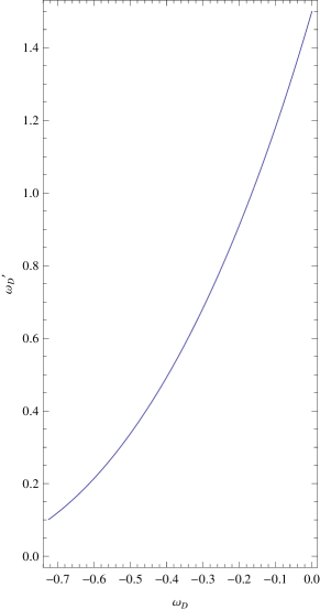
Figure 7: Variation of $\acute{\omega_{D}}$ with $\omega_{D}$

V Stability Analysis

In order to analyze the stability of GGDE model in this scenario, we extract the square speed of sound which is given by

$$v_{s}^{2}=\frac{dp}{ds}=\frac{\dot{P}}{\dot{\rho}}=\frac{\rho}{\dot{\rho}}\dot{\omega_{D}}+\omega_{D}.$$ (26)

Now putting the values of the parameters in right hand side of the above equation we get the value of the sound speed as

$$v_{s}^{2}=\frac{(\frac{a_{\star}}{a})^{3}\{\beta\gamma(1-\epsilon\sqrt{\Omega_{r_{c}}})-\Omega_{D}\}}{2\{1+(\frac{a_{\star}}{a})^{3}\}[\{\Omega_{D}-\beta\gamma(1-\epsilon\sqrt{\Omega_{r_{c}}})\}+\beta\gamma X]}.$$ (27)

We have shown the variation of sound speed $(v_{s}^{2})$ with respect to the scale factor $a$ in Fig. 8. From the figure we have observed that for GGDE model the sound speed remains positive and less than $1$ throughout cosmic evolution. Which suggest the stability of our model. Cai et al. have claimed Cai2012 that for the best fitting results sub-leading term must be negative. Following their argument we have also found that for negative value of $\beta$ the model shows stability.

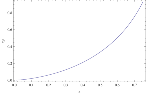
Figure 8: Variation of speed of sound with $a$.

VI Statefinder Diagnosis

To elaborate the phenomenon of GGDE in the accelerated expansion of the universe we proposed many different type of GGDE model. It is very important process to differentiate these model because of that one can decide which one provides better explanation for the current status of the universe. Since these parameters are essential, Sahni Sahni2003 introduced two new dimensionless parameters by combining the Hubble and deceleration parameter which are called statefinder parameters, are one of the most useful in geometrical tool in the sense that we can find the distance of a given GGDE model from $\Lambda CDM$ limit. Now using Eq. (17) and Eq. (24) in Eq. (3) eventually we obtain the pair of statfinder parameters as

$$r=1+3\frac{\dot{H}}{H^{2}}+\frac{\ddot{H}}{H^{3}}$$ (28)

$$= -\frac{\{(\frac{a_{\star}}{a})^{6}-16(\frac{a_{\star}}{a})^{3}-8\}-4\{1+(\frac{a_{\star}}{a})^{3}\}^{\frac{3}{2}}\{2+(\frac{a_{\star}}{a})^{3}\}}{4\{1+(\frac{a_{\star}}{a})^{3}\}^{\frac{3}{2}}\{1+\sqrt{1+(\frac{a_{\star}}{a})^{3}}\}^{2}},$$

$$s=\frac{1}{2}\frac{(\frac{a_{\star}}{a})^{6}}{(1+\sqrt{1+(\frac{a_{\star}}{a})^{3}})^{2}[1+(\frac{a_{\star}}{a})^{3}]}.$$ (29)

The evolution of the statfinder pair parameters for GGDE in the framework of DGP braneworld have been shown in Fig. 9, Fig. 10 and Fig. 11. From all of these figure we see that $r$ diverge, which corresponds to the matter dominated Universe.

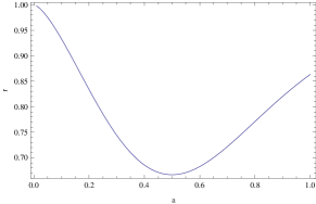
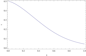
Figure 9: Variation of statefinder pair parameters with $a$.

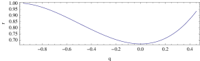
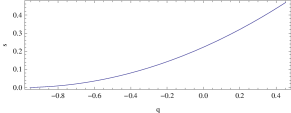
Figure 10: Variation of statfinder pair parameters with deceleration parameter $a$.

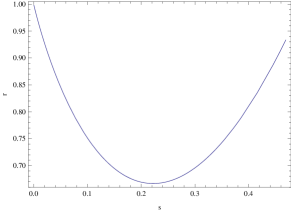
Figure 11: Variation of statfinder parameters $r$ with $s$.

VII Conclusion and Discussion

In the present study of generalized ghost dark energy model under the framework of DGP braneworld scenario, we have tried to explore several physical aspects of the model. From the observational evidences it has been confirmed that almost three-fourth part of the total energy of our universe is in the form of dark energy, which is playing very crucial role to explain the current phase of our universe. Among various available dark energy candidates, GGDE model found out to be one of the most successful model as it is free from the problem of any extra degree of freedom and it also satisfies the stability criterion. In this section we are going to summarize some of the interesting results that we have observed under this present investigation.

(i) Hubble Parameter: Recent observational results suggests that the value of Hubble parameter getting decreases with the evolution of the universe. Here we have also studied the variation of $H$ with respect to scale factor $a$ in Fig. 3 and the variation shows a monotonically decreasing nature of $H$ with $a$, which satisfies the observational results. From recent observational data of Planck collaborators Planck2016 , the value of Hubble constant can be obtained as $h=67.8\pm 0.9\ kms^{-1}\ Mpc^{-1}$. From Fig. 3 we also obtain the value of Hubble constant as $H\sim 69$ for present time (i.e. $a=1$). Which indicates that GGDE model completely agrees with the observational value of Hubble constant.

(ii)EoS Parameter: The equation of state parameter $\omega_{D}$ has been obtained for generalized ghost dark energy model in DGP braneworld scenario. At the late time, the DE acts like a cosmological constant due to asymptotic behavior of $\omega_{D}$. From the Fig. 4., we see that $\omega_{D}$ can never cross -1, which is similar to quintessence behavior. EoS parameter varies from zero at early time to $-1$ at late time. Also the dimensionless GGDE density parameter $\Omega_{D}$ in terms of scale factor $a$ is shown in Fig. 5. We see that at the early time, $\Omega_{D}\rightarrow 0$ and at late time, $\Omega_{D}\rightarrow 1$, i.e. dark energy dominated.

(iii) Deceleration Parameter: At the early epoch of evolution, the universe was dominated by matter, i.e. which caused the decelerating phase of the universe. But later on due to expansion of the universe, the phase flipped from deceleration to acceleration. This flipping caused due to domination of dark energy. Here we have studied the deceleration parameter and shows its variation with respect to the scale factor in Fig. 6, it has been observed from this plot that the signature of the deceleration parameter flipped at $a\sim 0.5$, which indicates the transition of the universe from deceleration phase to acceleration phase. This is a clear indication for physical applicability of our present form of DE as GGDE.

(iv) $\omega_{D}-\acute{\omega_{D}}$ Analysis: We have computed $\omega^{\prime}_{D}$ in terms of $a$. We have drawn $\omega^{\prime}_{D}$ versus $\omega_{D}$ in Fig. 7. In $\omega_{D}$-$\omega^{\prime}_{D}$ analysis, we have found only thawing region in that plane because $(\acute{\omega_{D}}>0$ for $\omega_{D}<0)$. So no freezing region available in our GGDE in DGP Model.

(v) Adiabatic Sound Speed ($v_{s})$: The study of adiabatic sound speed is an important parameter to describe the stability. For any stable solution we must have $0<v_{s}^{2}<1$. We have calculated the sound speed for the model GGDE and showed the variation in Fig. 8. From these figure it has been found that $v_{s}^{2}$ remains positive and within range for GGDE model.

(vi)Statefinder Parameter: Study of statefinder parameters is very essential for any physically acceptable DE model. It plays an important role to discriminate among various dark energy models. We have shown variations of the statefinder parameters in Fig. 9, Fig. 10 and Fig. 11. From Fig. 11 the variation of $r$ and $s$ in $r-s$ plane shows that the universe evolves and diverges from fixed point, i.e. from SCDM ($s\approx 1,r\approx 1$) universe (steady state) and attained least value then it increases and leads to $\Lambda CDM$ model with $(s=0,r=1)$. From this study one can discriminate between the GGDE model with other DE models.

As a final comment we can conclude that a set of physically acceptable solutions for GGDE under the framework of DGP model has been obtained. Through the analysis of various physical parameters we have found that our model is stable, which confirms that generalized ghost dark energy is one of the most acceptable form to describe accelerating phase of the present universe, whereas various studies on GDE model were unable to provide a stable solution of the universe. Again in the earlier work of Biswas et al. biswas2018 on GGDE model have showed that GGDE model provides a stable solution of the universe under the framework of FRW universe, in the similar fashion we have found that our present study on GGDE model also provides a set of stable solutions under DGP model of the universe.

References

- (1) A.G. Riess et al. (Supernova Search Team Collaboration), Astron. J. 116, 1009 (1998).
- (2) A.G. Riess, et al. Astron, J 730, 119 (2011).
- (3) S. Perlmutter et al, Astrophys. J 517, 565 (1999).
- (4) S. Weinberg, Rev. Med, Phy 61, 1 (1989).
- (5) V. Sahni and A.A. Strarobinsky, Int. J. Med. Phys. D 9, 373 (2000).
- (6) S.M. Carrall Living Rev. Rel. 4, 1 (2001).
- (7) P.J.E. Peebles and B. Ratra, Rev. Med. Phy. 75, 559 (2003).
- (8) T. Padmanabhan, Phy Rept. 380, 235 (2003).
- (9) S. Tsujikawa, Int. J. Mod. Phys. D 17, 1753 (2006).
- (10) A.Y. Kamenshchik, U. Moschella and V. Pasquier, Phys. Lett. B 511, 265 (2001).
- (11) M.C. Bento, O. Bertolami and A.A Sen, Phys. Rev. D 66, 043507 (2002).
- (12) X. Zhang, F.Q. Wu and J. Zhang, J. Cosmol. Astropart. Phys. 01, 003 (2006).
- (13) S.D.H. Hsu, Phys. Lett. B 594, 13 (2004).
- (14) M. Li, Phys. Lett. B 603, 1 (2004).
- (15) R.G. Cai, Phys. Lett. B 660, 113 (2008).
- (16) K. Karami, S. Ghaari and J. Fehri, Eur. Phys. J. C 64, 85 (2009).
- (17) H. Wei, Class. Quant. Grav. 29, 175008 (2012).
- (18) M. Sharif and A Jawad, Eur. Phys. J. C 73, 2382 (2013).
- (19) M. Sharif and A. Jawad, Eur. Phys. J. C 73, 2600 (2013).
- (20) M. Sharif and S. Rani, Astrophys. Space Sci. 345, 217 (2013); ibid. 346(2013)573.
- (21) E.V. Linder, phys.Rev D 81 127301 (2010).
- (22) C.H. Brans and R.H. Dicke, Phys. Rev. 124 425 (1961).
- (23) S. Dutta and E.N. Saridakis, J. Cosmol. Astropart. Phys. 01 013 (2010).
- (24) A. Sheykhi, Phys. Lett. B 680, 113 (2009).
- (25) A. Sheykhi, Class. Quantum Gravit. 27, 025007 (2010).
- (26) A. Sheykhi, Phys. Lett. B 681, 205 (2009).
- (27) K. Karami, et al, Gen. Relativ. Gravit. 43, 27 (2011).
- (28) M. Jamil and A. Sheykhi, Int. J. Theor. Phys. 50, 625 (2011).
- (29) A. Sheykhi and M. Jamil, Phys. Lett. B 694, 284 (2011).
- (30) F.R. Urban and A.R. Zhitnitsky, Phys. Lett. B 688, 9 (2010).
- (31) F.R. Urban and A.R. Zhitnitsky, Phys. Rev. D 80, 063001 (2009).
- (32) F.R. Urban and A.R. Zhitnitsky, J. Cosmol. Astropart. Phys. 0909, 018 (2009).
- (33) F.R. Urban and A.R. Zhitnitsky, Nucl. Phys. B 835, 135 (2010).
- (34) N. Ohta, Phys. Lett. B 695, 10 41 (2011).
- (35) E. Witten, Nucl. Phys. B 156, 269 (1979).
- (36) G. Veneziano, Nucl. phys. B 159, 213 (1979).
- (37) C. Rosenzweig, J. Schechter and C.G. Trahem, Phys. Rev. D 21, 3388 (1980).
- (38) P. Nath and R.L. Arnowitt, Phys. Rev. D 23, 473 (1981).
- (39) K. Kawarabayashi and N. Ohta, Nucl.Phys.B 175, 477 (1980).
- (40) K. Kawarabayashi and N. Ohta. Prog. Theor. phys. 66, 1789 (1981).
- (41) N.Ohta, Prog. Theor. Phys 66, 1408 (1981).
- (42) Rong-Gen Cai, Zhong-Liang Tuo and Hong-Bo Zhang, Phys. Rev. D 86, 023511 (2012).
- (43) E. Ebrahimi and A. Sheykhi, Int. J. Mod. Phys. D 20, 2369 (2011).
- (44) R.G. Cai, Z.L. Tuo and H.B. Zhang, Phys. Rev. D 84, 123501 (2010).
- (45) F.R. Urban and A.R. Zhitnitsky, Phys. Lett. B 688, 9 (2010).
- (46) F.R. Urban and A.R. Zhitnitsky, Phys, Rev. D 80, (2009) 063001.
- (47) F.R. Urban and A.R. Zhitnitsky, J. Cosmol. Astropart. Phys. 0909, 018 (2009).
- (48) F.R. Urban and A.R. Zhitnitsky, Nucl. Phys. B 835, 135 (2010).
- (49) N. Ohta, arXiv:1010.1339[astro-ph.co].
- (50) A.R. Zhitnitsky, arXiv:1112.3365.
- (51) M. Maggiore, L. Hollenstein, M. Jaccard and E. Mitsou, Phys. Lett. B 7, 04102 (2011).
- (52) G. Dvali, G. Gabadaze and M. Porrati, Phys. Lett. B 485, 208 (2000).
- (53) I.C. Bachas, D. Lewellen and T. Tomaras, Phys. Lett. B 207, 441 (1988).
- (54) L. Randall and R. Sundrum, Phys. Rev. Lett. 83, 3370 (1999).
- (55) K. Koyama, Class. Quant. Gravit. R 24, 231 (2007).
- (56) R. Lazkozet, R. Maarens and E. Majerotto, Phys. Rev. D 74, 083510 (2006).
- (57) A. Lue, G.D. Starkman, Phys. Rev. D 70, 101501 (2004).
- (58) V. Sahni, Y. Shtanov, J. Cosmol. Astropart. Phy 0311, 014 (2003).
- (59) R. Lazkoz, R. Maartens and E. Majerotto, Phys. Rev. D 74, 083510 (2006).
- (60) L.P. Chimento, R. Lazkoz, R. Maartens and I. Quiros, J. Cosmol. Astropart. Phys. 0609, 004 (2006).
- (61) H. Zhang and Z.H. Zhu, Phys. Rev. D 75, 023510 (2007).
- (62) M. Bouhmadi-Lopez and R. Lazkoz. Phys. Lett. B 654, 51 (2007).
- (63) X. Wu, R.G. Cai, Z.H. Zhu, Phys. Rev. D 77, 043502 (2008).
- (64) D.J. Liu, H. Wang and B. Yang, Phys. Lett. B 694, 6 (2010).
- (65) V. Sahni et al. J. Exp. Theor. Phys. Lett. B 77 201 (2003).
- (66) U. Alam, V. Sahni, T.D. Saini and A.A. Starobinski, Mon. Not. R. Astron. Soc. 344, 1057 (2003).
- (67) K. Koyama, Gen. Relativ. Gravit. 40 421 (2008).
- (68) M. Li Phys. Lett. B 603, 1 (2004).
- (69) M Li, X. Li, S. Wang and Y. Wang, Commun. Theor. Phys. 56, 525 (2011).
- (70) Planck Collab. 2015 Results XIII, Astron. & Astrophys. 594, A13 (2016).
- (71) R.R. Caldwell, E.V. Linder, Phys. Rev. Lett. 95, 141301 (2005).
- (72) R.G. Cai, Z.L. Tuo, Y.B. Wu, and Y.Y. Zhao, Phys. Rev. D 86, 023511 (2012).
- (73) M. Biswas, U. Debnath, S. Ghosh and B.K. Guha, arXiv:1809.04944v2.