Feedback, Dynamics, and Optimal Control in
Climate Economics

Abstract

For his work in the economics of climate change, Professor William Nordhaus was a co-recipient of the 2018 Nobel Memorial Prize for Economic Sciences. A core component of the work undertaken by Nordhaus is the Dynamic Integrated model of Climate and Economy, known as the DICE model. The DICE model is a discrete-time model with two control inputs and is primarily used in conjunction with a particular optimal control problem in order to estimate optimal pathways for reducing greenhouse gas emissions. In this paper, we provide a tutorial introduction to the DICE model and we indicate challenges and open problems of potential interest for the systems and control community.

, , , ,

1 Introduction

In the absence of deep and sustained reductions in greenhouse gas emissions, the overwhelming scientific consensus points to global warming of several degrees Celsius by 2100. Warming of this magnitude poses profound risks to both human society and natural ecosystems [46]. In response to these risks, in late 2015 at the United Nations Climate Change Conference governments around the world committed to urgent reductions in human-caused emissions of greenhouse gases, most notably carbon dioxide (CO₂), in order to limit the increase in global average temperature to well below $2~{}^{\circ}$C relative to pre-industrial levels.

With global average warming of $1~{}^{\circ}$C having already been realized, constraining temperature increases below agreed target levels will require careful control of future emissions, with the Intergovernmental Panel on Climate Change (IPCC) special report on Global Warming of $1.5~{}^{\circ}$C [47] indicating that remaining below $1.5^{\circ}$C will require net-zero CO₂ emissions by about 2050. Complicating this task are large uncertainties regarding the speed and extent of warming in response to elevated atmospheric CO₂ concentrations, coupled with the need for a policy response that balances reduced economic consumption today with avoided (and discounted) economic damages of an uncertain magnitude in the future.

To quantify the damages from anthropogenic emissions of heat-trapping greenhouse gases, specifically CO₂, economists model the dynamics of climate–economy interactions using Integrated Assessment Models (IAMs), which incorporate mathematical models of phenomena from both economics and geophysical science. Possibly the first IAM in the area of climate economics was proposed by William Nordhaus in [55]. Subsequently, Nordhaus proposed the Dynamic Integrated model of Climate and Economy (DICE) in [56], with regular refinements and parameter updates, such as [58, 59, 60, 62, 64]. Largely for this body of work, Nordhaus was awarded the 2018 Nobel Memorial Prize in Economic Sciences.

A central role for IAMs is to estimate the Social Cost of Carbon Dioxide (SC-CO₂), defined as the dollar value of the economic damage caused by a one metric tonne increase in CO₂ emissions to the atmosphere. The SC-CO₂ is used by governments, companies, and international finance organizations as a key quantity in all aspects of climate change mitigation and adaptation, including cost-benefit analyses, emissions trading schemes, carbon taxes, quantification of energy subsidies, and modelling the impact of climate change on financial assets, known as the value at risk [78]. The SC-CO₂ therefore underpins trillions of dollars worth of investment decisions [41].

A commonly used derivation for the SC-CO₂ solves an open-loop optimal control problem to determine economically optimal CO₂ emissions pathways. The open-loop use of IAMs for decision-making, however, disregards crucial uncertainties in both geophysical and economic models. As a consequence, current SC-CO₂ estimates range from US$11 per tonne of CO₂ to US$63 per tonne of CO₂ or higher, and hence the SC-CO₂ fails to reflect the true economic risk posed by CO₂ emissions, seriously compromising the accuracy of the SC-CO₂ as a price on carbon for the purposes of climate change mitigation and adaptation [42, 66, 68].

The IAM community presently pre-dominantly employs simplistic Monte Carlo-based methods to emulate the impact of parametric uncertainty on the SC-CO₂ [44], whilst recognizing that such an approach can lead to contradictory policy advice [16]. On the other hand, known resolutions to this major deficiency are computationally intractable (e.g., stochastic dynamic programming [16]) and do not easily accommodate enhanced geophysical models. At a time when governments, financial bodies [18], business [88], and even emissions-intensive industries [79, 1] are demanding a price on carbon, it is imperative that the shortcomings in quantifying uncertainty in SC-CO₂ estimates be rectified. Indeed, this is considered to be a problem of the utmost importance [15, 53, 41, 75].

Our contribution in this paper is three-fold. First, we provide a complete and replicable specification of the DICE model, with accompanying code available for download at [21]. Second, we summarize some of our recent work and update the numerical results to account for updated parameters released by Nordhaus in 2016 [62]. Third, we indicate challenges and open problems of potential interest for the systems and control community.

The paper is organized as follows. Section 2 provides a tutorial description of the DICE model and of its usage in the context of computing the Social Cost of Carbon Dioxide. Section 3 describes the benefits of receding horizon control for the DICE model both as a numerical solution technique and as a way to investigate the impact of parametric uncertainty. Section 4 considers the impact of placing constraints on the atmospheric temperature and mitigation rate constraints. Section 5 indicates potential challenges and opportunities of particular relevance for the systems and control community. Section 6 provides some brief concluding remarks.

2 The DICE Model and Methodology

There are three dominant IAMs used for the calculation of the Social Cost of Carbon Dioxide [44, 8]: the previously mentioned DICE [64, 60], Policy Analysis of the Greenhouse Effect (PAGE) [40], and Climate Framework for Uncertainty, Negotiation, and Distribution (FUND) [6]. As we will describe below, the DICE model and methodology consists of an optimal control problem for a discrete time nonlinear system. A brief description of PAGE and FUND is provided in Section 2.9.

2.1 DICE Dynamics

It should be noted that there exist different open-source implementations of DICE. While Nordhaus maintains an open-source GAMS implementation [63], a subset of the authors of this paper have recently published open-source DICE code that runs in Matlab [49] and [21] (see also [20]).

It is important to note at the outset that there is not a definitive statement of the DICE model. Rather, there are two primary sources in the form of a user’s manual [64] (updated in [61]) and the available code itself (both the manual and the code are available at [63]). Additional explanations and, occasionally, equations can be found in various other sources including [60, 62]. However, these sources are not consistent with each other and, in fact, the specification in [64] is incomplete. Furthermore, there are some minor inconsistencies between text and equations in [64]. For completeness, and with the aim of presenting the DICE model and methodology in a way that can be independently implemented, we necessarily deviate from [64] and [63]. However, the subsequent impact on the numerical results when using the default parameters (included in the Appendices) is not significant.

One further note before proceeding to the model description: while the most recent version of the model is DICE2016 (as used in, for example, [62]), the previous version of the model, DICE2013, has been widely used in the literature. Importantly, the move from DICE2013 to DICE2016 involves essentially no structural changes. Rather, the model update involves updates on initial conditions and most of the model parameters. For ease of reference, we provide initial conditions and model parameters for both DICE2013 and DICE2016 in the appendices. The Matlab DICE code [21, 49] implements both parameter sets.

Figure 1: Block Diagram of DICE.

$$T(i+1) =\Phi_{T}T(i)+B_{T}\left(F_{2\times}\log_{2}\left(\tfrac{M_{\rm AT}(i)}{M_{\rm AT,1750}}\right)+F_{\rm EX}(i)\right),$$ (CLI)

$$M(i+1) =\Phi_{M}M(i)+B_{M}\left(\sigma(i)(1-\mu(i))A(i)K(i)^{\gamma}L(i)^{1-\gamma}+E_{\rm Land}(i)\right),$$ (CAR)

$$K(i+1) =\Phi_{K}K(i)+\Delta\left(\frac{1}{1+a_{2}\,T_{\rm AT}(i)^{a_{3}}}\right)\left(1-\theta_{1}(i)\mu(i)^{\theta_{2}}\right)A(i)K(i)^{\gamma}L(i)^{1-\gamma}s(i),$$ (CAP)

$$L(i+1) =L(i)\left(\frac{{\color[rgb]{0,0,0}1+}L_{a}}{{\color[rgb]{0,0,0}1+}L(i)}\right)^{\ell_{g}},$$ (POP)

$$A(i+1) =\frac{A(i)}{1-g_{A}\exp(-\delta_{A}\Delta(i-1))},$$ (TFP)

$$\sigma(i+1) =\sigma(i)\exp\left(-g_{\sigma}(1-\delta_{\sigma})^{\Delta(i-1)}\Delta\right),$$ (EI)

The dynamics of the DICE IAM [64] are given by equations (CLI)–(EI) and the inter-relationships shown in Figure 1. Note that the equation labels are descriptive, with (CLI) describing the climate (or temperature) dynamics; (CAR) describing the carbon cycle dynamics; (CAP) describing capital (or economic) dynamics; (POP) providing population dynamics; (TFP) giving the dynamics of total factor productivity; and (EI) describing the emissions intensity of economic activity.

We describe each of the modeling blocks in Figure 1 in Sections 2.2–2.6 below. Here, however, we note that the model is nonlinear and time-varying. The model assumes two control inputs: the savings rate $s$ and the mitigation or abatement rate $\mu$. The first of these we describe more fully in Section 2.3. The latter is the rate at which mitigation of industrial carbon dioxide emissions occurs.

The model uses a time-step of 5 years, starting in the year 2015 for DICE2016 (or 2010 for DICE2013). Take the discrete time index $i\in\mathbb{N}$, the sampling rate $\Delta=5$, and the initial time $t_{0}=2015$ (or 2010) so that

$$t=t_{0}+\Delta\cdot(i-1)$$ (1)

and hence $t\in\{2015,2020,2025,\ldots\}$.

2.2 DICE “Exogenous” States

The states for population $L$, total factor productivity $A$ (which is a measure of technological progress), and carbon intensity of economic activity $\sigma$, are frequently referred to as “exogenous variables”. This is due to the fact that they are not influenced by the states for climate, carbon, or capital, which are frequently referred to as “endogenous variables” (see Figure 1).

As mentioned, there are some inconsistencies in the published literature with regards to the form of these inputs. For the sake of completeness and to remain close to the numerical results generated by [63], we present and use the exogenous states as defined in [63]. Background information on the parameters and functional form of these expressions can be found in [57], [58], and [64].

The population model (POP) is referred to as the Hassell Model [39]. Total factor productivity (TFP) yields a logistic-type function; i.e., the total factor productivity is monotonically increasing with a decreasing growth rate. Carbon intensity of economic activity (EI) is similar to total factor productivity in that it is a monotonically decreasing function with a decreasing decrease rate. The quantities $L(1)=L_{0}$ and $A(1)=A_{0}$ are prescribed initial conditions for the global population and total factor productivity in the base year.

An estimate for the initial emissions intensity of economic activity $\sigma(1)=\sigma_{0}$ can be calculated as the ratio of global industrial emissions to global economic output. The estimate of $\sigma_{0}$ can be further refined by estimating the mitigation rate in the base year. In other words, with base year emissions $e_{0}$, base year economic output $q_{0}$, and an estimated base year mitigation rate $\mu_{0}$, we can estimate $\sigma_{0}=\frac{e_{0}}{q_{0}(1-\mu_{0})}$.

An estimate of the cost of mitigation efforts is given by

$$\theta_{1}(i)=\frac{p_{b}}{1000\cdot\theta_{2}}(1-\delta_{pb})^{i-1}\cdot\sigma(i).$$ (2)

Here, $p_{b}$ represents the price of a backstop technology that can remove carbon dioxide from the atmosphere. Note that this equation embeds the assumption that the cost of such technology will decrease over time (since $\delta_{pb}\in(0,1)$) and will be proportional to the emissions intensity of economic activity.

The remaining two exogenous signals are given by

$$F_{\rm EX}(i) =f_{0}+\min\left\{f_{1}-f_{0},\frac{f_{1}-f_{0}}{t_{f}}(i-1)\right\},$$ (3)

$$E_{\rm Land}(i) =E_{L0}\cdot(1-\delta_{EL})^{i-1}.$$ (4)

The signals $F_{\rm EX}$ and $E_{\rm Land}$ are estimates of the effect of greenhouse gases other than carbon dioxide and the emissions due to land use changes, respectively.

Numerical values for all parameters can be found in the appendix as well as in the accompanying code [20].

2.3 Economic Model

We now turn to the economic component of the DICE integrated assessment model. In summary, the DICE model assumes a single global economic “capital”. Capital depreciates and is replenished by investment. The amount available to invest is some fraction of the net economic output which can be derived from the gross economic output. This is a standard economic growth model (see [2] for a comprehensive treatment of such models).

Gross economic output is the product of three terms; the total factor productivity $A$; capital $K$; and labor $L$ approximated by the global population. Additionally, capital and labor contribute at different levels given by a constant called the capital elasticity $\gamma\in[0,1]$; that is, gross economic output is given by

$$Y(i)=A(i)K(i)^{\gamma}L(i)^{1-\gamma}.$$ (5)

Note the expression corresponding to gross economic output in (CAR) (see also (20) below).

Net economic output, $Q$, is gross economic output, $Y$, reduced by two factors: 1) climate damages from rising atmospheric temperature, and 2) the cost of efforts towards mitigation:

$$Q(i) =\left(\frac{1}{1+a_{2}\,T_{\rm AT}(i)^{a_{3}}}\right)\left(1-\theta_{1}(i)\mu(i)^{\theta_{2}}\right)Y(i)$$

$$=\left(\frac{1}{1+a_{2}\,T_{\rm AT}(i)^{a_{3}}}\right)\left(1-\theta_{1}(i)\mu(i)^{\theta_{2}}\right)$$

$$\qquad\cdot A(i)K(i)^{\gamma}L(i)^{1-\gamma},$$ (6)

where $\theta_{1}$ is as defined in (2). Observe the component of net economic output in (CAP).

Net economic output can then be split between consumption and investment

$$Q(i)=C(i)+I(i)$$ (7)

and the savings rate is defined as

$$s(i)=\frac{I(i)}{Q(i)}.$$ (8)

The economic dynamics (CAP) are a capital accumulation model where capital depreciates according to

$$\Phi_{K}\doteq(1-\delta_{K})^{\Delta}$$ (9)

and is replenished by investment $I$ in the form of the product of the savings rate and net economic output; i.e.,

$$K(i+1) =\Phi_{K}K(i)+\Delta\cdot I(i)$$

$$=\Phi_{K}K(i)+\Delta\cdot Q(i)s(i)$$ (10)

and substitution of (6) into (10) yields (CAP). The savings rate $s$ is the second of the two control inputs.

2.4 The Damages Function

One of the two most contentious elements in climate economics is the specification of the damages function (see [8]). This stems from the inherent difficulty of modeling in an application where experimentation is simply not possible and the fact that rising temperatures will have different local effects. Hence, different researchers have proposed many different damage functions and levels [8]. The specific form of the damages function in DICE, as shown in (CAP), is

$$\frac{1}{1+a_{2}T_{\rm AT}(i)^{a_{3}}}$$ (11)

where, with $a_{3}=2$, the parameter $a_{2}$ is calibrated to yield a loss of 2% at 3 ^∘C (see [61] for the calibration of this and other parameters).

While a full discussion of the appropriateness of (11) is beyond the scope of this article, it is worthwhile noting that it has been vigorously argued that the above calibration of 2% loss at 3 ^∘C is unreasonably low if it is to be consistent with currently available climate science [74]. Recent efforts to empirically estimate climate damages can be found in [43].

2.5 Climate Model

The climate or temperature dynamics used in DICE are derived from a two-layer energy balance model [26, 28, 70]. In particular, a simple explicit Euler discretization is applied to an established continuous-time energy balance model to obtain (CLI). However, the implementation in [63] is not strictly causal in that the atmospheric temperature at the next time step depends on the radiative forcing at the next time step. This was previously observed in [11] and [12]. We explicitly provide the derivation of the model here for future reference. Furthermore, we note that using the causal model below, as opposed to the version in [63], has a negligible quantitative impact on the numerical results obtained using the model.

The two layers in the energy balance model are the combined atmosphere, land surface, and upper ocean (simply referred to as the atmospheric layer in what follows) and the lower ocean. We denote these two states by $T_{\rm AT}$ and $T_{\rm LO}$, respectively, and the zero reference is taken as the temperature in the year 1750. With $F(t)$ denoting the radiative forcing at the top of atmosphere due to the enhanced greenhouse effect, the (continuous-time) dynamics for these states are given by

$$C_{\rm AT}\frac{d\,T_{\rm AT}(t)}{dt} =F(t)-\lambda T_{\rm AT}(t)$$

$$\qquad-\gamma\left(T_{\rm AT}(t)-T_{\rm LO}(t)\right),$$ (12a)

$$C_{\rm LO}\frac{d\,T_{\rm LO}(t)}{dt} =\gamma\left(T_{\rm AT}(t)-T_{\rm LO}(t)\right).$$ (12b)

Here, $C_{\rm AT}$ and $C_{\rm LO}$ are the heat capacities of the atmospheric and lower ocean layers and $\gamma$ is a heat exchange coefficient. The quantity $\lambda$ is called the Equilibrium Climate Sensitivity (ECS). We discuss the ECS in Remark 1 below.

Taking an explicit Euler discretization with time-step $\Delta$ yields

$$T_{\rm AT}(i+1) =T_{\rm AT}(i)+\frac{\Delta}{C_{\rm AT}}\left(F(i)-\lambda T_{\rm AT}(i)\right.$$

$$\qquad\left.-\gamma\left(T_{\rm AT}(i)-T_{\rm LO}(i)\right)\right)$$ (13a)

$$T_{\rm LO}(i+1) =T_{\rm LO}(i)$$

$$\qquad+\frac{\Delta}{C_{\rm LO}}\left(\gamma\left(T_{\rm AT}(i)-T_{\rm LO}(i)\right)\right).$$ (13b)

With $T\doteq[T_{\rm AT}\ T_{\rm LO}]^{\top}\in\mathbb{R}^{2}$, the above can be rewritten as

$$T(i+1)=\Phi_{T}T(i)+B_{T}F(i)$$ (14)

where

$$\Phi_{T}\doteq\left[\begin{array}[]{cc}\phi_{11}&\phi_{12}\\ \phi_{21}&\phi_{22}\end{array}\right],\qquad B_{T}\doteq\left[\begin{array}[]{c}\xi_{1}\\ 0\end{array}\right]$$ (15a)

and

$$\phi_{11} =1-\frac{\Delta}{C_{\rm AT}}(\lambda+\gamma)$$ (15b)

$$\phi_{12} =\frac{\Delta\gamma}{C_{\rm AT}}$$ (15c)

$$\phi_{21} =\frac{\Delta\gamma}{C_{\rm LO}}$$ (15d)

$$\phi_{22} =1-\frac{\Delta\gamma}{C_{\rm LO}}$$ (15e)

$$\xi_{1} =\frac{\Delta}{C_{\rm AT}}\ .$$ (15f)

Atmospheric temperature rise is driven by radiative forcing, or the greenhouse effect, at the top of atmosphere and, as shown in (CLI) has a nonlinear (logarithmic) dependence on the mass of CO₂ in the atmosphere, $M_{\rm AT}$. Greenhouse gases other than CO₂ (e.g., methane, nitrous oxide, and chloroflourocarbons) contribute to the radiative forcing effect, and these are accounted for in the DICE model by the exogenously defined signal, $F_{\rm EX}$ in (3).

Remark 1 (Equilibrium Climate Sensitivity).

The parameter $\lambda$ in (12a) has a specific physical interpretation in terms of the radiative forcing and an experiment involving the doubling of atmospheric carbon. Let $F_{2\times}>0$ denote the forcing associated with equilibrium carbon doubling. Ignoring the contribution of the exogenous forcing $F_{\rm EX}$, the radiative forcing is given by

$$F(t)=F_{2\times}\log_{2}\left(\frac{M_{\rm AT}(t)}{M_{\rm AT,\,1750}}\right)$$ (16)

where $M_{\rm AT,\,1750}$ is the atmospheric mass of carbon in the year 1750. Doubling the value of atmospheric carbon from pre-industrial equilibrium yields radiative forcing of

$$F_{2\times}\log_{2}\left(\frac{2M_{\rm AT,\,1750}}{M_{\rm AT,\,1750}}\right)=F_{2\times}.$$ (17)

The Equilibrium Climate Sensitivity (ECS) is defined as the steady-state atmospheric temperature arising from a doubling of atmospheric carbon. Hence, for thermal equilibrium corresponding to a doubling of atmospheric carbon, we can combine (12a) and (16) to see that

$$F_{2\times}\log_{2}\left(\frac{2M_{\rm AT,\,1750}}{M_{\rm AT,\,1750}}\right)-\lambda\,{\rm ECS}=0$$ (18)

or $\lambda=F_{2\times}/{\rm ECS}$. In words, $\lambda$ is the ratio between the radiative forcing associated with a doubling of atmospheric carbon and the equilibrium atmospheric temperature arising from such a doubling.

2.6 Carbon Model

Similar to the temperature dynamics, (CAR) is a three-reservoir model of the global carbon cycle, with states describing the average mass of carbon in the atmosphere, $M_{\rm AT}$, the upper ocean, $M_{\rm UP}$, and the deep or lower ocean, $M_{\rm LO}$. We denote the carbon states by $M\doteq[M_{\rm AT}\ M_{\rm UP}\ M_{\rm LO}]^{\top}\in\mathbb{R}^{3}$ and the coefficients $\zeta_{ii}\in[0,1]$ give the diffusion between reservoirs. We define

$$\Phi_{M}\doteq\left[\begin{array}[]{ccc}\zeta_{11}&\zeta_{12}&0\\ \zeta_{21}&\zeta_{22}&\zeta_{23}\\ 0&\zeta_{32}&\zeta_{33}\end{array}\right],\qquad B_{M}\doteq\left[\begin{array}[]{c}\xi_{2}\\ 0\\ 0\end{array}\right].$$ (19)

The mass of atmospheric carbon is driven by CO₂ emissions due to economic activity. This occurs via a nonlinear, time-varying function as shown in (CAR), that corresponds to modeled predictions of emissions and the emissions intensity of economic activity. The additional term, $E_{\rm Land}$, captures emissions due to land use changes as given by (4) above. Hence, the total emissions are described by

$$E(i)=\\ \sigma(i)(1-\mu(i))A(i)K(i)^{\gamma}L(i)^{1-\gamma}+E_{\rm Land}(i).$$ (20)

Note that this model is conceptually similar to the three reservoir model of the Global Carbon Budget project [10]. However, the three reservoirs used by the Global Carbon Budget correspond to atmospheric, ocean, and land reservoirs.

2.7 Welfare Maximization

While the nine state, two decision variable DICE model (CLI)–(EI) can be used to predict outcomes based on externally (e.g., expert) predicted mitigation and savings rates, the inputs, and predicted outcomes, are more usually the result of solving an Optimal Control Problem (OCP). In particular, the DICE dynamics act as constraints in a social welfare maximization problem.

The social welfare $W$ is defined as the discounted sum of (time-varying) utility $U$ which depends on consumption. Consumption is derived from (7) and (8) as

$$C(i)=Q(i)(1-s(i))$$ (21)

which can be written explicitly in terms of states and inputs using (6).

The utility is taken as:

$$U(C(i),L(i))=L(i)\left(\frac{\left(\frac{C(i)}{L(i)}\right)^{1-\alpha}-1}{1-\alpha}\right),$$ (22)

where $\alpha\geq 0$ is called the elasticity of marginal utility of consumption. Note that, in the limit as $\alpha\rightarrow 1$, the utility is a logarithmic function of per capita consumption and for $\alpha\in(0,1)$, (22) behaves qualitatively like a logarithm. For $\alpha>1$, since the population $L(i)$ is bounded (as the solution of (POP)), the utility is also bounded. Indeed, denoting the upper bound on population by $\widehat{L}$ (i.e., $L(i)\leq\widehat{L}$ for all $i$), we see that

$$\lim_{(C/L)\rightarrow\infty}L\left(\frac{\left(\frac{C}{L}\right)^{1-\alpha}-1}{1-\alpha}\right)\leq-\frac{\widehat{L}}{1-\alpha}.$$

The optimal control problem of interest, maximizing the social welfare, is then given by

$$W^{\star}\doteq\max_{{\bf s},{\bf\mu}} \sum_{i=0}^{\infty}\frac{U(C(i),L(i))}{(1+\rho)^{\Delta i}}$$

$${\rm subject\ to}$$ (OCP)

$$\eqref{eq:Climate}-\eqref{eq:EI},\eqref{eq:FEX}-\eqref{eq:eland}$$

$$\mu(i),s(i)\in[0,1],\forall i\in\mathbb{N},$$

where $\rho>0$ is a prescribed discount rate.

Remark 2 (Dis. rates and soc. time preference).

It should be mentioned that the numerical value chosen for $\rho$ can have a significant impact on the results and is a subject of significant discussion. On the one hand, when analyzing capital investment decisions, discount rates of 7-9% are common [65]. On the other hand, given the extremely long time scales involved in the climate system and hence the long-term impacts of current emissions, the discount rate can also be viewed in the context of intergenerational fairness (or social time preference). Here, arguments have been made for an effective 0% discount rate [74], though rates of 1-3% are more common. In the results that follow, when not otherwise specified, we use the default value of 1.5% as in [63].

2.8 The Social Cost of Carbon Dioxide (SC-CO₂)

The Social Cost of Carbon Dioxide (SC-CO₂) in a particular year is defined as

“the decrease in aggregate consumption in that year that would change the current …value of social welfare by the same amount as a one unit increase in carbon emissions in that year.” [54]

This can be computed as shown in Figure 2 where baseline emissions and consumption (Figure 2 (a) and (b)) are defined, e.g., by solving the optimal control problem (OCP). A pulse of CO₂ emissions is then injected at a particular year (10 GtCO₂ in 2020 in Figure 2(a)) and the aggregate reduction in consumption (Figure 2(c)) over succeeding years, appropriately discounted (Figure 2(d)), is the SC-CO₂ for that year. Note the different time scales between Figure 2(a) and 2(b)-(d), which emphasizes that although industrial emissions in this scenario go to zero shortly after the year 2100, the effects of these emissions, even discounted, persist far into the future.

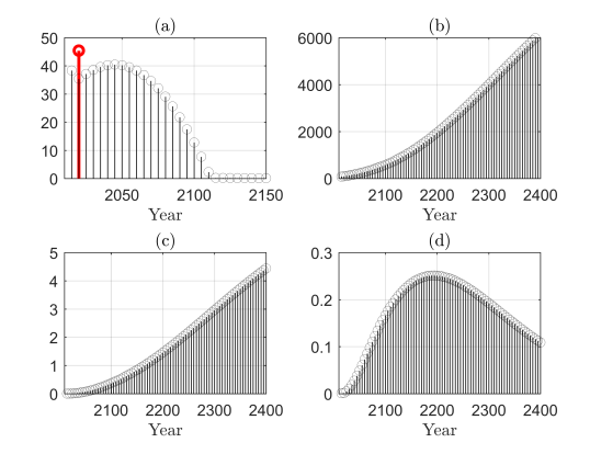
Figure 2: The Social Cost of Carbon Dioxide (SC-CO₂) computed from an emissions pulse experiment. (a) Baseline emissions and a pulse in the year 2020 (vertical axis in gigatonnes CO₂). (b) Consumption pathways resulting from the baseline and pulse emissions pathways are virtually indistinguishable (vertical axis in millions of 2010USD). (c) The difference between the baseline consumption pathway and the emissions pulse pathway (vertical axis in millions of 2010USD). (d) The 5% discounted difference between the two consumption pathways. Summing the values in this plot, and normalizing by the size of the emissions pulse, yields the SC-CO₂ for 2020.

These pulse experiments are suggestive of a sensitivity analysis and, in fact, the computation of the SC-CO₂ is given by the ratio of two Lagrange multipliers. Specifically, the Lagrange multipliers of interest are the incremental change in welfare with respect to the incremental change in emissions, $\frac{\partial W^{\star}}{\partial E(i)}$, and the incremental change in welfare with respect to the incremental change in consumption, $\frac{\partial W^{\star}}{\partial C(i)}$. The SC-CO₂ is then given by

$${\rm SC\mathchar 45\relax CO_{2}}(i) =-1000\cdot\frac{\partial W^{\star}/\partial E(i)}{\partial W^{\star}/\partial C(i)}$$

$$=-1000\cdot\frac{\partial C(i)}{\partial E(i)}.$$ (23)

Note that the factor of 1000 scales the SC-CO₂ to 2010 US dollars per tonne of CO₂, whereas consumption is in trillions of 2010 US dollars and emissions are in gigatonnes of CO₂.

As mentioned above, the discount rate $\rho$ can have a significant impact on the optimal solution and, hence, the monetary value of emissions given by the SC-CO₂. Table 1 lists the SC-CO₂ for different years and the different discount rates $\rho\in\{0.005,\,0.015,\,0,03\}$ and considering a finite horizon $N=100$. For example, the estimates SC-CO₂ for the year 2020 range from US$12.55 ($\rho=0.03$) to US$89.31 ($\rho=0.005$).

Table 1: SC-CO₂ computed for DICE2016 via [63] for selected years and different values of the discount rate $\rho$.

Year	$\rho=0.005$	$\rho=0.015$	$\rho=0.03$
2015	US$73.95	US$27.14	US$10.84
2020	US$89.31	US$32.28	US$12.54
2030	US$124.20	US$44.54	US$16.98

2.9 DICE, PAGE, and FUND

While many integrated assessment models have been proposed, the three most commonly used and cited models are DICE, PAGE, and FUND. In particular, the U.S. Interagency Working Group made use of these three models in deriving its estimates of the SC-CO₂ [44]. The PAGE model was used extensively in the Stern Review [73].

PAGE and FUND are fundamentally different models than DICE. In the economics lexicon, PAGE and FUND are “partial equilibrium models” while DICE is a “general equilibrium model”. Specifically, economic growth is an input in the former type of model, but a state (given by the evolution of $K$) in the latter. As a consequence, in solving the welfare maximization problem (OCP), DICE generates optimal emissions and consumption pathways. By contrast, such pathways must be provided as inputs to PAGE and FUND.

The PAGE model divides the world into eight regions and considers four different damages components given by sea level rise, economic damages, non-economic damages, and discontinuities. This is in contrast to DICE which considers a single global region and a single damages component. Additionally, PAGE looks to incorporate uncertainty by repeatedly drawing several parameters from probability distributions. The model is instantiated as an Excel spreadsheet and makes use of the proprietary @RISK software add-in [67] to perform the required Monte Carlo calculations.

It is important to note that PAGE takes not just economic growth (or projected Gross Domestic Product) as an input, but also climate policies (such as the mitigation rate $\mu$) as inputs. In other words, there is no optimization problem associated with the model.

FUND is similar in concept to PAGE as a partial equilibrium model, but differs in its specifics. FUND considers sixteen geographic regions and eight damages components. Furthermore, some of the damages components are dependent on both the temperature increase and the rate of temperature rise or CO₂ concentrations, while damages in DICE and PAGE are dependent solely on the temperature increase. FUND is coded in C# and is available at [5].

Given the fact that neither PAGE nor FUND involve an optimal control problem, they do not compute the SC-CO₂ as per (23), but rather do so via the pulse experiment as indicated in Figure 2.

Finally, we note that a regional variant of DICE—called RICE (Regional Integrated model of Climate and Economy)—was considered by Nordhaus in conjunction with the 2010 variant of DICE [59]. The RICE model used the same geophysical structure as previously described for DICE, but considered twelve global regions by calibrating twelve essentially independent copies of the economic model (CAP).

3 Receding Horizon Solution to DICE

As defined, (OCP) is a non-convex infinite-horizon optimal control problem and is thus difficult to solve analytically and numerically. However, from a systems-and-control perspective it is intuitive to approximate the solution to the infinite-horizon problem (OCP) by means of a receding-horizon—or model predictive control—approach. Recently the analysis of asymptotic properties of model predictive control with generic objective functionals (that do not explicitly encode a control task) has received significant attention under the label economic MPC, cf. [69, 19]. Indeed, for a very general class of problems in the undiscounted time-invariant setting, it can be shown that the receding-horizon approach yields a quantifiably accurate approximation of the infinite-horizon solution that improves as the horizon increases [29]. Extending the approximation results of [29] to include time-varying systems and discounted optimal control problems is the subject of ongoing work and some specific indications are provided at the end of this section and in Section 6.

It is worth noting that, despite the familiarity of economists with optimal control methods (e.g., [71]) and despite its significant impact on systems and control, the receding-horizon approach is still largely unknown in the economics community [34]. However, from a control point of view the welfare maximization described in (OCP) immediately suggests a receding-horizon approach for at least two reasons: One, it is conjectured that, as in the case of undiscounted optimal control problems, receding horizon control likely provides an approximate solution to the infinite horizon optimal control problem. Two, a receding horizon implementation provides a natural framework for considering robustness issues by, in particular, separating the ‘plant’ and the model of the plant used for control purposes [38]. This idea is intuitive from a control point view, yet is not the standard for climate-economy assessment. To the best of the authors’ knowledge the earliest application of a receding-horizon framework to the DICE OCP was presented in [14], which looked at the RICE model, while [85] considered the DICE model and explicitly accounted for uncertainty in emissions and temperature measurements in relation to the SC-CO₂.

Subsequently, we aim at solving (OCP) in a receding-horizon fashion to the end of computing the SC-CO₂. As mentioned before, the SC-CO₂ definition (23) can be read as a quotient of Lagrange multipliers (or adjoint states). Hence, following our development in [20], we reformulate the DICE dynamics such that the consumption $C$ and the $E$ formally can be regarded as state variables. In turn this implies that the required Lagrange multipliers / adjoints states are readily available upon solving (OCP) using state-of-the-art optimization codes.

We begin by defining the augmented state vector

$$\tilde{x}\phantom{{}_{aux}} =\begin{bmatrix}i&T&M&K&\sigma&L&A_{\rm TFP}&E_{\rm Land}&F_{\rm EX}\end{bmatrix}^{\top},$$

$$x_{aux} =\begin{bmatrix}E(i)&C(i)&\mu(i)&s(i)&W(i)\end{bmatrix}^{\top}.$$

Note that $\tilde{x}(i)\in\mathbb{R}^{12}$ collects the time index $i$, the state variables of (CLI)–(EI), and the sequences (3) and (4). The vector $x_{aux}(i)\in\mathbb{R}^{5}$ collects the emissions (20), consumption (21), inputs $\mu(i)$ and $s(i)$ at time $i$, and the extra state

$$W(i)=\sum_{j=1}^{i}\frac{U(C(j),L(j))}{(1+\rho)^{\Delta(j-1)}}$$

which is used to define the objective (social welfare). Moreover, using

$$x(i)\doteq\begin{bmatrix}\tilde{x}(i)^{\top}&x_{aux}(i)^{\top}\end{bmatrix}^{\top}$$

and the shifted input variables

$$w(i)\doteq\begin{bmatrix}\mu(i+1)&s(i+1)\end{bmatrix}^{\top},$$

we can rewrite the dynamics underlying (OCP) as follows:

$$x(i+1)=f(x(i),w(i)),\quad x(1)=v.$$ (24)

The first component of the righthand-side function $f:\mathbb{R}^{17}\times\mathbb{R}^{2}\to\mathbb{R}^{17},f=[f_{1},\dots,f_{17}]^{\top}$ is given by

$$f_{1}(x,w)\doteq x_{1}+1,$$

and the components $k=2,\dots,12$ are given by (CLI)–(EI), (3), and (4). For $k=13$ we obtain from (20)

$$E(i+1)=f_{13}(x(i),w(i))$$

$$=\Delta\left(\rule{0.0pt}{15.0pt}\sigma(i+1)(1-\mu(i+1))Y(i+1)\right.\left.+E_{\rm Land}(i+1)\rule{0.0pt}{15.0pt}\right)$$

$$=\Delta\left(\rule{0.0pt}{15.0pt}f_{8}(x(i),w(i))\cdot(1-w_{1}(i))\cdot f_{10}(x(i),w(i))\right.$$

$$\phantom{==}\qquad\cdot f_{7}(x(i),w(i))^{\gamma}\cdot\left(\tfrac{f_{9}(x(i),w(i))}{1000}\right)^{1-\gamma}$$

$$\phantom{==}\qquad\left.+\,E_{L0}\cdot(1-\delta_{EL})^{i}\rule{0.0pt}{15.0pt}\right).$$

In other words, we can rewrite the emissions explicitly as a state using (CAP)–(TFP) to expand $f_{7},f_{8},f_{9}$, and $f_{10}$. Immediately from the above, we obtain the initial emissions

$$E(1) =\Delta\left(\rule{0.0pt}{15.0pt}x_{8}(1)(1-x_{15}(1))x_{10}(1)x_{8}(1)^{\gamma}\left(\tfrac{x_{9}(1)}{1000}\right)^{1-\gamma}\right.$$

$$\phantom{==}\qquad\left.\rule{0.0pt}{15.0pt}+E_{L0}\right).$$

Similarly, we may rewrite the consumption state equation as

$$C(i+1)=f_{14}(x(i),w(i))$$

$$=\Delta\left(\frac{1-\theta_{1}(i+1)\mu(i+1)^{\theta_{2}}}{1+a_{2}\,T_{\rm AT}(i+1)^{a_{3}}}\right)Y(i+1)(1-s(i+1))$$

$$=\Delta\left(\frac{1-\theta_{1}(i+1)w_{1}(i)^{\theta_{2}}}{1+a_{2}\,f_{2}(x(i),w(i))^{a_{3}}}\right)\cdot f_{10}(x(i),w(i))$$

$$\phantom{==}\qquad\cdot f_{7}(x(i),w(i))^{\gamma}\cdot\left(\dfrac{f_{9}(x(i),w(i))}{1000}\right)^{1-\gamma}$$

$$\phantom{==}\qquad\quad\cdot(1-w_{2}(i))$$

with initial condition given by

$$C(1) =\Delta\left(\frac{1-\theta_{1}(1)x_{15}(1)^{\theta_{2}}}{1+a_{2}\,x_{2}(1)^{a_{3}}}\right)\cdot x_{10}(1)\cdot x_{8}(1)^{\gamma}$$

$$\phantom{==}\qquad\cdot\left(\tfrac{x_{8}(1)}{1000}\right)^{1-\gamma}\cdot(1-x_{16}(1)).$$

The final three states are given by

$$x_{15}(i+1) =w_{1}(i),\quad x_{15}(1)=v_{15}$$

$$x_{16}(i+1) =w_{2}(i),\quad x_{16}(1)=v_{16}$$

$$x_{17}(i+1) =x_{17}(i)+\frac{U(x_{12}(i),x_{9}(i))}{(1+\rho)^{\Delta(i-1)}},\quad x_{17}(1)=0.$$

Observe that the initial condition $x_{14}(1)=C(1)$ depends on the (unshifted) inputs at time $i=1$; i.e. it depends on $\mu(1)=x_{15}(1)$ and $s(1)=x_{16}(1)$. Likewise the initial condition $x_{13}(1)=E(1)$ depends on $\mu(1)=x_{15}(1)$.

To handle this dependence in the optimization, we introduce the auxiliary decision variable $v\in\mathbb{R}^{17}$ and the additional constraint $x(1)=v$. Now, we can summarize the equivalent (finite-horizon) reformulation of (OCP) based on the augmented dynamics (24) as follows

$$\max_{{\bf w},\,v} \ \ x_{17}(N+1)$$ (25a)

subject to

$$x(j+1) =f(x(j),w(j)),\quad j=1,\ldots,N$$ (25b)

$$x(1) =v$$ (25c)

$$v_{k} =x_{k}(1),\,k\in\{1,\dots,17\}\setminus\{15,16\}$$ (25d)

$$v_{k} \in[0,\,1],\quad k=15,16$$ (25e)

$$w(j) \in[0,\,1]\times[0,1],\quad j=1,\ldots,N.$$ (25f)

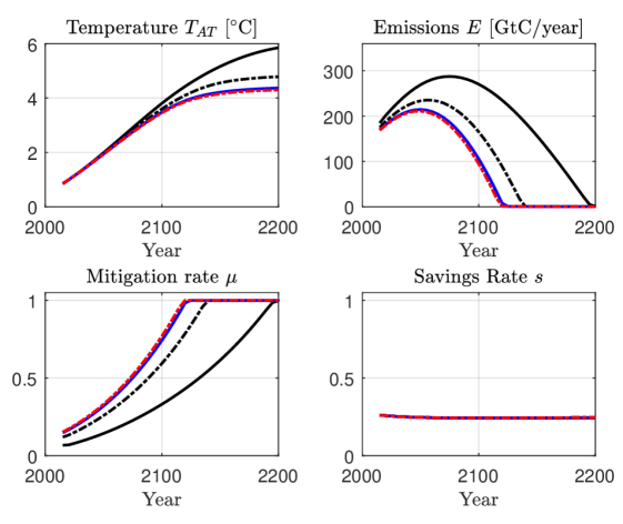
(a) Temperature, emissions, mitigation rate and savings rate.

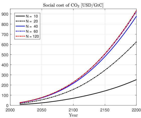
(b) Social cost of carbon dioxide.

Figure 3: Results for MPC-DICE 2016 for varying prediction horizons using Algorithm 1 with $N\in\{10,20,40,60\}$ (black, black-dashdot, blue, blue-dashdot) and the open-loop solution to (OCP) for $N=120$ (red-dashdot).

In order to obtain a receding horizon variant of the original OCP, we define a second optimization problem as follows

$$\max_{{\bf w}} \ \ x_{17}(N+1)$$ (26a)

subject to

$$x(j+1) =f(x(j),w(j)),\quad j=1,\ldots,N$$ (26b)

$$x(1) =x^{\star}(2\,|\,i-1)$$ (26c)

$$w(j) \in[0,\,1]\times[0,1],\quad j=1,\ldots,N,$$ (26d)

which differs from OCP (25) in that the initial condition $x(1)$ is available from the previous optimization via the variable $x^{\star}(2\,|\,i-1)$. This OCP is to be solved for $i=2,\dots,N_{sim}$, where $N_{sim}$ is the desired simulation horizon. Consequently, the extra decision variable $v$ is not required, since $x_{13}(1)=E^{\star}(2\,|\,i-1)$ and $x_{14}(1)=C^{\star}(2\,|\,i-1)$.

Solving either OCP (25) or OCP (26), we obtain the following data:

• The optimal state trajectory $x^{\star}(j),j=1,\dots,N+1$, which contains the savings rate and the mitigation rate as

  $$\mu^{\star}(j)=x_{15}^{\star}(j)\text{ \quad and \quad}s^{\star}(j)=x_{16}^{\star}(j).$$

• The optimal adjoint variables $\lambda^{\star}_{C}(j)$ and $\lambda^{\star}_{E}(j)$ which are given by the Lagrange multipliers associated to the equality constraints implied by the dynamics of $E(j)=x_{13}(j)$ and $C(j)=x_{14}(j)$.

Hence, the SC-CO₂ at time $j$ is obtained by

$${\rm SC\mathchar 45\relax CO_{2}}(j)=-1000\cdot\frac{\partial W/\partial E(j)}{\partial W/\partial C(j)}=-1000\cdot\frac{\lambda^{\star}_{E}(j)}{\lambda^{\star}_{C}(j)}.$$

Finally, the receding-horizon approximation of (OCP) is summarized in Algorithm 1.

Algorithm 1 MPC-DICE

1:Input: simulation horizon $N_{sim}$, prediction horizon $N$,

2:if $i==1$ then

3:Solve OCP (25)

4:Set $x(1)=x^{\star}(1|1),\lambda_{E}(1)=\lambda^{\star}_{E}(1|1),\lambda_{C}(1)=\lambda^{\star}_{C}(1|1)$.

5:for $i=2,\dots,N_{sim}$ do

6:Solve OCP (26) for $x(1)=x^{\star}(1\,|\,i-1)$.

7:Set $x(i)=x^{\star}(2\,|\,i-1),\lambda_{E}(i)=\lambda^{\star}_{E}(2\,|\,i-1),\lambda_{C}(i)=\lambda^{\star}_{C}(1\,|\,i-1)$.

8:Return $x(j)$, $\lambda_{E}(j)$ and $\lambda_{C}(j),j=0,\dots,N_{sim}$.

Remark 3 (Open source code MPC-DICE [20]).

MPC-DICE is an open-source Matlab implementation of DICE which provides parameter sets for both DICE2013 and DICE2016. Specifically, MPC-DICE provides an implementation of the receding horizon reformulation described above. It uses CasADi [4], which comes with IPOPT [82] as an NLP solver, to solve (OCP). The relatively simple CasADi syntax enables extensions of the DICE OCP, some of which we will describe in Section 4. The code is available at [21].

Figure 3 shows simulation results obtained with MPC-DICE for the 2016 parameter set for different prediction horizons $N\in\{10,20,40,60\}$ and an MPC-DICE simulation horizon $N_{sim}=40$ in comparison to the solution of (OCP) with $N=120$ of which we plot the first 40 steps. Figure 3(a) shows temperature increase, emissions as well as mitigation rate and savings rate. Figure 3(b) shows the corresponding SC-CO₂ trajectories. As one can see, for increasing prediction horizons the receding-horizon input and state trajectories both converge towards the infinite-horizon solution; approximated here by computing a long horizon solution ($N=120$). This approximation property can also be observed in Figure 3(b). Hence we conjecture that under suitable assumptions the approximation properties of MPC, which are established for time-invariant and undiscounted OCPs in [29], also hold for time-varying and discounted problems.

In fact, the theoretical results supporting this conjecture are reasonably mature where [34] shows that receding horizon control yields approximate optimal solutions for discounted problems if the turnpike property holds. Furthermore, it follows from a combination of [24] and [32] that strict dissipativity implies the turnpike property for discounted problems, provided the discount factor is sufficiently close to one. Note that the default DICE discount rate of 1.5% corresponds to a discount factor of approximately 0.985. Hence, while these results for discounted optimal control do not yet accommodate time-varying systems or cost functions, the primary difficulty lies in checking the appropriate assumptions for complicated models such as the DICE model.

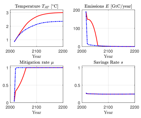
(a) Results using Algorithm 1 and the temperature increase constraint (27) with $2.36\,^{\circ}$C (blue) and $3\,^{\circ}$C (red).

(b) Results using Algorithm 1, the temperature increase constraint (27) with $3\,^{\circ}$C, the rate constraint (28a) (red) and the growth constraint (28b) (blue-dashdot).

Figure 4: Results for MPC-DICE 2016 with additional constraints.

4 State and Input Rate Constraints

The welfare maximization problem as posed in Section 2.7 considers only input magnitude constraints and the dynamics. However, in view of the reports of the IPCC, the overwhelming scientific consensus is that temperature increase should be limited to $2\,^{\circ}$C [46] and preferably to $1.5^{\circ}$C [47]. Inspection of Figure 3(a) reveals that straightforward maximization of social welfare might lead to much higher values of temperature increase in the order of $3-4\,^{\circ}$C.

This indicates that there is an inconsistency between the model (or the chosen parameters) and the scientific consensus that $2\,^{\circ}$C of warming represents a dangerous threshold. One approach to addressing this is to modify the model directly; for example by changing the climate damages function (11) to reflect the consensus that damages at $2\,^{\circ}$C are expected to be significantly higher than a loss of 0.9% of global economic output. It is also possible to consider a different welfare function that not only places a value on consumption but also values environmental “services” (such as clean air and water) [76] or accounts for the cost of adaptation to climate change [7].

A third approach, as done in [58, pp. 69–73], is to add a constraint on the temperature increase to (OCP). As mentioned in [58, pp. 69–73], the purely economic case for imposing a hard limit is somewhat unjustified as it effectively implies an infinite cost of exceeding the constraint. However, also as discussed in [58, pp. 69–73], a hard constraint can represent a tipping point where the climate damages dramatically increase, for example due to adverse climatic effects that are not captured in the simple DICE climate model. Here, following [84], we place an upper limit on the atmospheric temperature rise and investigate what this then requires of the control inputs.

Consider the state constraint

$$T_{AT}(i)\leq T_{AT,max},\quad\forall i\in\mathbb{N}.$$ (27a)

Moreover, in the economics literature the value for the mitigation rate at time $$i=1$$ is usually fixed, with

$$\mu(1)=\mu_{0}=0.03,$$ (27b)

an estimate of the global greenhouse gas emissions abatement or mitigation rate in the base year of 2015 (or $\mu(1)=0.039$ for the DICE2013 base year of 2010) [63].

Figure 4(a) shows the corresponding results for MPC-DICE 2016 considering (27) and

$$T_{AT,max}\in\{2.36\,^{\circ}C,3\,^{\circ}C\}.$$

Not surprisingly the tighter temperature target of $2.36\,^{\circ}$C requires a drastic and fast reduction of emissions, which would imply a steep increase of the mitigation rate in the near future. Interestingly the savings rate is not affected by the temperature target. Moreover, we remark that $T_{AT,max}=2.36\,^{\circ}C$ is the lowest heuristically determined value of the temperature constraint for which (OCP) is feasible.

However, the steep increase of the mitigation rate shown in Figure 4(a) might be difficult to realize on a policy level. This motivates analyzing whether constraints on the increase of the mitigation rate are compatible with the temperature target of $2-3\,^{\circ}$C. To this end, in [84] (for DICE2013) we considered both rate and growth constraints on $\mu$. The rate constraint takes the form

$$|\mu(i+1)-\mu(i)|\leq\Delta_{\mu},\quad\forall i\in\mathbb{N}$$ (28a)

while the growth constraint is given by

$$\frac{\mu(i+1)-\mu(i)}{\mu(i)}\leq\Gamma_{\mu},\quad\forall i\in\mathbb{N}.$$ (28b)

Note that the growth constraint (28b) is motivated by the argument that abatement technologies and markets will increase year-on-year rather than in equal increments.

Results for this setting using MPC-DICE with $N_{sim}=40$ and $N=60$ are depicted in Figure 4(b). We consider the temperature target of $3\,^{\circ}$C according to (27), the rate bound $\Delta_{\mu}=0.1$ and the growth bound $\Gamma_{\mu}=0.53$. Note that (27b) is needed to ensure that the constraints (28) are defined at $i=1$.

As one can see the temperature trajectories do not differ much for the different constraints (28). However, not surprisingly, the mitigation rates behave very differently as do the emissions.

It is worth noting that $\Gamma_{\mu}=0.53$ is an experimentally determined threshold whereby lower values render the optimal control problem infeasible. In this extreme case, the optimal solution shows the savings rate effectively taking a value of zero for several years. Conceptually, this corresponds to an extended period of non-investment in the capital stock $K$ so as to reduce emissions by explicitly reducing economic activity.

Remark 4 (Feasibility of temperature targets).

Given that it is considered feasible that global atmospheric temperature rise could yet be limited to $1.5~{}^{\circ}C$, it is interesting to note that the default parameters of DICE2016 do not even yield a feasible solution to (OCP) for the higher $2~{}^{\circ}C$ limit. Indeed, in [62] Nordhaus notes that while the $2~{}^{\circ}C$ limit was achievable in DICE2013, this is not the case for DICE2016. However, only limited information on the calibration of the model (i.e., the parameter choices shown in Appendix B) has been provided. In Section 5 below, we indicate some recent work on improving the transparency of the temperature model parameters. Similar work on the carbon cycle parameters would be a valuable contribution to improved estimates of the SC-CO₂.

5 Systems and Control in Climate–Economy Assessment: Opportunities and Progress

The DICE model interconnects geophysical and socioeconomic dynamics, the structure and parameters of which are clearly subject to a vast array of uncertainties. Quantifying the implications of these uncertainties on SC-CO₂ estimates and on related policy advice is consequently an issue of major importance to policymakers. Given the wide range of tools developed by the systems and control community for handling and quantifying uncertainty, many challenges and research opportunities exist for this community within climate–economy assessment. In this section, we identify several key avenues of research opportunity, and describe previous work undertaken in the context of those directions.

5.1 Uncertainty Quantification

In early 2017, the U.S. National Academies released an extensive and influential report on improving estimates of the SC-CO₂ [53]. Many of the recurring themes in [53] would be familiar to the systems and control community, particularly around the quantification of uncertainty and its impacts.

The climate economics literature distinguishes between parametric uncertainty [3, 30, 9, 44] and structural uncertainty [27, 52, 35, 62] in IAMs such as DICE. Parametric uncertainty is uncertainty about the value of various parameters within an IAM module, e.g. $F_{2\times}$ or $\Phi_{T}$ in (CLI). Structural uncertainty, on the other hand, refers to uncertainty regarding the functional form of the equations comprising the IAM. As one example of structural uncertainty, consider carbon cycle feedbacks—currently neglected in DICE—wherein rising surface temperatures lead to thawing of carbon-rich permafrost and the consequent release of methane, itself a potent greenhouse gas.

5.2 Identification of Predictive Climate Models

The geophysical models presented in Section 2.1 are clearly significant simplifications of reality, with the climate (temperature) model having been originally proposed in [70]. While low-order models are necessary to efficiently solve the optimal control problem (OCP), it is possible to construct improved higher order models. In particular, a large number of supercomputer-based, atmosphere–ocean general circulation models (AOGCMs) have been developed by a number of climate modeling centres, providing very high spatio-temporal resolution. Furthermore, many of these AOGCMs participate in the Coupled Model Intercomparison Project (CMIP) [77], which effectively provides input–output data for a number of AOGCMs.

With such input–output data available, standard system identification tools can be applied. In [87], for example, we derived fourth-order linear time-invariant models from the CMIP3 (CMIP, Phase 3) data set. In particular, 12 AOGCMs from the CMIP3 ensemble were identified for which linear, time-invariant (LTI) models of order 4 were able to very closely approximate surface temperature projections under each of the four Representative Concentration Pathway (RCP) emission scenarios in the AR5 assessment report (see [46, p. 45, Box SPM.1]).

The LTI models identified in [87] are suitable for application in feedback-based approaches to mitigation; see for example [86] in which these models are applied in an optimal control-based approach to geoengineering of the climate based on solar radiation management (SRM). In [83], we considered (CLI)–(CAP) in which the climate model (CLI) is replaced by each of 12 fourth-order models derived in [87]. The range of estimated SC-CO₂ values for 2015 obtained using this method span US$10.20–$58.20/tCO2 depending on the specific CMIP3 model, with an ensemble mean SC-CO₂ of US$22.90/tCO2. This wide range of values highlights the substantial variability in estimates of the SC-CO₂ arising from scientific uncertainty in the climatic response to net radiative forcing, all other components of the IAM being held constant.

In recognizing the numerous uncertainties inherent in estimation of the SC-CO₂, the National Academies report recommends that research effort on the SC-CO₂ be focused on “incorporating the most important sources of uncertainty, rather than seeking to incorporate all possible sources of uncertainty” [53, p. 54]. One approach along these lines avoids direct appeal to strongly geophysically-inspired climate models, instead capturing climate behaviour simply via three scalar parameters: the transient climate response (TCR), the equilibrium climate sensitivity (ECS), and $F_{2\times}$.

Here we recall ECS as the steady-state atmospheric temperature arising from a doubling of atmospheric carbon, $F_{2\times}$ as the associated downward radiative forcing at top-of-atmosphere for doubled atmospheric carbon (see Remark 1), and define TCR as the temperature change at the time of CO₂ doubling under a scenario in which CO₂ concentrations increase by $1$% $\mathrm{yr}^{-1}$.

In [37] we proposed an optimization-based methodology for computing the parameters of a climate model in such a way that the resulting model exhibits a specified TCR. The results reported in [37] enable policymakers using DICE—which specifies the TCR parameter only indirectly—to compute optimal CO₂ emissions pathways which directly reflect the reported TCR of state-of-the-art AOGCM climate models documented in the most recent (Fifth) Assessment Report (AR5) of the IPCC (see [45, p. 818, Table 9.5]).

5.3 Modular Tools for Simulation and Optimization

The report [53] also recommends increasing transparency around the models used, and maintaining modular models to allow for advances in any particular model to be easily incorporated. As an example of this latter topic, in [23] we replaced the standard DICE geophysical model (i.e., (CLI)–(CAR)) with a state-of-the-art reduced-order geophysical model termed FAIR [51]. In this context it is worth noting that the original reference for the FAIR model [51] does not highlight the fact that FAIR is a system of differential algebraic equations (DAEs), which should be accounted for in developing simulation code.

However, as of now, when it comes to uncertainty quantification combined with dynamic optimization no widely accepted open-source tools that go beyond various sampling techniques exist. Hence, there is a need for tailoring and implementing the powerful methods developed by the systems and control community to climate-economy assessment.

5.4 System Theoretic Analysis

In addition to the research questions mentioned above and posed in [53], the framework of discounted optimal control (i.e., where the cost function involves a discount factor) is one which has received less attention in the systems and control community than the usual undiscounted framework. Several recent results [25, 24, 31, 32] indicate that the connections between strict dissipativity, turnpike properties, and numerically accurate approximations via MPC, which are known for undiscounted optimal control (as reported in [29]) also hold in the discounted setting. However, checking the necessary assumptions to use results in particular applications, such as for the DICE model, remains a difficult problem.

Moreover, the fact that the receding-horizon solution to DICE approximates long/infinite horizon solutions quite well (see [38, Fig. 2]) gives raise to the conjecture that the DICE OCP exhibits a time-varying turnpike phenomenon. However, a formal analysis remains to be done.

Finally, recall that Nordhaus also proposed a regionally distributed variant of DICE named RICE, wherein several economic regions (US, EU, China, …) are considered [59]. From a systems and control perspective RICE raises many interesting problems ranging from distributed implementation to game-theoretic frameworks.

6 Summary and Concluding Remarks

The overwhelming scientific consensus is that avoiding the worst potential effects of anthropogenic climate change require achieving economy-wide net-zero greenhouse gas emissions by the middle of this century. Such a significant economic transition will require a suite of policy responses, many of which will rely on a price on greenhouse gas emissions [48]. Estimates of the SC-CO₂ provide guidance on the range of prices.

In this paper, we have provided a complete tutorial description of the DICE model, one of the most widely used IAMs for estimation of the SC-CO₂ and have indicated some work already undertaken to improve SC-CO₂ estimates and indicated where we believe the systems and control community can make important contributions.

Appendix A: Default initial conditions

	$T_{\rm AT}(0)$	$T_{\rm LO}(0)$	$K(0)$
2013R	0.8	0.0068	135
2016R	0.85	0.0068	223

	$M_{\rm AT}(0)$	$M_{\rm UP}(0)$	$M_{\rm LO}(0)$
2013R	830.4	1527	10010
2016R	851	460	1740

The parameters for calculating $\sigma_{0}=\frac{e_{0}}{q_{0}(1-\mu_{0})}$:

	$e_{0}$	$q_{0}$	$\mu_{0}$
2013R	33.61	63.69	0.039
2016R	35.85	105.5	0.03

Appendix B: Default parameter values

Table 2: Default parameter values for DICE 2013 and DICE 2016.

Parameter	Value	Value	Equations	Unit
	DICE2013R	DICE2016R
$\Delta$	5	5	(1)	years
$t_{0}$	2010	2015	(1)	year
$N$	60	100	(25), (26)	time steps
$\mu_{0}$	0.039	0.03	(27b)
Climate diffusion parameters
$\phi_{11}$	0.8630	0.8718	(CLI), (15)
$\phi_{12}$	0.0086	0.0088	(CLI), (15)
$\phi_{21}$	0.025	0.025	(CLI), (15)
$\phi_{22}$	0.975	0.975	(CLI), (15)
Carbon cycle diffusion parameters
$\zeta_{11}$	0.912	0.88	(CAR), (19)
$\zeta_{12}$	0.03833	0.196	(CAR), (19)
$\zeta_{21}$	0.088	0.12	(CAR), (19)
$\zeta_{22}$	0.9592	0.797	(CAR), (19)
$\zeta_{23}$	0.0003375	0.001465	(CAR), (19)
$\zeta_{32}$	0.00250	0.007	(CAR), (19)
$\zeta_{33}$	0.9996625	0.99853488	(CAR), (19)
Other geophysical parameters
$\eta$	3.8	3.6813	(CLI), Remark 1	W/m2
$\xi_{1}$	0.098	0.1005	(CLI), (15f)
$\xi_{2}$	12/44	12/44	(CAR), (19)	GtC/GtCO2
$M_{\rm AT,1750}$	588	588	(CLI), Remark 1	GtC
$f_{0}$	0.25	0.5	(3)	W/m2
$f_{1}$	0.70	1.0	(3)	W/m2
$t_{f}$	18	17	(3)	time steps
$E_{L0}$	3.3	2.6	(4)	GtCO2/yr
$\delta_{EL}$	0.2	0.115	(4)
Socioeconomic parameters
$\gamma$	0.3	0.3	(CAP), (5)
$\theta_{2}$	2.8	2.6	(CAP), (6)	n/a
$a_{2}$	0.00267	0.00236	(CAP), (6)
$a_{3}$	2	2	(CAP), (6)	n/a
$\delta_{K}$	0.1	0.1	(CAP), (9)
$\alpha$	1.45	1.45	(22)
$\rho$	0.015	0.015	(OCP)
$L_{0}$	6838	7403	(POP)	millions people
$L_{a}$	10500	11500	(POP)	millions people
$\ell_{g}$	0.134	0.134	(POP)
$A_{0}$	3.80	5.115	(TFP)
$g_{A}$	0.079	0.076	(TFP)
$\delta_{A}$	0.006	0.005	(TFP)
$\sigma_{0}$	0.5491	0.3503	(EI)	GtC / trillions 2010USD
$g_{\sigma}$	0.01	0.0152	(EI)
$\delta_{\sigma}$	0.001	0.001	(EI)
$p_{b}$	344	550	(2)	2010USD/tCO2
$\delta_{pb}$	0.025	0.025	(2)
$scale1$	0.016408662	0.030245527	(29)	n/a
$scale2$	3855.106895	10993.704	(29)	2010USD

Rather than the cost function in (OCP), Nordhaus has used the scaled cost function

$$(scale2)+(scale1)\cdot\max_{{\bf s},{\bf\mu}} \sum_{i=1}^{N+1}\frac{U(C(i),L(i))}{(1+\rho)^{\Delta i}}.$$ (29)

This obviously has no impact on the solution of (OCP). These values are chosen so that the optimal value function has a numerical value consistent with economic intuition.

The authors are supported by the Australian Research Council under Discovery Project DP180103026. TF acknowledges financial support from the Daimler Benz Foundation.

References

- [1] ABC Rural. BP Australia says pricing carbon one of the optimum methods of reducing emissions. http://ab.co/2lg4liZ, 17 February 2017.
- [2] D. Acemoglu. Introduction to Modern Economic Growth. Princeton University Press, 2009.
- [3] B. Anderson, E. Borgonovo, M. Galeotti, and R. Roson. Uncertainty in climate change modeling: Can global sensitivity analysis be of help? Risk Analysis, 34(2):271–293, 2014.
- [4] J. Andersson, J. Åkesson, and M. Diehl. CasADi: A symbolic package for automatic differentiation and optimal control. In Recent Advances in Algorithmic Differentiation, pages 297–307. Springer, 2012.
- [5] D. Anthoff and R. S. Tol. Fund. http://www.fund-model.org.
- [6] D. Anthoff and R. S. Tol. The uncertainty about the social cost of carbon: A decomposition analysis using FUND. Climatic Change, 117(3):515–530, April 2013.
- [7] M. Atolia, P. Loungani, H. Maurer, and W. Semmler. Optimal control of a global model of climate change with adaptation and mitigation. IMF Working Paper WP/18/270, International Monetary Fund, December 2018.
- [8] A. Bonen, W. Semmler, and S. Klasen. Economic damages from climate change: A review of modeling approaches. Schwartz Center for Economic Analysis and Department of Economics, The New School for Social Research, Working Paper Series, March 2014.
- [9] W. J. W. Botzen and J. C. J. M. van den Bergh. How sensitive is Nordhaus to Weitzman? Climate policy in DICE with an alternative damage function. Economics Letters, 117:372–374, 2012.
- [10] C. Le Quéré et al. Global carbon budget 2018. Earth Syst. Sci. Data, 10:2141–2194, 2018.
- [11] Y. Cai, K. L. Judd, and T. S. Lontzek. Open science is necessary. Nature Climate Change, 2:299, 2012.
- [12] R. Calel, D. A. Stainforth, and S. Dietz. Tall tales and fat tails: the science and economics of extreme warming. Climatic Change, 132:127–141, 2015.
- [13] D.A. Carlson, A. Haurie, and A. Leizarowitz. Infinite Horizon Optimal Control: Deterministic and Stochastic Systems. Springer Verlag, 1991.
- [14] B. Chu, S. Duncan, A. Papachristodoulou, and C. Hepburn. Using economic model predictive control to design sustainable policies for mitigating climate change. In Proc. of 51st IEEE Conf. on Decision and Control, Maui, Hawaii, USA, December 2012.
- [15] Committee on Assessing Approaches to Updating the Social Cost of Carbon; Board on Environmental Change and Society; Division of Behavioral and Social Sciences and Education; National Academies of Sciences, Engineering, and Medicine. Assessment of Approaches to Updating the Social Cost of Carbon: Phase 1 Report on a Near-Term Update. The National Academies Press, Washington, D.C., Feb. 2016.
- [16] B. Crost and C. P. Traeger. Optimal climate policy: Uncertainty versus Monte Carlo. Econ. Lett., 120(3):552–558, September 2013.
- [17] R. Dorfman, P.A. Samuelson, and R.M. Solow. Linear Programming and Economic Analysis. McGraw-Hill, New York, 1958.
- [18] M. Farid et al. After Paris: Fiscal, macroeconomic, and financial implications of climate change, Jan. 2016. International Monetary Fund Staff Discussion Note, SDN/16/01. Available http://www.economistinsights.com/financial-services/analysis/cost-inaction.
- [19] T. Faulwasser, L. Grüne, and M. Müller. Economic nonlinear model predictive control: Stability, optimality and performance. Foundations and Trends in Systems and Control, 5(1):1–98, 2018.
- [20] T. Faulwasser, C. M. Kellett, and S. R. Weller. MPC-DICE: An open-source Matlab implementation of receding horizon solutions to DICE. In Proceedings of the 1st IFAC Workshop on Integrated Assessment Modeling for Environmental Systems, Brescia, Italy, May 2018.
- [21] T. Faulwasser, C. M. Kellett, and S. R. Weller. MPC-DICE: Model Predictive Control – Dynamic Integrated model of Climate and Economy. Available at https://github.com/cmkellett/MPC-DICE, January 2018.
- [22] T. Faulwasser, M. Korda, C.N. Jones, and D. Bonvin. On turnpike and dissipativity properties of continuous-time optimal control problems. Automatica, 81:297–304, April 2017.
- [23] T. Faulwasser, R. Nydestedt, C. M. Kellett, and S. R. Weller. Towards a FAIR-DICE IAM: Combining DICE and FAIR models. In Proceedings of the 1st IFAC Workshop on Integrated Assessment Modeling for Environmental Systems, Brescia, Italy, May 2018.
- [24] V. Gaitsgory, L. Grüne, M. Höger, C. M. Kellett, and S. R. Weller. Stabilization of strictly dissipative discrete time systems with discounted optimal control. Automatica, 93:311–320, 2018.
- [25] V. Gaitsgory, L. Grüne, and N. Thatcher. Stabilization with discounted optimal control. Systems & Control Letters, 82:91–98, 2015.
- [26] O. Geoffroy, D. Saint-Martin, G. Bellon, A. Voldoire, D. J. L. Olivié, et al. Transient climate response in a two-layer energy-balance model. Part II: Representation of the efficacy of deep-ocean heat uptake and validation for CMIP5 AOGCMs. J. Clim., 26(6):1859–1876, March 2013.
- [27] K. Gillingham, et al. Modeling uncertainty in climate change: A multi-model comparison. Working Paper 21637, National Bureau of Economic Research, Oct. 2015.
- [28] J. M. Gregory. Vertical heat transports in the ocean and their effect on time-dependent climate change. Clim. Dyn., 16(7):501–515, July 2000.
- [29] L. Grüne. Approximation properties of receding horizon optimal control. Jahresber Dtsch Math-Ver, 118:3–37, 2016.
- [30] L. Grüne, A. Greiner, and W. Semmler. Growth and climate change: Thresholds and multiple equilibria. In J. C. Cuaresma, T. Palokangas, and A. Tarasyev, editors, Dynamic Systems, Economic Growth, and the Environment. Springer Publishing House, 2010.
- [31] L. Grüne, C. M. Kellett, and S. R. Weller. On the relation between turnpike properties for finite and infinite horizon optimal control problems. Journal of Optimization Theory and Applications, 173(3):727–745, 2017.
- [32] L. Grüne, M. A. Müller, C. M. Kellett, and S. R. Weller. Strict dissipativity for discrete time discounted optimal control problems. Preprint available at https://epub.uni-bayreuth.de/3738/1/discounted_dissipativity.pdf, 2018.
- [33] L. Grüne and M.A. Müller. On the relation between strict dissipativity and turnpike properties. Sys. Contr. Lett., 90:45 – 53, 2016.
- [34] L. Grüne, W. Semmler, and M. Stieler. Using nonlinear model predictive control for dynamic decision problems in economics. J. Econ. Dyn. Control, 60:112–133, November 2015.
- [35] C. Guivarch and A. Pottier. Climate damage on production or on growth: What impact on the social cost of carbon? Environ. Model. Assess., 23:117–130, 2018.
- [36] S. Hafeez, S. R. Weller, and C. M. Kellett. Steady-state and transient dynamic behavior of simple climate models for application in integrated assessment models. In Proc. Aus. Control Conf. (AuCC 2015), pages 269–273, Gold Coast, Australia, 5–6 November 2015.
- [37] S. Hafeez, S. R. Weller, and C. M. Kellett. Transient climate response in the DICE integrated assessment model of climate-economy. In Proc. of the Australian Control Conference, pages 282–287, Newcastle, Australia, 3–4 November 2016.
- [38] S. Hafeez, S. R. Weller, and C. M. Kellett. Impact of climate model parametric uncertainty in an MPC implementation of the DICE integrated assessment model. In Proceedings of the IFAC World Congress, Toulouse, France, July 2017.
- [39] M. P. Hassell. Density-dependence in single-species populations. Journal of Animal Ecology, 44(1):283–295, Feb. 1975.
- [40] C. Hope. Critical issues for the calculation of the social cost of CO2: Why the estimates from PAGE09 are higher than those from PAGE2002. Climatic Change, 117(3):531–543, April 2013.
- [41] C. Hope. The $10 trillion value of better information about the transient climate response. Phil. Trans. R. Soc. A, 373(2054):20140429, 2015.
- [42] R. B. Howarth, M. D. Gerst, and M. E. Borsuk. Risk mitigation and the social cost of carbon. Global Environ. Change, 24:123–131, 2014.
- [43] S. Hsiang, R. Kopp, A. Jina, J. Rising, M. Delgado, S. Mohan, D. J. Rasmussen, R. Muir-Wood, P. Wilson, M. Oppenheimer, K. Larsen, and T. Houser. Estimating economic damage from climate change in the United States. Science, 356:1362–1369, 2017.
- [44] Interagency Working Group on Social Cost of Carbon, U.S. Government. Technical Update of the Social Cost of Carbon for Regulatory Impact Analysis - Under Executive Order 12866, 2013.
- [45] IPCC. Evaluation of Climate Models. In T. F. Stocker et al., editor, Climate Change 2013: The Physical Science Basis. Contribution of Working Group I to the Fifth Assessment Report of the Intergovernmental Panel on Climate Change. Cambridge University Press, Cambridge, UK, 2013.
- [46] IPCC. Summary for Policymakers. In T. F. Stocker et al., editor, Climate Change 2013: The Physical Science Basis. Contribution of Working Group I to the Fifth Assessment Report of the Intergovernmental Panel on Climate Change. Cambridge University Press, Cambridge, UK, 2013.
- [47] IPCC. Global Warming of C. Intergovernmental Panel on Climate Change, 2018.
- [48] C. M. Kellett, E. Aydos, S. Rudolph, and S. R. Weller. The social cost of carbon dioxide: Policy and methods for pricing greenhouse gas emissions. In Our Changing World in the South Pacific: Australasian and German Perspectives. Australian Association of von Humboldt Fellows, 2018.
- [49] C. M. Kellett, T. Faulwasser, and S. R. Weller. DICE2013R-mc: A Matlab / CasADi Implementation of Vanilla DICE2013R. arXiv:1608.04294v1, code available at http://bit.ly/2lpdeqp, Aug. 2016.
- [50] L.W. McKenzie. Turnpike theory. Econometrica: Journal of the Econometric Society, 44(5):841–865, 1976.
- [51] R.J. Millar, Z.R. Nicholls, P. Friedlingstein, and M.R. Allen. A modified impulse-response representation of the global near-surface air temperature and atmospheric concentration response to carbon dioxide emissions. Atmospheric Chemistry and Physics, 17(11):7213–7228, 2017.
- [52] F. C. Moore and D. B. Diaz. Temperature impacts on economic growth warrant stringent mitigation policy. Nature Clim. Change, 5:127–131, 2015.
- [53] National Academies of Sciences, Engineering, and Medicine. Valuing Climate Damages: Updating Estimation of the Social Cost of Carbon Dioxide. The National Academies Press, 2017.
- [54] S. C. Newbold, C. Griffiths, C. Moore, A. Wolverton, and E. Kopits. A rapid assessment model for understanding the social cost of carbon. Climate Change Economics, 4(1), 2013.
- [55] W. D. Nordhaus. Can we control carbon dioxide? Technical Report WP-75-63, International Institute for Applied Systems Analysis, Laxenburg, Austria, 1975.
- [56] W. D. Nordhaus. An optimal transition path for controlling greenhouse gases. Science, 258:1315–1319, 20 November 1992.
- [57] W. D. Nordhaus. Accompanying Notes and Documentation on Development of DICE-2007 Mode: Notes on DICE-2007.v8 of September 21, 2007. New Haven, CT: Yale University. Available http://nordhaus.econ.yale.edu/Accom_Notes_100507.pdf, 2007.
- [58] W. D. Nordhaus. A Question of Balance: Weighing the Options on Global Warming Policies. Yale University Press, 2008.
- [59] W. D. Nordhaus. Economic aspects of global warming in a post-Copenhagen environment. Proc. Natl. Acad. Scie. USA (PNAS), 107(26):11721–11726, 2010.
- [60] W. D. Nordhaus. Estimates of the social cost of carbon: Concepts and results from the DICE-2013R model and alternative approaches. J. Assoc. Environ. Resour. Econ., 1(1/2):273–312, March 2014.
- [61] W. D. Nordhaus. Projections and uncertainties about climate change in an era of minimal climate policies. NBER Working Paper Series, No. 22933, http://www.nber.org/papers/w22933, 2017.
- [62] W. D. Nordhaus. Revisiting the social cost of carbon. Proc. Natl. Acad. Scie. USA (PNAS), 114(7):1518–1523, 14 Feb. 2017.
- [63] W. D. Nordhaus. Scientific and Economic Background on DICE models. https://sites.google.com/site/williamdnordhaus/dice-rice, October 2017.
- [64] W. D. Nordhaus and P. Sztorc. DICE 2013R: Introduction and User’s Manual, second edition, 31 October 2013.
- [65] Office of Management and Budget, U.S. Federal Government. OMB Circular A-4 of September 17, 2003 (Regulatory Analysis). Available at https://www.transportation.gov/regulations/omb-circular-no-4-0.
- [66] F. E. Otto, D. J. Frame, A. Otto, and M. R. Allen. Embracing uncertainty in climate change policy. Nature Clim. Change, 5:917–920, October 2015.
- [67] Palisade. @risk. https://www.palisade.com/risk/.
- [68] W. Pizer et al. Using and improving the social cost of carbon. Science, 346:1189–1190, 2014.
- [69] J.B. Rawlings, D.Q. Mayne, and M. Diehl. Model Predictive Control: Theory, Computation, and Design. Nob Hill Publishing, Madison, WI, 2017.
- [70] S. H. Schneider and S. L. Thompson. Atmospheric CO2 and climate: Importance of the transient response. Journal of Geophysical Research: Oceans, 86(C4):3135–3147, 1981.
- [71] A. Seierstad and K. Sydsaeter. Optimal Control Theory with Economic Applications. North-Holland, 1987.
- [72] G. Steinhauser. EU calls for five-year emission target renewal. https://on.wsj.com/2LjE3Jo, 2015. Sep 18, 2015.
- [73] N. Stern. The Economics of Climate Change: The Stern Review. Cambridge University Press, 2007.
- [74] N. Stern. The structure of economic modeling of potential impacts of climate change: Grafting gross underestimation of risk onto already narrow science models. Journal of Economic Literature, 51(3):838–859, 2013.
- [75] N. Stern. Current climate models are grossly misleading. Nature, 530:407–409, 2016.
- [76] T. Sterner and U. M. Persson. An even Sterner Review: Introducing relative prices into the discounting debate. Review of Environmental Economics and Policy, 2:61–76, 2008.
- [77] K. E. Taylor, R. J. Stouffer, and G. A. Meehl. An overview of CMIP5 and the experiment design. B. Am. Meteorol. Soc., 93(4):485–498, April 2012.
- [78] The Economist Intelligence Unit. The cost of inaction: Recognising the value at risk from climate change. Available http://bit.ly/2kKbOJU, 2015.
- [79] The Guardian. AGL boss: regardless of climate science, it’s time to drop the ‘emissions business’. https://bit.ly/2GgFx8t, 24 February 2016.
- [80] E. Trélat and E. Zuazua. The turnpike property in finite-dimensional nonlinear optimal control. Journal of Differential Equations, 258:81–114, 2015. In press.
- [81] J. von Neumann. über ein ökonomisches Gleichungssystem und eine Verallgemeinerung des Brouwerschen Fixpunktsatzes. In K. Menger, editor, Ergebnisse eines Mathematischen Seminars. 1938.
- [82] A. Wächter and L. T. Biegler. On the implementation of primal-dual interior point filter line search algorithm for large-scale nonlinear programming. Mathematical Programming, 106(1):25–57, 2006.
- [83] S. R. Weller, S. Hafeez, and C. M. Kellett. Estimates of the social cost of carbon using climate models derived from the CMIP3 ensemble. In Proc. ASEAN–Aust. Eng. Congress on Innovative Tech. for Sustainable Development and Renewable Energy (AAEC 2015), Singapore, 11–13 March 2015.
- [84] S. R. Weller, S. Hafeez, and C. M. Kellett. Feasibility of C as a post-2020 warming threshold via rate-constrained optimal control. In Proc. IEEE Conf. Control Applications (CCA 2015), pages 1117–1123, Sydney, Australia, 21–23 September 2015.
- [85] S. R. Weller, S. Hafeez, and C. M. Kellett. A receding horizon control approach to estimating the social cost of carbon in the presence of emissions and temperature uncertainty. In Proc. IEEE Conf. Decis. Control (CDC), Osaka, Japan, Dec. 2015.
- [86] S. R. Weller and B. P. Schulz. Geoengineering via solar radiation management as a feedback control problem: Controller design for disturbance rejection. In Proc. 2014 Aust. Control Conf. (AuCC 2014), pages 101–106, Canberra, Australia, 17–18 November 2014.
- [87] S. R. Weller, B. P. Schulz, and B. M. Ninness. Identification of linear climate models from the CMIP3 multimodel ensemble. In Proc. 2014 IFAC World Congress, pages 10875–10881, Cape Town, South Africa, 24–29 August 2014.
- [88] World Bank. 73 countries and over 1,000 businesses speak out in support of a price on carbon. Available http://www.worldbank.org/en/news/feature/2014/09/22/governments-businesses-support-carbon-pricing, September 2014.