Two-dimensional Mixture of Dipolar Fermions: Equation of State and Magnetic Phases

Abstract

We study a two-component mixture of fermionic dipoles in two dimensions at zero temperature, interacting via a purely repulsive $1/r^{3}$ potential. This model can be realized with ultracold atoms or molecules, when their dipole moments are aligned in the confinement direction orthogonal to the plane. We characterize the unpolarized mixture by means of the Diffusion Monte Carlo technique. Computing the equation of state, we identify the regime of validity for a mean-field theory based on a low-density expansion and compare our results with the hard-disk model of repulsive fermions. At high density, we address the possibility of itinerant ferromagnetism, namely whether the ground state can be fully polarized in the fluid phase. Within the fixed-node approximation, we show that the accuracy of Jastrow-Slater trial wave functions, even with the typical two-body backflow correction, is not sufficient to resolve the relevant energy differences. By making use of the iterative-backflow improved trial wave functions, we observe no signature of a fully-polarized ground state up to the freezing density.

I Introduction

The first experimental realizations of quantum-degenerate gases with ultracold atoms made use of alkali species, for which interatomic interactions can be treated as short-range potentials Dalfovo et al. (1999); Giorgini et al. (2008). Other atomic species possess a magnetic dipole moment which modifies the interactions between particles Baranov (2008); Lahaye et al. (2009), inducing a slow large-distance decay and an anisotropic dependence on the atomic positions. Alternative realizations of cold gases in the presence of dipolar interactions are based on heteronuclear molecules with an induced electric dipole moment Bohn et al. (2017) or on Rydberg atoms Santos et al. (2000).

Experiments in the presence of dipole-dipole interactions have lead to the observation of peculiar phenomena, such as the Fermi-surface deformation in Erbium Aikawa et al. (2014), the long-range character of a dipolar Bose-Hubbard model Baier et al. (2016) and quantum droplets Chomaz et al. (2016); Ferrier-Barbut et al. (2016); Schmitt et al. (2016). More recently, high experimental control was reached in the preparation and characterization of dipolar mixtures, using either different hyperfine states of the same element Baier et al. (2018) or different atomic species Trautmann et al. (2018). This route may lead to the discovery of interesting many-body phenomena, including pairing and phase separation Partridge et al. (2006) or dipolar magnetism Stamper-Kurn and Ueda (2013).

The realization of quasi-two-dimensional configurations is experimentally achieved through a strong confinement along the transverse direction. This geometry may increase the stability of the system, as demonstrated for ultracold gases of heteronuclear molecules Ni et al. (2010); de Miranda et al. (2011). The theoretical study of two-dimensional models already provides a wealth of predictions for many-body states with properties due to the shape of dipole-dipole interaction. Consequences of the anisotropy include the stripe phase of tilted dipolar bosons Macia et al. (2014); Bombin et al. (2017), and the stabilization of a fermionic superfluid with $p$-wave pairing Bruun and Taylor (2008); Cooper and Shlyapnikov (2009). Moreover, the slow decay of the repulsion at large interatomic distances may lead to the formation of a solid phase Büchler et al. (2007); Astrakharchik et al. (2007a); Matveeva and Giorgini (2012).

In this work, we compute ground-state properties of a binary mixture of fermions with dipolar interactions, in a two-dimensional geometry. We focus on the case of dipoles aligned along the transverse direction, which are characterized by an isotropic $1/r^{3}$ interparticle repulsion. While this system can be described through mean-field theory in the low-density regime, quantum Monte Carlo has been the only rigorous technique available to study fermionic dipoles at high density. It was applied for instance to the fully-polarized state, namely a system with a single species Matveeva and Giorgini (2012). For such systems, a freezing phase transition between a disordered and a solid phase takes place upon increasing density.

We present the characterization of the unpolarized gas, both at low densities (closer to the currently accessible experimental regimes) and at high densities (relevant for fundamental questions about magnetic phases of the mixture). Using the diffusion Monte Carlo (DMC) method Hammond et al. (1994); Foulkes et al. (2001); Kolorenč and Mitas (2011), we obtain accurate results for the equation of state and pair distribution functions, which constitute a useful reference for future experiments in quasi-two-dimensional geometries.

As a second part of our work, we consider the high-density regime and address the possible occurrence of itinerant ferromagnetism, namely the existence of a polarized ground state of the fluid. This phenomenon was first predicted for the three-dimensional homogeneous electron gas Bloch (1929), and represents a long-standing topic in quantum many-body physics. It was the subject of extensive theoretical investigations for the electron gas Ceperley (1978); Ceperley and Alder (1980); Alder et al. (1982); Tanatar and Ceperley (1989); Ortiz et al. (1999); Zong et al. (2002); Drummond and Needs (2009), for liquid ³He Manousakis et al. (1983); Zong et al. (2003); Nava et al. (2012) and for fermionic atoms with short-range interactions Pilati et al. (2010); Chang et al. (2011); Arias de Saavedra et al. (2012); Pilati et al. (2014); He et al. (2016); Vermeyen et al. (2018); Zintchenko et al. (2016). The case of short-range-interacting atoms is the closest to the textbook model of magnetism introduced by Stoner Stoner (1938). Realized with a mixture of ultracold ⁶Li atoms Valtolina et al. (2017), it has been the only case where an experimental signature of itinerant ferromagnetism was observed, despite the difficulties related to the instability towards formation of two-body bound states Jo et al. (2009); Pekker et al. (2011); Sanner et al. (2012); Amico et al. (2018).

The study of itinerant ferromagnetism has historically represented a challenge and a testbed for many-body theories. Progress on this subject was especially connected to technical advances in the field of DMC simulations, like the use of backflow correlations and of twist-averaged boundary conditions – see for instance Ref. Zong et al. (2002). In this work, we employ the DMC method for the case of a two-dimensional dipolar gas, and we show that the level of accuracy obtained with the commonly used Jastrow-Slater and backflow-corrected trial wave functions is not sufficient to determine whether the ground state becomes polarized. To go beyond this limitation, we make use of the recently-developed iterative-backflow trial wave functions Taddei et al. (2015); Ruggeri et al. (2018), finding no signature of a polarized ground state.

This article is structured as follows: In Section II we describe the model for two-dimensional dipoles and the Diffusion Monte Carlo technique; Section III concerns the characterization of the unpolarized mixture; and the issue of itinerant ferromagnetism at high density is treated in Section IV.

II Model and methods

II.1 Model for two-dimensional dipoles

When dipoles are all aligned in the direction orthogonal to the plane of motion, the dipole-dipole interaction is isotropic and decays as the inverse cube distance between any two particles. We consider two fermionic species, labeled as $\{\uparrow,\downarrow\}$ in analogy with the spin-$1/2$ case. For $N=N_{\uparrow}+N_{\downarrow}$ particles in a square box of area $L^{2}$ (with periodic boundary conditions), the single-species density is $n_{\sigma}=N_{\sigma}/L^{2}$ for $\sigma\in\left\{\uparrow,\downarrow\right\}$, and the total density is $n=n_{\uparrow}+n_{\downarrow}=N/L^{2}$. The $N$-particle Hamiltonian reads

$$H=-\frac{\hbar^{2}}{2m}\sum_{i=1}^{N}\nabla_{i}^{2}+D\sum_{i<j}\frac{1}{r_{ij}^{3}},$$ (1)

where $r_{ij}\equiv|\mathbf{x}_{i}-\mathbf{x}_{j}|$ is the distance between particles $i$ and $j$, and $D$ is proportional to the square of the dipole moment Pitaevskii and Stringari (2016). The characteristic length and energy scales are given by $r_{0}=mD/\hbar^{2}$ and $\varepsilon_{0}=\hbar^{2}/(mr_{0}^{2})$. The dimensionless density $nr_{0}^{2}$ encodes the strength of interactions.

The interparticle potential is species-independent. Since it extends beyond the size of the simulation box, we apply a cut-off at distance $r_{ij}=R_{\mathrm{cut}}$. The remaining contribution to the interaction energy is taken into account by adding the tail correction, $\Delta E_{\mathrm{tail}}=\hbar^{2}\pi nr_{0}/(mR_{\mathrm{cut}})$, which is computed assuming that the pair distribution function is equal to one for distances $r>R_{\mathrm{cut}}$. For a large-enough cutoff distance, this procedure yields results which do not depend on $R_{\mathrm{cut}}$. When $R_{\mathrm{cut}}>L/2$, the sum over particle pairs in Eq. (1) is generalized to include particle images in neighboring periodic boxes (cf. for instance Refs. Drummond et al. (2011) and Matveeva and Giorgini (2012)). To reduce the system-size dependence of the energy, we also include the finite-size correction for the kinetic energy of an ideal Fermi gas Lin et al. (2001); Pilati et al. (2010). This is especially relevant at low density, where the many-body state approaches the ideal Fermi gas.

The population imbalance between the two species is kept fixed, and it is encoded in the polarization,

$$P=\frac{N_{\uparrow}-N_{\downarrow}}{N_{\uparrow}+N_{\downarrow}},$$ (2)

which we study for the $P=1$ (fully-polarized) and $P=0$ (unpolarized) states.

II.2 Diffusion Monte Carlo method

We employ the Diffusion Monte Carlo (DMC) technique for finding the ground state of the Hamiltonian in Eq. (1). This is a stochastic method that performs imaginary-time projection, which has been successfully applied to many condensed-matter systems since it was developed Hammond et al. (1994); Foulkes et al. (2001); Kolorenč and Mitas (2011).

The systematic errors of DMC (due to the imaginary-time discretization and to the use of a finite population of walkers) are kept under control, so that for bosonic systems one deals with an exact determination of ground-state properties within statistical noise. The use of a trial wave function $\Psi_{T}$ for importance sampling improves the efficiency of the estimation by reducing the variance, without introducing an additional bias.

For fermionic systems, however, the presence of nodes in the wave function leads to a sign problem which makes sampling intractable for large system size. This is artificially cured by the fixed-node prescription Ceperley and Alder (1980); Anderson (1995): After choosing the nodal structure of a trial many-body wave function, the DMC technique is used to find the ground state under this constraint, thus becoming a variational method. The fixed-node scheme introduces an unknown systematic bias. This vanishes when the exact nodal structure is used, which is in general not possible for two- or three-dimensional systems.

We consider trial wave functions which are the product of two factors: A Jastrow term $\Psi_{S}$, symmetric under the exchange of any two particles, and a term $\Psi_{A}$ which is antisymmetric for the exchange of particles of the same species, and which defines the nodal structure. The simplest choices are the Jastrow-Slater (JS) and backflow (BF) wave functions. In both cases the Jastrow term is a product of two-body correlation functions (which we take as equal for all particle pairs, independently of their spin),

$$\Psi_{S}(R)=\prod_{i=1}^{N}\prod_{j<i}f_{J}(r_{ij}),$$ (3)

where $R=\left\{\mathbf{x}_{1},\dots,\mathbf{x}_{N}\right\}$ is the collection of all particle coordinates. We adopt the choice for $f_{J}$ which follows from combining the two-body solution for the $1/r^{3}$ interaction potential at short distances with the phononic long-range behavior Astrakharchik et al. (2007a); Macia et al. (2011); Matveeva and Giorgini (2012) for $r\leq L/2$, namely

$$f_{J}(r)=\begin{cases}C_{0}K_{0}\left(2\sqrt{\frac{r_{0}}{r}}\right)&r<R_{\mathrm{match}},\\[5.69054pt] C_{1}\exp\left[-\frac{C_{2}}{L-r}-\frac{C_{2}}{r}\right]&r>R_{\mathrm{match}},\end{cases}$$ (4)

where $K_{0}$ is the modified Bessel function. The parameters $C_{0}$, $C_{1}$, and $C_{2}$ are fixed by imposing that both $f_{J}(r)$ and $f_{J}^{\prime}(r)$ are continuous at $r=R_{\mathrm{match}}$ and that $f_{J}(L/2)=1$. The distance $r=R_{\mathrm{match}}$ where the two regimes have to match is a variational parameter, which we optimize by minimizing the variational energy. Notice also that $f_{J}^{\prime}(L/2)=0$, in compliance with periodic boundary conditions.

For the antisymmetric part, we consider the product of two Slater determinants, one for each species:

$$\Psi_{A}(R)=\det M_{\uparrow}\left(\mathbf{x}_{1},\dots,\mathbf{x}_{N_{\uparrow}}\right)\times\det M_{\downarrow}\left(\mathbf{x}_{N_{\uparrow}+1},\dots,\mathbf{x}_{N}\right).$$ (5)

For the single-particle orbitals forming the matrices $M_{\sigma}$ the simplest choice is to use plane waves, $\exp\left(i\,\mathbf{k}_{m}\cdot\mathbf{x}_{n}\right)$, and to fill the momentum states $\mathbf{k}_{m}$ associated to the periodic box according to their increasing energy. This choice leads to the JS trial wave function, $\Psi_{\mathrm{JS}}$, which has the same nodes of the ideal Fermi gas. To improve the nodal structure, a backflow correction can be included, which consists in replacing the argument $\mathbf{x}_{i}$ of a plane-wave single-particle orbital with a function of all the particle coordinates:

$$\mathbf{x}_{i}\rightarrow\mathbf{q}_{i}\equiv\mathbf{x}_{i}+\sum_{j\neq i}\left(\mathbf{x}_{i}-\mathbf{x}_{j}\right)f_{\mathrm{BF}}(r_{ij}).$$ (6)

In $\Psi_{\mathrm{BF}}$, we use the same parametrization for $f_{\mathrm{BF}}$ as in Ref. Grau et al. (2002), namely a Gaussian function $f_{\mathrm{BF}}(r)=C_{3}\exp\{-[(r-C_{4})/C_{5}]^{2}\}$. The free parameters $C_{3}$, $C_{4}$ and $C_{5}$ are set by optimizing the variational energy of the trial wave function, while controlling the width of the Gaussian so that $f_{\mathrm{BF}}(L/2)$ remains small enough to avoid boundary effects.

While being sufficiently accurate for many purposes, especially at low density, the JS and BF trial wave functions are not sufficient for the study of itinerant ferromagnetism, which we present in Section IV. The possible ways to further improve the nodes of $\Psi_{T}$ include an explicit three-body backflow correction Casulleras and Boronat (2000); Holzmann et al. (2006), and the recent proposal of using iterative-backflow wave functions Taddei et al. (2015); Ruggeri et al. (2018). In the latter case, one constructs a sequence $\alpha=0,1,2,...$ of backflow transformations $f_{\mathrm{BF}}^{(\alpha)}$ [cf. Eq. (6)], starting from the physical coordinates $\mathbf{q}_{i}^{(0)}\equiv\mathbf{x}_{i}$ and iteratively obtaining $\{\mathbf{q}^{(\alpha)}_{i}\}_{i=1}^{N}$ from $\{\mathbf{q}_{i}^{(\alpha-1)}\}_{i=1}^{N}$. We choose a suitable parametrization for the functions $f_{\mathrm{BF}}^{(\alpha)}$, and fix their free parameters by optimizing the variational energy $E_{T}$ – see Appendix A for full details.

The most directly accessible observable within DMC is the total energy, which constitutes an upper bound to the true ground-state energy, within the fixed-node scheme. We compute pair distribution functions through the forward-walking technique Casulleras and Boronat (1995) to obtain pure Monte Carlo estimators (that is, free of systematic errors, apart from the fixed-node approximation).

III Unpolarized mixture: Equation of state and pair distribution functions

In this section we characterize the $P=0$ state of dipolar fermions in two dimensions, by computing its energy and pair distribution functions at different densities.

III.1 Equation of state: Analytical approximations

In the low-density regime, $nr_{0}^{2}\ll 1$, approximate theories are available for the ground-state energy of the Hamiltonian in Eq. (1). The starting point is the ideal Fermi gas (IFG), without dipolar repulsion ($D=0$), which has an energy per particle $E_{\mathrm{IFG}}$ given by

$$\frac{E_{\mathrm{IFG}}}{\hbar^{2}/m}=\frac{1+P}{2}\pi n_{\uparrow}+\frac{1-P}{2}\pi n_{\downarrow}=\frac{\pi n}{2}\left(1+P^{2}\right),$$ (7)

in the thermodynamic limit. The contribution of dipolar interactions can be included through approximate schemes, valid at low density. For a fully-polarized state ($P=1$), Hartree-Fock (HF) theory yields an expression for the first correction $E_{\mathrm{HF}}$ to the IFG energy,

$$\frac{E_{\mathrm{HF}}}{E_{\mathrm{IFG}}}=\frac{256}{45\sqrt{\pi}}\sqrt{nr_{0}^{2}},$$ (8)

while higher-order terms may be obtained through many-body perturbation theory Lu and Shlyapnikov (2012).

The Fourier transform of $1/r^{3}$ in two dimensions is not well-defined, unless a regularization scheme is used – see for instance Ref. Lange et al. (2016). In the derivation of Eq. (8), a cancellation between the direct and exchange contributions to the Hartree-Fock energy solves this issue, but the same cancellation does not take place when two different fermionic species are considered. Therefore, for $P<1$, Hartree-Fock theory cannot be directly applied to dipolar gases described by the model in Eq. (1).

To treat a two-component mixture we use a different approach, where we replace the dipolar repulsion between particles of different species with a zero-range interaction. This replacement is only valid in the low-density limit, where properties of the gas should depend only on the two-dimensional scattering length $a_{s}$, and not on the microscopic details of the interactions. For the $1/r^{3}$ repulsion, the two-dimensional scattering length reads $a_{s}=r_{0}e^{2\gamma}$ Ticknor (2009); Macia et al. (2011), with $\gamma\simeq 0.5772$ the Euler constant. Thus the approximate expression for the energy per particle of an unpolarized mixture ($P=0$) is

$$E=E_{\mathrm{IFG}}+E_{\mathrm{MF}},$$ (9)

as in the case of zero-range interactions. The mean-field (MF) interaction energy reads Schick (1971)

$$\frac{E_{\mathrm{MF}}}{\hbar^{2}/m}=\frac{\pi n}{\left|\log\left(c_{0}na_{s}^{2}\right)\right|},$$ (10)

and it depends on a free parameter $c_{0}$. In Eq. (9), $E_{\mathrm{MF}}$ only accounts for interactions between $\uparrow$ and $\downarrow$ particles. Notice that the Hartree-Fock contributions $E_{\mathrm{HF}}$ for same-species repulsion is proportional to $n^{3/2}$ [see Eq. (8)], and in the limit $nr_{0}^{2}\to 0$ it yields a subleading correction with respect to $E_{\mathrm{MF}}$. Including $E_{\mathrm{HF}}$ in Eq. (9) would constitute an uncontrolled approximation, since it is unknown how $E_{\mathrm{HF}}$ would combine with the beyond-mean-field correction for the opposite-spin interaction energy Astrakharchik et al. (2009).

The dependence of $E_{\mathrm{MF}}$ on the free parameter $c_{0}$ is a peculiarity of the two-dimensional case, where the mean-field coupling constant is only known up to logarithmic accuracy Pitaevskii and Stringari (2016). Following Ref. Bertaina (2013), we set $c_{0}=(\pi/2)\exp(2\gamma)\simeq 4.9829$, which corresponds to setting an energy scale equal to twice the Fermi energy of the unpolarized case. For the beyond-mean-field contribution, several expressions have been proposed and tested for the bosonic case Pilati et al. (2005); Astrakharchik et al. (2007b, 2009).

III.2 Equation of state: DMC numerical results

For the polarized state, the Hartree-Fock prediction of Eq. (8) was already compared with the DMC equation of state in Ref. Matveeva and Giorgini (2012), finding that it is a valid approximation to the ground-state energy at densities up to $nr_{0}^{2}\approx 10^{-2}$. Here we compute the DMC energy per particle for an unpolarized mixture ($P=0$) and compare it with the expansion in Eq. (9).

The DMC equation of state (obtained using $\Psi_{\mathrm{JS}}$ as trial wave function) is shown in Fig. 1(a). The ground-state energy of the dipolar gas is systematically larger than the ideal-Fermi-gas value $E_{\mathrm{IFG}}$, consistently with the fully-repulsive nature of interactions. At density as low as $nr_{0}^{2}=10^{-8}$, the relative energy deviation from $E_{\mathrm{IFG}}$ is still above 10%. The mean-field equation of state, in contrast, reproduces the DMC energy with a higher accuracy – see Fig. 1(b). Clear deviations from the MF curve appear for densities $nr_{0}^{2}\gtrsim 10^{-3}$.

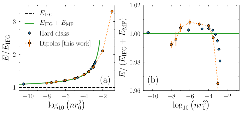
Figure 1: (a) Equation of state for the unpolarized system ($P=0$) in units of the ideal-Fermi-gas energy $E_{\mathrm{IFG}}$. DMC data for the dipolar gas (orange circles – orange dotted lines are a guide to the eye) are compared to the IFG and MF curves (black dashed line and green solid line) and to the DMC energy for hard disks (blue diamonds, from Ref. Bertaina (2013), with disk diameter $a_{s}=e^{2\gamma}r_{0}$). (b) Same as in panel (a), in units of the MF equation of state. In panel (a), statistical uncertainties on the DMC energies (orange circles) are smaller than the symbol size.

Also the case of a single-species bosonic gas of dipoles in two dimensions was studied through DMC, to compute the equation of state and compare it with a mean-field approximation Astrakharchik et al. (2009). High-precision energies were obtained for densities down to $nr_{0}^{2}=10^{-100}$, where the beyond-mean-field energy correction remains as large as 1%. An analogous precision, which is necessary to properly describe the subtle beyond-mean-field contribution, is beyond the scope of the current work.

Apart from the benchmark of approximate theories, it is instructive to compare the low-density equation of state for dipoles with the one for a different model of repulsive fermions, namely hard disks. In the case of bosons, a universal regime exists for densities below $nr_{0}^{2}\approx 10^{-7}$, where the energy of these two models only depends on the gas parameter $na_{s}^{2}$ Pilati et al. (2005); Astrakharchik et al. (2009). To establish such comparison in the fermionic case, we consider hard disks with diameter and scattering length both equal to the scattering length of dipoles, $a_{s}=r_{0}e^{2\gamma}$. The DMC equation of state for hard disks from Ref. Bertaina (2013) is in reasonable agreement with the one for dipoles [see Fig. 1(a)]. This behavior hints at the presence of a universal low-density regime, where the energy only depends on the gas parameter $na_{s}^{2}$. Nevertheless, we observe a small deviation between the energies of dipoles and hard disks, highlighted in Fig. 1(b). The residual difference suggests that the universal region would start at even lower density, when compared to the hard-disk case. This is because the dipolar potential, in spite of its formal short-ranged nature, has a slow power-law decay at large distance [see also the discussion about pair distribution functions in Section III.3]. The effect of higher partial waves may also contribute to the energy deviations.

Notice that backflow corrections are negligible for computing the equation of state at low density, as in Fig. 1. They become important at high density, especially when one needs to evaluate the small energy difference between the polarized and unpolarized states. This is the case for the study of itinerant ferromagnetism, where the bias stemming from the fixed-node prescription becomes crucial – see Section IV.

III.3 Pair distribution functions

As part of the characterization of the balanced mixture of fermionic dipoles, we compute the same-species and different-species pair distribution functions [$g_{\uparrow\uparrow}(r)$ and $g_{\uparrow\downarrow}(r)$, respectively] for both low and high densities – see Fig. 2. As a reference, we compare our results to the equivalent curves for the IFG: $g_{\uparrow\downarrow}(r)=1$ and $g_{\uparrow\uparrow}(r)=1-\left(2J_{1}(\tilde{r})/\tilde{r}\right)^{2}$, where $\tilde{r}\equiv(4\pi n_{\uparrow})^{1/2}r$ and $J_{1}$ is the Bessel function of the first kind Giuliani and Vignale (2005).

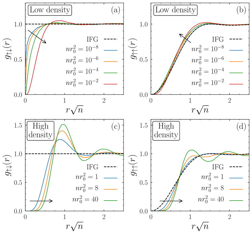
Figure 2: Pair distribution functions for the $P=0$ state, computed through DMC (solid lines), for different-species [panels (a) and (c)] and same-species pairs [panels (b) and (d)]. The analytic IFG distribution functions are also shown (dashed black lines). Arrows point towards increasing $nr_{0}^{2}$. The particle numbers are $N=74$ (for $nr_{0}^{2}<1$), $N=98$ (for $nr_{0}^{2}=1$) and $N=122$ (for $nr_{0}^{2}>1$). The trial wave functions are $\Psi_{\mathrm{JS}}$ for $nr_{0}^{2}<1$ and $\Psi_{\mathrm{BF}}$ for $nr_{0}^{2}\geq 1$. Statistical error bars are of the order of the line width.

At low density, $g_{\uparrow\downarrow}(r)$ is similar to the IFG curve, apart from a short-distance suppression due to dipolar repulsion – cf. Fig. 2(a). In the same density regime, $g_{\uparrow\uparrow}(r)$ displays a different behavior [see Fig. 2(b)]: At density $nr_{0}=10^{-8}$ it is indistinguishable from the corresponding IFG curve, and for increasing densities (up to $nr_{0}^{2}\lesssim 10^{-4}$) it shifts towards smaller values of $r\sqrt{n}$. The $g_{\uparrow\uparrow}(r)$ curve for $nr_{0}^{2}=10^{-2}$, in contrast, intersect with the ones for lower densities [cf. red line in Fig. 2(b)]. We interpret this change of behavior as the departure from the weakly-interacting regime.

At low-enough density $nr_{0}^{2}$ or at small-enough distance $r$, the probability of having three particles at distance $r$ from each other is suppressed, and $g_{\uparrow\downarrow}(r)$ only depends on two-body properties. The solution of the Schrödinger equation for two dipoles in vacuum is $\varphi(r)\propto K_{0}(2\sqrt{r_{0}/r})$, with $K_{0}$ the modified Bessel function Macia et al. (2011). Our DMC data confirm that the $g_{\uparrow\downarrow}(r)$ curves for different densities collapse onto $|\varphi(r)|^{2}$, at short distance, after the rescaling by a density-dependent constant prefactor $B$ – see Fig. 3. Deviations from this behavior appear at a distance which is proportional to $1/\sqrt{n}$, so that the two-body window becomes smaller for higher densities.

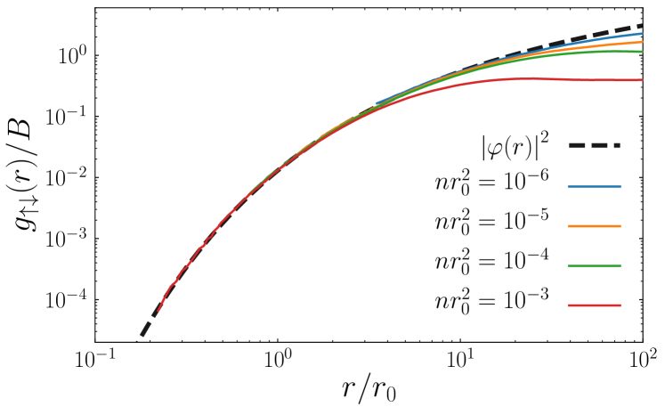
Figure 3: Pair distribution function $g_{\uparrow\downarrow}(r)$ at small distance, for different densities (solid lines from top to bottom are for densities from $nr_{0}^{2}=10^{-6}$ to $nr_{0}^{2}=10^{-3}$). Each curve is fitted to $B|\varphi(r)|^{2}$ in the small-$r$ regime, and plotted in units of $B$ to highlight the collapse onto the squared two-body wave function $|\varphi(r)|^{2}$ (black dashed line). Notice that the value of $B$ depends on the density $nr_{0}^{2}$. Statistical error bars are of the order of the line width.

Despite its slow decay at large distance, the $1/r^{3}$ interaction is formally short-ranged in two dimensions. The wave function $\varphi(r)$ for the two-body problem in vacuum scales as $\log r$ at large $r$, as for other short-range models. For such potentials there exists a universal window where $g_{\uparrow\downarrow}(r)\propto\log^{2}r$, for distances much larger than the potential range and much smaller than the typical interparticle distance. The constant prefactor of $\log^{2}r$ is Tan’s contact parameter, and a set of universal expressions connects it to other observables Werner and Castin (2012). This behavior is expected also for the dipolar gas, but the slow decay of $1/r^{3}$ is reflected in a slow convergence of $\varphi(r)$ towards its asymptotic form. The universal window is not present for the densities considered in this work, and would only appear for higher values of $1/\sqrt{n}$ (that is, for lower density). Thus it is not feasible to fit a $\log^{2}r$ curve to the data in Fig. 3, at odds with the case of short-range potentials like hard disks Bertaina (2013). This non-universality is consistent with the observed deviations of the equation of state for the dipolar gas from the one for hard disks (see Fig. 1). The universal regime would appear at even lower densities, which are unrealistic for current experiments.

Also in the high-density regime [$nr_{0}^{2}\geq 1$, see Fig. 2(c) and (d)], $g_{\uparrow\downarrow}(r)$ reflects the dipolar repulsion, showing the oscillatory behavior that corresponds to the formation of shells of neighbors around a specific particle. As the interaction strength increases, the height of the first peak becomes larger. Particles of the same species, on the contrary, are kept farther apart due to the Pauli exclusion principle. A direct consequence is that the first peak of $g_{\uparrow\uparrow}(r)$ is suppressed, as compared to the one in $g_{\uparrow\downarrow}(r)$. At $nr_{0}^{2}=1$ the first peak is invisible, at $nr_{0}^{2}=8$ it is visible but lower than the second one, and at $nr_{0}^{2}=40$ the two are comparable [see Fig. 2(d)].

The effect of using $\Psi_{\mathrm{BF}}$ rather than $\Psi_{\mathrm{JS}}$, when computing pair distribution functions within DMC, is negligible for densities $nr_{0}^{2}\ll 1$ (at the scale considered). For the other cases reported in Fig. 2, with $nr_{0}^{2}\geq 1$, we explicitly evaluated the backflow correction to $g_{\sigma_{1}\sigma_{2}}(r)$ through the comparison of results obtained by using $\Psi_{\mathrm{BF}}$ or $\Psi_{\mathrm{JS}}$. At the largest density ($nr_{0}^{2}=40$), the maximum absolute effect is a variation of $0.04$ close to the first peak, both for $g_{\uparrow\uparrow}(r)$ and $g_{\uparrow\downarrow}(r)$. This corresponds to less than a 6% relative change in the pair distribution functions.

IV Itinerant ferromagnetism

In Sections IV.1 and IV.2, we present two standard methods to look for a ferromagnetic instability, both based on commonly used trial wave functions ($\Psi_{\mathrm{JS}}$ and $\Psi_{\mathrm{BF}}$): The direct comparison of the energy for many-body states with $P=0$ and $P=1$, and the comparison of the polaron energy with the chemical potential of the fully-polarized gas. The inconclusive numerical results constitute a motivation for resorting to more accurate trial wave functions for DMC, as reported in Section IV.3.

IV.1 Direct energy comparison for $P=0$ and $P=1$

A direct method to look for a ferromagnetic instability is to compute the difference between the energy per particle of the unpolarized and polarized states,

$$\Delta E\equiv E_{P=0}-E_{P=1}.$$ (11)

The two states are simulated by using trial wave functions with different nodal structures. For $P=0$ the antisymmetric part of $\Psi_{T}$ is the product of two Slater determinants [one for each species, as in Eq. (5)], while a single one is needed for $P=1$.

We compute $\Delta E$ twice, with the SJ and BF trial wave functions. In both cases we find a critical density at which $\Delta E$ crosses zero and becomes positive, which signals a region where the system features a magnetic instability towards a polarized state – see Fig. 4. This crossing point only provides an upper bound for the onset of ferromagnetism, since in principle a partially-polarized state (with $0<P<1$) could be the ground state even at lower density.

The crossing between $P=0$ and $P=1$ takes place at density $nr_{0}^{2}$ approximately equal to 20 when using $\Psi_{\mathrm{JS}}$, and to 26 when using $\Psi_{\mathrm{BF}}$ – see Fig. 4 and Table 1. The shift of the crossing density is mainly due to the large backflow correction to the $P=0$ energy [see fourth and seventh columns in Table 1], as in the case of the three-dimensional electron gas Zong et al. (2002). It is known from previous calculations on liquid ³He that spherically-symmetric backflow correlations have a small effect in the polarized phase Pandharipande and Bethe (1973); Manousakis et al. (1983). For the dipolar gas, the relative energy difference between $P=1$ and $P=0$ is extremely small (below $5\cdot 10^{-4}$, for calculations with $\Psi_{\mathrm{BF}}$ at density $nr_{0}^{2}$ between $24$ and $48$). These two elements (the clear shift in the crossing density and the small energy differences) suggest that the fixed-node bias is crucial and may lead to qualitatively different results when using a different nodal structure, as we show in Section IV.3. This is especially important because the relevant density window for a hypothetical polarized phase has an upper bound at $nr_{0}^{2}\approx 50$, the freezing density for the $P=1$ state Matveeva and Giorgini (2012).

We stress that data in Table 1 and Fig. 4 are obtained for systems of finite size ($N=121,122$), chosen as large as possible to minimize the size dependence of both the kinetic and potential energies. A study of the scaling of $E$ with respect to $N$ reveals that the residual finite-size dependence of the energies does not modify the result about the existence of the $\Delta E=0$ energy crossing.

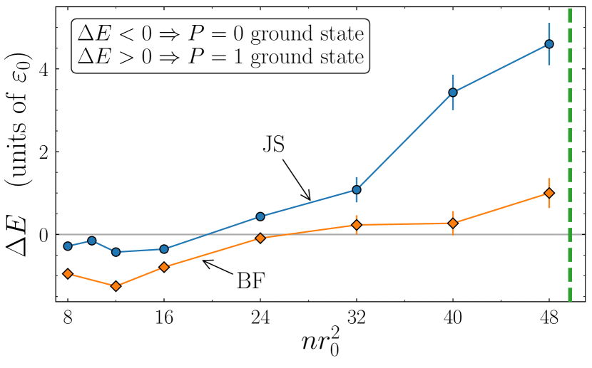
Figure 4: Difference in the energy per particle between $P=0$ and $P=1$ states [cf. Eq. (11)], computed through DMC with the Jastrow-Slater (JS) or Backflow (BF) trial wave function (see Table 1). Statistical error bars are shown, and lines are a guide to the eye. The vertical dashed line marks the freezing density for the $P=1$ state Matveeva and Giorgini (2012).

		$P=1$			$P=0$
$nr_{0}^{2}$	$E_{\mathrm{JS}}$	$E_{\mathrm{BF}}$	Corr.	$E_{\mathrm{JS}}$	$E_{\mathrm{BF}}$	Corr.
8	168.66(1)	168.63(1)	0.03(1)	168.38(2)	167.68(4)	0.70(4)
12	295.98(2)	295.92(2)	0.06(3)	295.55(6)	294.67(5)	0.88(8)
16	442.22(2)	442.04(2)	0.18(3)	441.87(7)	441.25(6)	0.6(1)
24	781.21(4)	780.8(1)	0.4(1)	781.6(1)	780.71(7)	0.9(1)
32	1172.45(5)	1171.9(1)	0.6(1)	1173.5(3)	1172.1(2)	1.4(4)
40	1608.0(1)	1607.7(1)	0.3(2)	1611.4(4)	1607.9(2)	3.5(5)
48	2083.1(1)	2083.0(2)	0.1(2)	2087.7(5)	2084.0(3)	3.7(6)
64	3137.7(1)	3137.4(2)	0.3(2)	3145.4(8)	3139.8(3)	5.6(9)

Table 1: DMC energy per particle (in units of $\varepsilon_{0}$) at different densities. Data for $P=1$ ($P=0$) are obtained with $N=121$ ($N=122$) particles. Columns marked as “Corr.” indicate the energy correction $E_{\mathrm{JS}}-E_{\mathrm{BF}}$. Statistical errors are reported in parentheses.

IV.2 Stability of $P=1$ state

An alternative approach to look for itinerant ferromagnetism consists in computing the energy cost or gain for a spin-flip excitation on top of a fully polarized state. If the $P=1$ state is the ground state, then any excitation must lead to a state with higher energy. If the true ground state has polarization $P<1$, on the contrary, a single spin flip on top of a fully-polarized state may decrease its energy, signalling the instability of the $P=1$ state.

Through the DMC technique, we have access to the energy per particle $E_{(N_{\uparrow},N_{\downarrow})}$, for any choice of $(N_{\uparrow},N_{\downarrow})$. For a given $N_{\uparrow}$, the polaron energy $\varepsilon_{p}$ and the $P=1$ chemical potential $\mu$ read

$$\varepsilon_{p}^{(N_{\uparrow})} \equiv(N_{\uparrow}+1)E_{(N_{\uparrow},1)}-N_{\uparrow}E_{(N_{\uparrow},0)},$$ (12)

$$\mu^{(N_{\uparrow})} \equiv(N_{\uparrow}+1)E_{(N_{\uparrow}+1,0)}-N_{\uparrow}E_{(N_{\uparrow},0)},$$ (13)

where both quantities are defined at fixed surface $L^{2}$ (notice that this leads to a density difference between systems of $N_{\uparrow}$ and $N_{\uparrow}+1$ particles, which vanishes as $1/N_{\uparrow}$ in the thermodynamic limit).

In a large system, a single spin flip on top of a fully-polarized state induces a change in the total energy which is

$$\Delta E_{\mathrm{flip}}=\varepsilon_{p}^{(\infty)}-\mu^{(\infty)}.$$ (14)

If $\Delta E_{\mathrm{flip}}>0$, then the $P=1$ state is robust against a single spin-flip excitation and might be the true ground state, while for a negative $\Delta E_{\mathrm{flip}}$ such state is unstable.

To be in the region where the ground state may have polarization $P=1$, we consider the density $n_{\uparrow}r_{0}^{2}=40$ (cf. Fig. 4, and notice that $n=n_{\uparrow}$ in the thermodynamic limit), where we perform calculations with the $\Psi_{\mathrm{JS}}$ trial wave function. The polaron energy has a strong dependence on the system size, so that a finite-size-scaling study is necessary. We find that DMC results are in reasonable agreement with a linear scaling, $\varepsilon_{p}^{(N_{\uparrow})}=\varepsilon_{p}^{(\infty)}+\beta/N_{\uparrow}$ (see Fig. 5). The best-fit result is $\varepsilon_{p}^{(\infty)}/(\hbar^{2}n_{\uparrow}/m)=97.7(3)$.

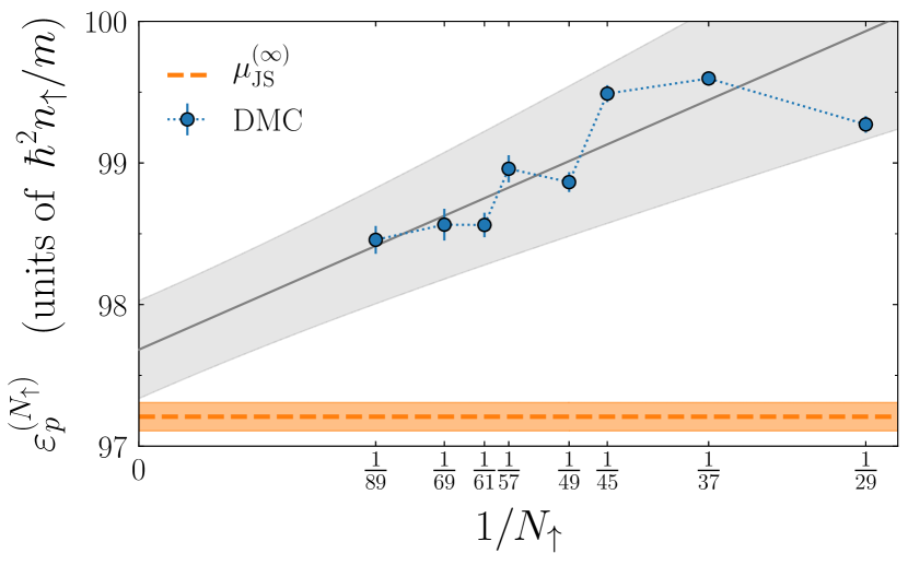
Figure 5: Size scaling of the DMC polaron energy at density $n_{\uparrow}r_{0}^{2}=40$, in units of $\hbar^{2}n_{\uparrow}/m$ (blue circles – blue dotted line is a guide to the eye). For the linear fit (gray solid line), the shaded band includes both the statistical uncertainty and the systematic error due to the choice of the fit range. The $P=1$ chemical potential $\mu_{\mathrm{JS}}^{(\infty)}$ (orange horizontal dashed line, with shaded area representing its uncertainty) is extracted from the equation of state – see text. All calculations are based on the $\Psi_{\mathrm{JS}}$ trial wave function.

The chemical potential can be computed directly from the equation of state, as

$$\mu^{(N_{\uparrow})}=\left(1+n_{\uparrow}\frac{\partial}{\partial n_{\uparrow}}\right)E_{(N_{\uparrow},0)}.$$ (15)

We apply this definition to the JS equation of state of a large system (cf. Table 1). We fit the energy per particle with the expression $A_{1/2}n_{\uparrow}^{1/2}+A_{1}n_{\uparrow}+A_{5/4}n_{\uparrow}^{5/4}+A_{3/2}n_{\uparrow}^{3/2}$ Astrakharchik et al. (2007a), from which we obtain $\mu_{\mathrm{JS}}^{(\infty)}/(\hbar^{2}n_{\uparrow}/m)=97.2(1)$, for $n_{\uparrow}r_{0}^{2}=40$. The error bar includes the statistical uncertainty and a systematic error due to finite-size effects.

The result concerning the stability against a spin flip, namely the sign of $\Delta E_{\mathrm{flip}}$, is affected by strong statistical and systematic uncertainties. Since the polaron energy has a sizable dependence on $N_{\uparrow}$ (see Fig. 5), convergence would only be obtained for larger system sizes. Such calculations are hindered by the fact that $\varepsilon_{p}^{(N_{\uparrow})}$ is computed as the difference between two extensive observables, which makes it challenging to reach large system sizes while keeping the statistical uncertainties under control. An alternative method consists in estimating the difference between the total energy of two systems with the same number of particles and density, namely with $(N_{\uparrow},N_{\downarrow})$ equal to $(N-1,1)$ and $(N,0)$. This approach reduces the size dependence of $\varepsilon_{p}^{(N_{\uparrow})}$, and in the case of a bosonic bath it was successfully combined with the correlated-sampling technique Boronat and Casulleras (1999). For fermions, however, it introduces an additional correction due to the change in the nodal structure of the $\uparrow$ component, and we found that it reaches a precision similar to the one reported in this work.

In conclusion, we find that $\Delta E_{\mathrm{flip}}>0$ at density $nr_{0}^{2}=40$, pointing towards the stability of the $P=1$ state. However, the large uncertainties on $\Delta E_{\mathrm{flip}}$ make this result inconclusive, and we cannot use it as a reliable confirmation of the fully-polarized ground state identified in Section IV.1 for densities higher than $nr_{0}^{2}\approx 26$.

IV.3 Iterative-backflow wave functions

As observed above, the fixed-node bias cannot be neglected in the study of itinerant ferromagnetism. In this section we investigate this issue in detail, by making use of improved trial wave functions based on the iterative backflow transformations Taddei et al. (2015).

		$P=1$			$P=0$		$\Delta E_{T}$	$\Delta E$
$\Psi_{T}$	$\sigma_{T}^{2}$	$E_{T}$	$E$	$\sigma_{T}^{2}$	$E_{T}$	$E$
JS	102(8)	1615.98(5)	1607.92(1)	311(10)	1636.56(8)	1610.85(5)	20.6(1)	2.93(6)
JS3	47(2)	1610.90(3)	-	185(6)	1625.21(6)	-	14.31(6)	-
BF	40(2)	1609.28(3)	1607.09(2)	98(2)	1613.94(17)	1606.91(17)	4.7(2)	-0.2(2)
BF3	28.5(8)	1608.59(7)	1606.94(4)	96(2)	1612.63(7)	1606.29(6)	4.0(1)	-0.65(7)
IT1	32.6(7)	1608.40(7)	1606.91(3)	78(1)	1610.78(11)	1605.69(9)	2.38(13)	-1.22(1)
BF3-IT1	26.8(5)	1608.15(7)	1606.87(5)	75(2)	1609.65(11)	1605.57(6)	1.50(13)	-1.31(8)
IT2	30.6(7)	1608.02(6)	1606.91(6)	74.8(9)	1609.54(7)	1605.31(13)	1.52(9)	-1.59(14)
VMCext		1605.3(5)			1602(1)

Table 2: Variance and energy per particle at density $nr_{0}^{2}=40$, in units of $\varepsilon_{0}$, for different trial wave functions $\Psi_{T}$. The variational energy per particle $E_{T}$ and the DMC result $E$ are reported, and for $E_{T}$ we also report the variance $\sigma_{T}^{2}$. The last two columns report the energy difference between the unpolarized and polarized states, for variational results [$\Delta E_{T}\equiv E_{T,P=0}-E_{T,P=1}$] and for DMC energies [$\Delta E$, cf. Eq. (11)]. The line “VMC_ext” is obtained through a linear extrapolation of the $E_{T}$ values – see text. Data for $P=1$ ($P=0$) are obtained with $N=121$ ($N=122$) particles. For the details about the wave functions, and for a comparison with Table 1, see Appendix A. Note that the JS and JS3 wave functions have the same nodal structure, so that their DMC energies should be the same within statistical uncertainty.

Given a variational ansatz $\Psi_{T}$, the energy per particle $E_{T}$ and its variance $\sigma_{T}^{2}$ are defined as

$$E_{T} \equiv\frac{\left\langle\Psi_{T}\right|H\left|\Psi_{T}\right\rangle}{N},$$ (16)

$$\sigma^{2}_{T} \equiv\frac{\left\langle\Psi_{T}\right|\left(H-NE_{T}\right)^{2}\left|\Psi_{T}\right\rangle}{N^{2}}.$$ (17)

These two observables are related to the quality of the ansatz Mora and Waintal (2007): When $\Psi_{T}$ approaches an eigenstate $\Psi_{0}$ of $H$, $E_{T}$ tends to $E_{0}\equiv\langle\Psi_{0}|H|\Psi_{0}\rangle/N$ and $\sigma^{2}_{T}$ tends to zero. Rigorous bounds connect $E_{T}$ to $E_{0}$ and $\sigma_{T}^{2}$ Temple and Chapman (1928); Weinstein (1934); Goedecker and Maschke (1991). We assume that the eigenstate $\Psi_{0}$ closest in energy to $\Psi_{T}$ is the ground state, so that $E_{0}$ is the ground-state energy per particle. We also assume that $\langle\Psi_{T}|\Psi_{0}\rangle$ is the only significant overlap of $\Psi_{T}$ with an eigenstate of $H$, which is reasonable for an extended system. In this case, we obtain a linear relation between $\sigma_{T}^{2}$ and $E_{T}$ Taddei et al. (2015),

$$E_{T}=E_{0}+NA\sigma_{T}^{2}\qquad\text{for $\sigma_{T}^{2}\to 0$},$$ (18)

where $A$ is a constant coefficient.

Eq. (18) provides a practical way to estimate the true ground-state energy $E_{0}$, by computing $\sigma^{2}_{T}$ and $E_{T}$ for several trial wave functions (through the Variational Monte Carlo method) and performing a linear extrapolation towards $\sigma_{T}^{2}=0$. The validity of this extrapolation was verified for both ³He and ⁴He Taddei et al. (2015); Ruggeri et al. (2018). For ³He, the technique can be benchmarked against independent calculations of the ground-state energy, obtained through the transient-estimate method for polarized and unpolarized systems. The result is that the energy-variance extrapolated energy has an accuracy comparable with the best available DMC results Taddei et al. (2015).

We applied this extrapolation scheme to the variational energies of the polarized and unpolarized dipolar Fermi gas at density $nr_{0}^{2}=40$, as shown in Fig. 6. For any choice of $\Psi_{T}$, the energy difference $\Delta E_{T}\equiv E_{T,P=0}-E_{T,P=1}$ is positive (see 8th column in Table 2), indicating that the $P=1$ state is always favored at the variational level, for the wave functions considered here. Nevertheless, the energy gain in using a better trial wave function is more relevant for the $P=0$ state (cf. $E_{T}$ columns in Table 2), as noted in Section IV.1. As a consequence, the energy difference $\Delta E_{T}$ decreases upon improving the trial wave function. We fit the data for $E_{T}$ with Eq. (18), finding a reasonable linear scaling. We then estimate the true ground-state energy through the intercept with the vertical axis, and we find that the lowest energy corresponds to the $P=0$ state. We conclude that the fully-polarized state is not the ground state at density $nr_{0}^{2}=40$.

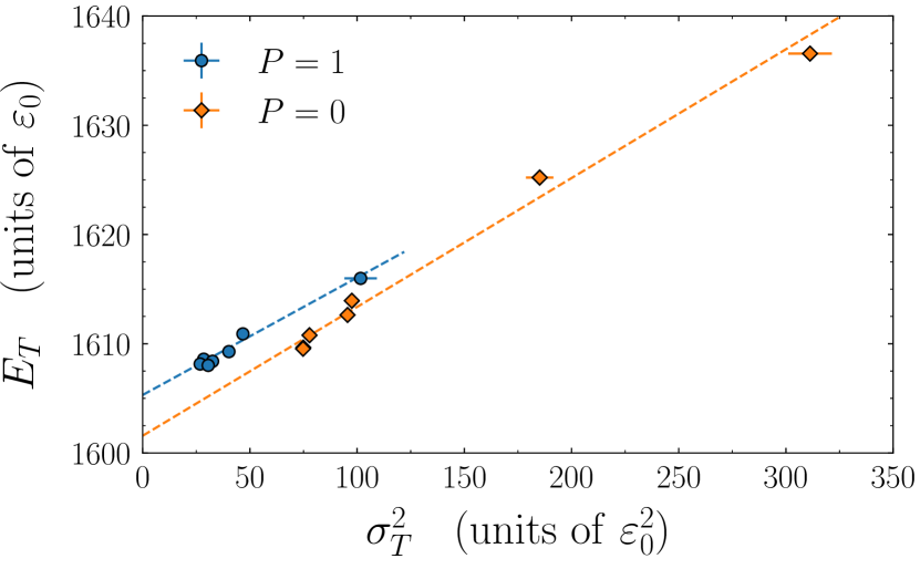
Figure 6: Scaling of the energy per particle vs its variance, for different variational wave functions, at polarizations $P=1$ (blue circles) and $P=0$ (orange diamonds) – cf. Table 2. Dashed lines are linear fits to the data, see Eq. (18).

An independent confirmation comes from the fixed-node DMC energies for simulations based on the iterative-backflow wave functions – see Table 2. For $P=1$, our four best choices for the nodal structure yield energies which are compatible with each other within statistical uncertainties. For $P=0$, the energy dependence on the wave function is larger, and the lowest energy is reached through the iterative-backflow wave function IT2. As reported in the last column of Table 2, and at a difference with the case of variational energies, the DMC energy difference $\Delta E$ becomes negative when the accuracy of the nodal structure increases. The best available DMC energies are indeed lower for the $P=0$ state, in agreement with the energy-variance extrapolation.

The evidence for the fact that the ground state is not fully polarized extends to the density $nr_{0}^{2}=48$ Comparin et al. (2018). In that case, the best DMC energy for $P=1$, $E_{\mathrm{BF3-IT1}}=2081.69(5)$, is still higher than the one for $P=0$, $E_{\mathrm{BF3-IT1}}=2080.49(15)$. Also the energy-variance extrapolation leads to the same conclusion. Therefore, we exclude the existence of a fully-polarized ground state for densities up to $nr_{0}^{2}=48$.

V Discussion and conclusions

We performed the first study of the $P=0$ mixture of dipolar fermions, both at low and high density, computing the equation of state and pair distribution functions through the DMC technique. For density below $nr_{0}^{2}\approx 10^{-3}$, the equation of state agrees within a few percent both with a mean-field approximation and with the energy of fermionic hard disks. Non-universal beyond-mean-field corrections are present for higher densities.

Two assumptions of the theoretical model need to be discussed, in view of a connection to experiments with ultracold atoms or molecules: The reduced dimensionality and the shape of the interparticle potential. The experimental realization of a two-dimensional system is based on a tight confinement along the transverse direction, characterized by the harmonic-oscillator length $a_{z}$ or by the typical energy $\hbar\omega_{z}$. At zero temperature, the condition to be in the two-dimensional regime reads $\mu\ll\hbar\omega_{z}$, where $\mu$ is the chemical potential, which is of the order of $E_{\mathrm{IFG}}$. Such condition corresponds to $nr_{0}^{2}\ll({r_{0}}/{a_{z}})^{2}$, showing that the maximum allowed value of $nr_{0}^{2}$ depends on the ratio $a_{z}/r_{0}$. By setting $r_{0}\approx 20$ nm (the value for Dy atoms) and choosing a realistic value $a_{z}\approx 500$ nm, we find that the confined system can be described by a two-dimensional model up to $nr_{0}^{2}\approx 10^{-3}$. This density is comparable with the one where beyond-mean-field corrections to the equation of state become important.

The second issue is that our model neglects the presence of an additional contact interaction, on top of the dipolar repulsion. On the one hand, the two-dimensional scattering length for a three-dimensional contact interaction with scattering length $a_{3D}$ scales as $\exp(-\sqrt{\frac{\pi}{2}}a_{z}/a_{3D})$, in presence of transverse confinement Pitaevskii and Stringari (2016). Thus it is strongly suppressed when $a_{3D}\ll a_{z}$, which is the typical case away from Feshbach resonances. On the other hand, the two-dimensional scattering length of the dipolar potential is of the order of $r_{0}$, independently on $a_{z}$. For this reason, the lack of a contact interaction in our model should not have a relevant effect on the equation of state, at the experimentally realistic densities $nr_{0}^{2}=10^{-3}-10^{-1}$.

When moving towards high values of $nr_{0}^{2}$, the aforementioned condition for being in the two-dimensional regime implies that a large value of $r_{0}/a_{z}$ is needed. This is currently beyond reach for the permanent magnetic moment of atoms, but could be achieved for a gas of molecules with a large induced dipole moment – see for instance Refs. Ni et al. (2010); Park et al. (2015).

At high density, we find that the issue of itinerant ferromagnetism is extremely subtle due to the small energy differences at play. Thus it requires a high degree of accuracy in the nodal structure, to be treated within the fixed-node scheme. In our analysis we observe no signature of a fully-polarized ground state, up to a density approximately equal to the freezing density. Once the freezing transition is crossed, we expect a weak dependence of the energy on the polarization, in analogy with the case of the two-dimensional electron gas Drummond and Needs (2009). In principle there may exist an intermediate-density regime where the ground state is partially polarized, with $0<P<1$, as in the case of three-dimensional hard-core fermions Pilati et al. (2010). This possibility remains open, as our current study of dipolar fermions is restricted to polarization $P=0$ and $1$.

We also demonstrate the usefulness of iterative-backflow wave functions in a novel system, where the accuracy of the common JS/BF wave functions is inadequate for the study of itinerant ferromagnetism. The combination of high-accuracy DMC results with the energy-variance extrapolation of variational data provides a clear indication about the energies of the polarized and unpolarized states, and meanwhile constitutes an estimate of the fixed-node bias for the two cases.

Appendix A Trial wave functions for Section  IV.3

In this appendix, we describe the trial wave functions used in Section IV.3. The corresponding numerical results are obtained through an independent implementation of the DMC algorithm, with respect to the rest of the manuscript.

The JS and JS3 wave functions are of the standard Jastrow-Slater form, with two-body (JS) or two- and three-body (JS3) Jastrow correlations Holzmann et al. (2006). Each Jastrow correlation function is parametrized via locally piecewise–quintic Hermite interpolants (splines) with typically 38 variational parameters per function Natoli and Ceperley (1995); Holzmann and Bernu (2005). Although the variational energies $E_{T}$ of the JS and JS3 wave function are different (see Table 2), the two DMC energies have to be the same since the two wave functions share the same nodal structure. Moreover, the JS results of our two independent implementations of the DMC algorithm agree within error bars (compare Table 1 with Table 2, for density $nr_{0}^{2}=40$), which constitutes an additional validity check.

The BF wave function includes two-body backflow correlations as in Eq. (6), with $f_{\mathrm{BF}}(r)$ parametrized through Hermite interpolants (as in the case of Jastrow correlations). Different choices of $f_{\mathrm{BF}}(r)$ correspond to different nodal structures, so that also the DMC energy can differ. As an example, the DMC energy for the BF wave function parametrized as in Ref. Grau et al. (2002) is larger than the one where $f_{\mathrm{BF}}(r)$ is parametrized through splines – cf. “BF” entries in Table 1 (for $nr_{0}^{2}=40$) and in Table 2. Note that this does not affect the conclusions of this work. In the BF3 case, also an explicit three-body backflow correction is included, as in Ref. Holzmann et al. (2006).

As a starting point of the iterative backflow procedure, we choose the IT0 wave function (that is, the one with $\alpha=0$) to be the Jastrow-Slater wave function with two-body Jastrow correlations. At each iteration $\alpha\to\alpha+1$, we perform an additional transformation from $\mathbf{q}_{i}^{(\alpha)}$ to

$$\mathbf{q}_{i}^{(\alpha+1)}\equiv\mathbf{q}_{i}^{(\alpha)}+\sum_{j\neq i}\left(\mathbf{q}_{i}^{(\alpha)}-\mathbf{q}_{j}^{(\alpha)}\right)f_{\mathrm{BF}}^{(\alpha)}\left(|\mathbf{q}_{i}^{(\alpha)}-\mathbf{q}_{j}^{(\alpha)}|\right),$$ (19)

where $\mathbf{q}_{i}^{(0)}=\mathbf{x}_{i}$ are the particle coordinates. This procedure leads to the IT1 and IT2 wave functions. The iterative-backflow transformations $f_{\mathrm{BF}}^{(\alpha)}(r)$ are parametrized via three-parameters Gaussian functions, $A\exp\left[-B(r-C)^{2}\right]$, additionally imposing that the function and its derivative vanish at $r=L/2$. The “bare” Jastrow and backflow potentials are still treated via Hermite interpolants.

For the BF3IT1 wave function we combine the non-iterated three-body backflow correlation (as in the BF3 wave function) with an iterated two-body backflow and Jastrow potential (as in the IT1 wave function).

References

- Dalfovo et al. (1999) F. Dalfovo, S. Giorgini, L. P. Pitaevskii, and S. Stringari, Rev. Mod. Phys. 71, 463 (1999).
- Giorgini et al. (2008) S. Giorgini, L. P. Pitaevskii, and S. Stringari, Rev. Mod. Phys. 80, 1215 (2008).
- Baranov (2008) M. A. Baranov, Phys. Rep. 464, 71 (2008).
- Lahaye et al. (2009) T. Lahaye, C. Menotti, L. Santos, M. Lewenstein, and T. Pfau, Rep. Progr. Phys. 72, 126401 (2009).
- Bohn et al. (2017) J. L. Bohn, A. M. Rey, and J. Ye, Science 357, 1002 (2017).
- Santos et al. (2000) L. Santos, G. V. Shlyapnikov, P. Zoller, and M. Lewenstein, Phys. Rev. Lett. 85, 1791 (2000).
- Aikawa et al. (2014) K. Aikawa, S. Baier, A. Frisch, M. Mark, C. Ravensbergen, and F. Ferlaino, Science 345, 1484 (2014).
- Baier et al. (2016) S. Baier, M. J. Mark, D. Petter, K. Aikawa, L. Chomaz, Z. Cai, M. Baranov, P. Zoller, and F. Ferlaino, Science 352, 201 (2016).
- Chomaz et al. (2016) L. Chomaz, S. Baier, D. Petter, M. J. Mark, F. Wächtler, L. Santos, and F. Ferlaino, Phys. Rev. X 6, 041039 (2016).
- Ferrier-Barbut et al. (2016) I. Ferrier-Barbut, H. Kadau, M. Schmitt, M. Wenzel, and T. Pfau, Phys. Rev. Lett. 116, 215301 (2016).
- Schmitt et al. (2016) M. Schmitt, M. Wenzel, F. Böttcher, I. Ferrier-Barbut, and T. Pfau, Nature 539, 259 (2016).
- Baier et al. (2018) S. Baier, D. Petter, J. H. Becher, A. Patscheider, G. Natale, L. Chomaz, M. J. Mark, and F. Ferlaino, Phys. Rev. Lett. 121, 093602 (2018).
- Trautmann et al. (2018) A. Trautmann, P. Ilzhöfer, G. Durastante, C. Politi, M. Sohmen, M. J. Mark, and F. Ferlaino, Phys. Rev. Lett. 121, 213601 (2018).
- Partridge et al. (2006) G. B. Partridge, W. Li, R. I. Kamar, Y.-a. Liao, and R. G. Hulet, Science 311, 503 (2006).
- Stamper-Kurn and Ueda (2013) D. M. Stamper-Kurn and M. Ueda, Rev. Mod. Phys. 85, 1191 (2013).
- Ni et al. (2010) K.-K. Ni, S. Ospelkaus, D. Wang, G. Quéméner, B. Neyenhuis, M. H. G. de Miranda, J. L. Bohn, J. Ye, and D. S. Jin, Nature 464, 1324 (2010).
- de Miranda et al. (2011) M. H. G. de Miranda, A. Chotia, B. Neyenhuis, W. D., G. Quéméner, S. Ospelkaus, J. L. Bohn, J. Ye, and D. S. Jin, Nat. Phys. 7, 502 (2011).
- Macia et al. (2014) A. Macia, G. E. Astrakharchik, F. Mazzanti, S. Giorgini, and J. Boronat, Phys. Rev. A 90, 043623 (2014).
- Bombin et al. (2017) R. Bombin, J. Boronat, and F. Mazzanti, Phys. Rev. Lett. 119, 250402 (2017).
- Bruun and Taylor (2008) G. M. Bruun and E. Taylor, Phys. Rev. Lett. 101, 245301 (2008).
- Cooper and Shlyapnikov (2009) N. R. Cooper and G. V. Shlyapnikov, Phys. Rev. Lett. 103, 155302 (2009).
- Büchler et al. (2007) H. P. Büchler, E. Demler, M. Lukin, A. Micheli, N. Prokof’ev, G. Pupillo, and P. Zoller, Phys. Rev. Lett. 98, 060404 (2007).
- Astrakharchik et al. (2007a) G. E. Astrakharchik, J. Boronat, I. L. Kurbakov, and Y. E. Lozovik, Phys. Rev. Lett. 98, 060405 (2007a).
- Matveeva and Giorgini (2012) N. Matveeva and S. Giorgini, Phys. Rev. Lett. 109, 200401 (2012).
- Hammond et al. (1994) B. L. Hammond, W. A. Lester, and P. J. Reynolds, Monte Carlo Methods in Ab Initio Quantum Chemistry (World Scientific, 1994).
- Foulkes et al. (2001) W. M. C. Foulkes, L. Mitas, R. J. Needs, and G. Rajagopal, Rev. Mod. Phys. 73, 33 (2001).
- Kolorenč and Mitas (2011) J. Kolorenč and L. Mitas, Rep. Progr. Phys. 74, 026502 (2011).
- Bloch (1929) F. Bloch, Z. Phys. 57, 545 (1929).
- Ceperley (1978) D. Ceperley, Phys. Rev. B 18, 3126 (1978).
- Ceperley and Alder (1980) D. M. Ceperley and B. J. Alder, Phys. Rev. Lett. 45, 566 (1980).
- Alder et al. (1982) B. J. Alder, D. M. Ceperley, and E. L. Pollock, Int. J. Quantum Chem. 22, 49 (1982).
- Tanatar and Ceperley (1989) B. Tanatar and D. M. Ceperley, Phys. Rev. B 39, 5005 (1989).
- Ortiz et al. (1999) G. Ortiz, M. Harris, and P. Ballone, Phys. Rev. Lett. 82, 5317 (1999).
- Zong et al. (2002) F. H. Zong, C. Lin, and D. M. Ceperley, Phys. Rev. E 66, 036703 (2002).
- Drummond and Needs (2009) N. D. Drummond and R. J. Needs, Phys. Rev. Lett. 102, 126402 (2009).
- Manousakis et al. (1983) E. Manousakis, S. Fantoni, V. R. Pandharipande, and Q. N. Usmani, Phys. Rev. B 28, 3770 (1983).
- Zong et al. (2003) F. H. Zong, D. M. Ceperley, S. Moroni, and S. Fantoni, Mol. Phys. 101, 1705 (2003).
- Nava et al. (2012) M. Nava, A. Motta, D. E. Galli, E. Vitali, and S. Moroni, Phys. Rev. B 85, 184401 (2012).
- Pilati et al. (2010) S. Pilati, G. Bertaina, S. Giorgini, and M. Troyer, Phys. Rev. Lett. 105, 030405 (2010).
- Chang et al. (2011) S.-Y. Chang, M. Randeria, and N. Trivedi, Proc. Nat. Acad. Sci. 108, 51 (2011).
- Arias de Saavedra et al. (2012) F. Arias de Saavedra, F. Mazzanti, J. Boronat, and A. Polls, Phys. Rev. A 85, 033615 (2012).
- Pilati et al. (2014) S. Pilati, I. Zintchenko, and M. Troyer, Phys. Rev. Lett. 112, 015301 (2014).
- He et al. (2016) L. He, X.-J. Liu, X.-G. Huang, and H. Hu, Phys. Rev. A 93, 063629 (2016).
- Vermeyen et al. (2018) E. Vermeyen, C. A. R. Sá de Melo, and J. Tempere, Phys. Rev. A 98, 023635 (2018).
- Zintchenko et al. (2016) I. Zintchenko, L. Wang, and M. Troyer, Eur. Phys. J. B 89, 180 (2016).
- Stoner (1938) E. C. Stoner, Proc. R. Soc. London, Ser. A 165, 372 (1938).
- Valtolina et al. (2017) G. Valtolina, F. Scazza, A. Amico, A. Burchianti, A. Recati, T. Enss, M. Inguscio, M. Zaccanti, and G. Roati, Nat. Phys. 13, 704 (2017).
- Jo et al. (2009) G.-B. Jo, Y.-R. Lee, J.-H. Choi, C. A. Christensen, T. H. Kim, J. H. Thywissen, D. E. Pritchard, and W. Ketterle, Science 325, 1521 (2009).
- Pekker et al. (2011) D. Pekker, M. Babadi, R. Sensarma, N. Zinner, L. Pollet, M. W. Zwierlein, and E. Demler, Phys. Rev. Lett. 106, 050402 (2011).
- Sanner et al. (2012) C. Sanner, E. J. Su, W. Huang, A. Keshet, J. Gillen, and W. Ketterle, Phys. Rev. Lett. 108, 240404 (2012).
- Amico et al. (2018) A. Amico, F. Scazza, G. Valtolina, P. E. S. Tavares, W. Ketterle, M. Inguscio, G. Roati, and M. Zaccanti, Phys. Rev. Lett. 121, 253602 (2018).
- Taddei et al. (2015) M. Taddei, M. Ruggeri, S. Moroni, and M. Holzmann, Phys. Rev. B 91, 115106 (2015).
- Ruggeri et al. (2018) M. Ruggeri, S. Moroni, and M. Holzmann, Phys. Rev. Lett. 120, 205302 (2018).
- Pitaevskii and Stringari (2016) L. Pitaevskii and S. Stringari, Bose-Einstein Condensation and Superfluidity (Oxford University Press, 2016).
- Drummond et al. (2011) N. D. Drummond, N. R. Cooper, R. J. Needs, and G. V. Shlyapnikov, Phys. Rev. B 83, 195429 (2011).
- Lin et al. (2001) C. Lin, F. H. Zong, and D. M. Ceperley, Phys. Rev. E 64, 016702 (2001).
- Anderson (1995) J. B. Anderson, Int. Rev. Phys. Chem. 14, 85 (1995).
- Macia et al. (2011) A. Macia, F. Mazzanti, J. Boronat, and R. E. Zillich, Phys. Rev. A 84, 033625 (2011).
- Grau et al. (2002) V. Grau, J. Boronat, and J. Casulleras, Phys. Rev. Lett. 89, 045301 (2002).
- Casulleras and Boronat (2000) J. Casulleras and J. Boronat, Phys. Rev. Lett. 84, 3121 (2000).
- Holzmann et al. (2006) M. Holzmann, B. Bernu, and D. M. Ceperley, Phys. Rev. B 74, 104510 (2006).
- Casulleras and Boronat (1995) J. Casulleras and J. Boronat, Phys. Rev. B 52, 3654 (1995).
- Lu and Shlyapnikov (2012) Z.-K. Lu and G. V. Shlyapnikov, Phys. Rev. A 85, 023614 (2012).
- Lange et al. (2016) P. Lange, J. Krieg, and P. Kopietz, Phys. Rev. A 93, 033609 (2016).
- Ticknor (2009) C. Ticknor, Phys. Rev. A 80, 052702 (2009).
- Schick (1971) M. Schick, Phys. Rev. A 3, 1067 (1971).
- Astrakharchik et al. (2009) G. E. Astrakharchik, J. Boronat, J. Casulleras, I. L. Kurbakov, and Y. E. Lozovik, Phys. Rev. A 79, 051602 (2009).
- Bertaina (2013) G. Bertaina, Eur. Phys. J. Spec. Top. 217, 153 (2013).
- Pilati et al. (2005) S. Pilati, J. Boronat, J. Casulleras, and S. Giorgini, Phys. Rev. A 71, 023605 (2005).
- Astrakharchik et al. (2007b) G. E. Astrakharchik, J. Boronat, J. Casulleras, I. L. Kurbakov, and Y. E. Lozovik, Phys. Rev. A 75, 063630 (2007b).
- Giuliani and Vignale (2005) G. Giuliani and G. Vignale, Quantum Theory of the Electron Liquid (Cambridge University Press, 2005).
- Werner and Castin (2012) F. Werner and Y. Castin, Phys. Rev. A 86, 013626 (2012).
- Pandharipande and Bethe (1973) V. R. Pandharipande and H. A. Bethe, Phys. Rev. C 7, 1312 (1973).
- Boronat and Casulleras (1999) J. Boronat and J. Casulleras, Phys. Rev. B 59, 8844 (1999).
- Mora and Waintal (2007) C. Mora and X. Waintal, Phys. Rev. Lett. 99, 030403 (2007).
- Temple and Chapman (1928) G. Temple and S. Chapman, Proc. R. Soc. London, Ser. A 119, 276 (1928).
- Weinstein (1934) D. H. Weinstein, Proc. Nat. Acad. Sci. 20, 529 (1934).
- Goedecker and Maschke (1991) S. Goedecker and K. Maschke, Phys. Rev. B 44, 10365 (1991).
- Comparin et al. (2018) T. Comparin, R. Bombin, M. Holzmann, F. Mazzanti, J. Boronat, and S. Giorgini, “Data 2D Fermi dipoles,” (2018), Zenodo.
- Park et al. (2015) J. W. Park, S. A. Will, and M. W. Zwierlein, Phys. Rev. Lett. 114, 205302 (2015).
- Natoli and Ceperley (1995) V. Natoli and D. M. Ceperley, J. Comput. Phys. 117, 171 (1995).
- Holzmann and Bernu (2005) M. Holzmann and B. Bernu, J. Comput. Phys. 206, 111 (2005).