Electric dipole spin resonance at shallow donors in quantum wires

Abstract

Electric dipole spin resonance is studied theoretically for a shallow donor formed in a nanowire with spin-orbit coupling in a magnetic field. Such system may represent a donor-based qubit. The single discrete energy level of the donor is accompanied by the set of continuum states, which provide a non-trivial interplay for the picture of electric dipole spin resonance driven by an external monochromatic field. Nonlinear dependencies of spin flip time as well as of the coordinate mean values on the electric field amplitude are observed, demonstrating the significance of coupling to the continuum for spin-based qubits manipulation in nanostructures.

I Introduction

Electric dipole spin resonance (EDSR), that is the ability to manipulate spins of charge carriers by electic rather than by a magnetic field, is one of the most distinctive features of spin-orbit coupling (SOC). Being theoretically predicted Rashba1960 and initially experimentally observed for itinerant electrons in bulk crystals Bemski1960 ; Bell1962 ; Bratashevskii1963 , soon it was studied theoretically in detail for electrons localized on donors Rashba1964a and for holes on the acceptor centers Rashba1964b . More recently, it was shown that the EDSR is a powerful tool for spin manipulation in quantum wells Rashba2003 and other two-dimensional heterostructures with spin-orbit coupling Azpiroz . In addition, the EDSR can be used to manipulate electic current in low-dimensional conductors Sadreev . Observation of the EDSR in quantum dots Nowack2007 opened a venue for their applications in spin-based quantum computing, where spin of a carrier localized in a quantum dot is considered as a qubit. Single electron spin manipulation using hybrid semiconductor-superconductor systems has been proposed in Ref. [Hu2012, ]. As result, theoretical studies of the EDSR in quantum dots became the field attracting a great interest of researchers Golovach2006 ; Jiang2006 ; Borhani2012 . The importance of several effects such as nonlinear dynamics has been recognized and investigated Nowak2012 ; Romhanyi2015 . Spin manipulation by pulsed rather than periodic electric fields has been studied, e.g. in Ref. [Ban2012, ] for designed pulses, and in Ref. [Veszeli2018, ] for subcycle ones. Also, the EDSR can occur in quantum wires Li2013 attracting a great deal of attention Nadj2010 in the information processing technologies. Another interesting example of the EDSR is presented by carbon nanotubes Osika2015 .

Recently, other kinds of solid-state based qubits have been put forward. These states are related to the Majorana fermions Oreg2010 ; Das2012 ; Brouwer2011 ; DeGottardi2013 ; Adagideli2014 in InSb-based nanowires, demonstrating rich disorder effects on the electron states Pitanti2011 . Another option is related to using shallow electron states as qubits Linpeng2016 . Here the studies of the EDSR face a challenge, which has not been yet addressed in the literature, since in the shallow donor systems the applied electric field can couple the localized and delocalized states of the electron. Also, such a modification of the states could be produced by the spin-orbit coupling. As a result, the electron wavefunctions, spin-flip transition matrix elements, and the entire spin dynamics become strongly modified. Shallow states in nanowires can be formed by charged donors screened by itinerant electrons in the surrounding metallic gates or in the two-dimensional electron gas used as a building element of the template structure.

Note that the above listed approaches considered either itinerant or localized states without taking into account possible transitions to the continuum states, as can occur for the shallow donors. Here we address these issues and show how the entire picture of the EDSR for the shallow states is modified in the presence of the continuum.

This paper is organized as follows. In Section II we introduce the model of single-electron states formed in a nanowire in the presence of a shallow donor potential, the SOC, and the magnetic field. Both localized and delocalized states are considered, and the periodic potential of the driving electric field is introduced. In Section III we present the results of the perturbation theory approach which allows to highlight several key features of the quantum states including the ones stemming from the interplay of the SOC and the magnetic field. In Section IV the numerical solution for the time-dependent problem with the driving is discussed, and the main results of the paper are presented for various parameters of the model. In Section V we give our conclusions.

II Model Hamiltonian and external driving

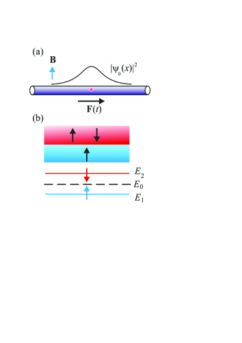
Figure 1: (a) A schematic layout of a shallow donor state formed in a quantum wire. The vectors $\mathbf{B}$ and ${\mathbf{F}}(t)$ show the directions of applied constant magnetic field and periodic electric field, respectively. (b) Scheme of the Zeeman doublet $E_{1}$, $E_{2}$ and the continuum states shown in the shaded bands.

We consider a narrow nanowire, elongated along the $x-$ axis, as shown in Fig. 1(a), where full three-dimensional (3D) electron wavefunction $\psi_{\rm 3D}(\mathbf{r})$ can be presented as a product $\psi_{\rm 3D}(\mathbf{r})=\psi_{\rm 2D}(\mathbf{r}_{\perp})\Psi(x,t).$ Here $\psi_{\rm 2D}(\mathbf{r}_{\perp})$ corresponds to the ground state of the transverse motion with $\mathbf{r}_{\perp}=(y,z),$ and we will be interested only in the motion along the wire described by $\Psi(x,t).$

To characterize this one-dimensional motion, we begin with the following Hamiltonian using the effective mass approximation:

$$H_{0}=\frac{p^{2}}{2m}-\frac{U_{0}}{\cosh^{2}(x/d)},$$ (1)

where the confinement by the donor is described as a potential with the effective width $d$ and the maximum depth $U_{0}$, $m$ is the electron effective mass, and $p=-i\hbar\partial/\partial x\equiv\hbar k$ is the momentum operator. We are interested here in shallow potentials satisfying condition of weak binding such as $\hbar^{2}/md^{2}\gg U_{0}.$ In general, in such potentials the binding energy $E_{0}$ is determined by $E_{0}\sim-m(U_{0}d)^{2}/\hbar^{2}.$ Omitting for the moment the spinor structure, we present the ground state wavefunction at distances $|x|\gg d$ in the form Landau :

$$\psi_{0}(x)=\frac{1}{\sqrt{l}}\exp\left(-\left|x\right|/l\right),$$ (2)

with the localization length $l=\sqrt{{\hbar^{2}}/{2m\left|E_{0}\right|}}\gg d.$

Next, we add the Rashba SOC $H_{R}=\alpha\sigma_{y}k$ and the constant magnetic field $\mathbf{B}=(0,0,B)$ (see Fig. 1) creating the Zeeman term in the Hamiltonian, which now takes the following form:

$$H_{1}=H_{0}+\frac{\Delta}{2}\sigma_{z}+\alpha\sigma_{y}k.$$ (3)

Here the Zeeman splitting $\Delta=\mu_{B}gB,$ where $\mu_{B}$ is the Bohr magneton, and $g$ is the electron g-factor. Since we consider a narrow single quantum wire in the ground state transverse mode, we employ the basic form of the Rashba coupling. Description of the Rashba coupling in more complex nanowire systems can be found, e.g., in Refs. [Mireles2001, ; Gelabert2010, ; Zainuddin2011, ; Xu2014, ].

As a result, the ground state of (1) transforms into a Zeeman-split doublet containing the only two localized eigenstates of (3), with spacing $E_{2}-E_{1}$ (see Fig. 1(b)). For $\alpha=0$ and $g<0$ the ground state $E_{1}$ is the spin-up state where the spin is parallel to the magnetic field, and the state $E_{2}$ is the spin-down state. These Zeeman partners may effectively participate in the spin resonance driven by an external periodic electric field applied along the wire, with the frequency $\omega=(E_{2}-E_{1})/\hbar$ and amplitude $F_{0}$, and described as a potential,

$$V(x,t)=eF_{0}x\sin\omega t,$$ (4)

where $e$ is the fundamental charge, being added to the Hamiltonian $H_{1}.$ The reason for this participation is that due to the presence of SOC the eigenstates of (3) contain both spinor components. Therefore, two states with different signs of their $\sigma_{z}$ can still be coupled by the electric field described by the position operator, creating the possibility of the electric dipole spin resonance.

As for the continuum states, they also split into Zeeman doublets as shown in Fig. 1 by arrows in the bands above $E_{1}$ and $E_{2}$. At $\alpha=0$ and $g<0,$ the low-energy part of the continuum has spin up and is non-degenerate. The higher states are twofold degenerate where the spin-up state from the lower Zeeman energy is accompanied by the spin-down state from the higher Zeeman energy described by the eigenvalue set of continuum for $H_{0}$.

In the absence of the spin-orbit coupling, with the increase in the magnetic field, the discrete state $E_{2}$ reaches the bottom of the continuum at the merging field $B_{\rm m}$ satisfying the condition

$$\mu_{B}|g|B_{\rm m}=|E_{0}|,$$ (5)

and transition frequency $\omega=|E_{0}|\times(B/B_{\rm m})/\hbar.$ Below we will consider the fields lower than $B_{\rm m}$ in order to avoid the direct overlap of the discrete and continuum states in the stationary Hamiltonian (3). However, we will see that discrete and continuum states interact dynamically during the evolution driven by periodic electric field, as it will be discussed in the next Sections.

III Spin-orbit coupling as a perturbation

For a qualitative understanding of the electric dipole spin resonance here we will apply the perturbation theory to highlight the effects of SOC and the presence of continuum on the wavefunctions belonging only to the lowest Zeeman-split doublet. We begin by considering the SOC term $\alpha\sigma_{y}k$ in the Hamiltonian (3) as a perturbation, similarly to the approaches of Refs. [Rashba1964a, ; Khaetsky, ]. At $\alpha=0,$ we label the Zeeman-split doublet state as spin-up $(\lambda=1)$ or spin-down $(\lambda=-1)$ state, respectively.

The states of the discrete spectrum have the form:

$$\psi_{0}^{\lambda=-1}=\left[\begin{array}[]{c}0\\ \psi_{0}(x)\end{array}\right],\qquad\psi_{0}^{\lambda=1}=\left[\begin{array}[]{c}\psi_{0}(x)\\ 0\end{array}\right].$$ (6)

The energies of this Zeeman doublet are $E_{0}^{[\lambda]}=E_{0}+\lambda{\Delta}/2,$ and the only shallow localized ground state is $\psi_{0}(x).$ At $\alpha=0$, $E_{0}^{\lambda=1}=E_{1}$ and $E_{0}^{\lambda=-1}=E_{2}.$

The continuum states are modeled by the approximation of extremely far hard walls located at $|x|=L$ with $L\gg l,$ corresponding to the wire length $2L,$ which leads to the set of very densely located levels representing the continuum with required accuracy Lparameter . The spatially odd states representing the continuous spectrum and coupled by the $k$ term to the even localized states are labeled by the discrete index $n$ in our model:

$$\varphi_{n}^{\lambda=-1}=\left[\begin{array}[]{c}0\\ \varphi_{n}(x)\end{array}\right],\qquad\varphi_{n}^{\lambda=1}=\left[\begin{array}[]{c}\varphi_{n}(x)\\ 0\end{array}\right],$$ (7)

with the above defined energies $E_{n}^{[\lambda]}=E_{n}+\lambda{\Delta}/{2}$ and

$$\varphi_{n}(x)=\frac{1}{\sqrt{L}}\sin\left(k_{n}x\right),$$ (8)

where $E_{n}=\hbar^{2}k_{n}^{2}/2m$ with $k_{n}=\pi n/L.$

When the SOC is turned on, the localized states (6) forming the ground Zeeman doublet acquire the admixture from the continuum states. In the leading order of the perturbation theory one can present them as:

$$\psi^{\lambda=-1}=\left[\begin{array}[]{c}\sum\limits_{n}a_{n}^{\lambda=-1}\varphi_{n}(x)\\ \psi_{0}(x)\end{array}\right],\psi^{\lambda=1}=\left[\begin{array}[]{c}\psi_{0}(x)\\ \sum\limits_{n}a_{n}^{\lambda=1}\varphi_{n}(x)\end{array}\right]$$ (9)

where

$$a_{n}^{[\lambda]}=-\lambda\frac{\alpha}{E_{0}^{[\lambda]}-E_{n}^{[\lambda^{\prime}]}}\int_{-\infty}^{\infty}\varphi_{n}(x)\psi_{0}^{\prime}(x)dx,$$ (10)

and for the wavefunction in Eq. (2) one obtains

$$\int_{-\infty}^{\infty}\varphi_{n}(x)\psi_{0}^{\prime}(x)dx=-\frac{2}{\sqrt{lL}}\frac{k_{n}l}{1+k_{n}^{2}l^{2}}.$$ (11)

By analyzing (10) -(11) one can see that the coefficients $a_{n}^{({\pm})}$ describing the admixture of continuum states for the localized Zeeman-split doublet (9) are proportional to $\alpha.$ This is a simple confirmation of the role played by the continuum states when the SOC is significant. The resulting spin-projected probability to find the electron in the continuum, $w_{\rm c}=\sum_{n}|a_{n}^{[\lambda]}|^{2},$ at $B=0$ is given by $w_{\rm c}=m(\alpha/\hbar)^{2}/|E_{0}|.$

For the following studies of the electric dipole spin resonance we will need the matrix element of coordinate calculated between the states of our interest, that is between $\psi^{\lambda=1}$ and $\psi^{\lambda=-1}$ in Eq. (9). For the localized states (9) with opposite spins one obtains:

$$x_{\lambda\lambda^{\prime}}=\sum_{n}\left(a_{n}^{\lambda=-1}+a_{n}^{\lambda=1}\right)\int_{-\infty}^{\infty}\varphi_{n}(x)x\psi_{0}(x)dx.$$ (12)

Taking into account that

$$\int_{-\infty}^{\infty}\varphi_{n}(x)x\psi_{0}(x)dx=4{\sqrt{\frac{l}{L}}}l\frac{k_{n}l}{(1+k_{n}^{2}l^{2})^{2}},$$ (13)

performing summation over $k_{n}$ and by using (2), (8), and (10), (11), we arrive at

$$x_{\lambda\lambda^{\prime}}=\frac{\alpha}{\left|E_{0}\right|}\frac{1}{\xi^{3}}\left[\xi^{2}+4\left(\sqrt{1-\xi}+\sqrt{1+\xi}-2\right)\right],$$ (14)

with notation $\xi\equiv\Delta/\left|E_{0}\right|=B/B_{\rm m}.$ We consider $|\xi|<1$ to avoid direct overlap of the continuum and localized states, where the energy levels acquire more complicated contributions. By expanding Eq. (14) by $\xi\ll 1$ we obtain $x_{\lambda\lambda^{\prime}}=-5\alpha\xi/16|E_{0}|.$ Note that the matrix element in Eq. (14) can be estimated in terms of two characteristic lengths of the model as $l\times l/l_{\rm so},$ with $l_{\rm so}={\hbar^{2}}/{m\alpha}$ being the spin precession length. While this is the result of the first order perturbation theory which may no longer be applicable for large SOC, it clearly shows the importance of considering the continuum states for the system with shallow donor and strong SOC. Thus, the Zeeman-split discrete states are SOC-coupled via the continuum. This coupling is critical for the driven dynamics which will be analyzed in the next Section.

In a similar way we calculate the energy shift of the state of interest as

$$\Delta E_{\lambda}=-2m\frac{\alpha^{2}}{\hbar^{2}\xi^{2}}\left(\sqrt{1-\lambda\xi}-1\right)^{2}.$$ (15)

In the zero-field limit $\xi\rightarrow 0$ both $\Delta E^{\lambda=-1}$ and $\Delta E^{\lambda=1}$ behave as $-m\left(\alpha/\hbar\right)^{2}/2$ and their difference $\Delta E^{\lambda=-1}-\Delta E^{\lambda=1}\approx m\left(\alpha/\hbar\right)^{2}\xi/2.$ These corrections can be considered as a renormalization of the $g-$factor by the spin-orbit coupling due to the presence of the continuum states and show that the perturbation theory is applicable at $m\left(\alpha/\hbar\right)^{2}/|E_{0}|\ll 1,$ that is at $l\ll l_{\rm so}$ and $|x_{\lambda\lambda^{\prime}}|\ll l.$

IV Spin dynamics for periodic driving

IV.1 Numerical basis states and model of the dynamics

The numerically precise basis states $\phi_{n}$ and the energies $E_{n}^{(0)}$ of the Hamiltonian (1) are found by the discretization on the $x-$ axis. An eigenstate $\psi_{l}(x)$ for (3) with the eigenenergy $E_{l}$ is constructed as a superposition of the basis states $\phi_{n}$ of the Hamiltonian (1) with the coefficients forming the two-component spinors:

$$\psi_{l}(x)=\sum_{n}\left[\begin{array}[]{c}a^{l}_{n}\\ b^{l}_{n}\end{array}\right]\phi_{n}(x).$$ (16)

The spinor coefficients $a_{n}^{l}$ and $b_{n}^{l}$ are found from the numerical diagonalization of (3) with $l=1,\dots,l_{\rm max},$ where $l_{\max}$ is the basis size.

Then, we solve numerically the nonstationary Schrödinger equation

$$i\hbar\frac{\partial}{\partial t}\Psi(x,t)=H(x,t)\Psi(x,t),$$ (17)

with the Hamiltonian $H(x,t)=H_{1}+V(x,t)$, for the time-dependent wavefunction

$$\Psi(x,t)={\bm{C}}^{\rm T}(t)\bm{\psi}(x).$$ (18)

In Eq. (18) ${\bm{C}}(t)$ is the vector with $l_{\rm max}$ components determined from (17), and $\bm{\psi}(x)=\left(\psi_{1}(x),\dots,\psi_{l_{\rm max}}(x)\right)^{\rm T}$. The Hamiltonian in (17) is time-periodic, i.e. $H(x,t)=H(x,t+NT)$ for any integer $N$, where the period $T=2\pi/\omega$. The frequency $\omega$ of the driving field is tuned to match the splitting between the Zeeman doublet of the discrete state, $\hbar\omega=E_{2}-E_{1}$. Since the driving is periodic, we can apply the Floquet technique Jiang2006 ; Reichl ; KGS2012 ; KMSD2013 ; Demikhovskii2002 to obtain the stroboscopic picture of the system state $\Psi(x,t)$ at discrete moments of time $t=NT$ Demikhovskii2002 ; Supplement .

When the wavefunction (18) is found, one can calculate the stroboscopic evolution of various observables such as

$$x(t)=\int_{-\infty}^{\infty}\Psi^{\dagger}(x,t)x\Psi(x,t)dx,$$ (19)

for the position and

$$\sigma_{z}(t)=\int_{-\infty}^{\infty}\Psi^{\dagger}(x,t)\sigma_{z}\Psi(x,t)dx,$$ (20)

for the spin component. We take the initial state $\Psi(x,0)$ as the ground state $E_{1}$ which has the spin component $\sigma_{z}(0)$ close to one. When the first zero of $\sigma_{z}(t)=0$ is achieved (as shown in Fig. 2(a)) during the stroboscopic evolution, we define this time as the half of the “spin-flip” time $T_{\rm{sf}}$. For a few certain values of the system parameters and driving fields it is possible that the condition $\sigma_{z}(t)=0$ is never reached throughout the observation interval. In such a case we define the spin flip rate $1/T_{\rm{sf}}$ as equal to zero.

IV.2 Numerical results

IV.2.1 System parameters

We begin with setting the parameters for numerical calculations. We use a donor state in InSb quantum wire. For InSb the value $m=0.0136m_{0}$ is chosen for the electron effective mass where $m_{0}$ is the mass of a free electron Saidi . We assume $g=-50.6$ for the electron g-factor in InSb. The amplitude of the Rashba SOC $\alpha$ in InSb can be tuned by the gate voltage and can reach high values up to 100 meVnm Leontiadou ; Wojcik .

For the shallow donor parameters we accept $U_{0}=1.5$ meV and $d=10$ nm, as can be realized for a donor screened by a two-dimensional electron gas Ando . As a result, a single discrete level $E_{0}=-0.072$ meV, corresponding to the localization length $l$ close to 200 nm and frequency $|E_{0}|/\hbar\approx 2\pi\times 17.8$ GHz, is formed. All the states with positive energies belong to the continuum. For the chosen parameters Eq. (5) gives the value $B_{\rm m}=25$ mT. We consider three values of magnetic field: $B=0.25B_{\rm m},$ $B=0.5B_{\rm m},$ and $B=0.75B_{\rm m}$ and for each $B$ take two values of SOC: $\alpha=6$ meVnm (for a relatively weak SOC with $l_{\rm so}={\hbar^{2}}/{m\alpha}\approx 10^{3}\mbox{ nm}>l$) and $\alpha=25$ meVnm (for a relatively strong SOC where $l_{\rm so}\approx l$). The basis in Eq. (18), truncated at $l_{\rm max}=250\ldots 500$, provides a good, $l_{\rm max}-$independent, convergence of all the numerical results in the range, where the continuum states are effectively involved in the evolution by the electric fields.

Condition of strong driving field amplitude $F_{s}\sim\left|{E_{0}}/{l}e\right|$ in Eq. (4) yields $\sim 5$ V/cm. Although this value is experimentally accessible, we will limit our calculations to lower fields to avoid a nonlinear, strongly beyond the Fermi’s golden rule, ionization process Delone . Indeed, the semiclassical tunneling probability for a static field $F_{0}$ per time $\hbar/|E_{0}|$ can be estimated as $\exp(-4F_{s}/3F_{0}),$ and one can introduce as a nominal reference parameter the tunneling ionization time $\tau_{\rm ti}=\hbar/|E_{0}|\times\exp(4F_{s}/3F_{0}).$ Since the electric fields of our interest during the oscillation period are considerably weaker than $F_{s}$ the system is stable against the ionization.

IV.2.2 Time dependence of observables

To demonstrate a typical time dependence of the observables of interest, we show in Fig. 2 two examples of the evolution for mean values $\sigma_{z}(NT)$ and $x(NT)$ for driving fields with $F_{0}=0.5$ V/cm and $F_{0}=1.5$ V/cm, on the time interval $N<200$ of the driving field periods. Other parameters are $B=0.5B_{\rm m}$ and $\alpha=6$ meVnm giving the level splitting $E_{2}-E_{1}=0.035$ meV equal to $\approx 2\pi\times 8.65$ GHz of the driving frequency. It should be mentioned that this splitting includes the Zeeman coupling and the contribution due to the presence of the continuum states, which, at weak SOC is proportional to the square of the Rashba SOC strength (see Eq. (15)). In experiment, the driving frequency can be tuned smootly to match the exact level splitting which may differ from the simple Zeeman term. Note that this frequency, being a reference parameter, and independent of the driving field, does not include the dynamical Stark effect Stark .

It can be seen that at low driving amplitude the dynamics of both spin and coordinate mean values shown in Fig.2 is rather regular, especially for the spin, where it reminds the well-known picture for the Rabi resonance in a two-level system with the frequency close to $e|x_{\lambda\lambda^{\prime}}|F_{0}/\hbar.$ As to the coordinate mean value, it demonstrates the combined drift and oscillations which do not exceed the localization length, being of the order of $40-80$ nm. Thus, for low amplitudes of driving the influence of delocalized continuum states of the nanowire is relatively small both for spin and coordinate dynamics as it can be reduced mostly to the formation of nonzero matrix element of coordinate between localized spin-up and spin-down states.

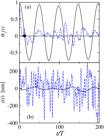
Figure 2: Stroboscopic dynamics for mean values of (a) spin component $\sigma_{z}(t)$ and (b) coordinate $x(t)$ for parameters $B=0.5B_{\rm m}$ and $\alpha=6$ meVnm. The amplitude of the driving electric field $F_{0}=0.5$ V/cm (solid line) and $F_{0}=1.5$ V/cm (dashed line). Black circle in (a) corresponds to $T_{sf}/2$ for $F_{0}=0.5$ V/cm.

The situation changes when the driving amplitude is increased to $F_{0}=1.5$ V/cm. It can be seen that both spin and coordinate loose their simple evolution pattern visible at low driving field. They now demonstrate more complicated dynamics with obviously many states participating in it. This result clearly reflects the presence of continuum states in the driven evolution, which become more significant when the driving amplitude is increased. As to the numerical values in Fig. 2, one can see that the spin projection $\sigma_{z}(t)$ never approaches $-1$, i.e. no full spin flip is achieved. We attribute this effect to the presence of many states with different spin projections and with comparable weights, in the the total wavefunction (18). The coordinate mean value $x(t)$ at a strong driving also demonstrates a complicated and irregularly oscillating behavior, with much greater amplitude than for weak driving, approaching or even exceeding the localization length $l.$ This can be described as another evidence of significant contribution of continuum states in the driven dynamics even for moderate fields less then 3 V/cm.

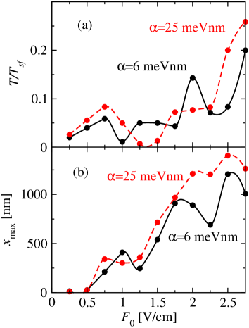
Figure 3: Electric field amplitude dependence of (a) the spin flip rate $1/T_{sf}$ and (b) the maximum displacement $x_{\max}$ for different parameters of the spin-orbit coupling strength $\alpha$ and for $B=0.5B_{\mathrm{m}}:$ (solid lines) $\alpha=6$ meVnm and (dashed lines) $\alpha=25$ meVnm. The lines serve only as the guides for the eye.

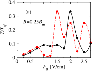
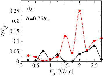
Figure 4: (a) Spin-flip rate for magnetic field $B=0.25B_{\rm m}$. The parameters of the spin-orbit coupling strength are $\alpha=6$ meVnm (solid line) and $\alpha=25$ meVnm (dashed line). (b) Same as in (a) but for higher magnetic field $B=0.75B_{\rm m}$. The lines serve only as the guides for the eye.

IV.2.3 Dependence on the driving field amplitude

It is of interest to track the amplitude characteristics of spin resonance as functions of the driving field amplitude. First of all, we consider the dependence of spin flip rate $1/T_{sf}$ and find it for several values of the field amplitude $F_{0}$ as plotted in Fig.3. Two values of SOC coupling constant are taken for the magnetic field $B=0.5B_{\rm m}$. One can see that for both SOC amplitudes even at a moderate driving field amplitude $F_{0}\approx 0.75$ V/cm, the dependence of $1/T_{sf}$ on $F_{0}$ becomes strongly nonlinear due to the significant role of continuum states in the driven dynamics, taking the system out of a simple two-level approximation. Similar behavior of the spin flip frequency in a multilevel system has been observed in our previous studies of the spin resonance in a double quantum dot KGS2012 . The complicated behavior of coupled spin and charge observables was also observed in a multilevel system represented by a driven two-dimensional quantum billiard with SOC KMSD2013 . One can see in Fig. 3 as well as in Fig. 4 that for certain values of the driving field the spin flip rate decreases to zero. The definition of such case has been discussed at the end of subsection IV.A, and it represents rare cases where the condition $\sigma_{z}(t)=0$ is never reached during the observation time. The main cause of this effect cannot be assigned to the dynamical shift of the resonance condition Delone ; Stark since the significant presence of the continuum states with variable spin projections produces a much more complex coupled spin-position dynamics than that solely caused by a time-dependent Stark effect. This is supported by an observation that the regions with zero $1/T_{\rm{sf}}$ occupy only few intermediate points for driving field amplitudes $F_{0}$ in Figs. 3 and 4. One can see there that an increase in $F_{0}$ generates no results with vanishing $1/T_{\rm{sf}}$ for $F_{0}$ close to the maximum values, so the observed feature is not definitely related to the dynamic energy level shift, which grows with the increasing driving field.

Another characteristic of the driven evolution is the maximum achievable displacement during the total observation time, $x_{\max},$ shown in Fig. 3(b) for the same other parameters as in Fig. 3(a). One may expect that the absolute value $x_{\max}$ grows up monotonically with increasing the electric field strength $F_{0}$. However, strong SOC and the presence of the continuum provide sizable corrections to such a simple estimate, as it can be seen in Fig.3. First of all, the dependence of $x_{\max}$ on $F_{0}$ demonstrates a nonlinear character from the fields of about $1$ V/cm for $\alpha=6$ meVnm and from $0.75$ V/cm for $\alpha=25$ meVnm. For the field amplitude exceeding $F_{0}\approx 1.5$ V/cm, a saturation tendency is clearly visible, indicating that the electric field efficiency in displacing the electron at large distance is strongly reduced.

One can be interested to look at the characteristics of the spin resonance also for other values of the external magnetic field. Here we show the results for the spin flip rate for the field $B=0.25B_{\rm m}$ in Fig. 4 (a) and for $B=0.75B_{\rm m}$ in Fig. 4 (b). As in Fig. 3, for each field we consider two values of the SOC amplitude $\alpha=6$ $\mathrm{meVnm}$ and $\alpha=25$ $\mathrm{meVnm}.$

By analyzing the results in Fig. 3 and Fig. 4, one can conclude that both spin and coordinate dynamics have a lot of common features for different parameters of the magnetic field and SOC. The nonlinear dependence of $1/T_{\rm{sf}}$ and the $x_{\max}$ on the driving field amplitude is clearly visible. The maximum values of $1/T_{\rm{sf}}$ are comparable for all magnetic fields and for all SOC amplitudes. However, it can be seen from Fig. 4(b) that the increase in the magnetic field to $0.75B_{\rm m}$ reduces the SOC-induced coupling between the states with different spin. Indeed, for this field, the values of $1/T_{\rm{sf}}$ are in general lower than those for $B=0.25B_{\rm m}$ and $B=0.5B_{\rm m}$. This finding is especially clear for the low SOC strength $\alpha=6$ meVnm. As one can see in all the Figures, the spin-flip time $T_{\rm{sf}}$ usually does not exceed the nominal tunneling ionization time $\tau_{\rm ti},$ confirming that the time scale of the spin flip process is usually shorter than the time scale of the tunneling ionization.Supplement

The two values of Rashba coupling considered here represent its actual operating range in prospective systems based on InSb nanowires. Indeed, neither very small nor very large SOC is desirable. If the SOC is too weak, the coupling between spin-resolved discrete states via the continuum becomes ineffective. For a very strong coupling one needs large amplitudes $F_{0}$ to flip the spin and to make the qubit actually working since highly mixed spin states are involved and produced by the driving. As a result, a certain range of the SOC strength is needed as represented by these two realizations.

Another key parameter is the driving field amplitude $F_{0},$ limited here by a moderate value of 2.75 V/cm. The first reason for keeping it not very strong is avoiding the nonlinear ionization Delone . The second reason is the absence of an effective increase for the spin flip rate when making the driving amplitude too strong, as it can be seen in Figs. 3 and 4. When the driving is too intense, the continuum states with different spins begin to play more significant role by creating a hardly distinguishable mixture of the two discrete states with the continuum. In such a mixture the spin components together with the wavefunction spread may become poorly defined, prohibiting the application of such a regime for a practically operating qubit. Besides, strong electric fields are in general not desirable for micron- and submicron-sized electronic devices. This is why we restrict ourselves to low and medium driving fields, sufficient for providing an effective operation for the qubit.

Here one additional comment might be of interest. Although the behavior of the driven spin dynamics in the regime of strong spin-orbit coupling is practically unpredictable, some conclusions can be made from the extension of the perturbation theory analysis. In this case, the matrix element of the coordinate $x_{\lambda\lambda^{\prime}}$ is of the order of the localization length $l$. Therefore, the spin-flip Rabi frequency of the order of $eF_{0}l/\hbar$ sets the upper limit on the spin-flip rate for a relatively weak external field, which is confirmed by our results in Fig. 2 for lower amplitude $F_{0}$. For a strong field and a relatively weak spin-orbit coupling, we can conclude from the matrix element on Eq. (13) that the states providing the maximal contribution to (13) and to the spin dynamics have momenta of the order of $\hbar/l$. Therefore, they are described by the precession rate of the order of $\alpha/\hbar l$ that may help to estimate the actual spin-flip rate. However, it can be seen in Figs. 3 and 4 that an increase in the SOC amplitude alone does not lead to the strictly proportional growth of the spin flip rate since the dynamics has a complex nature with many states participating in it.

We note that in all the regimes considered here, $T_{\rm{sf}}$ is of the order of or less than $10T$. Taking into account that $T$ is of the order of 0.1 ns, we find that $T_{\rm{sf}}$ is of the order of a nanosecond. Since the spin relaxation time in week magnetic fields exceeds this time by orders of magnitude Khaetsky ; Amasha , at the time scale of $N\sim 100$, we still have a coherent qubit manipulation in the EDSR regime. Note that the effect of the noise in the electric field always present in the semiconductor system of interest, will not change this result since the spectrum of the noise is not peaked in the frequency range corresponding to the EDSR in the magnetic fields considered in this paper.Li2018

V Conclusions

We studied the electric dipole spin resonance for a nanowire-based donor states coupled to the continuum, the latter playing a critical role in the dynamics. The continuum leads to a strongly nonlinear dependence of the evolution of spin and position on the electric field. The observed characteristics of both spin and position dynamics, having much in common, for different values of magnetic field and spin-orbit coupling, can be of interest for designing novel types of spin and charge qubits when the confining potentials are shallow, and the discrete states strongly interact with the continuum during the qubit operation. For this reason, these effects should be taken into account for possible applications of materials with strong spin-orbit coupling such as InSb for fabricating the qubit-processing structures.

References

- (1) E. I. Rashba, Sov. Phys. Solid State 2, 1109 (1960).
- (2) G. Bemski, Phys. Rev. Lett. 4, 62 (1960).
- (3) R. L. Bell, Phys. Rev. Lett. 4, 52 (1962).
- (4) Y.A. Bratashevskii, A.A. Galkin, and Y.M. Ivanchenko, Sov. Phys. Solid State 5, 260 (1963).
- (5) E. I. Rashba and V.I. Sheka, Sov. Phys. Solid State 6, 114 (1964).
- (6) E. I. Rashba and V.I. Sheka, Sov. Phys. Solid State 6, 451 (1964).
- (7) E. I. Rashba and Al. L. Efros, Phys. Rev. Lett. 91, 126405 (2003).
- (8) J. Ibaez-Azpiroz, A. Eiguren, E. Ya. Sherman, and A. Bergara, Phys. Rev. Lett. 109, 156401 (2012); J. Ibaez-Azpiroz, A. Bergara, E. Ya. Sherman, and A. Eiguren, Phys. Rev. B 88, 125404 (2013).
- (9) A. F. Sadreev and E. Ya. Sherman, Phys. Rev. B 88, 115302 (2013).
- (10) K. C. Nowack, F. H. L. Koppens, Yu. V. Nazarov, and L. M. K. Vandersypen, Science 318, 1430 (2007).
- (11) X. Hu, Yu-xi Liu, and F. Nori, Phys. Rev. B 86, 035314 (2012).
- (12) V. N. Golovach, M. Borhani, and D. Loss, Phys. Rev. B 74, 165319 (2006).
- (13) J. H. Jiang, M. Q. Weng, and M. W. Wu, J. Appl. Phys. 100, 063709 (2006).
- (14) M. Borhani and X. Hu, Phys. Rev. B 85, 125132 (2012).
- (15) M. P. Nowak, B. Szafran, and F. M. Peeters, Phys. Rev. B 86. 125428 (2012).
- (16) J. Romhányi, G. Burkard, and A. Pályi, Phys. Rev. B 92, 054422 (2015).
- (17) Y. Ban, Xi Chen, E. Ya. Sherman, and J. G. Muga, Phys. Rev. Lett. 109, 206602 (2012).
- (18) M. T. Veszeli and A. Pályi, Phys. Rev. B 97, 235433 (2018).
- (19) Rui Li, J. Q. You, C. P. Sun, and F. Nori, Phys. Rev. Lett. 111, 086805 (2013); Rui Li and J. Q. You, Phys. Rev. B 90, 035303 (2014).
- (20) S. Nadj-Perge, S. M. Frolov, E. P. A. M. Bakkers, and L. P. Kouwenhoven, Nature (London) 468, 1084 (2010).
- (21) E. N. Osika and B. Szafran, J. Phys.: Condens. Matter 27, 435301 (2015).
- (22) Y. Oreg, G. Refael, and F. von Oppen, Phys. Rev. Lett. 105, 177002 (2010).
- (23) A. Das, Y. Ronen, Y. Most, Y. Oreg, M. Heiblum, and H. Shtrikman, Nat. Phys. 8, 887 (2012).
- (24) P. W. Brouwer, M. Duckheim, A. Romito, and F. von Oppen, Phys. Rev. Lett. 107, 196804 (2011).
- (25) W. DeGottardi, D. Sen, S. Vishveshwara, Phys. Rev. Lett. 110, 146404 (2013).
- (26) I. Adagideli, M. Wimmer, and A. Teker, Phys. Rev. B 89, 144506 (2014).
- (27) A. Pitanti, D. Ercolani, L. Sorba, S. Roddaro, F. Beltram, L. Nasi, G. Salviati, and A. Tredicucci, Phys. Rev. X 1, 011006 (2011).
- (28) X. Linpeng, T. Karin, M. V. Durnev, R. Barbour, M. M. Glazov, E. Ya. Sherman, S. P. Watkins, S. Seto, and Kai-Mei C. Fu, Phys. Rev. B 94, 125401 (2016); X. Linpeng, M. L. K. Viitaniemi, A. Vishnuradhan, Y. Kozuka, C. Johnson, M. Kawasaki, and Kai-Mei C. Fu, arXiv:1802.03483.
- (29) L. D. Landau and E. M. Lifshitz, Quantum Mechanics - Nonrelativistic Theory, 3rd ed., Course of Theoretical Physics Vol. 3 (Elsevier, 1977).
- (30) F. Mireles and G. Kirczenow, Phys. Rev. B 64, 024426 (2001).
- (31) M. M. Gelabert, L. Serra, D. Sánchez, and R. López, Phys. Rev. B 81, 165317 (2010).
- (32) A. N. M. Zainuddin, S. Hong, L. Siddiqui, S. Srinivasan, and S. Datta, Phys. Rev. B 84, 165306 (2011).
- (33) L. Xu, Xin-Qi Li, and Qing-feng Sun, Sci. Rep. 4, 7527 (2014).
- (34) A. V. Khaetskii and Yu. V. Nazarov, Phys. Rev. B 64, 125316 (2001).
- (35) One can estimate the number of continuum states occupying the typical energy interval of the order of as This inequality assures a large density of the extended states and represent a validity approximation for the continuum. In our numerical studies we took this which gave us a reliable approach for the continuum states.
- (36) L. E. Reichl, The Transition to Chaos. Conservative Classical Systems and Quantum Manifestations, 2nd Ed., Springer-Verlag, New York, 2004.
- (37) D. V. Khomitsky, L. V. Gulyaev, and E. Ya. Sherman, Phys. Rev. B 85, 125312 (2012).
- (38) D. V. Khomitsky, A. I. Malyshev, E. Ya. Sherman, and M. Di Ventra, Phys. Rev. B 88, 195407 (2013).
- (39) V. Ya. Demikhovskii, F. M. Izrailev, and A. I. Malyshev, Phys. Rev. E 66, 036211 (2002); V. Ya. Demikhovskii, F. M. Izrailev, and A. I. Malyshev, Phys. Rev. Lett. 88, 154101 (2002).
- (40) See Supplemental Material for details of stroboscopic approach and short-time dynamics.
- (41) I. Saïdi, S. Ben Radhia, and K. Boujdaria, J. Appl. Phys. 107, 043701 (2010).
- (42) M. A. Leontiadou, K. L. Litvinenko, A. L. Gilbertson, C. R. Pidgeon, W. R. Branford, L. F. Cohen, M. Fearn, T. Ashley, M. T. Emeny, B. N. Murdin, and S. K. Clowes, J. Phys.: Condens. Matter 23, 035801 (2011).
- (43) P. Wójcik, A. Bertoni, and G. Goldoni, Phys. Rev. B 97, 165401 (2018).
- (44) T. Ando, A. B. Fowler, and F. Stern, Rev. Mod. Phys. 54, 437 (1982).
- (45) N. B. Delone and V. P. Krainov, Atoms in Strong Light Fields, (Springer Series in Chemical Physics), Heidelberg (1985).
- (46) In the absence of the SOC, in a weak static electric field both spin-split localized states experience a Stark shift as can be found by perturbation theory using Eq. (13). Their second-order in Stark-originated splitting is then of the order of As a result, for the set of magnetic fields of our interest, the direct effect of the relative Stark shift compared to the effective Zeeman splitting becomes important if both the driving field and the spin-orbit coupling are relatively strong.
- (47) S. Amasha, K. MacLean, Iuliana P. Radu, D. M. Zumbühl, M. A. Kastner, M. P. Hanson, and A. C. Gossard, Phys. Rev. Lett. 100, 046803 (2008).
- (48) A discussion of a frequency-dependent noise can be found in: R. Li, Journ. of Phys.: Cond. Mat. 30, 395304 (2018).