Fermions Tunneling and Quantum Corrections for Quintessencial Kerr-Newman-AdS Black Hole

Abstract

This paper is devoted to study charged fermion particles tunneling through the horizon of Kerr-Newman-AdS black hole surrounded by quintessence by using Hamilton-Jacobi ansatz. In our analysis, we investigate Hawking temperature as well as quantum corrected Hawking temperature on account of generalized uncertainty principle. Moreover, we discuss the effects of correction parameter $\beta$ on the corrected Hawking temperature $T_{e-H}$, graphically. We conclude that the temperature $T_{e-H}$ vanishes when $\beta=100$, whereas for $\beta<100$ and $\beta>100$, the temperature turns out to be positive and negative, respectively. We observe that the graphs of $T_{e-H}$ w.r.t. quintessence parameter $\alpha$ exhibit behavior only for the particular ranges, i.e., $0<\alpha<1/6$, charge $0<Q\leq 1$ and rotation parameter $0<a\leq 1$. For smaller and larger values of negative $\Lambda$, as horizon increases, the temperature decreases and increases, respectively.

Keywords: Quantum tunneling; Dirac equation; GUP; Quantum corrections. PACS numbers: 04.70.Dy; 04.70.Bw; 04.60.-m

1 Introduction

Hawking radiation is the black-body radiation emitted by a black hole (BH) due to quantum effects near the horizon of a BH [1]. It is named after the physicist Stephen Hawking $(1979)$ who derived a theoretical argument for its existence [2]. Hawking with his collaborators [3] studied quantum mechanical uncertainty principle and observed that the rotating BH should create and emit quantum particles. While, the base of BH thermodynamics is propounded by Bekenstein [4], who predicted that the BH must have a finite entropy.

There are various methods to investigate the imaginary part of outward radiated particles action. One of the tunneling method is named as null geodesic method utilized by Parik and Wilczek [5, 6], which is the extension of the analysis of Kraus and Wilczek [7]. They studied the tunneling of massless scalar particles. For an outgoing massive particle, the equation of motion is different from that of massless particle. The trajectory of a massless particle is a null geodesic. Another technique to investigate BH’s tunneling process is Hamilton-Jacobi ansatz introduced by Agheben et al. [8], which is the extension of complex route analysis of Padmanabhan et al. [9].

Later, Kerner and Mann [10] investigated tunneling process of fermion particles by using Hamilton-Jacobi technique and obtained the corresponding Hawking temperature. This phenomenon is based on the calculations of imaginary part of action at horizon which in turn is associated with the Boltzmann factor of emission at Hawking temperature. Also, they [11] investigated fermions tunneling from Rindler and typical non-rotating BH horizons. The WKB approximation is used to investigate the tunneling probability for classically forbidden trajectory from interior to exterior region through horizon. The expression of the tunneling probability $\Gamma$ is given by

$$\Gamma=\exp[-\frac{2}{\hbar}ImI],$$ (1.1)

where I is the semi-classical action of the outgoing particle and $\hbar$ is Planck’s constant.

Black holes are effective modes to explore the effects of quantum gravity by investigating their thermodynamical properties. Using generalized uncertainty principle (GUP) for BH physics, some thrilling implications and consequences have been performed in literature [12]-[14]. Nozari and Saghafi [15] discussed Hawking radiation for massless scalar particles in the background geometry of Schwarzschild BH by following the Parikh-Wilczek tunneling technique and recovered the tunneling rate as well as corrected Hawking temperature by considering GUP. Kerner et al. [16], Li et al. [17] and Jian et al. [18] investigated the tunneling phenomenon of fermions from the Kerr and Kerr-Newman BHs by applying the WKB approximation to the Dirac equation. Using Hamilton-Jacobi ansatz, the GUP-deformed corrected Hawking temperatures for fermions are derived for various curved spacetimes [19]-[27].

By taking into account the quantum corrections and back-reaction effects, Singleton et al. [28, 29] studied the information loss paradox, conservation of energy and entropy. Banerjee and Majhi [30] studied the Hawking radiation process by using quantum tunneling phenomenon at horizons and investigated the back-reaction effects. The quantum tunneling spectrum for scalar and fermion particles has also been discussed in literature [31]-[35].

Using Kerner and Mann’s formulation, Sharif and Javed [36] studied the fermions tunneling phenomenon to investigate Hawking temperatures for charged anti-de Sitter BHs, charged torus-like BHs, $Pleba\acute{n}ski-Demia\acute{n}ski$ family of BHs, regular BHs and traversable wormholes. They [37] also discussed Hawking radiation for a pair of charged accelerating and rotating BHs involving NUT parameter. Moreover, they [38] investigated quantum corrections for regular BHs, i.e., Bardeen and ABGB BHs. Recently, Javed et al. [39] discussed charged vector particles tunneling for a pair of accelerating and rotating BHs as well as for 5D gauged super-gravity BHs.

During $1990$’s, it is observed that the universe is filled with matter and the appealing power of gravity, which pulls all matter together. Later, the Hubble space telescope perceptions for extremely far off supernovae demonstrated that quite a while prior, the universe was really expending more gradually than it is today. So, the expansion of universe has not been slow due to gravity, but it is accelerating. Eventually scholars thought that possibly it was a consequence of Einstein’s hypothesis of gravity, known as cosmological constant $(\Lambda)$. Initially, $\Lambda$ is added by Einstein as a steady term in his field equations of General Relativity in order to study the static universe, later this effort was unsuccessful due to Hubble’s observations, which confirmed that our universe is expanding [40]. Recently, $\Lambda$ is considered as a source term in the field equations, which can be considered as mass of empty space or vacuum energy, adequately utilizing dark energy to adjust gravity [41].

The value of $\Lambda$ could be either positive or negative as per background geometry. Dark energy is gravitationally repulsive, not attractive. The nature of dark energy is still not well understood but detected by its effects on the rate at which universe expand. The idea of dark energy is more theoretical and numerous things are still remain as matter of consideration [42]. Dark energy as a transient vacuum energy resulting from the potential energy of a dynamical field, is known as quintessence. This form of dark energy varies in space and time and distinguished from $\Lambda$. It plays a vital role in the expansion theory of big bang [43].

The description of dark energy in terms of negative cosmological constant (AdS space) has already been discussed in literature. Xu and Wang [44] investigated Kerr-Newman BH solution in the background of quintessential field by utilizing the Newman-Janis algorithm. It is well known fact that the Newman-Janis algorithm does not deal with the cosmological constant, so they extended the solution of Kerr-Newman metric to the Kerr-Newman-AdS solution surrounded by the quintessential dark energy through direct computations satisfying Einstein Maxwell field equations in the background of quintessential matter with negative cosmological constant. Also, they analyzed the singularity of Kerr-Newman AdS BH in the presence of quintessential field which is similar as the case of Kerr BH.

In our analysis, the quintessential field has an equation of state

$$p=\omega\rho,$$

where $\rho$ and $p$ denote the energy density and pressure, respectively. While $\omega$ represents the state parameter having range, $-1<\omega<-1/3$ [44]. For the given AdS BH which is surrounded by quintessential field, their exist two cosmological horizons [45]. As $\omega\rightarrow-1$, the effects of quintessence and cosmological constant will be similar [46]. Moreover, the $PV$ criticality and thermodynamical properties (pressure, volume and Hawking temperature) of quintessential RN-AdS BH is discussed by Li [47].

In our analysis, we are going to extend the work of Xu and Wang in order to investigate the thermodynamical properties of Kerr-Newman-AdS BH in the presence of quintessential field for fermion particles. For this purpose, we have considered quantum tunneling phenomenon of Hawking radiation to investigate Hawking temperature at BH’s horizon as well as its modified quantum corrected form by utilizing Hamilton-Jacobi ansatz. Moreover, we investigate the effects of quintessential field on BH’s thermodynamics. The main purpose of this paper is to investigate Hawking temperature from different aspects for AdS BH in the background of quintessential field incorporating quantum effects. Moreover, we observe the graphical behavior of corrected Hawking temperature with respect to horizon ($r_{+}$) and quintessence parameter for correction parameter ($\beta$) and cosmological constant.

The paper is outlined as follows: In Section 2, we introduce metric of the Kerr-Newman-AdS BH surrounded by the quintessence. In Section 3, we investigate the Hawking radiation phenomenon for charged fermion particles for the above mentioned BH and recoup the tunneling probability and Hawking temperature. By utilizing the modified Dirac equation incorporating GUP, the corrected Hawking temperature is determined in section 4, while section 5 provides entropy corrections. Section 6 consists of the graphical analysis of quantum corrected Hawking temperature, where we study the effects of $\beta$ and $\Lambda$ in detail. The last section contains concluding remarks.

2 Kerr-Newman-AdS BH with Quintessence

The accelerating expansion of the universe implies the crucial contribution of matter with negative pressure in the evolution of universe. This expansion could also be the result of cosmological constant or quintessence matter. If quintessence matter exists all over the universe, it can also be around a BH. Kerr BH has many interesting properties distinct from its non-spinning counterpart, i.e., Schwarzschild BH. Newman and Janis [48]-[51] analyzed that the Kerr metric [52] could be obtained from the Schwarzschild metric using a complex transformation within the framework of the Newman-Penrose formalism [53]. A similar procedure was applied to the Reissner-Nordstrom metric to generate Kerr-Newman metric [54]. The Newman-Janis algorithm proved to be prosperous in generating new stationary solutions of the Einstein field equations [55]-[58]. Zhaoyi and Wang [44] derived the Kerr-Newman-AdS solution in the presence of quintessence by using Newman-Janis algorithm and complex computations.

The line-element can be written as [44]

$$ds^{2} = \frac{\Sigma^{2}}{\Delta_{r}}dr^{2}+\frac{\Sigma^{2}}{\Delta_{\theta}}d\theta^{2}+\frac{\Delta_{\theta}\sin^{2}\theta}{\Sigma^{2}}\left(a\frac{dt}{\Xi}-(r^{2}+a^{2})\frac{d\phi}{\Xi}\right)^{2}$$ (2.1)

$$- \frac{\Delta_{r}}{\Sigma^{2}}\left(\frac{dt}{\Xi}-a\sin^{2}\theta\frac{d\phi}{\Xi}\right)^{2},$$

where

$$\Delta_{r} = R^{2}\left(1-\frac{r^{2}}{\ell^{2}}\right)+Q^{2}-2Mr-\alpha r^{1-3\omega},~{}~{}~{}\Delta_{\theta}=1+\frac{a^{2}\cos^{2}\theta}{\ell^{2}},$$

$$R^{2} = r^{2}+a^{2},~{}~{}~{}\ell^{2}=\frac{3}{\Lambda},~{}~{}~{}\Xi=1+\frac{a^{2}}{\ell^{2}},~{}~{}~{}\Sigma^{2}=r^{2}+a^{2}\cos^{2}\theta.$$

In above expressions, $M$ is BH mass, $Q$ is BH charge defined as $Q^{2}=q_{e}^{2}+q_{m}^{2}$, while $q_{e}^{2}$ and $q_{m}^{2}$ are being electric and magnetic charge parameters, respectively, $a$ is the rotation parameter, $\ell$ is the curvature radius represented by cosmological constant $\Lambda<0$, whereas $\alpha$ is the quintessence parameter and the state parameter $\omega$ ranges from $-1<\omega<-\frac{1}{3}$.

For $\Lambda=0$, the relationship between $\alpha$ and $\omega$ is defined as follows [44]

$$\alpha\leq\frac{2}{(1-3\omega)}8^{\omega}.$$ (2.2)

It is important to note that only for the fixed value of the state parameter $\omega=-2/3$, one can obtain four horizons, these are, inner, outer and two cosmological horizons $r_{q}$ (determined by the quintessence) and $r_{c}$ (influenced by the cosmological constant). For $\omega=-\frac{2}{3}$, the above expression (2.2) implies $\alpha\leq\frac{1}{6}$. For $\Lambda\neq 0$, four roots can be obtained by taking $\Delta_{r}=0$. For $\omega=-\frac{2}{3}$, the horizon equation will become

$$r^{4}+\frac{3\alpha}{\Lambda}r^{3}+\left(a^{2}-\frac{3}{\Lambda}\right)r^{2}+\frac{6M}{\Lambda}r-\frac{3}{\Lambda}\left(a^{2}+Q^{2}\right)=0.$$ (2.3)

The above fourth order algebraic equation can be expressed in terms of its roots, i.e.,

$$(r-r_{in})(r-r_{out})(r-r_{q})(r-r_{c})=0,$$ (2.4)

where, $r_{-}$ is a cauchy (inner) horizon, $r_{+}$ is the event (outer) horizon, $r_{q}$ and $r_{c}$ are two cosmological horizons.

The line-element (2.1) can be expressed as

$$ds^{2}=-f(r,\theta)dt^{2}+\frac{1}{g(r,\theta)}dr^{2}+\frac{1}{\rho(r,\theta)}d\theta^{2}+K(r,\theta)d\phi^{2}-2H(r,\theta)dtd\phi,$$ (2.5)

where the metric functions are defined by

$$f(r,\theta) = \frac{-a^{2}\sin^{2}\theta\Delta_{\theta}+\Delta_{r}}{\Sigma^{2}\Xi^{2}},~{}~{}~{}H(r,\theta)=\frac{a\sin^{2}\theta(-\Delta_{r}+R^{2}\Delta_{\theta})}{\Sigma^{2}\Xi^{2}},$$

$$K(r,\theta) = \frac{\sin^{2}\theta(\Delta_{\theta}R^{4}-a^{2}\sin^{2}\theta\Delta_{r})}{\Sigma^{2}\Xi^{2}},~{}~{}~{}g(r,\theta)=\frac{\Delta_{r}}{\Sigma^{2}},~{}~{}~{}\rho(r,\theta)=\frac{\Delta_{\theta}}{\Sigma^{2}}.$$

The electromagnetic vector potential $A_{\mu}$, is given by [59]

$$A_{\mu}=\frac{1}{\Sigma^{2}\Xi}\left[-(q_{e}r+aq_{m}\cos\theta)dt+(a\sin^{2}\theta q_{e}r+q_{m}R^{2}\cos\theta)d\phi\right].$$ (2.6)

The angular velocity is defined as [60]

$$\Omega=-\frac{g_{t\phi}}{g_{\phi\phi}}=\frac{a(R^{2}\Delta_{\theta}-\Delta_{r})}{R^{4}\Delta_{\theta}-a^{2}\sin^{2}\theta\Delta_{r}},$$ (2.7)

at horizon it can be expressed as [37]

$$\Omega_{H}=\frac{H(r_{+},\theta)}{K(r_{+},\theta)}=\frac{a}{r^{2}_{+}+a^{2}}.$$ (2.8)

The inverse of $f(r,\theta)$ can be written as [37]

$$F(r,\theta)=f(r,\theta)+\frac{H^{2}(r,\theta)}{K(r,\theta)}=\frac{\Delta_{r}\Delta_{\theta}\Sigma^{2}(r,\theta)}{\Xi^{2}(R^{4}\Delta_{\theta}-a^{2}\sin^{2}\theta\Delta_{r})}.$$ (2.9)

3 Charged Fermions Tunneling

This section is devoted to investigate massive charged fermions tunneling phenomenon for Kerr-Newman-AdS BH surround by quintessence having electric and magnetic charges. For this purpose, we will consider the covariant Dirac equation, given as [37]

$$\iota\gamma^{\mu}\left(D_{\mu}-\frac{\iota q}{\hbar}A_{\mu}\right)\Psi+\frac{m}{\hbar}\Psi=0,~{}~{}~{}\mu=0,1,2,3$$ (3.1)

where $q$ is electric charge and $\Psi$ is wave function, while

$$D_{\mu}=\partial_{\mu}+\Omega_{\mu},~{}~{}~{}\Omega_{\mu}=\frac{1}{2}\iota\Gamma_{\mu}^{\alpha\beta}\Sigma_{\alpha\beta},~{}~{}~{}\Sigma_{\alpha\beta}=\frac{1}{4}\iota[\gamma^{\alpha},\gamma^{\beta}].$$ (3.2)

Here, $\gamma^{\mu}$ satisfies the following identities $[\gamma^{\alpha},\gamma^{\beta}]=-[\gamma^{\beta},\gamma^{\alpha}]$ for $\alpha\neq\beta$ and $[\gamma^{\alpha},\gamma^{\beta}]=0$ for $\alpha=\beta$. Using these relationships as well as the symmetric property of connection symbol $\Gamma_{\mu}^{\alpha\beta}$, we can obtain $\Omega_{\mu}=0$, which yields $D_{\mu}=\partial_{\mu}$. Thus, the given Eq.(3.1) reduces to the following form [37, 61]

$$\iota\gamma^{\mu}\left(\partial_{\mu}-\frac{\iota q}{\hbar}A_{\mu}\right)\Psi+\frac{m}{\hbar}\Psi=0,$$ (3.3)

where Dirac matrices $\gamma^{\mu}$ are

$$\gamma^{t}=\frac{1}{\sqrt{F(r,\theta)}}\gamma^{0},~{}~{}~{}\gamma^{r}=\sqrt{g(r,\theta)}\gamma^{3},~{}~{}~{}\gamma^{\theta}=\sqrt{\rho(r,\theta)}\gamma^{1},$$

$$\gamma^{\phi}=\frac{1}{\sqrt{K(r,\theta)}}\left(\gamma^{2}+\frac{H(r,\theta)}{\sqrt{F(r,\theta)K(r,\theta)}}\gamma^{0}\right),$$

here $\gamma^{c}$’s are for chiral and $\gamma$’s are for Minkowski space, defined as [16]

$$\gamma^{0}=\left({\begin{array}[]{cc}0&I\\ -I&0\\ \end{array}}\right),\gamma^{1}=\left({\begin{array}[]{cc}0&\sigma^{1}\\ \sigma^{1}&0\\ \end{array}}\right),\gamma^{2}=\left({\begin{array}[]{cc}0&\sigma^{2}\\ \sigma^{2}&0\\ \end{array}}\right),\gamma^{3}=\left({\begin{array}[]{cc}0&\sigma^{3}\\ \sigma^{3}&0\\ \end{array}}\right).$$ (3.4)

Here, Pauli sigma matrices $\sigma$’s are defined as

$$\sigma^{1}=\binom{0~{}~{}~{}~{}~{}1}{1~{}~{}~{}~{}~{}0},~{}~{}~{}\sigma^{2}=\binom{0~{}~{}-i}{i~{}~{}~{}~{}~{}0},~{}~{}~{}\sigma^{3}=\binom{1~{}~{}~{}~{}0}{0~{}-1}.$$ (3.5)

Spin particles have two types of spin states, spin-up and spin-down, the corresponding wave functions are defined as, respectively

$$\Psi_{\uparrow}(t,r,\theta,\phi) = \left[{\begin{array}[]{cccc}A(t,r,\theta,\phi)\\ 0\\ B(t,r,\theta,\phi)\\ 0\\ \end{array}}\right]\exp\left[\frac{i}{\hbar}I_{\uparrow}(t,r,\theta,\phi)\right],$$ (3.10)

$$\Psi_{\downarrow}(t,r,\theta,\phi) = \begin{bmatrix}0\\ C(t,r,\theta,\phi)\\ 0\\ D(t,r,\theta,\phi)\end{bmatrix}\exp\left[\frac{i}{\hbar}I_{\downarrow}(t,r,\theta,\phi)\right],$$ (3.11)

where $I_{\uparrow}$ (spin-up) and $I_{\downarrow}$ (spin-down) represent particles action. Here, we discuss only the spin-up case, the spin-down case is similar. Moreover, the particles motion is considered in positive radial direction and the corresponding action can be considered as [37]

$$I_{\uparrow}=-Et+J\phi+R(r,\theta),$$ (3.12)

where $E$ and $J$ represent particles energy and angular momentum, respectively, while $R$ is arbitrary function of $r$ and $\theta$. Using WKB approximation and the ansatz (3.12) for spin-up particles into the Dirac equation with $\iota A=B$ and $\iota B=A$, by applying the Taylor’s expansion near the event horizon, we can obtain the following set of equations, i.e.,

$$- B\left[\frac{-E+\Omega_{H}J-q\left(\frac{q_{e}r+aq_{m}}{(r^{2}_{+}+a^{2})^{2}}\right)}{\sqrt{(r-r_{+})F_{r}(r_{+},\theta)}}+\sqrt{(r-r_{+})g_{r}(r_{+},\theta)}R_{r}(r_{+},\theta)\right]$$

$$+ mA=0,$$

$$- B\left[\frac{\iota}{\sqrt{K(r_{+},\theta)}}\left(J+q\frac{a\sin^{2}\theta q_{e}r_{+}+R^{2}_{+}q_{m}\cos\theta}{\Sigma^{2}(r_{+},\theta)}\right)\right.$$

$$+ \left.\sqrt{\rho(r_{+},\theta)}R_{\theta}(r,\theta)\right]=0,$$

$$+ A\left[\frac{-E+\Omega_{H}J-q\left(\frac{q_{e}r+aq_{m}}{(r^{2}_{+}+a^{2})^{2}}\right)}{\sqrt{(r-r_{+})F_{r}(r_{+},\theta)}}+\sqrt{(r-r_{+})g_{r}(r_{+},\theta)}R_{r}(r_{+},\theta)\right]$$

$$+ mB=0,$$

$$- A\left[\frac{\iota}{\sqrt{K(r_{+},\theta)}}\left(J+q\frac{a\sin^{2}\theta q_{e}r_{+}+R^{2}_{+}q_{m}\cos\theta}{\Sigma^{2}(r_{+},\theta)}\right)\right.$$

$$+ \left.\sqrt{\rho(r_{+},\theta)}R_{\theta}(r,\theta)\right]=0.$$ (3.16)

In the above set of Eqs.(3)-(3.16), the expressions can be defined as

$$F_{r}(r_{+},\theta)=\frac{2\left[r_{+}(1-\frac{a^{2}}{\ell^{2}})-\frac{2r^{3}_{+}}{\ell^{2}}-M-\frac{\alpha(1-3\omega)r^{-3\omega}_{+}}{2}\right](r^{2}_{+}+a^{2}\cos^{2}\theta)}{(r^{2}_{+}+a^{2})^{2}},$$

$$g_{r}(r_{+},\theta) = \frac{\Delta_{r}(r_{+})}{\Sigma^{2}(r_{+},\theta)}=\frac{2\left[r_{+}(1-\frac{a^{2}}{\ell^{2}})-\frac{2r^{3}_{+}}{\ell^{2}}-M-\frac{\alpha(1-3\omega)r^{-3\omega}_{+}}{2}\right]}{(r^{2}_{+}+a^{2}\cos^{2}\theta)}.$$

For $m=0$, it is feasible to extract $\frac{1}{\sqrt{\Sigma(r_{+},\theta)}}$ from Eqs.(3) and (3), to make these equations independent of $\theta$. Moreover, Eqs.(3) and (3.16) have no definite $r$ dependence. It is possible to separate the function $R$. So, near the horizon, the arbitrary function $R(r,\theta)$ can be separated as follows

$$R(r,\theta)=R(r)+\Theta(\theta).$$ (3.17)

Equations (3) and (3.16) provide the same equation for $\Theta$ disregarding of $A$ or $B$. For $m=0$, Eqs.(3) and (3) have two feasible solutions, given below

$$R^{\prime}(r_{+})=R^{\prime}_{+}(r_{+})=\left[\frac{\left\{E-\Omega_{H}J-q\left(\frac{q_{e}r+aq_{m}}{(r^{2}_{+}+a^{2})^{2}}\right)\right\}(r^{2}_{+}+a^{2})}{\Delta_{r}(r_{+})(r-r_{+})}\right],$$ (3.18)

$$R^{\prime}(r_{+})=R^{\prime}_{-}(r_{+})=-\left[\frac{\left\{E+\Omega_{H}J-q\left(\frac{q_{e}r+aq_{m}}{(r^{2}_{+}+a^{2})^{2}}\right)\right\}(r^{2}_{+}+a^{2})}{\Delta_{r}(r_{+})(r-r_{+})}\right],$$ (3.19)

where

$$\Delta_{r}(r_{+})=2\left[r_{+}(1-\frac{a^{2}}{\ell^{2}})-\frac{2r^{3}_{+}}{\ell^{2}}-M-\frac{\alpha(1-3\omega)r^{-3\omega}_{+}}{2}\right],$$

$R_{+}$ and $R_{-}$ represent the radial solution of outgoing and incoming particles action, respectively. Solving for $R_{+}(r_{+})$, Eq.(3.18) implies

$$R_{+}(r_{+})=\int\left[\frac{\left\{E-\Omega_{H}J-q\left(\frac{q_{e}r+aq_{m}}{(r^{2}_{+}+a^{2})^{2}}\right)\right\}(r^{2}_{+}+a^{2})}{\Delta_{r}(r_{+})(r-r_{+})}\right]dr.$$

After integrating the above expression at the pole, we get

$$R_{+}(r_{+})=\pm\iota\pi\frac{\left[E-\Omega_{H}J-q\left(\frac{q_{e}r+aq_{m}}{(r^{2}_{+}+a^{2})^{2}}\right)\right](r^{2}_{+}+a^{2})}{2\left[r_{+}(1-\frac{a^{2}}{\ell^{2}})-\frac{2r^{3}_{+}}{\ell^{2}}-M-\frac{\alpha(1-3\omega)r^{-3\omega}_{+}}{2}\right]}.$$

The above equation implies that

$$ImR_{+}=\pm\pi\frac{\left[E-\Omega_{H}J-q\left(\frac{q_{e}r+aq_{m}}{(r^{2}_{+}+a^{2})^{2}}\right)\right](r^{2}_{+}+a^{2})}{2\left[r_{+}(1-\frac{a^{2}}{\ell^{2}})-\frac{2r^{3}_{+}}{\ell^{2}}-M-\frac{\alpha(1-3\omega)r^{-3\omega}_{+}}{2}\right]}.$$ (3.20)

The tunneling probability in terms of spatial ($\oint p_{r}dr$) and temporal contribution ($\breve{E}\Delta t^{out,in}$) is given as follows [62]-[67]

$$\Gamma=\exp\left[\frac{1}{\hbar}\left(Im(\breve{E}\Delta t^{out})+Im(\breve{E}\Delta t^{in})-Im\oint p_{r}dr\right)\right],$$ (3.21)

where $\oint p_{r}dr=\int p^{+}_{r}dr-\int p^{-}_{r}dr$, whereas $p^{\pm}_{r}=\pm\partial_{r}R$. The spatial contribution can be calculated as

$$\Gamma_{spatial} \propto \exp\left[-\frac{1}{\hbar}Im\oint p_{r}dr\right]$$ (3.22)

$$= \exp\left[-\frac{1}{\hbar}Im\left(\int p^{+}_{r}dr-\int p^{-}_{r}dr\right)\right]$$

$$= \exp\left[-\frac{\pi}{\hbar}\left(\frac{\breve{E}(r^{2}_{+}+a^{2})}{r_{+}(1-\frac{a^{2}}{\ell^{2}})-\frac{2r^{3}_{+}}{\ell^{2}}-M-\frac{\alpha(1-3\omega)r^{-3\omega}_{+}}{2}}\right)\right].$$

The connection between interior and exterior regions of a BH defines the temporal part. For $t\rightarrow t-\frac{\iota\pi}{(2\kappa)}$, we can define the temporal contribution as

$$Im(\breve{E}\Delta t^{out,in})=\frac{-\breve{E}\pi}{(2\kappa)},$$

where

$$\breve{E}=\left[E-\Omega_{H}j-q\left(\frac{q_{e}r+aq_{m}}{(r^{2}_{+}+a^{2})^{2}}\right)\right]$$

and

$$\kappa=\left[\frac{r_{+}(1-\frac{a^{2}}{\ell^{2}})-\frac{2r^{3}_{+}}{\ell^{2}}-M-\frac{\alpha(1-3\omega)r^{-3\omega}_{+}}{2}}{(r^{2}_{+}+a^{2})}\right].$$

Thus, the total temporal rate can be obtained as

$$\Gamma_{temp.} \propto \exp\left[\frac{1}{\hbar}\left(Im(\breve{E}\Delta t^{out})+Im(\breve{E}\Delta t^{in})\right)\right],$$ (3.23)

$$= \exp\left[-\frac{\pi}{\hbar}\left(\frac{\breve{E}(r^{2}_{+}+a^{2})}{r_{+}(1-\frac{a^{2}}{\ell^{2}})-\frac{2r^{3}_{+}}{\ell^{2}}-M-\frac{\alpha(1-3\omega)r^{-3\omega}_{+}}{2}}\right)\right].$$

Using Eq.(3.21), the total tunneling rate at horizon $r=r_{+}$ for $\hbar=1$ is derived as

$$\Gamma=\exp\left[\frac{-2\pi\left[E-\Omega_{H}J-q\left(\frac{q_{e}r+aq_{m}}{(r^{2}_{+}+a^{2})^{2}}\right)\right](r^{2}_{+}+a^{2})}{r_{+}(1-\frac{a^{2}}{\ell^{2}})-\frac{2r^{3}_{+}}{\ell^{2}}-M-\frac{\alpha(1-3\omega)r^{-3\omega}_{+}}{2}}\right].$$ (3.24)

Thus, by utilizing Boltzmann equation

$$\Gamma_{B}=\exp\left[\frac{E-j\Omega_{H}-q\left(\frac{q_{e}r+aq_{m}}{(r^{2}_{+}+a^{2})^{2}}\right)}{T_{H}}\right]$$

the Hawking temperature $T_{H}$ at the horizon $r_{+}$ can be obtained as

$$T_{H}=\left[\frac{r_{+}(1-\frac{a^{2}}{\ell^{2}})-\frac{2r^{3}_{+}}{\ell^{2}}-M-\frac{\alpha(1-3\omega)r^{-3\omega}_{+}}{2}}{2\pi(r^{2}_{+}+a^{2})}\right].$$ (3.25)

The above Hawking temperature for the massive particles case is similar as for massless case for Kerr-Newman-AdS BH with quintessence. Moreover, the results for spin-down particles are similar as for spin-up case with the change of sign. The Hawking temperature is acquired for both cases and we conclude that both spin-up and spin-down particles are radiate with alike rate.

4 Quantum Corrections of $T_{H}$

In this section, we analyze Hawking temperature for massive charged fermions by considering tunneling procedure incorporating quantum gravitational effects. The modified form of Dirac equation (3.1) is given as follows [68]

$$-\gamma^{0}\left(\iota\partial_{0}+\frac{q}{\hbar}A_{0}\right)\Psi=\left(\iota\gamma^{i}\partial_{i}+q\frac{\gamma^{i}}{\hbar}A_{i}+\frac{m}{\hbar}\right)(1+\beta\hbar^{2}\partial_{j}\partial^{j}-\beta m^{2})\Psi,$$ (4.1)

where $i=1,2,3$ signifies the spatial coordinates. Moreover, the correction parameter $\beta$ for the minimal length $M_{f}$ is defined as $\beta=\frac{\beta_{0}}{M^{2}_{f}}$ and $m$ is the mass of fermion particles. The Eq.(4.1) can be rewritten as

$$\left[\iota\gamma^{0}\partial_{0}+q\frac{\gamma^{0}}{\hbar}A_{0}+\iota\gamma^{i}\partial_{i}(1-\beta m^{2})+\iota\gamma^{i}\beta\hbar^{2}(\partial_{j}\partial^{j})\partial_{i}+q\frac{\gamma^{i}}{\hbar}A_{i}(1+\right.$$

$$\left.\beta\hbar^{2}\partial_{j}\partial^{j}-\beta m^{2})+\frac{m}{\hbar}(1+\beta\hbar^{2}\partial_{j}\partial^{j}-\beta m^{2})\right]\Psi=0.$$ (4.2)

Using coordinate transformation, $\varphi=\phi-\Omega$t, where

$$\Omega=\frac{a(\Delta_{\theta}(r^{2}+a^{2})-\Delta_{r})}{(r^{2}+a^{2})^{2}\Delta_{\theta}-\Delta_{r}a^{2}sin^{2}\theta},$$ (4.3)

the line-element (2.1) reduces to the following form

$$ds^{2} = -\frac{\Delta_{r}\Sigma^{2}}{(r^{2}+a^{2})^{2}\Delta_{\theta}-\Delta_{r}a^{2}sin^{2}\theta}dt^{2}+\frac{\Sigma^{2}}{\Delta_{r}}dr^{2}+\frac{\Sigma^{2}}{\Delta_{\theta}}d\theta^{2}$$

$$+ \left(\frac{(r^{2}+a^{2})^{2}\Delta_{\theta}-\Delta_{r}a^{2}sin^{2}\theta}{\Sigma^{2}}\right)sin^{2}\theta d\varphi^{2},$$

which can also be expressed as

$$ds^{2}=-F(r,\theta)dt^{2}+\frac{1}{G(r,\theta)}dr^{2}+\frac{1}{K(r,\theta)}d\theta^{2}+H(r,\theta)d\varphi^{2}.$$ (4.4)

We can choose $\gamma$ matrices in the following form

$$\gamma^{t}=\frac{1}{\sqrt{F(r,\theta)}}\left({\begin{array}[]{cc}\iota&0\\ 0&-\iota\\ \end{array}}\right),~{}~{}~{}\gamma^{r}=\sqrt{g(r,\theta)}\left({\begin{array}[]{cc}0&\sigma^{3}\\ \sigma^{3}&0\\ \end{array}}\right),$$ (4.9)

$$\gamma^{\theta}=\sqrt{K(r,\theta)}\left({\begin{array}[]{cc}0&\sigma^{1}\\ \sigma^{1}&0\\ \end{array}}\right),~{}\gamma^{\varphi}=\frac{1}{\sqrt{H(r,\theta)}}\left({\begin{array}[]{cc}0&\sigma^{2}\\ \sigma^{2}&0\\ \end{array}}\right),$$ (4.14)

where $\sigma$’s are defined by Eq.(3.5). For sake of simplicity, here we discuss the case of spin-up, following the outward radial trajectory. The wave function of spin-up particles is defined as

$$\Psi_{\uparrow}(t,r,\theta,\varphi) = \left[{\begin{array}[]{cccc}A(t,r,\theta,\varphi)\\ 0\\ B(t,r,\theta,\varphi)\\ 0\\ \end{array}}\right]\exp\left[\frac{i}{\hbar}I_{\uparrow}(t,r,\theta,\varphi)\right].$$ (4.19)

The terms $\hbar$, $\beta$, $\partial A$ and $\partial B$ are considered only for the first order, i.e., the higher order contributions are ignored. Using WKB approximation and Eqs.(4.19) and (4.14) in Eq.(4.2), we can obtain the following set of equations

$$-\frac{\iota A}{\sqrt{F(r,\theta)}}(\partial_{t}I)+q\frac{\iota A}{\sqrt{F(r,\theta)}}A_{t}-\sqrt{G(r,\theta)}(1-\beta m^{2})(\partial_{r}I)+(1-\beta m^{2})A$$

$$+B\beta\sqrt{G(r,\theta)}(\partial_{r}I)\left[G(r,\theta)(\partial_{r}I)^{2}+K(r,\theta)(\partial_{\theta}I)^{2}+\frac{1}{H(r,\theta)}(\partial_{\varphi}I)^{2}\right]$$

$$-Am\beta\left[G(r,\theta)(\partial_{r}I)^{2}+K(r,\theta)(\partial_{\theta}I)^{2}+\frac{1}{H(r,\theta)}(\partial_{\varphi}I)^{2}\right]=0,$$ (4.20)

$$\frac{\iota B}{\sqrt{F(r,\theta)}}(\partial_{t}I)-\frac{\iota B}{\sqrt{F(r,\theta)}}A_{t}-A\sqrt{G(r,\theta)}(1-\beta m^{2})(\partial_{r}I)+A\beta\sqrt{G(r,\theta)}$$

$$(\partial_{r}I)\left[G(r,\theta)(\partial_{r}I)^{2}+K(r,\theta)(\partial_{\theta}I)^{2}+\frac{1}{H(r,\theta)}(\partial_{\varphi}I)^{2}\right]+Bm(1-\beta m^{2})$$

$$-mB\beta\left[G(r,\theta)(\partial_{r}I)^{2}+K(r,\theta)(\partial_{\theta}I)^{2}+\frac{1}{H(r,\theta)}(\partial_{\varphi}I)^{2}\right]=0,$$ (4.21)

$$B\left[-\sqrt{K(r,\theta)(1-\beta m^{2})}(\partial_{\theta}I)-\frac{\iota(1-\beta m^{2})}{\sqrt{H(r,\theta)}}(\partial_{\varphi}I)+\beta(\partial_{\theta}I)\sqrt{K(r,\theta)}\right.$$

$$\left.\left\{G(r,\theta)(\partial_{r}I)^{2}+K(r,\theta)(\partial_{\theta}I)^{2}+\frac{1}{H(r,\theta)}(\partial_{\varphi}I)^{2}\right\}+\frac{\iota\beta}{\sqrt{H(r,\theta)}}(\partial_{\varphi}I)\right.$$

$$\left.\left\{G(r,\theta)(\partial_{r}I)^{2}+K(r,\theta)(\partial_{\theta}I)^{2}+\frac{1}{H(r,\theta)}(\partial_{\varphi}I)^{2}\right\}\right]=0,$$ (4.22)

$$A\left[-\sqrt{K(r,\theta)}(1-\beta m^{2})(\partial_{\theta}I)-\frac{\iota(1-\beta m^{2})}{\sqrt{H(r,\theta)}}(\partial_{\varphi}I)+\beta(\partial_{\theta}I)\sqrt{K(r,\theta)}\right.$$

$$\left.\left\{G(r,\theta)(\partial_{r}I)^{2}+K(r,\theta)(\partial_{\theta}I)^{2}+\frac{1}{H(r,\theta)}(\partial_{\varphi}I)^{2}\right\}+\frac{\iota B}{\sqrt{H(r,\theta)}}(\partial_{\varphi}I)\right.$$

$$\left.\left\{G(r,\theta)(\partial_{r}I)^{2}+K(r,\theta)(\partial_{\theta}I)^{2}+\frac{1}{H(r,\theta)}(\partial_{\varphi}I)^{2}\right\}\right]=0.$$ (4.23)

The particle’s action is given by

$$I=-(E-\Omega j)t+R(r)+\Theta(\theta,\varphi).$$ (4.24)

Using Eq.(4.24) in Eqs.(4.20)-(4.23) and by focusing on Eqs.(4.22) and (4.23), we observe that they are similar after dividing by $A$ and $B$, and can be expressed as

$$\left\{\beta G_{r}(r_{+},\theta)R^{\prime 2}+K(r_{+},\theta)\beta J_{\theta}^{2}+\beta H(r_{+},\theta)J_{\varphi}^{2}-(1-\beta m^{2})\right\}$$

$$\times\left[\sqrt{K(r_{+},\theta)}J_{\theta}+\iota\frac{1}{\sqrt{H(r_{+},\theta)}}J_{\varphi}\right]=0,$$ (4.25)

where $R^{\prime}=\partial_{r}R$, $J_{\theta}=\partial_{\theta}\Theta$ and $\partial_{\varphi}=\partial_{\varphi}\Theta$. In Eq.(4.25), $\beta$ indicates the quantum gravity effects so it cannot be considered as zero, thus the term in large bracket equals to zero and provide the solution for $\Theta$. Thus, we can write

$$\left[\sqrt{K(r_{+},\theta)}J_{\theta}+\iota\frac{1}{\sqrt{H(r_{+},\theta)}}J_{\varphi}\right]=0.$$ (4.26)

After removing $A$ and $B$ from Eqs.(4.20) and (4.21), we get the following expression

$$P_{6}(\partial_{r}R)^{6}+P_{4}(\partial_{r}R)^{4}+P_{2}(\partial_{r}R)^{2}+P_{0}=0,$$ (4.27)

where

$$P_{6}=\beta^{2}G^{3}F,$$

$$P_{4}=\beta G^{2}F(m^{2}\beta+2\beta C-2),$$

$$P_{2}=GF\left[(1-\beta m^{2})^{2}+\beta(2m^{2}-2m^{4}\beta-2C+\beta C^{2})\right],$$

$$P_{0}=m^{2}(1-\beta m^{2}-\beta C)^{2}F-(E-\Omega j+qA_{t})^{2},$$

$$C=K(r_{+},\theta)J_{\theta}^{2}+\frac{1}{H(r_{+},\theta)}J_{\varphi}^{2}.$$

From Eq.(4.26), we note that $C=0$. Considering $\beta$ only for the first order, the solution of Eq.(4.27) at horizon provides [69]

$$R(r)=\pm\int\frac{1}{\sqrt{GF}}\sqrt{m^{2}(1-2\beta m^{2})F+(E-\Omega j-qA_{t})^{2}}\times$$

$$\left[1+\beta\left(m^{2}+\frac{(E-\Omega j-qA_{t})^{2}}{F}\right)\right]dr.$$

The above equation implies

$$R(r)=\pm\iota\pi\frac{(r^{2}_{+}+a^{2})(E-\Omega_{H}j-qA_{t})}{\Delta_{r}(r_{+})}(1+\beta\Xi),$$ (4.28)

where

$$\Xi=6m^{2}+\frac{6}{r^{2}+a^{2}\cos^{2}\theta}\left(J^{2}_{\theta}+J^{2}_{\varphi}\csc^{2}\theta\right).$$

The positive/negative signs indicate outgoing/incoming particles. Hence, the tunneling rate [70] of charged fermions across the horizon is calculated as

$$\Gamma = \frac{\Gamma_{(emission)}}{\Gamma_{(absorption)}}=\frac{\exp[-\frac{2}{\hbar}(ImR_{+}+Im\Theta)]}{\exp[-\frac{2}{\hbar}(ImR_{-}+Im\Theta)]}=\exp[-\frac{4}{\hbar}ImR_{+}],$$

$$= \exp\left[\frac{-2\pi\left\{E-\Omega_{H}j-q\left(\frac{q_{e}r+aq_{m}}{(r^{2}_{+}+a^{2})^{2}}\right)\right\}(r^{2}_{+}+a^{2})}{r_{+}(1-\frac{a^{2}}{\ell^{2}})-\frac{2r^{3}_{+}}{\ell^{2}}-M-\frac{\alpha(1-3\omega)r^{-3\omega}_{+}}{2}}\right](1+\beta\Xi).$$

For $\hbar=1$, the corrected Hawking temperature $T_{e-H}$ is

$$T_{e-H} = \left[\frac{r_{+}(1-\frac{a^{2}}{\ell^{2}})-\frac{2r^{3}_{+}}{\ell^{2}}-M-\frac{\alpha(1-3\omega)r^{-3\omega}_{+}}{2}}{2\pi(r^{2}_{+}+a^{2})}\right](1+\beta\Xi)^{-1},$$ (4.29)

$$= T_{\circ}\left[1-\beta\Xi+(\beta\Xi)^{2}+...\right],$$

$$\approx T_{\circ}(1-\beta\Xi).$$ (4.30)

where the semi-classical Hawking temperature is

$$T_{\circ}=\left[\frac{r_{+}(1-\frac{a^{2}}{\ell^{2}})-\frac{2r^{3}_{+}}{\ell^{2}}-M-\frac{\alpha(1-3\omega)r^{-3\omega}_{+}}{2}}{2\pi(r^{2}_{+}+a^{2})}\right].$$

The corrected temperature is based on quantum numbers, i.e., mass, energy and angular momentum.

5 Logarithmic Entropy Corrections

This section is devoted to calculate the entropy corrections for Kerr-Newman-AdS BH with quintessence. Using null geodesic technique, Banerjee and Majhi [30] investigated the corrected Hawking temperature and corrected entropy by taking into account the back-reaction effects. Majhi [32] also analyzed the corrected temperature and entropy by using the first and second laws of thermodynamics. In our investigation, we calculate the entropy corrections for Kerr-Newman-AdS BH involving quintessence by considering the generic formula for leading order corrections to Bekenstein-Hawking formula [71]. It is worth mentioning here that, one could calculate the logarithmic corrections to the BH entropy at inner/outer horizon ($r_{\pm}$) without knowing the values of any specific heat of the BH but only knowing the values of Hawking temperature $(T_{{e-H},{\pm}})$ and entropy ($S_{0,\pm}$), for the given BH. The BH entropy corrections ($S_{\pm}$) can be defined as

$$S_{\pm}=S_{0,\pm}-\frac{1}{2}\ln\mid T^{2}_{e-H,\pm}S_{0,\pm}\mid+...~{}.$$ (5.1)

The classical entropy for given BH at $r=r_{+}$ can be calculated as follows

$$S_{0,+}=\frac{\mathcal{A}_{+}}{4}=\frac{\pi\left(r_{+}^{2}+a^{2}\right)}{\left(1-\frac{a^{2}}{\ell^{2}}\right)},$$ (5.2)

where

$$\mathcal{A}_{+}=\int_{0}^{2\pi}\int_{0}^{\pi}\sqrt{g_{\theta\theta}g_{\phi\phi}d\theta d\phi}.$$

After substituting the corrected Hawking temperature $T_{e-H}$ (given by Eq.(4.30)) in the above Eq.(5.1), we can obtain the logarithmic corrections of entropy in the following form

$$S=S_{0,+}-\frac{1}{2}\ln\left|\frac{\left(r_{+}(1-\frac{a^{2}}{\ell^{2}})-\frac{2r^{3}_{+}}{\ell^{2}}-M-\frac{\alpha(1-3\omega)r^{-3\omega}_{+}}{2}\right)^{2}}{4\pi(r^{2}_{+}+a^{2})\left(1-\frac{a^{2}}{\ell^{2}}\right)}(1-\beta\Xi)^{2}\right|+...$$

This expression represents the corrected entropy for Kerr-Newman-AdS BH involving quintessence parameter.

6 Effects of $\beta$ on $T_{e-H}$

In this section, we analyze graphically the effects of $\beta$ on $T_{e-H}$ with respect to various parameters.

6.1 Temperature $T_{e-H}$ with Horizon $r_{+}$

This subsection is devoted to discuss the behavior of corrected Hawking temperature in different domains of event Horizon $r_{+}$ with fixed BH mass $M=1$, state parameter $\omega=-\frac{2}{3}$ and $\Xi=0.01$.

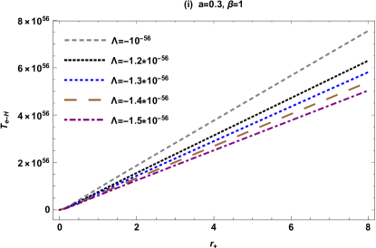
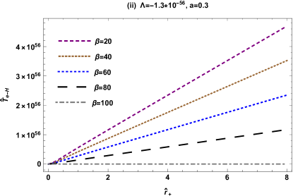
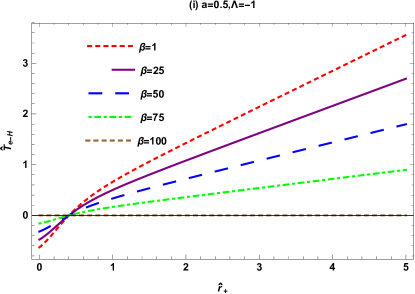
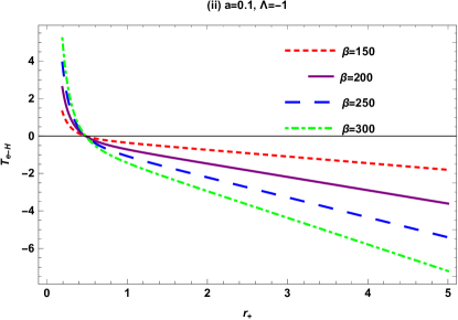
Figure 1: For $\alpha=0.01$, Hawking temperature $T_{e-H}$ with respect to horizon $r_{+}$.

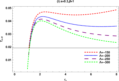
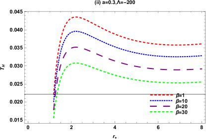
Figure 2: For $\alpha=1$, Relation between the temperature and $r_{+}$.

Figure 3: For $\alpha=1$, Relation between the temperature and $r_{+}$.

• Figure 1 indicates the behavior of Hawking temperature with $r_{+}>0$, for different values of cosmological constant $\Lambda<0$ with fixed values of rotation parameter $a=0.3$ and correction parameter $\beta=1$. The cosmic repulsion indicates that the recent value of the cosmological constant is $\Lambda\approx-1.3\times 10^{-56}cm^{-2}$ [44]. In our analysis, we consider this fixed value of $\Lambda=-1.3\times 10^{-56}cm^{-2}$, as well as we consider $\Lambda$ greater and lesser than this fixed value. (i): For different values of $\Lambda$ near to the fixed value, we can observe that the temperature has its maximum value and its behavior is linear. As horizon increases the temperature also increases. The change in $\Lambda$ defines the diverging temperature $T_{e-H}$ as $r_{+}$ increases. (ii): Indicates the behavior of temperature for fixed values of $a=0.3$ and $\Lambda=-1.3\times 10^{-56}$, while the values of $\beta$ varies. We can observe that for $\beta<100$, the temperature is going to increase as $\beta$ going lesser from $100$. While, for $\beta=100$, the temperature will be zero. The temperature has linear behavior, it increases as horizon increases.

• Figure 2 indicates the behavior of $T_{e-H}$ for fixed values of $a$ and $\Lambda$, while for varying $\beta$. (i): We can observe that for fixed value of $a=0.5$, $\Lambda=-1$ and for varying $\beta<100$, the behavior of temperature is positively increasing $T_{e-H}>0$. While, for $\beta=100$, the graph shows zero temperature, i.e., $T_{e-H}=0$. (ii): For fixed $a=0.1$, $\Lambda=-1$ and for varying $\beta>100$, we observe the negatively divergent behavior of temperature, i.e., the temperature is decreasing as horizon increases in the negative range. This negative and divergent behavior of temperature reflects the non-physical unstable state of BH.

  It is also worth mentioning here that, for the values of correction parameter $1\leq\beta<100$, we observe positive values of temperature and for $\beta=100$, the temperature vanishes, while for $\beta>100$, we observe non-physical behavior with negative temperature.

• Figure 3 shows the behavior of temperature for fixed values of $a=0.3$ and varying $\Lambda$ and $\beta$. (i): We can observe that for $a=0.3$ and $\beta=1$, as $\Lambda$ decreases, the temperature will be small and after attaining its maximum value, the temperature decreases. For $\Lambda\ll 0$, the temperature decreases as horizon increases. In all curves, the temperature has its maximum value at small horizon. The horizon of BH can never be zero, the non-zero value of horizon leads to a BH remnant with maximum temperature.(ii): We observe that for $a=0.3$, $\Lambda=-200$ and for varying $\beta<100$, the temperature attains positive values, Initially, the temperature will be maximum at non-zero horizon and later decreases exponentially as horizon increases, which indicates a physical stable state of BH.

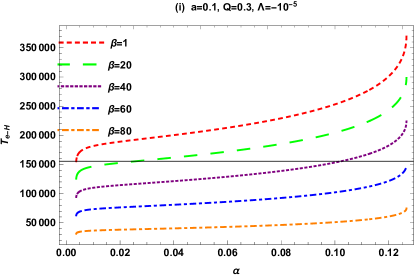
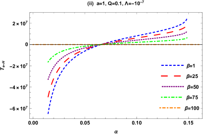
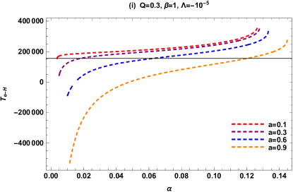
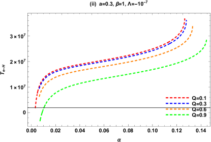
Figure 4: Relation between temperature and $\alpha$ in term of $\beta$.

Figure 5: Relation between temperature and $\alpha$ in term of $a$ and $Q$.

6.2 Temperature $T_{e-H}$ with Quintessence $\alpha$

This subsection gives the analysis of corrected Hawking temperature $T_{e-H}$ with quintessence parameter $\alpha$ for different values of rotation parameters $a$, BH charge $Q$ and cosmological constant $\Lambda$ for fixed $M=1$, $\omega=-\frac{2}{3}$ and $\Xi=0.01$.

• Figure 4 shows the behavior of temperature for fixed $a$, $Q$, $\Lambda$ and for varying $\beta$. (i): We can observe that for fixed values of $a=0.1$, $Q=0.3$, $\Lambda=-10^{-5}$ and for different values of $\beta$, the temperature gradually increases as $\beta$ decreases. It is to be noted that for these parameters, the temperature increases with increase in $\alpha$ as $\beta\rightarrow 1$. (ii): This graph indicates the behavior of temperature for fixed values of $a=1$, $Q=0.1$, $\Lambda=-10^{-7}$ and for varying $\beta$. It is to be noted that for $\beta<100$, the behavior of temperature is from negative to positive, while it attains maximum values and temperature increases with increase in $\alpha$. While, for $\beta=100$, the temperature vanishes, i.e., $T_{e-H}=0$. It is important to note that the both negative and positive behaviors of temperature shows that the initial unstable state of BH, which turns out to be stable with time. This negative temperature is the effect of rotation parameter $a=1$ (maximum value).

• Figure 5 shows the behavior of temperature for fixed $\Lambda$ and $\beta$, while for varying $a$ (in Fig.(i)) and varying $Q$ (in Fig.(ii)). (i): We can observe that for fixed values of $Q=0.3$, $\beta=1$, $\Lambda=-10^{-5}$ and for varying $a$, the temperature gradually increases for increasing $\alpha$. It is to be noted that as $a\rightarrow 1$, the temperature will goes on from negative to positive. (ii): We can observe that for fixed values of $a=0.3$, $\beta=1$, $\Lambda=-10^{-7}$ and for varying $Q$, the temperature will be high enough and it will gradually increase with increase in $\alpha$.

6.3 3D Plots: $T_{e-H}$ and $r_{+}$ with $\Lambda$, $\alpha$ and $\beta$

This section is based on the analysis of Hawking temperature with quintessence parameter $\alpha$, horizon $r_{+}$ and cosmological constant $\Lambda$ for fixed $M=1$, $\omega=-\frac{2}{3}$ and $\Xi=0.01$. This section consists of $3D$ graphs.

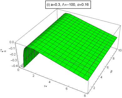
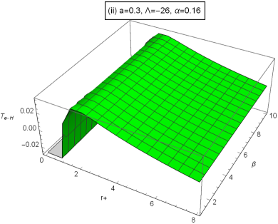
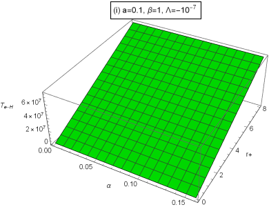
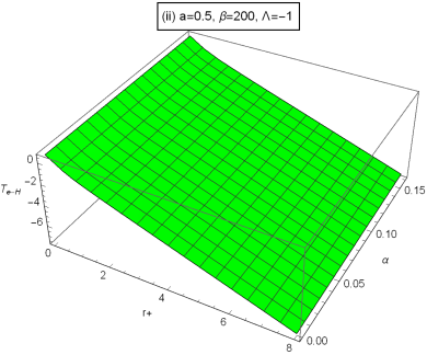
Figure 6: Relation between temperature with $r_{+}$ and $\beta$.

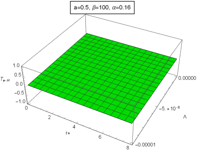
Figure 7: Relation between temperature with $r_{+}$ and $\alpha$.

Figure 8: Relation between temperature with $r_{+}$ and $\Lambda$.

• Figure 6 shows the behavior of temperature for fixed $a$, $\Lambda$ and $\alpha$, while for $\beta<100$. (i): Here, for fixed $a=0.3$, $\Lambda=-100$ and $\alpha=0.16$, the behavior of $T_{e-H}$ indicates that the temperature attains negative values and its behavior is constant w.r.t. $\beta$. After attaining its maximum value at non-zero horizon, the Hawking temperature decreases as horizon increases. This indicate that there exist a BH remnant during the evaporation process. The BH temperature attains its maximum value as horizon shrinks. For $\Lambda=-100$, the temperature is negative for $\beta<100$ and invert for other $\beta$ (already mentioned in $2D$ graphs0. (ii): Graph indicates the behavior of temperature for fixed $a=0.3$, $\Lambda=-26$ and $\alpha=0.16$. We can observe that the behavior of temperature is same as in (i). For $\Lambda=-100$, the temperature is negative but as we increase the value of $\Lambda$ till $\Lambda=-26$, the graph will exhibit the behavior of temperature from negative to positive and for $\Lambda=-25$, the graph will exhibit the positive temperature.

• Figure 7 shows the behavior of $T_{e-H}$ with $r_{+}$ and $\alpha$ for fixed $a$, $\beta$ and $\Lambda$. (i): Graph indicates the behavior of $T_{e-H}$ for fixed $a=0.1$, $\beta=1$ and $\Lambda=-10^{-7}$. We can observe that for larger value of $\Lambda$, the behavior of temperature is linear w.r.t. $r_{+}$. The temperature attains high values and increases with increase in $\alpha$. (ii): This figure indicates the behavior of temperature for fixed $a=0.5$, $\beta=200$ and $\Lambda=-1$. We can observe that as horizon increases the temperature decreases. While for $\alpha$, the temperature increases as $\alpha$ increases. In Fig. 7, the behavior of temperature is same as proved in $2D$ graphs.

• Figure 8 shows the behavior of temperature with horizon $r_{+}$ and cosmological constant $\Lambda$ for fixed $a=0.5$, $\beta=100$ and $\alpha=0.16$. We can observe that for $\beta=100$, the effect of temperature will be zero, as concluded in $2D$ graphs.

It is worth mentioning here that from 2D and 3D graphs, we conclude that the temperature increases with decreasing horizon and increasing $\alpha$. For small values of $\Lambda\neq-100$ and $\beta>100$, the temperature shows negative values. For larger values of $\Lambda$, the temperature will be maximum and its behavior is linear w.r.t. horizon. Moreover, for large $\Lambda$, the temperature increases with increasing $\alpha$.

7 Conclusion

In this paper, we have computed radiation spectrum by analyzing Hawking temperature for Kerr-Newman-AdS BH surrounded by quintessence. For this purpose, we have utilized the WKB approximation and the Hamilton-Jacobi ansatz for massive charged spin-$\frac{1}{2}$ particles (fermions). The investigation yields the corrected Hawking temperature $T_{e-H}$, reliable with BH universality. In our analysis, we have altered the Dirac equation in curved spacetime by incorporating quantum gravity effects through GUP. We have evaluated the tunneling rate at horizon as well as the corresponding Hawking temperature, quantum corrected Hawking temperature as well as quantum corrected entropy. We have analyzed in detail quantum corrected Hawking temperature graphically.

We have summarized the detailed graphical analysis of this paper in the following points:

• The derived Hawking temperature and its modified form $T_{e-H}$ depends on BH’s mass, charge and rotation parameters, as well as on the mass and angular momentum of the emitted fermion particles, quintessence parameter $\alpha$ and state parameter $\omega$.

• When the quantum gravity effects are neglected ($\beta=0$), we have recovered the Hawking temperature of Kerr Newman AdS BH with quintessence. For $\alpha=0$ and $\omega=0$, we have obtained the Hawking temperature of Kerr-Newman AdS BH. Moreover, when $\Lambda=0$, the temperature of Kerr Newman BH has obtained. In addition, for charge-free ($Q=0$) and non-rotating ($a=0$) case, the temperature and its correction reduce to the case of Schwarzschild BH.

• In our analysis, we have considered $\Xi=0.01$, then the condition of GUP must be satisfied for $0<\beta<100$. We have substituted the above mentioned values in Eq.(4.29) for positive values of $T_{\circ}$, the correction terms became smaller than the previous terms given in series. When we consider the first order quantum corrections, the correction term is smaller than $T_{\circ}$. For $\beta=100$, the first order correction term is same as semi-classical term $T_{\circ}$, showed invalidity of GUP. When $\beta>100$, the correction term became greater than the preceding term and the condition of GUP is not satisfied.

• Graphical analysis showed that the behavior of $T_{e-H}$ is positive and negative when $\beta<100$ and $\beta>100$, respectively. While, for $\beta=100$, the temperature vanishes.

• For fixed $\Lambda\approx-1.3\times 10^{-56}$ [44], as well as greater and lesser than this fixed value of $\Lambda$, we have observed that the temperature increases as horizon increases, which is non-physical. The negative as well as divergent behavior of Hawking temperature indicates the behavior reverse to Hawking’s phenomenon, representing unstable state of BH. While, for smaller $\Lambda\ll 0$, the temperature decreases with increasing horizon, which is physical.

• For smaller $\Lambda$, we have obtained physical (stable, +ive $T_{e-H}$) and non-physical (-ive $T_{e-H}$) behavior of temperature for $\beta<100$ and $\beta>100$, respectively.

• We have observed the behavior of $T_{e-H}$ w.r.t. $\alpha$ only for the particular ranges, i.e., $0<\alpha<1/6$, $0<Q\leq 1$, $\Lambda\leq-1$ and $0<a\leq 1$.

• For $T_{e-H}$ w.r.t. $\alpha$, at maximum value of the rotation parameter (i.e., $a=1$), we have observed non-physical and unstable state of BH, which is due to the instability in temperature.

• The results obtained from 3D graphs are similar to the results obtained from 2D graphs.

References

- [1] Hawking, S.W.: Commun. Math. Phys. 43(1975)199; Erratum: Commun. Math. Phys. 46(1976)206.
- [2] Charlie, R.: A conservation with Dr. Stephen Hawking and Lucy Hawking (Archived from the original on March 29, 2013).
- [3] Hawking, S.: A Brief History of Time (Bantam Dell, 1988, United Kingdom).
- [4] Bekenstein, J.: Phys. Rev. D7(1973)2333.
- [5] Parikh, M.K. and Wilczek, F.: Phys. Rev. Lett. 85(2000)5042.
- [6] Parik, M.K.: Phys. Lett. B546(2002)189; ibid. Int. J. Mod. Phys. D13(2004)2351.
- [7] Kraus, P. and Wilczek, F.: Nucl. Phys. B433(1995)403; ibid. Nucl. Phys. B437(1995)231; Kraus, P. and Vakkuri, K.E.: Nucl. Phys. B491(1997)249.
- [8] Agheben, M., Nadalini, M., Vanzo, L. and Zerbibi, S.: JHEP. 0505(2005)014.
- [9] Srinivasan, K. and Padmanabhan, T.: Phys. Rev. D60(1999)24007; Shankaranarayanan, S., Srinivasan, K. and Padmanabhan, T: Mod. Phys. Lett. A16(2001)571; Shankaranarayanan, S., Srinivasan, K. and Padmanabhan, T: Class. Quant. Grav. 19(2002)2671; Shankaranarayanan, S.: Phys. Rev. D67(2003)084026.
- [10] Kerner, R. and Mann, R.B.: Class. Quant. Grav. 25(2008)095014; ibid. Phys. Lett. B665(2008)277.
- [11] Kerner, R. and Mann, R.B.: Fermions Tunneling from Black Holes; arXiv:0710.0612.
- [12] Nozari, K. and Mehdipour, S.H.: JHEP. 0903(2009)061.
- [13] Ali, A.F.: JHEP. 1209(2012)067.
- [14] Majumder, B.: Phys. Lett. B701(2011)384.
- [15] Nozari, K. and Saghafi, S.: JHEP. 11(2012)005.
- [16] Kerner, R. and Mann, R.B.: Phys. Lett. B665(2008)277.
- [17] Li, R., Ren, J.R. and Wei, S.W.: Class. Quantum Gravity 25(2008)125016.
- [18] Jian, T. and Chen, B.B.: Acta physica Polonica B40(2009)241.
- [19] Majumder, B.: Gen. Relativ. Gravit. 45(2013)2403.
- [20] Chen, D.Y., Wu, H.W. and Yang, H.T.: Adv. High Energy Phys. (2013)432412.
- [21] Chen, D.Y., Jiang, Q.Q., Wang, P. and Yang, H.T.: J. High Energy Phys. 11(2013)176.
- [22] Chen, D.Y., Wu, H.W. and Yang, H.T.: J. Cosmol. Astropart. Phys. 03(2014)036.
- [23] Bargueno, P. and Vagenas, E.C.: Phys. Lett. B742(2015)15.
- [24] Mu, B.R., Wang, P. and Yang, H.T.: Adv. High Energy Phys. (2015)898916.
- [25] Wang, P., Yang, H. and Ying, S.: Int. J. Theor. Phys. 55(2016)2633.
- [26] Anacleto, M.A., Brito, F.A. and Passos, E.: Phys. Lett. B749(2015)181.
- [27] Feng, Z.W., Li, H.L., Zu, X.T. and Yang, S.Z.: Eur. Phys. J.C. 76(2016)212.
- [28] Singleton, D., Vagenas, E.C., Zhu, T. and Ren, J.R.: JHEP 1008(2010)089.
- [29] Singleton, D., Vagenas, E.C. and Zhu, T.: JHEP 1405(2014)074.
- [30] Banerjee, R. and Majhi, B.R.: Phys. Lett. B662(2008)62; ibid. JHEP 0806(2008)095; ibid. Phys. Lett. B674(2009)218; ibid. Phys. Rev. D79(2009)064024; ibid. Phys. Lett. B675(2009)243.
- [31] Banerjee, R., Majhi, B.R. and Samanta, S.: Phys. Rev. D77(2008)124035.
- [32] Majhi, B.R.: Phys. Rev. D79(2009)044005; ibid. Phys. Lett. B686(2010)49.
- [33] Majhi, B.R. and Samanta, S.: Annals Phys. 325(2010)2410.
- [34] Banerjee, R., Majhi, B.R. and Vagenas, E.C.: Phys. Lett. B686(2010)279; ibid. Europhys. Lett. 92(2010)20001.
- [35] Bhattacharya, K. and Majhi, B.R.: Phys. Rev. D94(2016)024033.
- [36] Sharif, M. and Javed, W.: Can. J. Phys. 90(2012)903; ibid. Gen. Relativ. Gravit. 45(2013)1051; ibid. Can. J. Phys. 91(2013)43; ibid. J. Exp. Theor. Phys. 115(2012)782; ibid. Proceedings of the 3rd Galileo–Xu Guangqi Meeting, Int. J. Mod. Phys.: Conference Series, 23(2013)271;ibid. Proceedings of the 13th Marcel Grossmann Meeting (Stockholm, 2012), World Scientific, 3(2015)1950.
- [37] Sharif, M. and Javed, W.: Eur. Phys. J. C72(2012)1997.
- [38] Sharif, M. and Javed, W.: J. Korean. Phys. Soc. 57(2010)217.
- [39] Javed, W., Abbas, G. and Ali, R.: Eur. Phys. J. C77(2017)296.
- [40] Longair, M.S.: Confrontation of Cosmological Theories with Observational Data (Springer Science and Business Media, 1974).
- [41] Alex, H.: How Einstein Discovered Dark Energy; arXiv:1211.6338.
- [42] Overbye, D.: Astronomers Report Evidence of Dark Energy Splitting the Universe(The New York Times, August 5,2015).
- [43] Carroll, S.M.: Phys. Rev. Lett. 81(1998)3067.
- [44] Xu, Z. and Wang, J.: Phys. Rev. D95(2017)064015.
- [45] Kiselev, V.V.: Classical Quantum Gravity 20(2003)1187.
- [46] Caldwell, R.R.: Brazilian Journal of Physics 30(2000)2.
- [47] Li, G.Q.: Phys. Lett. B735(2014)256.
- [48] Newman, E.T. and Janis, A.I.: J. Math. Phys. 6(1965)915.
- [49] Newman, E.T., Couch, E., Chinnapared, K., Exton, A., Prakash, A. and Torrence, R.: J. Math. Phys. 6(1965) 918.
- [50] Newman, E.T.: J. Math. Phys. 14(1973)774.
- [51] Newman, E.T.: The Remarkable Efficacy of Complex Methods in General Relativity ed. by B.R. Iyer, et al. Highlights in Gravitation and Cosmology. Proceedings of the International Conference on Gravitation and Cosmology (Goa, 1987), (Cambridge University Press, Cambridge, 1988).
- [52] Kerr, R.P.: Phys. Rev. Lett. D 11(1963) 237.
- [53] Newman, E. and Penrose, R. J. Math. Phys. 3(1962)566.
- [54] Newman, E.T., Couch, E., Chinnapared, K., Exton, A., Prakash, A. and Torrence, R.: J. Math. Phys. 6(1965)918.
- [55] Bambi, C. and Modesto, L.: Phys. Lett. B 721(2013)329.
- [56] Toshmatov, B., Ahmedov, B., Abdujabbarov, A. and Stuchlik, Z.: Phys. Rev. D 89(2014)104017.
- [57] Larranaga, A. and Cardenas, A.A. and Torres, D.A.: Phys. Lett. B743(2015)492.
- [58] Ghosh, S.G. and Maharaj, S.D.: Eur. Phys. J. C75(2015)7 .
- [59] Caldarelli, M.M., Cognola, G. and Klemm, D.: Class. Quant. Grav. 71(2000)399.
- [60] Aliev, A.N.: Phys. Rev. D75(2007)084041.
- [61] Ahmed, J. and Saifullah, K.: JCAP 08(2011)011.
- [62] Akhmedov, E.T., Akhmedova, V. and Singleton, D.: Phys. Lett. B642(2006)124.
- [63] Akmedov, E.T., Akhmedova, V. Pilling, T. and Singleton, D.: Int. J. Mod. Phys. A22(2007)1705.
- [64] Akhmedova, V., Pilling, T., de Gill, A. and Singleton, D.: Phys. Lett. B666(2008)269.
- [65] Akhmedov, E.T., et al.: Int. J. Mod. Phys. D17(2008)2453.
- [66] Akhmedova, V., et al.: Phys. Lett. B666(2008)269; ibid. Phys. Lett. B673(2009)227.
- [67] Gill, d., Singleton, D., Akhmedova, V. and Pilling, T.: Am. J. Phys. 78(2010)685.
- [68] Chen, D., Wu, H., Yang, H. Yang, S.: Int. J. Mod. Phys. A29(2014)1430054.
- [69] Akhmedov, E.T., Pilling, T. and Singleton, D.: Int. J. Mod. Phys. A22(2007)1705; Chowdhury, B.D.: Pramana 70(2008)593; Akhmedov, E.T., Akhmedova, V. and Singleton, D.: Phys. Lett. B642(2006)124.
- [70] Mitra, P.: Phys. Lett. B648(2007)240.
- [71] Pradhan, P.: Adv. High Energy Phys. 2017(2017)2367387.