Importance Sampling-based Transport Map Hamiltonian Monte Carlo for Bayesian Hierarchical Models

Abstract

We propose an importance sampling (IS)-based transport map Hamiltonian Monte Carlo procedure for performing full Bayesian analysis in general nonlinear high-dimensional hierarchical models. Using IS techniques to construct a transport map, the proposed method transforms the typically highly challenging target distribution of a hierarchical model into a target which is easily sampled using standard Hamiltonian Monte Carlo. Conventional applications of high-dimensional IS, where infinite variance of IS weights can be a serious problem, require computationally costly high-fidelity IS distributions. An appealing property of our method is that the IS distributions employed can be of rather low fidelity, making it computationally cheap. We illustrate our algorithm in applications to challenging dynamic state-space models, where it exhibits very high simulation efficiency compared to relevant benchmarks, even for variants of the proposed method implemented using a few dozen lines of code in the Stan statistical software.

Keywords: Hamiltonian Monte Carlo; Importance Sampling; Transport Map; Bayesian hierarchical models; State-space models; Stan

1 Introduction

Computational methods for Bayesian nonlinear/non-Gaussian hierarchical models is an active field of research, and advances in such computational methods allow researchers to build and fit progressively more complex models. Existing Markov chain Monte Carlo (MCMC) methods for such models fall broadly into four categories. Firstly, Gibbs sampling is widely used, in part due to its simple implementation (see e.g. Robert2004). However, a naive implementation updating latent variables in one block and model parameters in another block can suffer from a very slow exploration (see e.g. jacquier_etal94) of the target distribution if this joint distribution implies a strong, typically nonlinear dependence structure of the variables in the two blocks. Secondly, methods that update latent variables and parameters jointly avoid the nonlinear dependence problem of Gibbs sampling. One such approach for joint updates is to use Riemann manifold Hamiltonian Monte Carlo (RMHMC) methods (see e.g. girolami_calderhead_11; NIPS2014_5591; Kleppe2018). However, they critically require update proposals which are properly aligned with the (typically rather variable) local geometry of the target, the generation of which can be computationally demanding for complex high-dimensional joint posteriors of the parameters and latent variables.

The third category is pseudo-marginal methods (see e.g. Andrieu2010; Pitt2012134, and references therein), which bypasses the problematic parameters and latent variables dependency by targeting directly the marginal posterior of the parameters. Pseudo-marginal methods require, however, a low variance, unbiased Monte Carlo (MC) estimate of said posterior, which can often be extremely computationally demanding for high-dimensional models (see e.g. flury_shephart_2011). Moreover, for models with many parameters, it can be difficult to select an efficient proposal distribution for updating the parameters if the MC estimates for the marginal posterior are noisy and/or contain many discontinuities, which is typically the case if the MC estimator is implemented using particle filtering techniques.

Finally, the fourth category is transport map/dynamic rescaling methods (see e.g. doi:10.1137/17M1134640; 1903.03704), which rely on introducing a modified parameterization related to the original parameterization via the nonlinear transport map. The transport map is chosen so that the target distribution in the modified parameterization is more well behaved and allows MCMC sampling using standard techniques. The Dynamically rescaled Hamiltonian Monte Carlo (DRHMC) approach of 1806.02068 involves a recipe for constructing transport maps suitable for a large class of Bayesian hierarchical models, and where the models are fitted using the (fixed scale) No-U-Turn Sampler (NUTS) Hamiltonian Monte Carlo (HMC) algorithm (Hoffman2014) implemented in Stan (stan_user_guide).

The present paper also considers a transport map approach for Bayesian hierarchical models, and sample from the modified target using HMC methods. However, the strategy for constructing the transport map considered here is different from that of DRHMC. Specifically, DRHMC involves deriving the transport maps from the model specification itself, and in particular it requires the availability of closed-form expressions for certain precision- and Fisher information matrices associated with the model. Moreover, the DRHMC approach is in practice limited to models containing only a certain class of nonlinearities which lead to so-called constant information parameterizations.

Here, on the other hand, we consider transport maps derived from well-known importance sampling (IS) methods for the latent variables only. This approach relies only on the ability to evaluate the log-target density (and potentially it’s derivatives) pointwise, and therefore bypasses the substantial analytic tractability requirement of DRHMC. The proposed approach is consequently more automatic in nature, and in particular applicable to a wider range of nonlinear models than DRHMC. Still, some analytical insight into the model is beneficial in terms of computational speed when choosing the initial iterates of the involved iterative processes.

A fortunate property of the proposed methodology, relative to conventional applications of high-dimensional importance sampling (see e.g. KOOPMAN20092), is that the importance densities applied within the present framework may be of relatively low fidelity as long as they reflect the location and scale of the distribution of the latent state conditioned both on data and parameters. Since parameters and latent variables are updated simultaneously, the slow exploration of the target associated with Gibbs sampling is avoided. Moreover, being transport map-based, rather than say RMHMC-based, the proposed methodology allows for the application of standard HMC and in particular can be implemented with minimal effort in Stan.

The application of IS methods to construct transport maps also allows the proposed methodology to be interpreted as a pseudo-marginal method, namely a special case (with simulation sample size $n=1$) of the pseudo-marginal HMC method of Lindsten2016. However, our focus on models with high-dimensional latent variables generally precludes the application of ‘brute force’ IS estimators that do not reflect information from the data (see, e.g., danielsson94). This is the case even for increased simulation sample size of the IS estimate, as is possible in the general setup of Lindsten2016.

The rest of the paper is laid out as follows: Section 2 provides some background and Section 3 introduces IS-based transport maps. Section 4 discusses specific choices of IS-based transport maps and Section 5 provides a simulation experiment where the fidelity vs computational cost tradeoff of the different transport maps is explored numerically. Finally, Section 6 presents a realistic application and Section 7 provides some discussion. The paper is accompanied by supplementary material giving further details in several regards, and the code used for the computations is available at https://github.com/kjartako/TMHMC.

2 Background

This section outlines some background on HMC and why the application of HMC in default formulations of hierarchical models is problematic. In what follows, we use $\mathcal{N}(\mathbf{x}|{\boldsymbol{\mu}},{\boldsymbol{\Sigma}})$ to denote the probability density function of a $N(\boldsymbol{\mu},\boldsymbol{\Sigma})$ random vector evaluated at $\mathbf{x}$, while $\nabla_{\mathbf{z}}$ and $\nabla_{\mathbf{z}}^{2}$ are used, respectively, for the gradient/Jacobian and Hessian operator with respect to the vector $\mathbf{z}$.

2.1 HMC

Over the past decade, HMC introduced by Duane1987 has been extensively used as a general-purpose MCMC method, often applied for simulating from posterior distributions arising in Bayesian models (neal2011mcmc). HMC offers the advantage of producing close to perfectly mixing MCMC chains by using the dynamics of a synthetic Hamiltonian system as proposal mechanism. The popular Bayesian modelling software Stan (stan_user_guide) is an easy to use HMC implementation based on the NUTS HMC algorithm of Hoffman2014.

Suppose one seeks to sample from an analytically intractable target distribution with density kernel $\tilde{\pi}(\mathbf{q}),\;\mathbf{q}\in\Omega\subseteq\mathbb{R}^{s}$. To this end, HMC takes the variable of interest $\mathbf{q}$ as the ‘position coordinate’ of a Hamiltonian system, which is complemented by an (artificial) ‘momentum variable’ $\mathbf{p}\in\mathbb{R}^{s}$. The corresponding Hamiltonian function specifying the total energy of the dynamical system is given by

$$H(\mathbf{q},\mathbf{p})=-\log\tilde{\pi}(\mathbf{q})+\frac{1}{2}\mathbf{p}^{\prime}\mathbf{M}^{-1}\mathbf{p},$$ (1)

where $\mathcal{\mathbf{M}\in\mathbb{R}}^{s\times s}$ is a symmetric, positive definite ‘mass matrix’ representing an HMC tuning parameter. For near-Gaussian target distributions, for instance, setting $\mathcal{\mathbf{M}}$ close to the precision matrix of the target ensures the best performance. The law of motions under the dynamic system specified by the Hamiltonian $H$ is determined by Hamilton’s equations given by

$$\frac{d}{dt}\mathbf{p}(t)=-\nabla_{\mathbf{q}}H\left(\mathbf{q}(t),\mathbf{p}(t)\right)=\nabla_{\mathbf{q}}\log\tilde{\pi}(\mathbf{q}),\qquad\frac{d}{dt}\mathbf{q}(t)=\nabla_{\mathbf{p}}H\left(\mathbf{q}(t),\mathbf{p}(t)\right)=\mathbf{M}^{-1}\mathbf{p}.$$ (2)

It can be shown that the dynamics associated with Hamilton’s equations preserves both the Hamiltonian (i.e. $dH\left(\mathbf{q}(t),\mathbf{p}(t)\right)/dt=0)$ and the Boltzmann distribution $\pi(\mathbf{q},\mathbf{p})\propto\exp\{-H(\mathbf{q},\mathbf{p})\}\propto\tilde{\pi}(\mathbf{q})\;\mathcal{N}(\mathbf{p}|\mathbf{0}_{s},\mathbf{M})$, in the sense that if $[\mathbf{q}(t),\mathbf{p}(t)]\sim\pi(\mathbf{q},\mathbf{p})$, then $[\mathbf{q}(t+\tau),\mathbf{p}(t+\tau)]\sim\pi(\mathbf{q},\mathbf{p})$ for any (scalar) time increment $\tau$. Based on the latter property, a valid MCMC scheme for generating $\{\mathbf{q}^{(k)}\}_{k}\sim\tilde{\pi}(\mathbf{q})$ would be to alternate between the following two steps: (i) Sample a new momentum $\mathbf{p}^{(k)}\sim N(\mathbf{0}_{s},\mathbf{M})$ from the $\mathbf{p}$-marginal of the Boltzmann distribution; and (ii) use the Hamiltonian’s equations (2) to propagate $[\mathbf{q}(0),\mathbf{p}(0)]=[\mathbf{q}^{(k)},\mathbf{p}^{(k)}]$ for some increment $\tau$ to obtain $[\mathbf{q}(\tau),\mathbf{p}(\tau)]=[\mathbf{q}^{(k+1)},\mathbf{p}^{\ast}]$ and discard $\mathbf{p}^{\ast}$. However, for all but very simple scenarios (like those with a Gaussian target $\tilde{\pi}(\mathbf{q})$) the transition dynamics according to (2) does not admit closed-form solution, in which case it is necessary to rely on numerical integrators for an approximative solution. Provided that the numerical integrator used for that purpose is symplectic, the numerical approximation error can be exactly corrected by introducing an accept-reject (AR) step, which uses the Hamiltonian to compare the total energy of the new proposal for the pair $(\mathbf{q},\mathbf{p})$ with that of the old pair inherited from the previous MCMC step (see, e.g., neal2011mcmc). More specifically each iteration of the HMC algorithm involves the following steps

• Refresh the momentum $\mathbf{p}^{(k)}\sim N(\mathbf{0}_{s},\mathbf{M})$.

• Propagate approximately the dynamics (2) from $(\mathbf{q}(0),\mathbf{p}(0))=(\mathbf{q}^{(k)},\mathbf{p}^{(k)})$ to obtain $(\mathbf{q}^{*},\mathbf{p}^{\text{*}})\approx(\mathbf{q}(L\varepsilon),\mathbf{p}(L\varepsilon))$ using $L$ symplectic integrator steps with time-step size $\varepsilon$.

• Set $\mathbf{q}^{(k+1)}=\mathbf{q}^{*}$ with probability $\min(1,\exp(H(\mathbf{q}^{(k)},\mathbf{p}^{(k)})-H(\mathbf{q}^{*},\mathbf{p}^{*}))$ and $\mathbf{q}^{(k+1)}=\mathbf{q}^{(k)}$ with remaining probability.

The most commonly used symplectic integrator is the Störmer-Verlet or leapfrog integrator (see, e.g., Leimkuhler:2004; neal2011mcmc). When implementing numerical integrators with AR-corrections it is critical that the selection of the step size accounts for the inherent trade-off between the computing time required for generating AR proposals and their quality reflected by their corresponding acceptance rates. $(\mathbf{q},\mathbf{p})$-proposals generated by using small (big) step sizes tend to be computationally expensive (cheap) but imply a high (low) level of energy preservation and thus high (low) acceptance rates. Finally, the energy preservation properties of the symplectic integrator for any given step size critically relies on the nature of the target distribution. It is taken as a rule of thumb for the remainder of the text that high-dimensional, highly non-Gaussian targets typically require small step sizes and many steps, whereas high-dimensional near-Gaussian targets can be sampled efficiently with rather large step sizes and few steps.

2.2 Hierarchical models and HMC

Consider a stochastic model for a collection of observed data $\mathbf{y}$ involving a collection of latent variables $\mathbf{x}$ and a vector of parameters $\boldsymbol{\theta}\in\mathbb{R}^{d}$ with prior density $p(\boldsymbol{\theta})$. The conditional likelihood for observations $\mathbf{y}$ given a value of the latent variable $\mathbf{x}\in\mathbb{R}^{D}$ is denoted by $p(\mathbf{y}|\mathbf{x},\boldsymbol{\theta})$ and the prior for $\mathbf{x}$ by $p(\mathbf{x}|\boldsymbol{\theta})$. This latent variable model is assumed to be nonlinear and/or non-Gaussian so that both the joint posterior for $(\mathbf{x},\boldsymbol{\theta})$ as well as the marginal posterior for $\boldsymbol{\theta}$ are analytically intractable.

The joint posterior for $(\mathbf{x},\boldsymbol{\theta})$ under such a latent variable model, given by $p(\mathbf{x},\boldsymbol{\theta}|\mathbf{y})\propto p(\mathbf{y}|\mathbf{x},\boldsymbol{\theta})p(\mathbf{x}|\boldsymbol{\theta})p(\boldsymbol{\theta})$, can have a complex dependence structure. In particular, when the scale of $\mathbf{x}|\boldsymbol{\theta},\mathbf{y}$ varies substantially as a function of $\boldsymbol{\theta}$ in the typical range of $p(\boldsymbol{\theta}|\mathbf{y})$, the joint posterior will be “funnel-shaped” (see 1806.02068, Figure 1 for an illustration). In this case, the HMC algorithm, as described in Section 2.1, for $\mathbf{q}=(\mathbf{x}^{T},\boldsymbol{\theta}^{T})^{T}$ must be tuned for the most extremely scaled parts of the target distribution to ensure exploration of the complete target distribution. This, in turn lead to a computationally wasteful exploration of the more moderately scaled parts of the target, as the tuning parameters cannot themselves depend on $\mathbf{q}$ (under regular HMC). In addition, automated tuning of integrator step sizes (and mass matrices) crucially relies on the most extremely scaled parts being visited during the initial tuning phase. If not, they may not be explored at all.

3 Transport maps based on IS densities

To counteract such undesired extreme tuning, while avoiding computationally costly $\mathbf{q}$-dependent tuning such as RMHMC, the approach taken here involves “preconditioning” the original target so that the resulting modified target is close to Gaussian and thus suitable for statically tuned HMC. Such preconditioning with the aim of producing more tractable target distributions for MCMC methods have a long tradition, and prominent examples are the affine re-parameterizations common for Gibbs sampling applied to regression models (see, e.g., GelmanBDA3, Chapter 12). More recent approaches with such ends involve semi-parametric transport map approach of doi:10.1137/17M1134640, and, neural transport as described by 1903.03704. The approach taken here share many similarities with the dynamically rescaled HMC approach of 1806.02068, but the strategy for constructing the transport map considered here is very different and is applicable to more general models.

In a nutshell, a transport map, say $T$, is a smooth bijective mapping relating the original parameterization $\mathbf{q}\sim\pi_{\mathbf{q}}(\mathbf{q})$ and some modified parameterization $\mathbf{q}^{\prime}$ via $\mathbf{q}=T(\mathbf{q}^{\prime})$. If $\mathbf{q}^{\prime}$ is some random draw $\sim\pi_{\mathbf{q}^{\prime}}(\mathbf{q}^{\prime})=\pi_{\mathbf{q}}(T(\mathbf{q}^{\prime}))|\nabla_{\mathbf{q}^{\prime}}T(\mathbf{q}^{\prime})|$, then a draw distributed according to $\pi_{\mathbf{q}}$ is achieved by simply applying the transport map to $\mathbf{q}^{\prime}$. The aim of introducing this construction, is that $T$ can be chosen so that $\pi_{\mathbf{q}^{\prime}}$ is loosely speaking "more suitable for MCMC sampling". In practice, this rather vague aim is replaced by making $\pi_{\mathbf{q}^{\prime}}$ close to a Gaussian distribution with independent components, which can be sampled very efficiently using HMC.

3.1 Transport maps for Bayesian hierarchical models

In the current situation involving a Bayesian hierarchical model, a transport map $T$ that is non-trivial for the latent variables only,

$$\mathbf{q}=\left[\begin{array}[]{c}\boldsymbol{\theta}\\ \mathbf{x}\end{array}\right]=T(\mathbf{q}^{\prime})=\left[\begin{array}[]{c}\boldsymbol{\theta}\\ \gamma_{\boldsymbol{\theta}}(\mathbf{u})\end{array}\right],\;\mathbf{q}^{\prime}=\left[\begin{array}[]{c}\boldsymbol{\theta}\\ \mathbf{u}\end{array}\right],$$

is considered. The transport map specific to the latent variables, $\gamma_{\boldsymbol{\theta}}:\mathbb{R}^{D}\rightarrow\mathbb{R}^{D}$ is assumed to be a smooth bijective mapping for each $\boldsymbol{\theta}$. As we have $\nabla_{\mathbf{u}}\boldsymbol{\theta}=\mathbf{0}$ in the above transport map, it follows that $|\nabla_{\mathbf{q}^{\prime}}T(\mathbf{q}^{\prime})|=|\nabla_{\mathbf{u}}\gamma_{\boldsymbol{\theta}}(\mathbf{u})|$, and thus the modified target distribution has the form:

$$\tilde{\pi}(\boldsymbol{\theta},\mathbf{u}|\mathbf{y})\propto|\nabla_{\mathbf{u}}\gamma_{\boldsymbol{\theta}}(\mathbf{u})|p(\boldsymbol{\theta})\left[p(\mathbf{y}|\mathbf{x},\boldsymbol{\theta})p(\mathbf{x}|\boldsymbol{\theta})\right]_{\mathbf{x}=\gamma_{\boldsymbol{\theta}}(\mathbf{u})}.$$ (3)

Notice in particular that the original parameterization of the latent variables is computed in each evaluation of (3), and thus obtaining MCMC samples in the $(\boldsymbol{\theta},\mathbf{x})=(\boldsymbol{\theta},\gamma_{\boldsymbol{\theta}}(\mathbf{u}))$ parameterization comes at no additional cost when MCMC samples targeting  (3) are available.

Further, let $m(\mathbf{x}|\boldsymbol{\theta})$ denote the density of $\gamma_{\boldsymbol{\theta}}(\mathbf{u})$ when $\mathbf{u}\sim N(\mathbf{0}_{D},\mathbf{I}_{D})$. In particular, $m(\mathbf{x}|\boldsymbol{\theta})$ is implicitly related to the underlying standard Gaussian distribution via the change of variable formula: $\mathcal{N}(\mathbf{u}|\mathbf{0}_{D},\mathbf{I}_{D})=|\nabla_{\mathbf{u}}\gamma_{\boldsymbol{\theta}}(\mathbf{u})|\left[m(\mathbf{x}|\boldsymbol{\theta})\right]_{\mathbf{x}=\gamma_{\boldsymbol{\theta}}(\mathbf{u})}$. Consequently, eliminating the Jacobian determinant in (3) results in

$$\tilde{\pi}(\boldsymbol{\theta},\mathbf{u}|\mathbf{y})\propto\mathcal{N}(\mathbf{u}|\mathbf{0}_{D},\mathbf{I}_{D})p(\boldsymbol{\theta})\omega_{\boldsymbol{\theta}}(\mathbf{u}), \;\omega_{\boldsymbol{\theta}}(\mathbf{u})=\left[\frac{p(\mathbf{y}|\mathbf{x},\boldsymbol{\theta})p(\mathbf{x}|\boldsymbol{\theta})}{m(\mathbf{x}|\boldsymbol{\theta})}\right]_{\mathbf{x}=\gamma_{\boldsymbol{\theta}}(\mathbf{u})}.$$ (4)

Representation (4) reveal that if $m(\mathbf{x}|\boldsymbol{\theta})=p(\mathbf{x}|\mathbf{y},\boldsymbol{\theta})$ (i.e. $\gamma_{\boldsymbol{\theta}}(\mathbf{u})\sim\mathbf{x}|\mathbf{y},\boldsymbol{\theta}$), the parameters and latent variables exactly “decouples” and (3) and (4) reduces to $\mathcal{N}(\mathbf{u}|\mathbf{0}_{D},\mathbf{I}_{D})p(\boldsymbol{\theta}|\mathbf{y})$ (see also Lindsten2016, for a similar discussion). Such a situation will be well suited for HMC sampling (provided of course that the marginal likelihood $p(\boldsymbol{\theta}|\mathbf{y})$ is reasonably well-behaved). Of course, such an ideal situation is in practice unattainable when the model in question is nonlinear/non-Gaussian as neither $p(\boldsymbol{\theta}|\mathbf{y})$ nor $p(\mathbf{x}|\mathbf{y},\boldsymbol{\theta})$ will have analytical forms. The strategy pursued here is therefore to take $m(\mathbf{x}|\boldsymbol{\theta})$ as an approximation to $p(\mathbf{x}|\mathbf{y},\boldsymbol{\theta})$ in order to obtain an approximate decoupling effect, i.e. so that $\omega_{\boldsymbol{\theta}}(\mathbf{u})$ is fairly flat across the region where $\mathcal{N}(\mathbf{u}|\mathbf{0}_{D},\mathbf{I}_{D})$ has significant probability mass.

3.2 Relation to importance sampling and pseudo-marginal methods

The $\omega_{\boldsymbol{\theta}}(\mathbf{u})$ of (4) is recognized to be an importance weight targeting the marginal likelihood $p(\mathbf{y}|\boldsymbol{\theta})$ (i.e. $E_{\mathbf{u}}(\omega_{\boldsymbol{\theta}}(\mathbf{u}))=p(\mathbf{y}|\boldsymbol{\theta})$) when $\mathbf{u}\sim N(\mathbf{0}_{D},\mathbf{I}_{D})$. This observation is important for at least three reasons. Firstly, it is clear that the large literature on importance sampling- and similar methods for hierarchical models (among many others, Shephard1997; Richard2007; RSSB:RSSB700; durbin_koopman_2ed) may be leveraged to suggest suitable choices for importance density $m(\mathbf{x}|\boldsymbol{\theta})$ or $\gamma_{\boldsymbol{\theta}}(\mathbf{u})$. Specific choices considered here are discussed in more detail in Section  4.

Secondly, as discussed, e.g., in KOOPMAN20092, importance sampling-based likelihood estimates such as $\omega_{\boldsymbol{\theta}}(\mathbf{u})$ may have infinite variance and thus become unreliable, in particular in high-dimensional applications. This occurs when the tails of $m(\mathbf{x}|\boldsymbol{\theta})$ are thinner than those of the target distribution $p(\mathbf{x}|\boldsymbol{\theta},\mathbf{y})\propto p(\mathbf{y}|\mathbf{x},\boldsymbol{\theta})p(\mathbf{x}|\boldsymbol{\theta})$, making $\omega_{\boldsymbol{\theta}}(\mathbf{u})$ unbounded as a function of $\mathbf{u}$. However, under the modified target (4) the likelihood estimate is combined with the thin-tailed standard normal distribution in $\mathbf{u}$, which counteracts the potential unboundedness of the IS weight in the $\mathbf{u}$-direction. This robustness with respect to the infinite-variance problem is also evident in the representation (3) of the target, which does not explicitly involve the importance sampling weight. Affine transport maps $\gamma_{\boldsymbol{\theta}}(\mathbf{u})$, and consequently thin-tailed Gaussian importance densities $m(\mathbf{x}|\boldsymbol{\theta})$, lead to the Jacobian determinant $|\nabla_{\mathbf{u}}\gamma_{\boldsymbol{\theta}}(\mathbf{u})|$ being constant with respect to $\mathbf{u}$. Consequently, in this case the tail behavior of (3) with respect to $\mathbf{u}$ will be the same as the tail behavior of $p(\boldsymbol{\theta},\mathbf{x}|\mathbf{y})$ in $\mathbf{x}$. Thus, the proposed methodology may be seen as a resolution of the infinite variance problems complicating the application of high-dimensional importance sampling.

Finally, the proposed methodology may be seen as a special case of the pseduo-marginal HMC (PM-HMC) method of Lindsten2016. PM-HMC relies on joint HMC sampling of a Monte Carlo estimate of the marginal likelihood and the random variables used to generate said estimate. Lindsten2016 find a similar decoupling effect by admitting their Monte Carlo estimate be based on $n\geq 1$ importance weights (at the cost of increasing the dimensionality of $\mathbf{u}$ in their counterpart to (4)), and are to a lesser degree reliant on choosing high-quality importance densities. In particular, Lindsten2016 use $m(\mathbf{x}|\boldsymbol{\theta})=p(\mathbf{x}|\boldsymbol{\theta})$ in their illustrations, which for moderately dimensional and low-signal-to noise situations will produce a good decoupling effect for moderate $n$. However, in the present work we focus on high-dimensional applications where it is well known that such “brute force” importance sampling estimators can suffer from prohibitively large variances for any practical $n$ (see, e.g., danielsson94), and thus focus rather on higher fidelity importance densities and $n=1$.

Lindsten2016 also propose a symplectic integrator suitable for HMC applications with target distributions on the form (4) under the “close to decoupling” assumption. In the decoupling case $\mathbf{u}\mapsto\omega_{\boldsymbol{\theta}}(\mathbf{u})\propto 1$, the integrator reduces to a standard leapfrog integrator in the dynamics of $\boldsymbol{\theta}$, whereas the dynamics of $\mathbf{u}$ (typically high-dimensional) are simulated exactly. This integrator will be referred to as the LD-integrator in the example applications and is detailed in the supplementary material, Section A.

4 Specific choices of $m(\mathbf{x}|\boldsymbol{\theta})$ and $\gamma_{\boldsymbol{\theta}}(\mathbf{u})$

As alluded to above, taking $m(\mathbf{x}|\boldsymbol{\theta})=p(\mathbf{x}|\boldsymbol{\theta})$ may in cases where data $\mathbf{y}$ are rather un-informative with respect to the latent variable $\mathbf{x}$ lead to satisfactory results (see e.g. stan_user_guide, Section 2.5). However, as illustrated by e.g. 1806.02068, such procedures can lead to misleading MCMC results if data are more informative with respect to the latent variables. An even more challenging situation with $m(\mathbf{x}|\boldsymbol{\theta})=p(\mathbf{x}|\boldsymbol{\theta})$ is when one or more elements of $\boldsymbol{\theta}$ determine how informative the data are with respect to the latent variables (e.g. $\sigma$ when $y_{i}\sim N(x_{i},\sigma^{2})$), as this may still lead to a funnel-shaped target distribution. On the other hand, as illustrated by 1806.02068, rather crude transport maps reflecting only roughly the location and scale of $p(\mathbf{x}|\mathbf{y},\boldsymbol{\theta})$ may lead to dramatic speedups, and the resolution of funnel-related problems. In the rest of this section, two families of strategies for locating transport maps are discussed. Both are well known in the context of importance sampling, and are typically applicable when $p(\mathbf{x}|\boldsymbol{\theta})$ is non-Gaussian.

4.1 $m(\mathbf{x}|\boldsymbol{\theta})$ and $\gamma_{\boldsymbol{\theta}}(\mathbf{u})$ derived from approximate Laplace approximations

As explained e.g. in RSSB:RSSB700, the Laplace approximation (also often referred to as the second order approximation) for integrating out latent variables relies on approximating $p(\mathbf{x}|\mathbf{y},\boldsymbol{\theta})$ with a $N(\mathbf{h}_{\boldsymbol{\theta}},\mathbf{G}_{\boldsymbol{\theta}}^{-1})$ density, where

$$\mathbf{h}_{\boldsymbol{\theta}} =\arg\max_{\mathbf{x}}\log\left[p(\mathbf{x}|\boldsymbol{\theta})p(\mathbf{y}|\mathbf{x},\boldsymbol{\theta})\right],$$

$$\mathbf{G}_{\boldsymbol{\theta}} =-\nabla_{\mathbf{x}}^{2}\log\left[p(\mathbf{x}|\boldsymbol{\theta})p(\mathbf{y}|\mathbf{x},\boldsymbol{\theta})\right]_{\mathbf{x}=\mathbf{h}_{\boldsymbol{\theta}}}.$$

Namely, the first and second order derivatives of $\log p(\mathbf{x}|\mathbf{y},\boldsymbol{\theta})$ at the mode are matched with the same derivatives of the approximating Gaussian log-density. Due to conditional independence assumptions often involved in modelling, the negative Hessian of $-\log p(\mathbf{x}|\mathbf{y},\boldsymbol{\theta})$ is typically sparse which, when exploited, can substantially speed up the associated Cholesky factorizations.

In the present situation, obtaining the exact mode $\mathbf{h}_{\boldsymbol{\theta}}$ is typically not desirable from a computational perspective. Rather, given an initial guesses for $\mathbf{h}_{\boldsymbol{\theta}}$ and $\mathbf{G}_{\boldsymbol{\theta}}$, say $\mathbf{h}_{\boldsymbol{\theta}}^{(0)}$ and $\mathbf{G}_{\boldsymbol{\theta}}^{(0)}$, a sequence of gradually more refined approximate solutions $\mathbf{h}_{\boldsymbol{\theta}}^{(k)}$ and $\mathbf{G}_{\boldsymbol{\theta}}^{(k)}$ are calculated via iterations of Newton’s method for optimization or an approximation thereof (see supplementary material, Sections C and D for details specific to the models considered shortly).

Finally, for some fixed number of iterations, $K=0,1,2,\dots$, the transport map is taken to be

$$\gamma_{\boldsymbol{\theta}}(\mathbf{u})=\mathbf{h}_{\boldsymbol{\theta}}^{(K)}+\left(\mathbf{L}_{\boldsymbol{\theta}}^{(K)}\right)^{-T}\mathbf{u},$$ (5)

where $\mathbf{L}^{(K)}$ is the lower triangular Cholesky factor of $\mathbf{G}_{\boldsymbol{\theta}}^{(K)}$, so that $m(\mathbf{x}|\boldsymbol{\theta})=\mathcal{N}\left(\mathbf{x}|\mathbf{h}_{\boldsymbol{\theta}}^{(K)},\left[\mathbf{G}_{\boldsymbol{\theta}}^{(K)}\right]^{-1}\right)$. Notice in particular that the Jacobian determinant of $\gamma_{\boldsymbol{\theta}}(\mathbf{u})$, required in representation (3) (or in the normalization constant of $m(\mathbf{x}|\boldsymbol{\theta})$ in (4)), takes a particularly simple form, namely $|\nabla_{\mathbf{u}}\gamma_{\boldsymbol{\theta}}(\mathbf{u})|=|\mathbf{L}_{\boldsymbol{\theta}}^{(K)}|^{-1}$, when applying the affine transport map (5). It should be noted that the applicability of the Laplace approximation relies critically on that $p(\mathbf{x}|\mathbf{y},\boldsymbol{\theta})$ is unimodal and log-concave in a region around the mode that also contains $\mathbf{h}_{\boldsymbol{\theta}}^{(0)}$.

Choices of $\mathbf{h}_{\boldsymbol{\theta}}^{(0)}$, $\mathbf{G}_{\boldsymbol{\theta}}^{(0)}$ and the iteration over $k$ are inherently model specific. However, for a rather general class of models, the initial guesses may be taken to be

$$\mathbf{G}_{\boldsymbol{\theta}}^{(0)} = \mathbf{G_{\boldsymbol{\theta},x}}+\mathbf{G_{\boldsymbol{\theta},y|\mathbf{x}}}$$ (6)

$$\mathbf{h}_{\boldsymbol{\theta}}^{(0)} = \left(\mathbf{G}_{\boldsymbol{\theta}}^{(0)}\right)^{-1}(\mathbf{G_{\boldsymbol{\theta},\mathbf{x}}}\mathbf{h}_{\boldsymbol{\theta},\mathbf{x}}+\mathbf{G_{\boldsymbol{\theta},y|\mathbf{x}}h_{\boldsymbol{\theta},y|\mathbf{x}}}),$$ (7)

where $\mathbf{h}_{\boldsymbol{\theta},\mathbf{x}}$ and $\mathbf{G_{\boldsymbol{\theta},x}}$ are the mean and precision matrix associated with $\mathbf{x}|\boldsymbol{\theta}$. Further, $\mathbf{h}_{\boldsymbol{\theta},\mathbf{y}|\mathbf{x}}$ and $\mathbf{G_{\boldsymbol{\theta},y|\mathbf{x}}}$ are the mode, and the negative Hessian at the mode of $\mathbf{x}\mapsto\log p(\mathbf{y}|\mathbf{x},\boldsymbol{\theta})$. Note that Equations 6 and 7 correspond to the precision and mean of the crude approximation $\propto\mathcal{N}\left(\mathbf{x}|\mathbf{h}_{\boldsymbol{\theta},\mathbf{x}},\mathbf{G_{\boldsymbol{\theta},\mathbf{x}}}^{-1}\right)\mathcal{N}\left(\mathbf{x}|\mathbf{h}_{\boldsymbol{\theta},\mathbf{y}|\mathbf{x}},\mathbf{G_{\boldsymbol{\theta},y|\mathbf{x}}}^{-1}\right)$ to $p(\mathbf{x}|\boldsymbol{\theta})p(\mathbf{y}|\mathbf{x},\boldsymbol{\theta})$. Moreover, it is also in some cases possible to find approximations to the involved negative Hessian that do not depend on $\mathbf{x}$ (see e.g. 1806.02068), reducing the number of Cholesky factorization per evaluation of (3) to one.

Interestingly, the approximate pseudo-marginal MCMC method of Gomez-Rubio2018 is closely connected to the proposed methodology with Laplace approximation-based transport maps. Specifically, $\omega_{\boldsymbol{\theta}}(\mathbf{0}_{D})$ is the conventional Laplace approximation (see e.g. doi:10.1080/01621459.1986.10478240) of $p(\mathbf{y}|\boldsymbol{\theta})$ (modulus the usage of an approximate mode and Hessian). By substituting $\omega_{\boldsymbol{\theta}}(\mathbf{0}_{D})$ for $\omega_{\boldsymbol{\theta}}(\mathbf{u})$ in (3) (and integrating analytically over $\mathbf{u}$), the target distribution of Gomez-Rubio2018 is obtained. Thus, the proposed methodology with Laplace approximation-based transport maps may be regarded as variant of the Gomez-Rubio2018 method that corrects for the approximation error of the underlying Laplace approximation.

4.2 $m(\mathbf{x}|\boldsymbol{\theta})$ and $\gamma_{\boldsymbol{\theta}}(\mathbf{u})$ derived from the Efficient Importance Sampler

The efficient importance sampler (EIS) algorithm of Richard2007 is a widely used technique for constructing close to optimal importance densities, typically in the context of integrating out latent variables. At its core, the EIS relies initially on eliciting a family of sampling mechanisms, say $\mathbf{x}=\Gamma_{\mathbf{a}}(\mathbf{u})$, $\Gamma_{\mathbf{a}}:\mathbb{R}^{D}\mapsto\mathbb{R}^{D}$, indexed by some, typically high-dimensional parameter $\mathbf{a}\in\mathcal{A}$. Moreover, for all $\mathbf{a}\in\mathcal{A}$, and for $\mathbf{u}\sim N(\mathbf{0}_{D},\mathbf{I}_{D})$, the density of $\Gamma_{\mathbf{a}}(\mathbf{u})$ is denoted by $m_{\mathbf{a}}(\mathbf{x})$. The EIS algorithm proceeds by first sampling a collection of “common random numbers” $\mathbf{Z}=\left\{\mathbf{z}^{(i)}\right\}_{i=1}^{r},\;\mathbf{z}^{(i)}\sim\text{iid}\;N(\mathbf{0}_{D},\mathbf{I}_{D}),\;i=1,\dots,r$, then selecting an initial parameter $\mathbf{a}^{[0]}$, and finally iterate over the below steps for $j=1,\dots,J$:

• Sample latent states $\mathbf{x}^{(i)}=\Gamma_{\mathbf{a}^{[j-1]}}(\mathbf{z}^{(i)}),\;i=1,\dots,r$.

• Locate a new $\mathbf{a}^{[j]}$ as a (generally approximate) minimizer (over $\mathbf{a}$) of the sample variance of the importance weights $w_{\mathbf{a}}^{(i)}=p(\mathbf{y}|\mathbf{x}^{(i)},\boldsymbol{\theta})p(\mathbf{x}^{(i)}|\boldsymbol{\theta})/m_{\mathbf{a}}(\mathbf{x}^{(i)}),\;i=1,\dots,r$.

An unbiased estimate of $p(\mathbf{y}|\boldsymbol{\theta})$ is given by the means of conventional importance sampling (Robert2004, Section 3.3) based on importance density $m_{\mathbf{a}^{[J]}}(\mathbf{x})$, with random draws (from $m_{\mathbf{a}^{[J]}}(\mathbf{x})$) generated based on random numbers independent from $\mathbf{z}^{(i)},\;i=1,\dots,n$.

Notice that the near optimal EIS parameter $\mathbf{a}^{[J]}=\mathbf{a}^{[J]}(\boldsymbol{\theta},\mathbf{Z})$ generally depends both on $\boldsymbol{\theta}$ and $\mathbf{Z}$. In the present context, for some fixed set of common random numbers $\mathbf{Z}$ and number of EIS iterations $J$, the importance density of (4) is simply set equal to the EIS importance density, i.e. $m(\mathbf{x}|\boldsymbol{\theta})=m_{\mathbf{a}^{[J]}(\boldsymbol{\theta},\mathbf{Z})}(\mathbf{x})$. Notice in particular that the EIS iterations above must be repeated for each evaluation of (4), and that the common random numbers must be kept fixed during each HMC iteration (which typically involve several evaluations of (4) and its gradient), or throughout the whole MCMC simulation.

The EIS importance density is often regarded as more reliable than the Laplace approximation counterpart, as it explicitly seeks to minimize the importance weight variation across typical outcomes of importance density. In addition, the family of importance densities $m_{\mathbf{a}}(\mathbf{x})$ may be constructed to highly non-Gaussian densities, whereas the Laplace approximation importance density is multivariate Gaussian. On the other hand, the EIS algorithm typically is substantially more costly in a computational perspective, whether this additional computational effort pays of in terms of a better decoupling effect in (3,4) is sought to be answered here.

The sketch of the EIS algorithm above is intentionally kept somewhat vague, as the actual details, both in terms of selecting $m_{\mathbf{a}}(\mathbf{x})$ and how the optimization step is implemented, depends very much on the model specification at hand. A more detailed description of the EIS suitable for the models considered in the simulation study discussed shortly is given in Section B of the supplementary material.

4.3 Implementation and Tuning Parameters

The proposed methodology has been implemented in two ways. Firstly, the Laplace approximation-based methods are implemented in Stan using the modified target representation (3). This is also the case for the reference method corresponding to $m_{\boldsymbol{\theta}}(\mathbf{x})=p(\mathbf{x}|\boldsymbol{\theta})$.

Secondly, we also consider a bespoke HMC implementation as outlined in Section 2.1, for $\mathbf{q}=(\boldsymbol{\theta}^{T},\mathbf{u}^{T})^{T}$, targeting either (3, for Laplace approximation-based methods) or (4, for EIS-based methods). This HMC method is based on the LD-integrator (see supplementary material, Section A) in order to better exploit the approximate decoupling effects in the target, and was in particular included to explore the advantage of using the LD-integrator over the leapfrog integrator in the present situation.

The mass matrix in the bespoke implementation was taken to be

$$\mathbf{M}=\left[\begin{array}[]{cc}\hat{\mathbf{M}}_{\boldsymbol{\theta}}&\mathbf{0}_{d\times D}\\ \mathbf{0}_{D\times d}&\mathbf{I}_{D}\end{array}\right],$$

where $\hat{\mathbf{M}}_{\boldsymbol{\theta}}=-\nabla_{\boldsymbol{\theta}}^{2}\log\left[\hat{p}(\mathbf{y}|\boldsymbol{\theta})p(\boldsymbol{\theta})\right]_{\boldsymbol{\theta}=\hat{\boldsymbol{\theta}}}$ and the simulated MAP $\hat{\boldsymbol{\theta}}=\arg\max_{\boldsymbol{\theta}}\log\left[\hat{p}(\mathbf{y}|\boldsymbol{\theta})p(\boldsymbol{\theta})\right]$ is obtained from an EIS importance sampling estimate $\hat{p}(\mathbf{y}|\boldsymbol{\theta})$ of $p(\mathbf{y}|\boldsymbol{\theta})$. Finding the approximate parameter marginal posterior precision $\hat{\mathbf{M}}_{\boldsymbol{\theta}}$ is very fast and requires minimal additional effort as gradients of the importance weight with respect to $\boldsymbol{\theta}$ are already available via automatic differentiation (AD, to be discussed shortly). Notice that the mass matrix specific to $\mathbf{u}$ is take to be the identity to match the precision of the $N(\mathbf{0}_{D},\mathbf{I}_{D})$ “prior” of $\mathbf{u}$ in (3,4). As for the integrator step size $\varepsilon$ and the number of integrator steps $L$, we retain $L$ as a tuning parameter while keeping the total integration time $\varepsilon L$ per HMC proposal fixed at $\approx\pi/2$. This choice of total integration time is informed by the expectation that $\boldsymbol{\theta},\mathbf{u}|\mathbf{y}$ under (3,4) will be close to a Gaussian with precision matrix $\mathbf{M}$. Moreover, whenever $\tilde{\pi}(\mathbf{q})$ in (1) is Gaussian with precision $\mathbf{M}$, the dynamics (2) are periodic with period $t=2\pi$, and choosing a quarter of such a cycle leads to HMC proposals $\mathbf{q}^{*}$ independent of the current configuration $\mathbf{q}^{(k)}$ (see e.g. neal2011mcmc; mannseth2018). Finally, $L$ is tuned by hand to obtain acceptance rates around $0.9$.

Both implementations rely on the ability to compute gradients of log-targets  (3,4) with respect to both $\boldsymbol{\theta}$ and $\mathbf{u}$. To this end, we rely on Automatic Differentiation (AD). In Stan, this is done automatically, whereas in the bespoke implementation, the Adept C++ automatic differentiation software library (Hogan2014) is applied. Notice that for the Laplace approximation-based method, AD is applied to calculations of band-Cholesky factorizations, and thus there may be room for improvement in CPU times if the AD libraries supported such operations natively. The bespoke algorithm is implemented using the R (R) package Rcpp by Rcpp, which makes it possible to run compiled C++ code in R. Stan is used through its R interface rstan (Rstan), version 2.19.2. The same C++ compiler was used for both the bespoke and Stan methods. All computations are performed using R version 3.6.1 on a PC with an Intel Core i5-6500 processor running at 3.20 GHz.

5 Simulation study

This section presents applications of the proposed methodology to three non-Gaussian/nonlinear state-space latent variable models for the purpose of benchmarking against alternative methods. State-space models with univariate state were chosen as the Laplace approximation-based methods only require tri-diagonal Cholesky factorizations, which are easily implemented in the Stan language. The specific models are selected to illustrate the performance under different, empirically relevant, scenarios. In particular, the three models exhibit significantly different, and variable signal-to-noise ratios, which as discussed above may modulate the need for (non-trivial) transport map methods.

In the proceeding, different combinations of implementation ($\in\{$Stan, LD$\}$) and transport map method ($\in\{$Prior, Laplace, EIS, Fisher$\}$) are considered, where “LD” refers to the bespoke HMC implementation with LD integrator. Transport map “Prior” correspond to $m_{\boldsymbol{\theta}}(\mathbf{x})=p(\mathbf{x}|\boldsymbol{\theta})$ and is equivalent to carrying out the simulations in an $(\boldsymbol{\theta},\boldsymbol{\eta})$-parameterization where $\boldsymbol{\eta}=(\eta_{1},\dots,\eta_{D})^{\prime}$ are a-priori standard normal disturbances of the models to be discussed.

Transport map method “Fisher” corresponds to Fisher information-based DRHMC approach of 1806.02068 applied to the latent variables only (i.e. general DRHMC involves non-trivial transport maps for the parameters also). Fisher also leads to an affine transport map $\gamma_{\boldsymbol{\theta}}(\mathbf{u})=\mathbf{h}_{F}+\mathbf{L}_{F}^{-T}\mathbf{u}$, $\mathbf{L}_{F}\mathbf{L}_{F}^{T}=\mathbf{G}_{F}$. Here, $\mathbf{G}_{F}$ is the sum of the a-priori precision matrix of $\mathbf{x}$ and the Fisher information of the observations with respect to $\mathbf{x}$. Notice that this method requires both that said Fisher information is constant with respect to the latent state, and that the $p(\mathbf{x}|\boldsymbol{\theta})$ precision matrix has closed form, where the latter requirement limits its applicability to the first two models considered below.

Methods LD-Prior and LD-Fisher were not carried out as the default tuning discussed in Section 4.3 work poorly in these cases. Moreover, Stan-EIS was also not considered as it was impractical to implement the EIS algorithm in the Stan language. For each of the three models, the LD algorithm is simulated for 1,500 iterations, where the draws from the first 500 burn-in iterations are discarded. Stan uses (the default) 2,000 iterations with 1,000 burn-in steps also used for automatic tuning of the integrator step size and the mass matrix. The reported computing times are for the 1,000 sampling iterations for both methods. Further details for the different example models, including prior assumptions and details related to the Newton iterations for the Laplace maps, are found in the supplementary material, Section C.

5.1 Stochastic Volatility Model

The first example model is the discrete-time stochastic volatility (SV) model for financial returns given by (Taylor1986)

$$y_{t} =\exp(x_{t}/2)e_{t},\quad e_{t}\sim\mbox{iid}\ N(0,1),\;t=1,\dots,D,$$ (8)

$$x_{t} =\gamma+\delta x_{t-1}+\nu\eta_{t},\quad\eta_{t}\sim\mbox{iid}\ N(0,1),\;t=2,\dots,D,$$ (9)

where $y_{t}$ is the return observed on day $t$, $x_{t}$ is the latent log-volatility with initial condition $x_{1}\sim N(\gamma/[1-\delta],\nu^{2}/[1-\delta^{2}])$, while $e_{t}$ and $\eta_{t}$ are mutually independent innovations. The data consists of daily log-returns on the U.S. dollar against the U.K. Pound Sterling from October 1, 1981 to June 28, 1985 with $D=945$.

Under this SV model the data density $p(y_{t}|x_{t})={\cal{N}}(y_{t}|0,\exp\{x_{t}\})$ is fairly uninformative about the states $x_{t}$, with a Fisher information (w.r.t. $x_{t}$) which is independent of $\boldsymbol{\theta}$ and given by $-E[\nabla_{x_{t}}^{2}\log p(y_{t}|x_{t})]=1/2$, whereas the states are fairly volatile under typical estimates for $\boldsymbol{\theta}$. This low signal-to-noise ratio together with a shape of the data density which is independent of the parameters implies that the conditional posterior of the innovations $\boldsymbol{\eta}$ given $\boldsymbol{\theta}$ are close to a normal distribution regardless of $\boldsymbol{\theta}$, leading to a correspondingly well-behaved joint posterior of $\boldsymbol{\theta}$ and $\boldsymbol{\eta}$. Hence, this represents a scenario where the Stan-Prior sampling on the joint space of $\boldsymbol{\theta}$ and $\boldsymbol{\eta}$ used as a benchmark can be expected to exhibit a comparably good performance.

For the Fisher transport map method, $\mathbf{G}_{F}=\mathbf{G_{\boldsymbol{\theta},x}}+\mathbf{G_{\boldsymbol{\theta},y|\mathbf{x}}}$, and as suggested by Table 4 of 1806.02068, we set $\mathbf{h}_{F}=\mathbf{0}_{d}$.

		LD-EIS			Stan-Prior			LD-Laplace			Stan-Laplace			Stan-Fisher
		Min	Mean		Min	Mean		Min	Mean		Min	Mean		Min	Mean
	CPU time (s)	276.5	278		12.4	15		10.6	10.6		9.7	16.7		6.1	7.6
$\gamma$
	Post. mean		-0.021			-0.021			-0.021			-0.021			-0.021
	Post. std.		0.012			0.01			0.011			0.011			0.011
	ESS	201	337		237	348		275	354		268	494		218	321
	ESS/s	0.7	1.2		18.1	23.5		25.7	33.3		16.7	37.2		5.6	27
$\delta$
	Post. mean		0.98			0.98			0.98			0.98			0.98
	Post. std.		0.01			0.01			0.01			0.01			0.01
	ESS	269	380		192	309		320	363		290	423		239	319
	ESS/s	1	1.4		15.3	20.6		30.1	34.1		13.9	32		5	27.2
$v$
	Post. mean		0.15			0.15			0.15			0.15			0.15
	Post. std.		0.03			0.03			0.03			0.03			0.03
	ESS	363	503		243	332		360	512		274	431		226	293
	ESS/s	1.3	1.8		16.7	23		33.9	48.1		14.1	32.8		3.8	25.6

Table 1: Simulation study results for the SV model (8,9). ESS corresponds to the effective sample size (out of 1,000 iterations) and ESS/s is the number of effective samples produced per second of computing time. The columns “Min”, “Mean” correspond to the minimum, mean across 8 independent replicas of the experiment. Burn-in iterations are not included in the reported CPU times. The tuning parameters are: LD-EIS: $J=2$, $r=6$, $\varepsilon=0.4$ and $L=4$. LD-Laplace: $K=2$, $\varepsilon=0.4$ and $L=4$. Stan-Laplace: $K=0$.

Table 1 shows the HMC posterior mean and standard deviation for the parameters, which are sample averages computed from 8 independent replications. It also reports the effective sample size (ESS) (Geyer1992) and the ESS per second of CPU time (ESS/s), where the latter will be the main performance measure (provided of course that the MCMC method properly explores the target distribution) considered here. Several settings of the tuning parameters (i.e. some subset of $r$, $J$, $K$, and $L$) where considered, and the presented results are the best considered, in terms of ESS/s. Table 1 indicates firstly that all five methods produce a good exploration of the target distribution with posterior moments being essentially the same. For the Stan-based methods, there is substantial variation in the CPU times due to variation in the automatic tuning of the integrator step size $\varepsilon$ over the replica. Judging from the ESS values, on average there is not much to be gained from introducing the Laplace approximation- and EIS-based transport map for this model. This finding mirrors to some extent what was found by 1806.02068, and is also as expected since the observations carry very little information regarding the states. In terms of ESS/s, there is no uniform winner, but the computational overhead of locating the EIS importance density is clearly not worthwhile for this model, relative to the computationally cheaper Laplace- and Fisher transport maps.

5.2 Gamma Model for Realized Volatilities

The second example model is a dynamic state-space model for the realized variance of asset returns (see, e.g., Golosnoy2012, and references therein). It has the form

$$y_{t} =\beta\exp(x_{t})e_{t},\quad e_{t}\sim\mbox{iid}\ G(1/\tau,\tau),\;t=1,\dots,D,$$ (10)

$$x_{t} =\delta x_{t-1}+\nu\eta_{t},\quad\eta_{t}\sim\mbox{iid}\ N(0,1),\;t=2,\dots,D,$$ (11)

where $y_{t}$ is the daily realized variance measuring the latent integrated variance $\beta\exp(x_{t})$, and $G(1/\tau,\tau)$ denotes a Gamma-distribution for $e_{t}$ normalized such that $E(e_{t})=1$ and Var$(e_{t})=\tau$. The innovations $e_{t}$ and $\eta_{t}$ are independent and the initial condition for the log-variance is $x_{1}\sim N(0,\nu^{2}/[1-\delta^{2}])$. This Gamma volatility model is applied to a data set consisting of $D=2,514$ observations of the daily realized variance for the American Express stock (more information concerning the data is given in Section  6; $y_{t}$ here is identical to the 1,1-element of realized covariance matrices $\mathbf{Y}_{t}$).

In contrast to the SV model, this Gamma model applied to the realized variance data has both a considerably higher signal-to-noise ratio and a shape of the data density $x_{t}\mapsto p(y_{t}|x_{t},\boldsymbol{\theta})$ which depends on the parameters. In particular, the Fisher information of its data density with respect to $x_{t}$ is $1/\tau$ with an estimate of $\tau\simeq 0.13$ (see Table 2), while the estimated volatility of the states is roughly as large as under the SV model. Hence, it can be expected that the conditional posterior of the innovations $\boldsymbol{\eta}$ given $\boldsymbol{\theta}$ deviates distinctly from a Gaussian form and exhibits nonlinear dependence on $\boldsymbol{\theta}$, which makes the Gamma model a more challenging scenario for the Stan-Prior benchmark than the SV model.

		LD-EIS			Stan-Prior			LD-Laplace			Stan-Laplace
		Min	Mean		Min	Mean		Min	Mean		Min	Mean
	CPU time (s)	935.4	938.1		150.5	171.1		50.9	51.1		40.8	62
$\tau$
	Post. mean		0.13			0.13			0.13			0.13
	Post. std.		0.006			0.006			0.006			0.006
	ESS	1000	1000		194	238		1000	1000		623	873
	ESS/s	1.1	1.1		1.1	1.4		19.5	19.6		10.1	15.2
$\beta$
	Post. mean		2.7			2.8			2.5			2.8
	Post. std.		0.8			1			0.8			0.9
	ESS	460	542		65	281		216	568		103	505
	ESS/s	0.5	0.6		0.4	1.7		4.2	11.1		2.5	8.3
$\delta$
	Post. mean		0.98			0.98			0.98			0.98
	Post. std.		0.004			0.004			0.004			0.004
	ESS	497	641		207	282		384	685		382	719
	ESS/s	0.5	0.7		1.3	1.7		7.5	13.4		8.7	11.9
$\nu$
	Post. mean		0.22			0.22			0.22			0.22
	Post. std.		0.01			0.01			0.01			0.01
	ESS	827	976		139	178		1000	1000		416	785
	ESS/s	0.9	1		0.6	1.1		19.5	19.6		8.3	13.4

Table 2: Simulation study results for the Gamma model (10,11). ESS corresponds to the effective sample size (out of 1,000 iterations) and ESS/s is the number of effective samples produced per second of computing time. The columns “Min”, “Mean” correspond to the minimum, mean across 8 independent replicas of the experiment. Burn-in iterations are not included in the reported CPU times. The tuning parameters are: LD-EIS: $J=2$, $r=5$, $\varepsilon=0.64$ and $L=3$, LD-Laplace: $K=1$, $\varepsilon=0.64$ and $L=3$. Stan-Laplace: $K=0$. Notice that Stan-Fisher and Stan-Laplace coincide in this case.

The same initial guess $\mathbf{h}^{(0)}$ in the Laplace scaling as for the SV model above was applied, and also here $\mathbf{G}_{F}$ coincides with $\mathbf{G_{\boldsymbol{\theta},x}}+\mathbf{G_{\boldsymbol{\theta},y|\mathbf{x}}}$. Choosing $\mathbf{h}_{F}=\mathbf{0}$ leads to poor results, and we therefore set $\mathbf{h}_{F}$ equal to (7) (see also 1806.02068, Equation 20). Consequently, Stan-Fisher coincides with Stan-Laplace, $K=0$ (which was also found to be the optimal Stan-Laplace method in this situation). The remaining experiment setup is also identical to that for the SV model, and the results are given in Table 2. Stan-Prior produces substantially lower ESSes than the EIS- and Laplace methods, which we attribute to the failure to take the higher information content from the observations into account in the transport map. LD-Laplace and Stan-Laplace are the winners in terms of ESS/s and again it is not beneficial to opt for the presumably more accurate and expensive EIS-transport map over the cruder and computationally faster Laplace-approximation.

5.3 Constant Elasticity of Variance Diffusion Model

The last example model is a time-discretized version of the constant elasticity of variance (CEV) diffusion model for short-term interest rates (Chan1992), extended by a measurement error to account for microstructure noise (Ait-Sahalia1999; Kleppe2016). The resulting model for the interest rate $y_{t}$ observed at day $t$ with a corresponding latent state $x_{t}>0$ , is described as

$$y_{t} =x_{t}+\sigma_{y}e_{t},\quad e_{t}\sim\mbox{iid}\ N(0,1),\;t=1,\dots,D,$$ (12)

$$x_{t} =x_{t-1}+\Delta(\alpha-\beta x_{t-1})+\sigma_{x}x_{t-1}^{\gamma}\sqrt{\Delta}\eta_{t},\quad\eta_{t}\sim\mbox{iid}\ N(0,1),\;t=2,\dots,D,$$ (13)

where $e_{t}$ and $\eta_{t}$ are mutually independent and $\Delta=1/252$. The parameters are $\boldsymbol{\theta}=(\alpha,\beta,\gamma,\sigma_{x},\sigma_{y})$ and the initial condition $x_{1}\sim N(y_{1},0.01^{2})$. The data consist of $D=3,082$ daily 7-day Eurodollar deposit spot rates from January 2, 1983 to February 25, 1995 (see Ait-Sahalia1996 for a description of this data set).

The estimated standard deviation of the noise component $\sigma_{y}$ is very small with an estimate of 0.0005 (see Table 3) so that the data density $x_{t}\mapsto p(y_{t}|x_{t},\boldsymbol{\theta})$ is strongly peaked at $x_{t}=y_{t}$ and by far more informative about $x_{t}$ than in the SV- and Gamma model with a Fisher information given by $1/\sigma_{y}^{2}$. Also, the volatility of the states is not constant and depends, unlike in the previous models, nonlinearly on the level of the states. As a result, the posterior of $\boldsymbol{\eta}$ and $\boldsymbol{\theta}$ strongly deviates from being Gaussian. Consequently, Stan-Prior fails to produce meaningful results and is therefore not reported on. Moreover, since the prior on $\mathbf{x}$ is nonlinear and its precision matrix does not seem to have closed-form, Fisher-scaling is not feasible.

		LD-EIS			LD-Laplace			Stan-Laplace
		Min	Mean		Min	Mean		Min	Mean
	CPU time (s)	615.6	618.8		60.3	60.6		482.2	515.7
$\alpha$
	Post. mean		0.01			0.01			0.01
	Post. std.		0.01			0.01			0.01
	ESS	869	984		876	972		1000	1000
	ESS/s	1.4	1.6		14.5	16		1.9	1.9
$\beta$
	Post. mean		0.17			0.17			0.17
	Post. std.		0.17			0.17			0.17
	ESS	707	963		745	957		1000	1000
	ESS/s	1.1	1.6		12.4	15.8		1.9	1.9
$\gamma$
	Post. mean		1.18			1.18			1.18
	Post. std.		0.06			0.06			0.06
	ESS	759	957		1000	1000		631	852
	ESS/s	1.2	1.5		16.4	16.5		1.3	1.6
$\sigma_{x}$
	Post. mean		0.41			0.41			0.41
	Post. std.		0.06			0.06			0.06
	ESS	769	946		1000	1000		650	890
	ESS/s	1.2	1.5		16.4	16.5		1.3	1.7
$\sigma_{y}$
	Post. mean		0.0005			0.0005			0.0005
	Post. std.		0.00002			0.00002			0.00002
	ESS	769	963		1000	1000		1000	1000
	ESS/s	1.2	1.6		16.4	16.5		1.9	1.9

Table 3: Simulation study results for the CEV model (12,13). ESS corresponds to the effective sample size (out of 1,000 iterations) and ESS/s is the number of effective samples produced per second of computing time. The columns “Min”, “Mean” correspond to the minimum, mean across 8 independent replicas of the experiment. Burn-in iterations are not included in the reported CPU times. The tuning parameters are: LD-EIS: $J=1$, $r=7$, $\epsilon=0.57$ and $L=3$. LD-Laplace: $K=2$, $\epsilon=0.57$ and $L=3$, Stan-Laplace: $K=1$.

Table 3 reports results for LD-EIS, LD-Laplace and Stan-Laplace, and it is seen that all three methods produce reliable results. In terms of ESS per computing time, the LD-Laplace is a factor 5-10 faster than the other methods, where the difference between LD-Laplace and Stan-Laplace is due to the substantially higher number of integrator steps required for Stan-Laplace.

The same model and data set was also considered by Kleppe2018, who compare the modified Cholesky Riemann manifold HMC algorithm and a Gibbs sampling procedure. Both methods were implemented in C++ and thus the orders of magnitude of produced ESS per computing time are comparable to the present situation. It is seen that for the “most difficult” parameters $\gamma,\;\sigma_{x}$, the proposed methodology is roughly two order of magnitude faster than the Riemann manifold HMC method and roughly three orders of magnitude faster than the Gibbs sampler.

5.4 Summary from simulation experiment

For models with higher signal-to-noise ratios than the SV model, the proposed methodology produces large speedups (or makes challenging models feasible as for the CEV model) relative to the benchmarks, even if the per evaluation cost of the modified target is higher than in the default parameterization. For the considered models, the EIS transport map is not competitive relative to the Laplace approximation counterpart due to the relatively higher computational cost. For the Laplace-based methods, it is seen that relatively few Newton iterations is optimal in an ESS per computing time perspective. Overall, and very much in line with 1806.02068, this is indicative that rather crude representations of the location and scale of $p(\mathbf{x}|\mathbf{y},\boldsymbol{\theta})$ are sufficient. Moreover, this latter observation ties in with the second point discussed in Section 3.2: Due to the thin-tailed Gaussian distribution entering explicitly in representation (4) of the modified target, the importance sampling rule of thumb that you should seek high-fidelity approximations to $p(\mathbf{x}|\mathbf{y},\boldsymbol{\theta})$ as the importance density is less relevant in the present situation.

With respect to the choice of integrator, it is seen that the LD-integrator and the leapfrog-integrator-based Stan produces similar raw ESSes, but that that the LD-integrator in general requires non-trivially fewer integration steps to accomplish this. E.g., the reported (automatically tuned) Stan-Laplace results for the CEV model required on average 63 leapfrog steps whereas the corresponding (manually tuned) number for LD-Laplace was 3. For the two other models, the performance of the LD integrator is roughly on par with Stan when Laplace scaling was employed. Further, the LD integrator generally needs more refined Laplace maps (higher $K$) to work satisfactory, whereas under Stan, more crude Laplace transport maps are permissible.

6 High-dimensional application

6.1 Model

To illustrate the proposed methodology in a high-dimensional situation, we consider the dynamic inverted Wishart model for realized covariance matrices proposed in grothe2017. More specifically, for a time series of $r\times r$ symmetric positive definite observed realized covariance matrices $\mathbf{Y}_{t},\;t=1,\dots,D$, the observations are modeled conditionally inverse-Wishart distributed,

$$p(\mathbf{Y}_{t}|\boldsymbol{\Sigma}_{t},\nu)\propto|\mathbf{Y}_{t}|^{-\frac{\nu+r+1}{2}}\exp\left(-\frac{1}{2}\text{tr}\left(\boldsymbol{\Sigma}_{t}\mathbf{Y}_{t}^{-1}\right)\right),$$ (14)

so that $E(\mathbf{Y}_{t})=(\nu+r+1)^{-1}\boldsymbol{\Sigma}_{t}$. Here, the degrees of freedom $\nu>r+1$ is a parameter, and $\boldsymbol{\Sigma}_{t}$ is a (latent) time-varying scale matrix, given by

$$\boldsymbol{\Sigma}_{t}=\mathbf{H}\mathbf{D}_{t}\mathbf{H}^{T},\;\mathbf{D}_{t}=\text{diag}(\exp(x_{1,t}),\dots,\exp(x_{r,t})),$$

where $\boldsymbol{H}$ is a lower triangular matrix with ones along the main diagonal and unrestricted parameters $h_{i,j},i>j,1\leq j<r$ below the main diagonal. Moreover, $\mathbf{x}_{s}=\{x_{s,t}\}_{t=1}^{D},\;s=1,\dots,r$ are latent Gaussian AR(1) processes

$$x_{s,t} =\mu_{s}+\delta_{s}(x_{s,t-1}-\mu_{s})+\sigma_{s}\eta_{s,t},\;t=2,\dots,D,\;s=1,\dots,r,$$ (15)

$$x_{s,1} =\mu_{s}+\frac{\sigma_{s}}{\sqrt{1-\delta_{s}^{2}}}\eta_{s,1},\;s=1,\dots,r$$ (16)

where $\eta_{s,t}\sim\text{iid }N(0,1),\;t=1,\dots,D,\;s=1,\dots,r$. In total, the model contains $1+3r+r(r-1)/2$ parameters $\boldsymbol{\theta}=(\nu,\mu_{1:r},\delta_{1:r},\sigma_{1:r},h_{2:r,1},h_{3:r,2},\dots,h_{r,r-1})$. Further details concerning the model specification and priors can be found in the supplementary material (Section D).

A fortunate property of this model is that the conditional posterior of the latent states are independent over $s$, i.e. $p(\mathbf{x}_{1:r}|\boldsymbol{\theta},Y_{1:D})=\prod_{s=1}^{r}p(\mathbf{x}_{s}|\boldsymbol{\theta},Y_{1:D})$. This implies that the transport map for $\mathbf{x}$ also may be split into $r$ individual transport maps, say $\mathbf{x}_{s}=\gamma_{\boldsymbol{\theta},s}(\mathbf{u}_{s}),\;\mathbf{u}_{s}=\{u_{s,t}\}_{t=1}^{D},\;s=1,\dots,r,$ without losing fidelity. The (combined) transport map becomes $\gamma_{\boldsymbol{\theta}}(\mathbf{u})=[\left(\gamma_{\boldsymbol{\theta},1}(\mathbf{u}_{1})\right)^{T},\dots,\left(\gamma_{\boldsymbol{\theta},r}(\mathbf{u}_{r})\right)^{T}]^{T}$, where $\mathbf{u}=[\mathbf{u}_{1}^{T},\dots,\mathbf{u}_{r}^{T}]^{T}$, and in particular $|\nabla_{\mathbf{u}}\gamma_{\boldsymbol{\theta}}(\mathbf{u})|=\prod_{s=1}^{r}|\nabla_{\mathbf{u}_{s}}\gamma_{\boldsymbol{\theta},s}(\mathbf{u}_{s})|$ due to the block-diagonal nature of the Jacobian of $\gamma_{\boldsymbol{\theta}}$.

Further, each of the factors of the conditional posterior have a shape corresponding that of a state-space model with univariate state-process $\mathbf{x}_{s}$:

$$p(\mathbf{x}_{s}|\boldsymbol{\theta},Y_{1:D})\propto p(\mathbf{x}_{s}|\boldsymbol{\theta})\prod_{t=1}^{D}\exp\left(\frac{\nu}{2}x_{s,t}-\frac{\tilde{y}_{s,t}}{2}\exp(x_{s,t})\right),\;\tilde{y}_{s,t}=\left(\mathbf{H}_{1:s,s}\right)^{T}\mathbf{Y}_{t}^{-1}\mathbf{H}_{1:s,s},\;s=1,\dots,r.$$ (17)

Thus, individual transport maps $\gamma_{\boldsymbol{\theta},s}$ may be constructed to target (17) as described in the previous Sections. In particular, individual Laplace approximation-based maps, $\gamma_{\boldsymbol{\theta},s}$, involve only tri-diagonal Cholesky factorizations. It is, however, worth noticing that the proposed methodology does not rely on such a conditional independence structure in order to be applicable per se.

The observed Fisher information (w.r.t. $x_{s,t}$) of the marginal “measurement densities” $\propto\exp(\frac{\nu}{2}x_{s,t}-\frac{\tilde{y}_{s,t}}{2}\exp(x_{s,t}))$ equals $\nu/2$, with an estimate of $\nu\simeq 33.6$ for the data set considered here (see Table 5 in supplementary material). Thus, the signal to noise ratio here is similar to that of the Gamma model considered in section 5.2. As the LD- and Stan- results are similar for the Gamma model, we consider only Stan for this model, as it entails only a few dozen lines of Stan code and tuning is fully automated. EIS was found not to be competitive and is not considered here. The initial guess $\mathbf{h}_{\boldsymbol{\theta}}^{(0)}$ under Laplace scaling is given by (7), whereas $\mathbf{G}_{\boldsymbol{\theta}}^{(K)}=\mathbf{G}_{\boldsymbol{\theta}}^{(0)}$ given in (6). This (fixed) matrix was also used as the scaling matrix in the approximate Newton iterations for $K=0,1,2$ (see supplementary material, Section D for more details).

6.2 Data and results

	Stan-Prior		Stan-Laplace		Stan-Laplace		Stan-Laplace
			$K=0$		$K=1$		$K=2$
CPU time (s)	6437		910		1196		1452
$\mu_{1:5}$ ESS (min , max)	(832 , 918)		(967 , 1000)		(987 , 1000)		(985 , 1000)
$\sigma_{1:5}$ ESS (min , max)	(301 , 349)		(1000 , 1000)		(1000 , 1000)		(1000 , 1000)
$\delta_{1:5}$ ESS (min , max)	(357 , 501)		(980 , 1000)		(986 , 1000)		(975 , 1000)
$h_{i,j}$ ESS (min , max)	(972 , 1000)		(984 , 1000)		(1000 , 1000)		(1000 , 1000)
$\nu$ ESS	562		1000		1000		1000
$x_{1:5,1}$ ESS (min , max)	(986 , 1000)		(1000 , 1000)		(1000 , 1000)		(1000 , 1000)
$u_{1:5,1}$ ESS (min , max)	(871 , 959)		(1000 , 1000)		(1000 , 1000)		(1000 , 1000)

Table 4: Effective sample sizes and CPU times for the inverse Wishart model (14-16). The parameters are grouped, and the reported ESS figures are (min, max) across each group. All of the results are averages across 8 independent replica of each experiment. Here, $u_{s,1}$ is the first element in $\mathbf{u}_{s}$. Under Prior transport map, $u_{1:5,1}$ is identical to $\eta_{1:5,1}$ in (16).

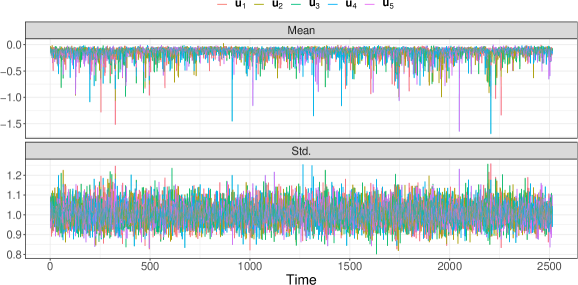
Figure 1: Posterior mean and standard deviation of $\mathbf{u}_{s},\;s=1,\dots,5$, for the inverse Wishart model (14-16) under Laplace transport map with $K=0$. The results are for a single representative simulation replica with 1000 sampling iterations.

The data set of $D=2,514$ observations of daily realized covariance matrices of $r=5$ stocks (American Express, Citigroup, General Electric, Home Depot, and IBM) spanning Jan. 1st, 2000 to Dec. 31, 2009 is described in detail in Golosnoy2012. The same model and data set was considered in grothe2017, where Gibbs sampling procedures were considered. From grothe2017, it is seen that even with close to iid sampling from $p(\mathbf{x}_{1:r}|\boldsymbol{\theta},Y_{1:D})$, the chains for $\nu$ and $\sigma_{s},\;s=1,\dots,r$ mix rather poorly under Gibbs sampling.

The ESSes for the parameters and the first elements of $\mathbf{x}_{s}$ and $\mathbf{u}_{s}$, and CPU times for Stan-Prior and Stan-Laplace are given in Table 4. Corresponding posterior means and standard deviations for Stan-Laplace ($K=0$) are given in Table 5 in the supplementary material and these are very much in line with grothe2017.

From Table 4 it is seen that the proposed methodology Stan-Laplace outperforms the benchmark Stan-Prior, both in terms CPU time (the modified target is highly non-Gaussian and thus requires many integration steps) and ESS. Indeed, Stan-Laplace with $K=0$ is at least a full order of magnitude faster in terms of ESS per CPU time than Stan-Prior for the “difficult” parameters $\nu$ and $\sigma_{s},\;s=1,\dots,r$. The added per evaluation computational cost of the more accurate Laplace approximations ($K=1$ and $K=2$) is not worthwhile, and this again corroborates the finds above that only crude location- and scale information with respect to $p(\mathbf{x}_{1:r}|\boldsymbol{\theta},Y_{1:D})$ is needed. Figure 1 depicts the posterior mean and (marginal) standard deviation of each $\mathbf{u}_{s}$, for Stan-Laplace with $K=0$. It is seen that the posterior standard deviations are close to 1, which one would expect in the case of close to perfect decoupling, i.e. is indicative that any funnel effects have been removed. The posterior means, on the other hand, are somewhat off 0, which is related both to the usage of the initial guess (7) and the fact that (17) is non-Gaussian and thus cannot be exactly decoupled using a Gaussian importance density. Figures 2,3 in the supplementary material shows corresponding plots for $K=2$ and $K=10$, and it is seen that the posterior means of $\mathbf{u}_{s}$ are closer to zero, but some deviation still exact due to the non-Gaussian target.

Comparing the computational performance to the Gibbs sampler in grothe2017, it is seen that Stan-Laplace is also roughly an order of magnitude faster than a Gibbs sampler. This comparison is somewhat complicated by that grothe2017 employ parallel processing (over $s$) when sampling the latent states $\mathbf{x}_{s}$, and that the computations in grothe2017 are done in MATLAB, whereas Stan is based on compiled C++ code. In this consideration, also the fact that a model with 20 parameters and 12,570 latent variables can be fitted using a few minutes of CPU time and minimal coding efforts in Stan must be weighed against the typically time consuming and error-prone development efforts to develop Gibbs samplers tailored for any given model.

7 Discussion

The paper proposes and evaluates importance sampler-based transport map HMC for Bayesian hierarchical models. The methodology relies on using off-the-shelf importance sampling strategies for high-dimensional latent variables to construct a modified target distribution that is easily sampled using (fixed metric) HMC. Indeed, as illustrated, the proposed methodology can lead to large speedups relative to relevant benchmarks for models with high-dimensional latent variables, while still being easily implemented using e.g. Stan.

Two strategies for selecting the involved importance samplers were considered in order to assess the optimal accuracy versus computational cost-tradeoff. The main insight in this regard is that only rather crude importance densities/transport maps (e.g. Laplace or DRHMC-type) are required when these are applied in the present framework. This observation is very much to the contrary to the importance sampling literature at large, where typically very accurate importance densities are required to produce reliable approximations to marginal likelihood functions when integrating over high-dimensional latent variables.

The proposed methodology, with Laplace transport maps and few or no Newton iterations lead to similar transport maps as those used in DRHMC in the cases where DRHMC is applicable. Thus the Laplace transport map approach may, in a rather broad sense, be seen as a generalization of DRHMC to models with nonlinear structures where DRHMC is not applicable.

Finally, there is scope for future research in developing software that can encompass a large class of models, and which implements the proposed methodology in a user-friendly manner. In particular, such software should include a sparse Cholesky algorithm for more general sparsity structures so that Laplace-based transport maps for e.g. multivariate latent state dynamic models and spatial models can be considered.

Supplementary Material for “Importance Sampling-based Transport map Hamiltonian Monte Carlo for Bayesian Hierarchical Models”

Equation numbers $<$ 18 refer to the equations in the main text.

Appendix A The Lindsten2016-integrator

The the pseduo-marginal HMC (PM-HMC) algorithm of Lindsten2016 can be viewed as a standard HMC algorithm for simulating the random vector $\mathbf{q}=(\boldsymbol{\theta}^{\prime},\mathbf{u}^{\prime})^{\prime}$ from the modified target densities (3) or (4). Proceeding with representation (4), the Hamiltonian is taken to be

$$H(\boldsymbol{\theta},\mathbf{u},\mathbf{p}_{\boldsymbol{\theta}},\mathbf{p}_{\mathbf{u}})=-\log\omega_{\mathbf{\boldsymbol{\theta}}}(\mathbf{u})-\log p(\mathbf{\boldsymbol{\theta}})+\frac{1}{2}\mathbf{u}^{\prime}\mathbf{u}+\frac{1}{2}\mathbf{p}_{\boldsymbol{\theta}}^{\prime}\mathbf{M}_{\boldsymbol{\theta}}^{-1}\mathbf{p}_{\boldsymbol{\theta}}+\frac{1}{2}\mathbf{p}_{\mathbf{u}}^{\prime}\mathbf{p}_{\mathbf{u}},$$ (18)

where $\mathbf{p}_{\boldsymbol{\theta}}\in\mathbb{R}^{d}$ and $\mathbf{p}_{\mathbf{u}}\in\mathbb{R}^{D}$ are the artificial momentum variables specific to $\boldsymbol{\theta}$ and $\mathbf{u}$, respectively. Note that for this form of the extended Hamiltonian the mass matrix ($\mathbf{M}$) of the compound vector $(\boldsymbol{\theta}^{\prime},\mathbf{u}^{\prime})^{\prime}$ is selected to be block diagonal, where the mass matrix specific to $\boldsymbol{\theta}$ is denoted by $\mathbf{M}_{\boldsymbol{\theta}}\in\mathbb{R}^{d\times d}$, while the mass for $\mathbf{u}$ is set equal to the identity in order to match the a-priori precision matrix of $\mathbf{u}$. Straight forward modifications of (18) and the proceeding theory applies if representation (3) is computationally more convenient.

Applying Hamilton’s equations (2) to the extended Hamiltonian (18), for $\mathbf{q}=(\boldsymbol{\theta}^{\prime},\mathbf{u}^{\prime})^{\prime}$ and $\mathbf{p}=(\mathbf{p}_{\boldsymbol{\theta}}^{\prime},\mathbf{p}_{\mathbf{u}}^{\prime})^{\prime}$, we get the following equations of motion

$$\frac{d}{dt}\left(\begin{array}[]{c}\boldsymbol{\theta}\\ \mathbf{p_{\boldsymbol{\theta}}}\\ \mathbf{u}\\ \mathbf{p_{u}}\end{array}\right)=\left(\begin{array}[]{c}\mathbf{M}_{\boldsymbol{\theta}}^{-1}\mathbf{p}_{\boldsymbol{\theta}}\\ \nabla_{\boldsymbol{\theta}}\log p(\boldsymbol{\theta})+\nabla_{\boldsymbol{\theta}}\log\omega_{\mathbf{\boldsymbol{\theta}}}(\mathbf{u})\\ \mathbf{p}_{\mathbf{u}}\\ -\boldsymbol{u}+\nabla_{\boldsymbol{u}}\log\omega_{\mathbf{\boldsymbol{\theta}}}(\mathbf{u})\end{array}\right).$$ (19)

Equation (19) shows that the Hamiltonian transition dynamics of $(\boldsymbol{\theta},\mathbf{p}_{\boldsymbol{\theta}})$ and $(\mathbf{u},\mathbf{p}_{\mathbf{u}})$ are linked together via their joint dependence on the importance weight $\omega_{\mathbf{\boldsymbol{\theta}}}(\mathbf{u})$. However, this link vanishes as the MC variance of the MC estimator $\text{{Var}}_{\mathbf{u}}[\omega_{\mathbf{\boldsymbol{\theta}}}(\mathbf{u})]$ tend to zero. In fact, an ‘exact’ MC estimate with zero MC variance implies that $\nabla_{\mathbf{u}}\log\omega_{\mathbf{\boldsymbol{\theta}}}(\mathbf{u})=\mathbf{0}_{D}$, in which case the transition dynamics of $(\boldsymbol{\theta},\mathbf{p}_{\boldsymbol{\theta}})$ would be completely decoupled from that of $(\mathbf{u},\mathbf{p}_{\mathbf{u}})$ and would be (marginally) the dynamics of the ‘ideal’ HMC algorithm for $p(\boldsymbol{\theta}|\mathbf{y})$. Moreover, the resulting marginal $(\mathbf{u},\mathbf{p}_{\mathbf{u}})$-dynamics would reduce to that of a harmonic oscillator with analytical solutions given by $\mathbf{u}(t)=\cos(t)\mathbf{u}(0)+\sin(t)\mathbf{p}_{\mathbf{u}}(0)$ and $\mathbf{p}_{\mathbf{u}}(t)=\cos(t)\mathbf{p}_{\mathbf{u}}(0)-\sin(t)\mathbf{u}(0)$.

In order to approximate the Hamiltonian transition dynamics (19), Lindsten2016 develop a symplectic integrator which for exact likelihood estimates produces exact simulations for the dynamics of $(\mathbf{u},\mathbf{p}_{\mathbf{u}})$ and reduces for $(\boldsymbol{\theta},\mathbf{p}_{\boldsymbol{\theta}})$ to the conventional leapfrog integrator. They derive this integrator for the special case where the mass matrix $\mathbf{M}_{\boldsymbol{\theta}}$, in (18) and (19) is restricted to be the identity. For the more general case with an unrestricted $\mathbf{M}_{\boldsymbol{\theta}}$ this integrator for approximately advancing the dynamics from time $t=0$ to time $t=\varepsilon$ is given by

$$\boldsymbol{\theta}(\varepsilon/2) =\boldsymbol{\theta}(0)+(\varepsilon/2)\mathbf{M}_{\boldsymbol{\theta}}^{-1}\mathbf{p}_{\boldsymbol{\theta}}(0),$$ (20)

$$\mathbf{u}(\varepsilon/2) =\cos(\varepsilon/2)\mathbf{u}(0)+\sin(\varepsilon/2)\mathbf{p}_{\mathbf{u}}(0),$$ (21)

$$\mathbf{p}_{\mathbf{u}}^{*} =\cos(\varepsilon/2)\mathbf{p}_{\mathbf{u}}(0)-\sin(\varepsilon/2)\mathbf{u}(0),$$ (22)

$$\mathbf{p}_{\mathbf{u}}^{**} =\mathbf{p}_{\mathbf{u}}^{*}+\varepsilon\,\nabla_{\mathbf{u}}\big{\{}\log\omega_{\boldsymbol{\theta}(\varepsilon/2)}(\mathbf{u}(\varepsilon/2))\big{\}},$$ (23)

$$\mathbf{p}_{\boldsymbol{\theta}}(\varepsilon) =\mathbf{p}_{\theta}(0)+\varepsilon\,\nabla_{\boldsymbol{\theta}}\big{\{}\log p\big{[}\boldsymbol{\theta}(\varepsilon/2)\big{]}+\log\omega_{\boldsymbol{\theta}(\varepsilon/2)}(\mathbf{u}(\varepsilon/2))\big{\}},$$ (24)

$$\boldsymbol{\theta}(\varepsilon) =\boldsymbol{\theta}(\varepsilon/2)+(\varepsilon/2)\mathbf{M}_{\boldsymbol{\theta}}^{-1}\mathbf{p}_{\boldsymbol{\theta}}(\varepsilon),$$ (25)

$$\mathbf{u}(\varepsilon) =\cos(\varepsilon/2)\mathbf{u}(\varepsilon/2)+\sin(\varepsilon/2)\mathbf{p}_{\mathbf{u}}^{**},$$ (26)

$$\mathbf{p}_{\mathbf{u}}(\varepsilon) =\cos(\varepsilon/2)\mathbf{p}_{\mathbf{u}}^{**}-\sin(\varepsilon/2)\mathbf{u}(\varepsilon/2).$$ (27)

Appendix B The EIS principle

In order to minimize the variance of IS estimates for the likelihood $p(\mathbf{y}|\boldsymbol{\theta})=\int p(\mathbf{y}|\mathbf{x},\boldsymbol{\theta})p(\mathbf{x}|\boldsymbol{\theta})d\mathbf{x}$ of non-Gaussian and/or nonlinear latent variable models, EIS aims at sequentially constructing an IS density which approximates, as closely as possible, the (infeasible) optimal IS density $m^{*}(\mathbf{x}|\boldsymbol{\theta})\propto p(\mathbf{y}|\mathbf{x},\boldsymbol{\theta})p(\mathbf{x}|\boldsymbol{\theta})$, which would reduce the variance of likelihood estimates to zero.

With reference to the likelihood it is assumed that the conditional data density $p(\mathbf{y}|\mathbf{x},\boldsymbol{\theta})$ and the prior for the latent variables $p(\mathbf{x}|\boldsymbol{\theta})$ under the latent variable model can be factorized as functions in $\mathbf{x}=(x_{1},\ldots,x_{D})$ into

$$p(\mathbf{y}|\mathbf{x},\boldsymbol{\theta})=\prod_{t=1}^{D}g_{t}(x_{t},\boldsymbol{\delta}),\qquad p(\mathbf{x}|\boldsymbol{\theta})=\prod_{t=1}^{D}f_{t}(x_{t}|\mathbf{x}_{(t-1)},\boldsymbol{\delta}),$$ (28)

where $\mathbf{x}_{(t)}=(x_{1},\ldots,x_{t})$ with $\mathbf{x}_{(D)}=\mathbf{x}$ and $\boldsymbol{\delta}=(\boldsymbol{\theta},\mathbf{y})$. Such factorizations can be found for a broad class of models, including dynamic non-Gaussian/nonlinear state-space models for time series, non-Gaussian/nonlinear models with a latent correlation structure for cross-sectional data as well as static hierarchical models without latent correlation for which $f_{t}(x_{t}|\mathbf{x}_{(t-1)},\boldsymbol{\delta})=f_{t}(x_{t},\boldsymbol{\delta})$. E.g., variants of EIS for univariate and multivariate linear Gaussian states subject to nonlinear measurements are given in Liesenfeld2003; Liesenfeld2006 and for more general nonlinear models in Kleppe201473; MOURA2014494. EIS implementations with more flexible IS densities such as mixture of normal distributions are found in KLEPPE2014449, Scharth2016133, grothe2017, and LiesenfeldRichard2010 use truncated normal distributions. Applications of EIS to models with non-Markovian latent variables for spatial data are provided in doi:10.1108/S0731-905320160000037009; doi:10.1002/jae.2534. In our applications we consider univariate time series models, which is why we use $t$ to index the elements in $\mathbf{x}$ and restrict $x_{t}$ in (28) to be one-dimensional.

EIS-MC estimation of likelihood functions $p(\mathbf{y}|\boldsymbol{\theta})$ associated with (28) is based upon an IS density $m$ for $\mathbf{x}$ which is decomposed conformably with the factorization in (28) into

$$m(\mathbf{x}|\mathbf{a})=\prod_{t=1}^{D}m_{t}(x_{t}|\mathbf{x}_{(t-1)},\mathbf{a}_{t}),$$ (29)

with conditional densities $m_{t}$ such that

$$m_{t}(x_{t}|\mathbf{x}_{(t-1)},\mathbf{a}_{t})=\frac{k_{t}(\mathbf{x}_{(t)},\mathbf{a}_{t})}{\chi_{t}(\mathbf{x}_{(t-1)},\mathbf{a}_{t})},\quad\chi_{t}(\mathbf{x}_{(t-1)},\mathbf{a}_{t})=\int k_{t}(\mathbf{x}_{(t)},\mathbf{a}_{t})dx_{t},$$ (30)

where ${\cal K}=\{k_{t}(\cdot,\mathbf{a}_{t}),\mathbf{a}_{t}\in{\cal A}_{t}\}$ is a preselected parametric class of density kernels indexed by auxiliary parameters $\mathbf{a}_{t}$ and with a point-wise computable integrating factor $\chi_{t}$. As required for the proposed methodology, it is assumed that the IS density (29) can be simulated by sequentially generating draws from the conditional densities  (30) using smooth deterministic functions $\gamma_{t}$ such that $x_{t}=\gamma_{t}(\mathbf{a}_{t},v_{t})$ for $t=1,\ldots,D$, where $v_{t}\sim N(0,1)$.

From (28)-(30) results the following factorized IS representation of the likelihood:

$$p(\mathbf{y}|\boldsymbol{\theta})=\int\left[\chi_{1}(\mathbf{a}_{1},\boldsymbol{\delta})\prod_{t=1}^{D}\omega_{t}(\mathbf{x}_{(t)},\mathbf{a}_{(t+1)},\boldsymbol{\delta})\right]m(\mathbf{x}|\mathbf{a})d\mathbf{x},$$ (31)

where the period-$t$ IS weight is given by

$$\omega_{t}(\mathbf{x}_{(t)},\mathbf{a}_{(t+1)},\boldsymbol{\delta})=\frac{g_{t}(x_{t},\boldsymbol{\delta})f_{t}(x_{t}|\mathbf{x}_{(t-1)},\boldsymbol{\delta})\chi_{t+1}(\mathbf{x}_{(t)},\mathbf{a}_{t+1},\boldsymbol{\delta})}{k_{t}(\mathbf{x}_{(t)},\mathbf{a}_{t})},$$ (32)

with $\chi_{D+1}(\cdot)\equiv 1$. For any given $\mathbf{a}=(\mathbf{a}_{1},\ldots,\mathbf{a}_{D})\in{\cal A}=\times_{t=1}^{D}{\cal A}_{t}$, the corresponding MC likelihood estimate is given by

$$\hat{p}(\mathbf{y}|\boldsymbol{\theta},\mathbf{u})=\omega(\mathbf{x},\mathbf{a}),\qquad\omega(\mathbf{x},\mathbf{a})=\prod_{t=1}^{D}\omega_{t}(\mathbf{x}_{(t)},\mathbf{a}_{(t+1)}),$$ (33)

where $\mathbf{x}$ is a draw simulated from the sequential IS density $m(\mathbf{x}|\mathbf{a})$ in (29) (which is obtained by transforming $\mathbf{u}$ using the sequence of smooth deterministic functions $\gamma_{t}$).

In order to minimize the MC variance of the likelihood estimate (33), EIS aims at selecting values for the auxiliary parameters $\mathbf{a}$ that minimize period-by-period the MC variance of the IS weights $\omega_{t}$ in (32) with respect to $m(\mathbf{x}|\mathbf{a})$. This requires that the kernels $k_{t}(\mathbf{x}_{(t)},\mathbf{a}_{t})$ as functions in $\mathbf{x}_{(t)}$ provide the best possible fit to the products $g_{t}(x_{t},\boldsymbol{\delta})f_{t}(x_{t}|\mathbf{x}_{(t-1)},\boldsymbol{\delta})\chi_{t+1}(\mathbf{x}_{(t)},\mathbf{a}_{t+1})$. For an approximate solution to this minimization problem under the preselected class of kernels ${\cal K}$, EIS solves the following back-recursive sequence of least squares (LS) approximation problems:

$$(\hat{c}_{t},\hat{\mathbf{a}}_{t})=\arg\min_{c_{t}\in\mathbb{R},\mathbf{a}_{t}\in{\cal A}_{t}}\sum_{i=1}^{r}\Bigg{\{} \log\left[g_{t}\big{(}x_{t}^{(i)},\boldsymbol{\delta}\big{)}\;f_{t}\big{(}x_{t}^{(i)}|\mathbf{x}_{(t-1)}^{(i)},\boldsymbol{\delta}\big{)}\;\chi_{t+1}\big{(}\mathbf{x}_{(t)}^{(i)},\hat{\mathbf{a}}_{t+1}\big{)}\right]$$ (34)

$$-c_{t}-\log k_{t}\big{(}\mathbf{x}_{(t)}^{(i)},\mathbf{a}_{t}\big{)}\Bigg{\}}^{2},\qquad t=D,D-1,\ldots,1,$$

where $c_{t}$ represents an intercept, and $\{{\mathbf{x}}^{(i)}\}_{i=1}^{r}$ denote $r$ iid draws simulated from $m(\mathbf{x}|\mathbf{a})$ itself. Thus, the EIS-optimal values for the auxiliary parameters $\hat{\mathbf{a}}$ result as a fixed-point solution to the sequence $\{\hat{\mathbf{a}}^{[0]},\hat{\mathbf{a}}^{[1]},\ldots\}$ in which $\hat{\mathbf{a}}^{[j]}$ is given by (34) under draws from $m(\mathbf{x}|\hat{\mathbf{a}}^{[j-1]})$. In order to ensure convergence to a fixed-point solution it is critical that all the $\mathbf{x}$ draws simulated for the sequence $\{\hat{\mathbf{a}}^{[j]}\}$ be generated by using the smooth deterministic functions $\gamma_{t}$ to transform a single set of $rD$ Common Random Numbers (CRNs), say $\mathbf{z}\sim N(\mathbf{0}_{rD},\mathbf{I}_{rD})$. To initialize the fixed-point iterations $j=0,\ldots,J$, the starting value $\hat{\mathbf{a}}^{[0]}$ can be found, e.g., from an analytical local approximation (such as Laplace) of the EIS targets $\ln(g_{t}f_{t}\chi_{t+1})$ in (34). Convergence of the iterations to a fixed-point solution is typically fast to the effect that a value for the number of iterations $J$ between 2 and 4 often suffices to produce a (close to) optimal solution (Richard2007). The MC-EIS likelihood estimate, for a given $\boldsymbol{\theta}$, is then calculated by substituting in  (33) the EIS-optimal value $\hat{\mathbf{a}}$ for $\mathbf{a}$. In order to highlight its dependence on $\boldsymbol{\theta}$ and $\mathbf{z}$ we shall use $\hat{\mathbf{a}}=\mathbf{a}(\boldsymbol{\theta},\mathbf{z})$ to denote the EIS-optimal value.

The selection of the parametric class ${\cal K}$ of EIS density kernels $k_{t}$ is inherently specific to the latent variable model under consideration as those kernels are meant to provide a functional approximation in $\mathbf{x}_{(t)}$ to the product $g_{t}f_{t}\chi_{t+1}$. In the applications below, we consider models with data densities $g_{t}$ which are log-concave in $x_{t}$ and Gaussian conditional densities for $x_{t}$ with a Markovian structure so that $f_{t}(x_{t}|\mathbf{x}_{(t-1)},\boldsymbol{\delta})=f_{t}(x_{t}|x_{t-1},\boldsymbol{\delta})$. This suggests selection of the $k_{t}$’s as Gaussian kernels and to exploit that such kernels are closed under multiplication in order to construct the $k_{t}$’s as the following parametric extensions of the prior densities $f_{t}$:

$$k_{t}(x_{t},x_{t-1},\mathbf{a}_{t})=f_{t}(x_{t}|x_{t-1},\boldsymbol{\delta})\xi_{t}(x_{t},\mathbf{a}_{t}),$$ (35)

where $\xi_{t}$ is a Gaussian kernel in $x_{t}$ of the form $\xi_{t}(x_{t},\mathbf{a}_{t})=\exp\{a_{1t}x_{t}+a_{2t}x_{t}^{2}\}$ with $\mathbf{a}_{t}=(a_{1t},a_{2t})$. In this case the EIS approximation problems (34) take the form of simple linear LS-problems where $\log[g_{t}(x_{t}^{(i)},\boldsymbol{\delta})$ $\chi_{t+1}(x_{t}^{(i)},\hat{\mathbf{a}}_{t+1})]$ are regressed on a constant, $x_{t}^{(i)}$ and $[x_{t}^{(i)}]^{2}$. In fact, (34) reduces to linear LS regressions for all kernels $k_{t}$ chosen within the exponential family (Richard2007), which simplifies implementation. However, it is important to note that EIS is by no means restricted to the use of IS densities from the exponential family nor to models with low-order Markovian specifications for the latent variables.

The EIS approach as outlined above differs from standard IS in that it uses IS densities whose parameters $\hat{\mathbf{a}}=\mathbf{a}(\boldsymbol{\theta},\mathbf{z})$ are (conditional on $\boldsymbol{\theta}$) random variables as they depend via the EIS fixed-point repressions (34) on the CRNs $\mathbf{z}$. This calls for specific rules for implementing EIS which ensure that the resulting MC likelihood estimates meet the qualifications needed for their use within PM-HMC. In order to ensure that the EIS likelihood estimate (33) based on the random numbers $\mathbf{u}$ is unbiased the latter need to be a set of random draws different from the CRNs $\mathbf{z}$ used to find $\hat{\mathbf{a}}$ (KLEPPE2014449). Note also that since $\hat{\mathbf{a}}$ is an implicit function of $\boldsymbol{\theta}$, maximal accuracy requires us to rerun the EIS fixed-point regressions for any new value of $\boldsymbol{\theta}$. In order to ensure that the resulting EIS likelihood estimate (33) as a function of $\hat{\mathbf{a}}$ is smooth in $\boldsymbol{\theta}$, $\hat{\mathbf{a}}$ itself needs to be a smooth function of $\boldsymbol{\theta}$. This can be achieved by presetting the number of fixed-point iterations $J$ across all $\boldsymbol{\theta}$-values to a fixed number, rather than using a stopping rule based on a relative-change threshold.

The EIS-specific tuning parameters are the number of $\mathbf{x}^{(i)}$-draws $r$ used to run the EIS optimization process, the number of fixed-point iterations on the EIS regressions $J$, and the number of $\mathbf{x}^{(i)}$-draws $n$ for the likelihood estimate (33). Those parameters should be selected to balance the trade-off between EIS computing time and the quality of the resulting EIS density with respect to the MC accuracy. In particular, for $r$ it is recommended to select it as small as possible while retaining the EIS fixed-point regressions numerically stable and the parameter $J$ should be set such that it is guaranteed that the fixed-point sequence $\{\mathbf{a}^{[j]}\}_{j}$ approximately converge for the $\boldsymbol{\theta}$ values in the relevant range of the parameter space. In our applications, where the selected class of kernels ${\cal K}$ imply that the EIS regressions are linear in the EIS parameters $\mathbf{a}_{t}$, we find that a $J$ set equal to 1 or 2 and an $r$ about 2 times the number of parameters in $(\mathbf{a}_{t},c_{t})$ suffice. We obtain EIS kernels $k_{t}$ providing highly accurate approximations to the targeted product $g_{t}f_{t}\chi_{t+1}$, with an $R^{2}$ of the EIS regressions in the final iteration typically larger than 0.95.

Appendix C Details related to the example models in Section 5

C.1 SV model

For the SV model, the standard prior assumptions for the parameters $\boldsymbol{\theta}=(\gamma,\delta,\nu)$ are the following: for $\gamma$ we use a flat prior, for $(\delta+1)/2$ a Beta prior ${\cal{B}(\alpha,\beta)}$ with $\alpha=20$ and $\beta=1.5$, and for $\nu^{2}$ a scaled inverted-$\chi^{2}$ prior $p_{0}s_{0}/\chi_{(p_{0})}^{2}$ with $p_{0}=10$ and $s_{0}=0.01$. For numerical stability we use the parametrization $\boldsymbol{\theta}^{*}=(\gamma,\mbox{arctanh}\,\delta,\log\nu^{2})$ together with the priors for $\boldsymbol{\theta}^{*}$ to run the HMC algorithms, where the priors are derived from those on $\boldsymbol{\theta}$.

For the Laplace transport map, $\mathbf{G}_{\boldsymbol{\theta}}^{(0)}$ and $\mathbf{h}_{\boldsymbol{\theta}}^{(0)}$ are taken to be identical to (6,7). More refined solutions are found using Newton iterations;

$$\mathbf{h}_{\boldsymbol{\theta}}^{(k)} =\mathbf{h}_{\boldsymbol{\theta}}^{(k-1)}+\left[\nabla_{\mathbf{x}}^{2}\log\left[p(\mathbf{x}|\boldsymbol{\theta})p(\mathbf{y}|\mathbf{x},\boldsymbol{\theta})\right]_{\mathbf{x}=\mathbf{h}_{\boldsymbol{\theta}}^{(k-1)}}\right]^{-1}\left\{\nabla_{\mathbf{x}}\log\left[p(\mathbf{x}|\boldsymbol{\theta})p(\mathbf{y}|\mathbf{x},\boldsymbol{\theta})\right]_{\mathbf{x}=\mathbf{h}_{\boldsymbol{\theta}}^{(k-1)}}\right\},$$

$$\mathbf{G}_{\boldsymbol{\theta}}^{(k)} =\nabla_{\mathbf{x}}^{2}\log\left[p(\mathbf{x}|\boldsymbol{\theta})p(\mathbf{y}|\mathbf{x},\boldsymbol{\theta})\right]_{\mathbf{x}=\mathbf{h}_{\boldsymbol{\theta}}^{(k-1)}}.$$

for $k=1,2,\dots,K$. Further modifications, including changing to $\mathbf{G}_{\boldsymbol{\theta}}^{(k)}=\nabla_{\mathbf{x}}^{2}\log\left[p(\mathbf{x}|\boldsymbol{\theta})p(\mathbf{y}|\mathbf{x},\boldsymbol{\theta})\right]_{\mathbf{x}=\mathbf{h}_{\boldsymbol{\theta}}^{(k)}}$ (at the cost of one additional Cholesky factorization), or keeping $\mathbf{G}_{\boldsymbol{\theta}}^{(k)}=\mathbf{G}_{\boldsymbol{\theta}}^{(0)}$ (costs only a single Cholesky factorization) both in the transport map and as the scaling matrix in the Newton iterations was tried, but did not produce better results.

It is straight forward to show that $\mathbf{G}_{\boldsymbol{\theta},\mathbf{y}|\mathbf{x}}=0.5\mathbf{I}_{D}$ is also the Fisher information of $p(\mathbf{y}|\mathbf{x})$ with respect to $\mathbf{x}$ (i.e. $p(\mathbf{y}|\mathbf{x})$ is a constant information parameterization). Hence also Stan-Laplace $K=0$ may be interpreted as a special case of DRHMC (1806.02068).

C.2 Gamma model

For the Gamma model, the priors on the parameters $\boldsymbol{\theta}=(\tau,\beta,\delta,\nu)$ are as follows; we use flat priors for $\log\tau$ as well as $\log\beta$, a Beta ${\cal{B}(\alpha,\beta)}$ with $\alpha=20$ and $\beta=1.5$ for $(\delta+1)/2$, and a scaled inverted-$\chi^{2}$ for $\nu^{2}$ with $p_{0}s_{0}/\chi_{(p_{0})}^{2}$ and $p_{0}=10$, $s_{0}=0.01$. For the LD computations we use the parameterization $\boldsymbol{\theta}^{*}=(\log\tau,\log\beta,\mbox{arctanh}\,\delta,\log\nu^{2})$.

For this model, the same strategy for calculating the Laplace transport map as for the SV model was used. Notice that here $\mathbf{G}_{\boldsymbol{\theta},\mathbf{y}|\mathbf{x}}=\tau^{-1}\mathbf{I}_{D}$ is also the Fisher information of $p(\mathbf{y}|\mathbf{x})$ with respect to $\mathbf{x}$. Hence, Stan-Laplace, $K=0$ may be interpreted as a DRHMC method.

C.3 CEV model

For the CEV model, for $\alpha$ and $\beta$ we assume Gaussian priors both with $N(0,1000)$, for $\gamma$ a uniform prior on the interval $[0,4]$, and for $\sigma_{x}^{2}$ and $\sigma_{y}^{2}$ uninformative inverted-$\chi^{2}$ priors with $p(\sigma_{x}^{2})\propto 1/\sigma_{x}^{2}$ and $p(\sigma_{y}^{2})\propto 1/\sigma_{y}^{2}$. The LD computations are conducted on the following transformed parameters: $\boldsymbol{\theta}^{*}=(\alpha,\beta,\gamma,\log{\sigma_{x}^{2}},\log{\sigma_{y}^{2}})$.

For the CEV model, the precision of the latent state prior is does not have closed-form, which precludes the application of (6,7). However, it is known that the measurement densities has a very small variance, hence $\mathbf{h}_{\boldsymbol{\theta}}^{(0)}=\mathbf{y}$ seems sensible. Subsequently, a full Newton iteration is performed:

$$\mathbf{h}_{\boldsymbol{\theta}}^{(k)} =\mathbf{h}_{\boldsymbol{\theta}}^{(k-1)}+\left[\nabla_{\mathbf{x}}^{2}\log\left[p(\mathbf{x}|\boldsymbol{\theta})p(\mathbf{y}|\mathbf{x},\boldsymbol{\theta})\right]_{\mathbf{x}=\mathbf{h}_{\boldsymbol{\theta}}^{(k-1)}}\right]^{-1}\left\{\nabla_{\mathbf{x}}\log\left[p(\mathbf{x}|\boldsymbol{\theta})p(\mathbf{y}|\mathbf{x},\boldsymbol{\theta})\right]_{\mathbf{x}=\mathbf{h}_{\boldsymbol{\theta}}^{(k-1)}}\right\},$$

$$\mathbf{G}_{\boldsymbol{\theta}}^{(k)} =\nabla_{\mathbf{x}}^{2}\log\left[p(\mathbf{x}|\boldsymbol{\theta})p(\mathbf{y}|\mathbf{x},\boldsymbol{\theta})\right]_{\mathbf{x}=\mathbf{h}_{\boldsymbol{\theta}}^{(k-1)}}.$$

for $k=1,2,\dots,K$. Further modifications, including changing to $\mathbf{G}_{\boldsymbol{\theta}}^{(k)}=\nabla_{\mathbf{x}}^{2}\log\left[p(\mathbf{x}|\boldsymbol{\theta})p(\mathbf{y}|\mathbf{x},\boldsymbol{\theta})\right]_{\mathbf{x}=\mathbf{h}_{\boldsymbol{\theta}}^{(k)}}$ (at the cost of one additional Cholesky factorization) did not improve the fit sufficiently to warrant the additional computation.

Appendix D Details related to the realized volatility model in Section 6

	$\mu_{1}$	$\mu_{2}$	$\mu_{3}$	$\mu_{4}$	$\mu_{5}$	$\delta_{1}$	$\delta_{2}$	$\delta_{3}$	$\delta_{4}$	$\delta_{5}$
post. mean	4.16	4.12	3.72	4.11	3.53	0.97	0.98	0.96	0.94	0.96
post. std.	0.2	0.25	0.15	0.1	0.13	0.005	0.004	0.006	0.008	0.006
	$\sigma_{1}$	$\sigma_{2}$	$\sigma_{3}$	$\sigma_{4}$	$\sigma_{5}$	$\nu$
post. mean	0.31	0.26	0.29	0.28	0.25	33.61
post. std.	0.009	0.008	0.009	0.009	0.009	0.283
	$h_{2,1}$	$h_{3,1}$	$h_{4,1}$	$h_{5,1}$	$h_{3,2}$	$h_{4,2}$	$h_{5,2}$	$h_{4,3}$	$h_{5,3}$	$h_{5,4}$
post. mean	0.39	0.29	0.29	0.23	0.20	0.17	0.12	0.22	0.18	0.11
post. std.	0.003	0.003	0.003	0.002	0.003	0.003	0.002	0.004	0.003	0.002
	$x_{1,1}$	$x_{2,1}$	$x_{3,1}$	$x_{4,1}$	$x_{5,1}$	$u_{1,1}$	$u_{2,1}$	$u_{3,1}$	$u_{4,1}$	$u_{5,1}$
post. mean	5.23	5.28	4.27	5.46	5.11	-0.08	-0.05	-0.07	-0.10	-0.10
post. std.	0.206	0.195	0.198	0.205	0.202	1.022	0.993	0.99	1.031	1.049

Table 5: Posterior mean and standard deviations for the inverse Wishart model (14-16) based on Stan-Laplace, $K=0$. All figures are means across 8 independent replica. Here, $u_{s,1}$ is the first element in $\mathbf{u}_{s}$, and should be close to standard normal when the transport map produces a sufficient de-coupling effect.

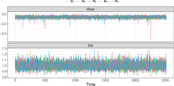
Figure 2: Posterior mean and standard deviation of $\mathbf{u}_{s},\;s=1,\dots,5$, for the inverse Wishart model (14-16) under Laplace transport map with $K=2$.

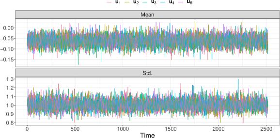
Figure 3: Posterior mean and standard deviation of $\mathbf{u}_{s},\;s=1,\dots,5$, for the inverse Wishart model (14-16) under Laplace transport with $K=10$.

The (normalized) observation density is given by:

$$p(\mathbf{Y}_{t}|\Sigma_{t},\nu)=\frac{|\boldsymbol{\Sigma}_{t}|^{\frac{\nu}{2}}}{2^{\frac{\nu r}{2}}\pi^{\frac{r(r-1)}{4}}\prod_{s=1}^{r}\Gamma\left([\nu+1-s]/2\right)}|\mathbf{Y}_{t}|^{-\frac{\nu+r+1}{2}}\exp\left(-\frac{1}{2}\text{tr}\left[\boldsymbol{\Sigma}_{t}\mathbf{Y}_{t}^{-1}\right]\right).$$

In the Stan implementation, $\prod_{t=1}^{D}|\mathbf{Y}_{t}|$ and $\mathbf{Y}_{t}^{-1},\;t=1,\dots,D$ where precomputed.

The (independent) priors used to complete the model specification in Section 6.1 are as follows: $\mu_{s}\sim N(0,25)$, $\delta_{s}\sim\text{uniform}(-1,1)$, $\sigma_{s}^{2}\sim p_{0}s_{0}/\chi_{p_{0}}^{2}$ where $p_{0}=4$ and $s_{0}=0.25$, $h_{i,j}\sim N(0,100)$. Finally, a flat prior on $(6.0,\infty)$ was chosen for $\nu$.

Posterior- means and standard deviations of the parameters and the first elements in $\mathbf{x}_{s}$ and $\mathbf{u}_{s}$ are given in Table 5. The results are very much in line with those of grothe2017.

The Laplace transport maps for each of $\mathbf{x}_{s},\;s=1,\dots,r$ are constructed as follows; the initial guesses for $\mathbf{h}_{\boldsymbol{\theta}}^{(0)}$ and $\mathbf{G}_{\boldsymbol{\theta}}^{(0)}$ are those given in (6,7), applied to (17). The mean is further refined via the following approximate Newton iteration

$$\mathbf{h}_{\boldsymbol{\theta}}^{(k)}=\mathbf{h}_{\boldsymbol{\theta}}^{(k-1)}+\left[\mathbf{G}_{\boldsymbol{\theta}}^{(0)}\right]^{-1}\left\{\nabla_{\mathbf{x}}\log\left[p(\mathbf{x}|\boldsymbol{\theta})p(\mathbf{y}|\mathbf{x},\boldsymbol{\theta})\right]_{\mathbf{x}=\mathbf{h}_{\boldsymbol{\theta}}^{(k-1)}}\right\},$$

whereas $\mathbf{G}_{\boldsymbol{\theta}}^{(k)}=\mathbf{G}_{\boldsymbol{\theta}}^{(0)}$ is kept fixed which result in that only a single Cholesky factorization is required. Figures 2,3 show the posterior mean and standard deviations of $\mathbf{u}_{s}$ over time $t$ for Stan-Laplace, $K=2$ and $K=10$ respectively. It is seen that even with the approximate Newton iteration, the iteration makes $\mathbf{u}_{s}$ have a mean close to zero, where the remaining deviation from zero for $K=10$ iterations in Figure 3 is presumably due to the non-quadratic nature of the "measurement density" in (17) (in addition to Monte Carlo variation).