An Empirical Evaluation of Sketched SVD and its Application to Leverage Score Ordering

Abstract

The power of randomized algorithms in numerical methods have led to fast solutions which use the Singular Value Decomposition (SVD) as a core routine. However, given the large data size of modern and the modest runtime of SVD, most practical algorithms would require some form of approximation, such as sketching, when running SVD. While these approximation methods satisfy many theoretical guarantees, we provide the first algorithmic implementations for sketch-and-solve SVD problems on real-world, large-scale datasets. We provide a comprehensive empirical evaluation of these algorithms and provide guidelines on how to ensure accurate deployment to real-world data. As an application of sketched SVD, we present Sketched Leverage Score Ordering, a technique for determining the ordering of data in the training of neural networks. Our technique is based on the distributed computation of leverage scores using random projections. These computed leverage scores provide a flexible and efficient method to determine the optimal ordering of training data without manual intervention or annotations. We present empirical results on an extensive set of experiments across image classification, language sentiment analysis, and multi-modal sentiment analysis. Our method is faster compared to standard randomized projection algorithms and shows improvements in convergence and results.

1 Introduction

Many problems in numerical methods rely heavily on the Singular Value Decomposition (SVD), a technique for factorizing a real or complex matrix. Such problems include low-rank approximations, computation of leverage scores, pseudo-inverses, and including their weighted and robust variants. These applications have become more important with the advent of big data and large-scale machine learning. For example, weighted low rank approximations are used in recommendation systems (Razenshteyn et al., 2016; Markovsky, 2008) and leverage scores are heavily used in statistical data analysis (Wei et al., 1998; Drineas et al., 2011). While the exact computation of the SVD can provide deterministic solutions to these problems, these algorithms are often too slow on large-scale datasets. As a result, research has focused on efficient approximate algorithms for scalable computation of the SVD.

Recently, the power of randomized algorithms has led to much faster solutions to these problems. These randomized algorithms for numerical linear algebra were popularized by the sketching method (Woodruff, 2014). The basis for these sketching algorithms involves multiplying the data matrix $\mathbf{X}\in\mathbb{R}^{n\times d}$ with a smaller randomized matrix. The sketched problem is then smaller and can be solved using the same algorithm in faster input runtime. Although the truncated SVD (Hansen, 1987) and other iterative SVD algorithms (Cho and Reyhani, 2012) also provide efficient alternatives, sketching algorithms are more efficient and accurate, especially when the input is sparse (Woodruff, 2014).

While these sketching methods satisfy theoretical guarantees (Drineas et al., 2011; Woodruff, 2014) (see details in section 2), our contribution lies in the first implementations of these algorithms for sketching SVD problems on real-world, large-scale datasets. We found that the naive implementation of sketched SVD leads to several problems such as difficulties in estimating true ranks of real-world datasets, corruption by high-dimensional noise, and impact of small singular values. We provide a comprehensive empirical evaluation of these algorithms and summarize guidelines on how to ensure accurate deployment to real-world data. Finally, we examine an application of sketched SVD on the efficient computation of leverage scores. We apply the sketched leverage scores as an ordering method for curriculum learning, and show improved performance over random ordering when training deep neural networks on three datasets. Although (Dahiya et al., 2018) also empirically evaluate sketching, they focus on general algorithms rather than a treatment of SVD problems. We further provide an application of sketched SVD for curriculum learning.

The remainder of the paper is organized as follows. We first state several preliminary results in section 2. We then provide valuable insights into the practical implementations of sketched SVD on large-scale datasets in section 3. In section 4 we outline the application of sketched SVD: the Sketched Leverage Score Ordering algorithm. We present experimental results in section 5. We then discuss our observations in section 6. Finally, we describe related work and conclude the paper in sections 7 and 8 respectively.

2 Preliminaries

2.1 Sketching and Subspace Embeddings

Popular choices for the randomized sketching matrix include random Gaussian matrices (Woodruff, 2014), the Fast Johnson Lindenstrauss transform (FJLT) (Sarlos, 2006), the Subsampled Randomized Hadamard Transform (SRHT) (Boutsidis and Gittens, 2012; Tropp, 2011), the CountSketch matrix (Bourgain et al., 2015; Clarkson and Woodruff, 2017; Cohen, 2016; Meng and Mahoney, 2013) or the OSNAP matrix (Nelson and Nguyên, 2013). All these sketching matrix $\mathbf{S}$ are useful because they satisfy the subspace embedding property:

Definition 2.1.

Subspace Embedding: Let $\mathbf{A}$ be a $n$ by $d$ matrix. A $(1\pm\epsilon)$ $\ell$2 subspace embedding for the column space of $\mathbf{A}$ is a k by n matrix $\mathbf{S}$ such that $\forall x\in\mathbb{R}^{n}$,

$$(1-\epsilon)\|\mathbf{A}x\|^{2}_{2}\leq\|\mathbf{SA}x\|^{2}_{2}\leq(1+\epsilon)\|\mathbf{A}x\|^{2}_{2}$$

Theorem 2.2.

A subspace embedding preserves the set of singular values, of the input matrix $\mathbf{A}$. In particular, if $\mathbf{S}$ is a $(1\pm\epsilon)$ $\ell$2 subspace embedding for $\mathbf{A}$, then:

$$\sigma_{k}(\mathbf{SA})=(1\pm O(\epsilon))\sigma_{k}(\mathbf{A})$$

A proof of theorem 2.2 is given in (Li et al., 2014). In addition to least squares regression, L1 regression, and low-rank approximations (Woodruff, 2014), more recent applications of sketching also include low-rank tensor regression (Haupt et al., 2017), $q$ to $p$ norms (Krishnan et al., 2018), and Kronecker product regression (Diao et al., 2018).

2.2 Leverage Scores Sampling

The subspace embedding methods presented above are oblivious to the structure of the input matrix $\mathbf{A}$. For example if a CountSketch matrix $\mathbf{S}$ is used to embed $\mathbf{A}$ and $\mathbf{A}$ has sparse rows, then $\mathbf{SA}$ has sparse rows too. However, there are applications in which the goal is to sample the important rows thus having a sparse $\mathbf{SA}$ is not helpful.

The leverage score of a data point is a measure of how much an outlier the data point is from other points in data $\mathbf{A}$. The underlying data model is assumed to be linear and the leverage score of the $i$th point, $l_{i}$, is given by $i$th row norm of the projection matrix of $\mathbf{A}$, i.e

$$l_{i}=|[\mathbf{H}]_{i}|^{2}_{2},\;\mathbf{H}=\mathbf{A}(\mathbf{A}^{T}\mathbf{A})^{+}\mathbf{A}^{T}$$

Alternatively, taking the Singular Value Decomposition, $\mathbf{A}=\mathbf{U\Sigma V}^{T}$, $l_{i}$ can be expressed as

$$l_{i}=|\mathbf{U}_{i,*}|^{2}_{2}$$

Computing the leverage scores naively requires a costly matrix inversion, which can be prohibitive for very large data sets. Fortunately, the techniques of matrix sketching can be used to approximate the leverage scores (Drineas et al., 2011).

3 Practical Implementation of Fast Leverage Scores

(Drineas et al., 2011) showed that sketching produces a small but good subspace embedding for finding the orthonormal basis. In the sketch space, the orthonormal basis can then computed using a Singular Value Decomposition (SVD). Also, (Drineas et al., 2011) gave the procedures of finding 1) exact leverage scores by SVD and 2) an $(1+\epsilon)$ approximation to the leverage scores by sketching:

Algorithm 1 Exact Leverage Score by SVD

Input :

Given $n\times d$ matrix $\mathbf{A}$.

Output :

Leverage score of $i$th row as $l_{i}$.

1. Compute SVD, $\mathbf{A}=\mathbf{U\Sigma V}^{T}$.

2. Compute $l_{i}$ from the first $d$ columns of the $i$th row $l_{i}=|\mathbf{U}_{i}|^{2}_{2}$.

Algorithm 2 Approximation Leverage Score by Sketching

Input :

Given $n\times d$ matrix $\mathbf{A}$.

Output :

Approximate Leverage score of $i$th row as $l_{i}$.

1. Compute Sketch of $\mathbf{A}$, $\mathbf{SA}$.

2. Compute SVD, $\mathbf{SA}=\mathbf{U\Sigma V}^{T}$.

3. Compute $\mathbf{U}^{approx}=\mathbf{AV}^{T}\mathbf{\Sigma}^{-1}$.

4. Compute $l_{i}$ from the first $D$ columns of the $i$th row $l_{i}=|\mathbf{U}^{approx}_{i}|^{2}_{2}$.

3.1 Implementation Details

The following sketching schemes were implemented in Python 3.6 and tested for their performance on a 64-bit machines with i7 CPU with 12 cores and 32 GB RAM.

3.1.1 SVD for Exact Leverage Scores

The SVD used for the exact computation of leverage scores (Algorithm 1) is from numpy.linalg.svd which uses LAPACK’s SVD routines. It is highly optimized and multithreaded, take advantaging of the multi-cores CPU.

3.1.2 Approximate Leverage Scores

To compute approximate leverage scores via sketching (Algorithm 2), we examine the following choices for sketching matrices $\mathbf{S}$:

Subsampled Randomized Hadamard Transform: A Fast Johnson Lindenstrauss sketching matrix was implemented as a Subsampled Randomized Hadamard Transform (SRHT). The core Hadamard Transform was implemented using the Faster Fast Hadamard Transform (FFHT) of (Andoni et al., 2015) and uses Advanced Vector Extensions (AVX) CPU instructions to speed up the Hadamard Transform. Below is a synthetic data test run for comparing SVD vs SRHT to compute leverage scores (Table 1). However, we decided to drop SRHT from future experiments as it is difficult to meet the SRHT unique requirement of the row having to be a power of 2.

Data size = $n\times$ 50	Running Time in Seconds
$n=$	$2^{16}$	$2^{18}$	$2^{20}$	$2^{22}$	$2^{24}$
Sketching	0.9	3.3	5.4	13.5	122.5
SVD	0.7	3.3	13.9	57.2	2114.0

Table 1: Running time for Synthetic Data. Sketching’s $\epsilon=0.25$. Sketching matrices indeed increase running time significantly when $n$ increases.

CountSketch, OSNAP: OSNAP is a variant of CountSketch as described in (Nelson and Nguyên, 2013). Both CountSketch and OSNAP are implemented in Python using the Numpy Library without additional acceleration. They are implemented in the streaming model where the sketching matrix rows are updated as the rows of the original matrix are read. Both sketches are implemented as a pair of hash functions.

3.1.3 Distributed Sketch, Coordinator Model

We implemented the distributed sketching, coordinator model framework for CountSketch and OSNAP as described in (Balcan et al., 2015). The simulation of a distributed computing network was done using multiple processes using the Multiprocessing library in python. To simulate a row partition model, the data was fed to each process before sketching was completed. A single process acted as the coordinator. In this setup, there is minimal overhead penalty for the communication cost.

3.2 Implementation Experiments for Timing Performance

The following experiments were meant to compare the performance of approximate leverage scores under different matrices. The number of rows for each sketching matrix was determined using their theoretical guarantees: $O((d/\epsilon)^{2})$ for CountSketch and $O(d/\epsilon^{2}\log d)$ for OSNAP. For all experiments, the timings shown are for the actual time taken to compute the leverage scores. This excludes the time for data generation, setup and the output of the final scores.

Synthetic Data, Skinny Matrix: Table 2 shows that CountSketch is competitive when the number of column dimensions are small.

K	SVD	CountSketch	OSNAP
10	0.001	0.22	0.22
14	0.009	0.23	0.63
18	0.21	0.73	5.12
22	3.76	0.11	73.5

Table 2: $N=2^{k},D=16$, 8 Threads, Sketching’s $\epsilon=0.5$, Timings in seconds.

Synthetic Data: Table 3 shows that sketching is faster than SVD as the matrices increase in size.

K	SVD	CountSketch	OSNAP
10	0.06	0.28	0.29
14	0.41	1.02	0.98
18	10.26	16.44	12.15
22	257.55	45.16	169.44

Table 3: $N=2^{k},D=256$, 8 Threads, Sketching’s $\epsilon=0.5$, Timings in seconds.

Synthetic Data, Squarish Matrix: Table 4 shows that OSNAP sketching is slightly faster than SVD for large matrices in both rows and columns. CountSketch was not used as it does not meet the requirements on the number of rows.

K	SVD	OSNAP
16	192.43	155.53

Table 4: $N=2^{16},D=2^{12}$ 8 Threads, Sketching’s $\epsilon=0.5$, Timings in seconds.

3.3 Implementation Experiments on the Effects of Column Rank on Leverage Scores Approximation

An assumption in most of the bounds for sketching matrices for subspace embedding is that the matrix $A$ has full column rank (Drineas et al., 2011; Clarkson and Woodruff, 2017). However this is not a realistic assumption for most real world data as the latent dimension of the data might not be known. Real world data is often generated from a low dimensional subspace and corrupted with high dimensional noise. The following experiments test the effects of getting a wrong estimate for the column rank of the matrix that sketching is applied on. The two sketching matrices tested were CountSketch and SRHT. OSNAP was not tested as it can be seen as a variant of CountSketch.

Figure 1: Plot of sketched (Countsketch, FJLT) vs actual leverage scores when the data matrix has full column rank. Approximate leverage scores are close to the actual scores.

Figure 2: Plot of sketched (Countsketch, FJLT) vs actual leverage scores when the data matrix has column rank half of column dimension. When the column rank is wrong, even by a factor of 2, the approximate leverage scores computed can be significantly off.

From Figures 1 and 2, we observe that when the column rank is the same as the dimension, then as suggested by the theoretical bounds, the quality of the approximated leverage scores is a function of the approximation factor $\epsilon$. However, when the column rank is wrong, even by a factor of 2, then the approximate leverage scores computed can be significantly off and the approximation error can be unbounded.

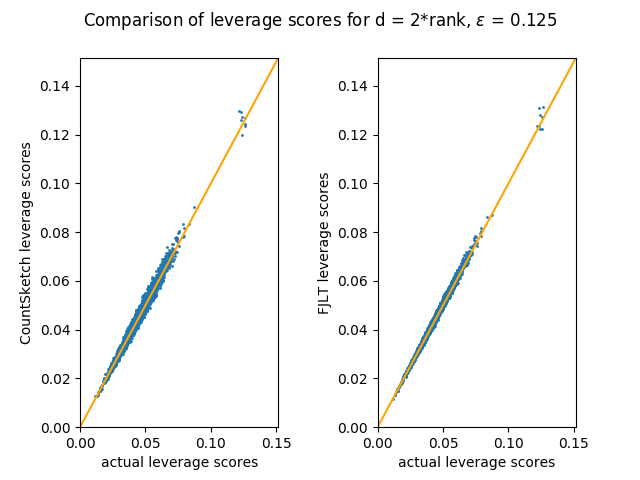
Figure 3: Plot of sketched (Countsketch, FJLT) vs actual leverage scores when the column orthonormal basis that is computed from the sketched matrix is truncated to the true rank of the original data. Approximate leverage scores are now close to the actual scores, as desired.

However, if the column orthonormal basis that is computed from the sketched matrix is truncated to the true rank of the original data, the approximate leverage score is a function of the approximation factor $\epsilon$ (Figure 3). Both experiments show that having the column rank meeting the column dimension is a hard requirement, failing which would result in an unbounded approximation error.

3.4 Effects of Small Singular Values on Leverage Scores Approximation

When the data is corrupted by small amount of high rank noise, it would appear as though it has full column rank. An example of high rank noise would be additive Gaussian white noise. For example, shown in Figure 4 is a plot of the singular values of the MNIST handwriting training data, where each training example is flattened into a row vector and the entire data set is stacked vertically to form a $60000\times 764$ matrix.

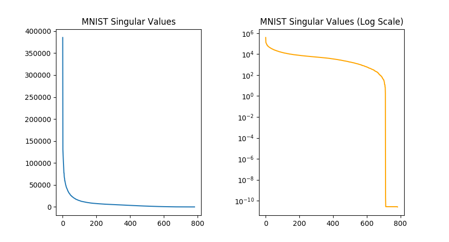
Figure 4: Singular values of the MNIST dataset, on original (left) and log (right) scale.

After applying the approximation leverage score described so far, we can see from Figure 5 (left) that the approximation error can be much larger than the $\epsilon$ factor used and it looks similar to the case where the column rank was less than the column dimension. The error can be attributed to numerical precision errors when very small singulars are inverted to compute the orthonormal basis from the sketch. i.e step 3, $\mathbf{U}^{\text{approx}}=\mathbf{AV}^{T}\mathbf{\Sigma}^{-1}$.

3.5 Modified Leverage Scores Approximation by Sketching

Algorithm 3 Approximate Leverage Score with Truncation

Input :

Given $n\times d$ matrix $\mathbf{A}$, threshold $\epsilon$.

Output :

Approximate Leverage score of $i$th row as $l_{i}$.

1. Compute Sketch of $\mathbf{A}$, $\mathbf{SA}$.

2. Compute SVD, $\mathbf{SA=U\Sigma V}^{T}$.

3. Truncate $\mathbf{V},\mathbf{\Sigma}$ at small singular values less than $\epsilon$. Let this truncated matrices be $\mathbf{V}^{\prime}$, $\mathbf{\Sigma^{\prime}}$

4. Compute $\mathbf{U}^{approx}=\mathbf{AV^{\prime}}^{T}\mathbf{\Sigma^{\prime}}^{-1}$.

5. Compute $l_{i}$ from the first $d$ columns of the $i$th row $l_{i}=|\mathbf{U}^{approx}_{i}|^{2}_{2}$.

Small singular values would appear in the sketched matrix $\mathbf{SA}$ since the sketching matrix is a subspace embedding of $\mathbf{A}$. To see this, consider the smallest non-zero eigenvalue, $\lambda_{1}$:

$$\mathbf{A}v =\lambda_{1}v$$

$$|\mathbf{SA}v| =(1+\epsilon)|\mathbf{A}v|_{2}$$

$$=(1+\epsilon)\lambda_{1}$$

This agrees with the experimental results on the MNIST dataset. With the modified leverage score approximation algorithm, we recover the leverage scores to the approximation factor as guaranteed, from Figure 5 (right). Using these insights, we summarize the following modifications to the Approximate Leverage Score algorithm, in Algorithm 3.

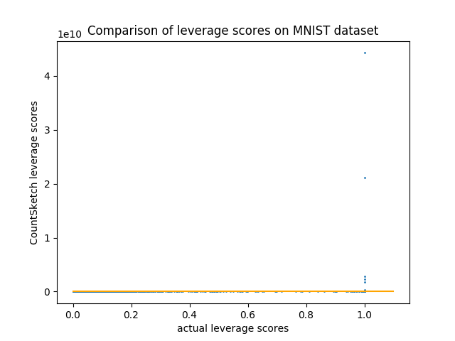
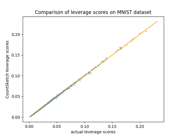
Figure 5: Sketched leverage scores in comparison with actual leverage scores. Left: without truncation, right: after truncation for smallest singular values, giving the desired accuracies.

3.6 Practical Implementation Remarks

We tested different implementations of sketched leverage scores to compare theoretical guarantees and practical performance. The sketches tested included Subsampled Randomized Hadamard Transform, CountSketch and OSNAP. In addition, sketching for CountSketch and OSNAP was implemented in a distributed setting using the central coordinator model.

We found that the SRHT requirement of having rows as a power of 2 was impractical. The memory and timing overheads required to satisfy that requirement is prohibitive. OSNAP is more useful for real world data as it requires less rows. Most curated datasets do not have enough rows ($n$) so that CountSketch requirements can be satisfied.

Figure 6: Popular image datasets for deep learning tasks. All of these datasets do not satisfy the $n\geq 4d^{2}$ requirement for CountSketch. The situation is worse when temporal data (i.e. text, videos, time series) is concerned since $d$ grows in both the feature and temporal dimensions.

We found that the quality of the sketch is highly dependent on the column rank of the data. If the column rank of the data is less than the column dimension, then the approximation error can be unbounded. Requiring a full rank matrix for sketching as described in (Clarkson and Woodruff, 2017) is a hard requirement.

Lastly, we found that small singular values in real data can corrupt the approximate leverage scores returned by sketching. This happens often as real data have high rank noise. We proposed a new algorithm to compute approximate leverage scores by first truncating the singular values before computing an approximate orthonormal basis. Experimentally, this modification recovers the approximate leverage scores to within the approximation guarantees given by sketching.

4 Sketched Leverage Score Ordering

In this section, we describe an application of sketched leverage scores for training deep neural networks. The optimization of deep neural networks is largely based on stochastic gradient methods. Given the immense applications of deep neural networks, the empirical convergence and training speed of these networks and stochastic gradient methods have become important research areas.

We focus on curriculum learning, a research area which aims to determine optimal orderings of training data to improve convergence and performance of neural networks (Bengio et al., 2009). Curriculum Learning has traditionally focused on either manually determining a training order (Bengio et al., 2009; Spitkovsky et al., 2010; Khan et al., 2011) or using auxiliary networks to jointly optimize for the optimal training order (Kumar et al., 2010; Jiang et al., 2015). However, neither manual annotations nor costly overhead training times are ideal for training large neural networks on huge datasets.

Algorithm 4 Sketched Leverage Score Ordering

Input :

Given $n$ data points each with $d$ features

1. Stack data points to form a $n\times d$ matrix $\mathbf{A}$

2. Compute leverage scores, $L=$ApproxLeverageScoreWithTruncation($\mathbf{A}$)

3. Form the sampling probability $P_{i}$ for each data point from the leverage scores, $P=L_{i}/\Sigma_{i}L_{i}$

for each training epoch do

       4. Order the data points using sampling policy $\pi$ on distribution $P$. 5. Send the mini-batches for training in the given order.

end for

To address the shortcomings in Curriculum Learning, we present Sketched Leverage Score Ordering (SLSO), a novel technique for determining the ordering of data in the training of neural networks. SLSO does not rely on manual annotations and is faster than policy gradient sampling methods in training auxiliary networks.

SLSO is shown in Algorithm 4 and is based on approximating the leverage scores using matrix sketching techniques, so as to cater to the size of large datasets. These computed leverage scores provide a flexible and efficient method to determine the optimal ordering of training data without manual intervention or annotations. In particular, leverage scores can be used to estimate the importance of a training example. Larger leverage scores correspond to training examples that are more important. The sampling policy $\pi$ allows flexible design of the curriculum: leverage scores can be used independently or combined with an existing curriculum based on prior knowledge of the task. Furthermore, the leverage scores can be computed on either raw features or from semantic latent spaces using a pretrained network.

5 Experiments

5.1 Datasets

We perform extensive evaluations across 3 datasets from 3 different domains: CV (Computer Vision), NLP (Natural Language Processing) and multimodal machine learning.

MNIST (LeCun and Cortes, 2010) is a collection of handwritten digits each labeled from 0 through 9. Results are reported in 10 class classification accuracy.

SST (Socher et al., 2013) is a collection of sentences from movie reviews each annotated with sentiment in the range [-2,2]. Results are reported in 5 class classification accuracy.

CMU-MOSI (Zadeh et al., 2016) is a collection of 2199 opinion video clips. Each opinion video is annotated with sentiment in the range [-3,3]. Consistent with previous work (Pham et al., 2018), Mean Absolute Error (MAE) is used as the loss function and results are reported in binary accuracy (A²), F1-score (F1), MAE and Pearson correlation ($r$).

5.2 Experimental Setup

Given these leverage scores, we use ideas from curriculum learning to generate 3 different orderings of the data based on several different sampling policies $\pi$: (1) dec indicates that the training data is ordered based on strictly decreasing leverage scores. As a result, the most important and diverse training points are seen first. (2) dec, sampling with replacement (dec, swr) indicates that the training data is ordered based on sampling with replacement from a discrete distribution defined by the leverage scores. As a result, the most important and diverse training points are seen first, but with randomness introduced into the order so that the order of training labels are less correlated. Note that sampling with replacement might duplicate datapoints with very high leverage scores and ignore datapoints with very low leverage scores. (3) dec, sampling without replacement (dec, swor) is the same but sampling without replacement. Additionally, we compare to the (4) shuffle baseline where models are trained on shuffled training data.

5.3 Models for MNIST dataset

We implement the following five models: LR is a Logistic Regression classifier (Collins et al., 2002), NN Small is a small neural network, NN Large is a large neural network, CNN Small is a small convolutional neural network (Krizhevsky et al., 2012), CNN Large is a large convolutional neural network. Sketched leverage scores are computed for the $28\times 28=784$ dimensional images.

5.4 Models for SST dataset

We use GloVe 300 dimensional word embeddings (Pennington et al., 2014) to convert words into vectors. A sequence length of 56 is selected and shorter sequence are zero-padded on the left. Longer sequences are truncated. We implement the following five models: LR is a Logistic Regression classifier, DAN Small is a small non-linear deep averaging network (Iyyer et al., 2015) that performs averaging of temporal features, DAN Large is a large non-linear deep averaging network, LSTM Small is a small Long Short Term Memory network (Hochreiter and Schmidhuber, 1997), LSTM Large is a large 2 layer Stacked Bidirectional Long Short Term Memory network (Graves et al., 2013). Sketched leverage scores are computed for the $56\times 300=16800$ dimensional sequences.

5.5 Models for CMU-MOSI dataset

We process the features and align the data using the same methods as (Tsai et al., 2018). Early Fusion (concatenation of language, visual and acoustic modalities) (Chen et al., 2017) is performed at each time step to form a temporal sequence of length 20. The same five models for the SST dataset are used here. Sketched leverage scores are computed for the $20\times 325=9750$ dimensional sequences.

Throughout the comparisons across ordering methods, all other hyperparameters (e.g. network size, learning rates, batchsize, number of epochs) are kept constant. Different runs use different settings of optimizers, learning rates and batchsizes. All hyparameter details and model configurations can be found in the Table captions and supplementary material.

5.6 Sketched Leverage Score Ordering Results

Table 5 shows the accuracies for image classification on the MNIST dataset. Table 6 shows the accuracies for sentiment classification on the SST dataset. Table 7 show the results for multimodal sentiment analysis on the CMU-MOSI dataset over 2 different runs using an early fusion method. For results on the CMU-MOSI dataset using late fusion methods and convergence graphs, please refer to the supplementary material.

Task	MNIST 10 Class Image Classification Accuracy (%)
Method	LR	NN Small	NN Large	CNN Small	CNN Large
shuffle	92.84	98.50	98.28	98.98	99.34
dec	89.09	98.43	98.34	99.01	98.99
dec, swr	92.70	98.42	98.46	99.01	99.35
dec, swor	92.88	98.55	98.57	99.01	99.39

Table 5: Results on MNIST dataset. 50 epochs, batchsize 256, Adam optimizer learning rate 0.001.

Task	SST 5 Class Sentiment Classification Accuracy (%)
Method	LR	DAN Small	DAN Large	LSTM Small	LSTM Large
shuffle	42.22	39.68	40.27	42.35	41.67
dec	42.94	39.86	42.76	42.35	41.31
dec, samp w rep	41.22	40.72	40.72	42.44	43.71
dec, samp wo rep	42.26	39.41	40.14	41.27	41.36

Table 6: Results on SST dataset. Epochs determined by validation set, batchsize 256, Adam optimizer, learning rate 0.005.

Task	CMU-MOSI Sentiment Analysis
Method	LR				DAN Small				DAN Large				LSTM Small				LSTM Large
Metric	A2	F1	MAE	$r$	A2	F1	MAE	$r$	A2	F1	MAE	$r$	A2	F1	MAE	$r$	A2	F1	MAE	$r$
shuffle	56.7	52.4	1.367	0.373	60.3	58.5	1.288	0.434	61.2	59.9	1.314	0.438	73.9	74.0	1.068	0.624	73.3	73.3	1.067	0.604
dec	59.6	57.1	1.353	0.392	63.0	61.3	1.276	0.460	59.0	56.0	1.365	0.415	73.5	73.5	1.073	0.626	73.5	73.4	1.038	0.621
dec, swr	56.7	53.1	1.356	0.389	61.4	60.3	1.274	0.440	60.1	58.0	1.336	0.413	74.6	74.7	1.061	0.620	74.1	73.9	1.043	0.612
dec, swor	58.5	55.8	1.353	0.360	59.6	57.0	1.315	0.436	64.3	64.3	1.271	0.432	73.5	73.5	1.068	0.623	72.9	72.6	1.057	0.600

Table 7: Results on CMU-MOSI dataset. Epochs determined by validation set, batchsize 128, Adam optimizer, learning rate 0.001.

6 Observations

Given these empirical results on convergence rates and final accuracies, we make the following observations: (1) changing the sequence which the training data is presented during training does affect the final testing accuracy. This shows that the conventional setup of uniform sampling during training can be improved upon. (2) on MNIST, decreasing order without sampling improves performance. (3) on SST, decreasing order with replacement improves performance. (4) on CMU-MOSI, sampling in a decreasing order improves accuracies.

7 Related Works

7.1 Leverage Scores

(Clarkson and Woodruff, 2017) developed and gave an overview of sketching techniques with provable guarantees.  (Balcan et al., 2015) proposed distributed leverage scores based on sketching methods to speed up computation. Previous work proposed using leverage score to select data points in an active learning setup (Orhan and Tastan, 2015).  (Dahiya et al., 2018) did an empirical evaluation of sketching for on general algorithms rather than a treatment of SVD problems.SLSO differs in the efficient computation of sketched leverage scores and more extensive evaluations on multiple datasets and models spanning CV, NLP and multimodal tasks.

7.2 Curriculum Learning

Curriculum learning studies how the order of training data affects model performance. Proposed methods include using clearer examples at the beginning of training and slowly introducing difficult examples (Bengio et al., 2009). The curriculum is often obtained via heuristics unique to individual problems. For example, in the task of classifying geometric shapes, the curriculum was derived by an increasing variability in shapes (Bengio et al., 2009). Other works have proposed using the length of a sentence as a curriculum for learning grammar induction (Spitkovsky et al., 2010) or determining a curriculum for robot learning using human participants (Khan et al., 2011). SLSO is a flexible complement to these curriculum learning techniques by automatically deriving a ranking of the importance of each data point without the need for manual intervention or annotations.

More recently, proposed algorithms embed the curriculum design into the learning objective and jointly optimize the learning objective together with the curriculum (Kumar et al., 2010; Jiang et al., 2015). Other approaches propose algorithms for automatically selecting the training path by reducing it to a multi-armed bandit problem (Graves et al., 2017) or a Markov decision process (Fan et al., 2017). These techniques often train an auxiliary network using REINFORCE (Williams, 1992) algorithm or other policy gradient methods (Fan et al., 2017) to learn the curriculum. These methods involve multiple rounds of sampling and further slows down the runtime. SLSO computes leverage scores via an efficient sketching approach to minimize the overhead.

8 Conclusion

In conclusion, we provide algorithmic implementations for sketched SVD problems on real-world, large-scale datasets, and more importantly, we provide a comprehensive empirical evaluation of these algorithms and provide guidelines on how to ensure accurate deployment to real-world data. As an application of sketched SVD, we presented Sketched Leverage Score Ordering (SLSO), a novel technique for determining the ordering of data in the training of neural networks. SLSO computes leverage scores efficiently via sketching, and these leverage scores provide a fast method to determine better orderings of training data. The strength of SLSO is justified by an extensive set of experiments across CV, NLP and multi-modal tasks and datasets. Our method shows improvements in convergence and results. We believe that our method will inspire more research in using sketched leverage scores to analyze intermediate layers of neural networks, as well as to further understand the importance of each data point for online learning and never-ending learning.

References

- Andoni et al. (2015) Alexandr Andoni, Piotr Indyk, Thijs Laarhoven, Ilya P. Razenshteyn, and Ludwig Schmidt. Practical and optimal LSH for angular distance. CoRR, abs/1509.02897, 2015.
- Balcan et al. (2015) Maria-Florina Balcan, Yingyu Liang, Le Song, David P. Woodruff, and Bo Xie. Distributed kernel principal component analysis. CoRR, abs/1503.06858, 2015.
- Bengio et al. (2009) Yoshua Bengio, Jérôme Louradour, Ronan Collobert, and Jason Weston. Curriculum learning. In Proceedings of the 26th Annual International Conference on Machine Learning, ICML ’09, pages 41–48, New York, NY, USA, 2009. ACM.
- Bourgain et al. (2015) Jean Bourgain, Sjoerd Dirksen, and Jelani Nelson. Toward a unified theory of sparse dimensionality reduction in euclidean space. In Proceedings of the Forty-seventh Annual ACM Symposium on Theory of Computing, STOC ’15, pages 499–508. ACM, 2015.
- Boutsidis and Gittens (2012) Christos Boutsidis and Alex Gittens. Improved matrix algorithms via the subsampled randomized hadamard transform. CoRR, abs/1204.0062, 2012.
- Chen et al. (2017) Minghai Chen, Sen Wang, Paul Pu Liang, Tadas Baltrušaitis, Amir Zadeh, and Louis-Philippe Morency. Multimodal sentiment analysis with word-level fusion and reinforcement learning. In ICMI. ACM, 2017.
- Cho and Reyhani (2012) KyungHyun Cho and N. Reyhani. An iterative algorithm for singular value decomposition on noisy incomplete matrices. In The 2012 International Joint Conference on Neural Networks (IJCNN), pages 1–6, June 2012. 10.1109/IJCNN.2012.6252789.