Surface monolayers and magnetic field

Abstract

We study theoretically the magnetic properties of the surface monolayers with the antiferromagnetic (AF) and ferromagnetic (FM) exchange interactions where the Dzyaloshinskii-Moriya interaction (DMI) is a result of the mirror symmetry breaking. To study the DMI helices in magnetic field a method is proposed. In zero field the DMI gives rise a cycloid in both AF and FM cases. The cycloid orientation is determined by the DMI induced in-plane anisotropy with the symmetry of the layer lattice. As a result we have one, two and three chiral domains in the rectangular, square and triangular lattices respectively. The magnetic structure of the $Mn/W(110)$ monolayer is explained. The out-of-plane anisotropy may restore a collinear magnetic order. The chiral domains are rotated by the in-plane field. In some field directions the spin flops are predicted. In the out-of-plane field the chirality follows the field direction. The length of the cycloid wave-vector decreases. In the perpendicular field there is the spin flop to the corresponding collinear state. A possibility of the layer electric polarization is discussed.

I Introduction

Magnets with the Dzyaloshinskii-Moriya interaction (DMI) D ; MT have many features unknown in the conventional magnetic systems. Some of them remain unexplained. We mention A-phase and Skyrmion lattice in B20 magnets LB ; PF ; G2 and the electric polarization flops in the multiferroics (SeeMU and references therein).

The ultra thin magnetic films and interfaces represent a special class of the DM magnets where the DMI is a result of the mirror symmetry breaking L .

We are interested in the single surface layers. The principal experimental results are following:

$Mn/W(110)$ layer is the antiferromagnetic (AF) cycloid BO ; SE . $Fe/W(110)$ layer is a ferromagnetic (FM) with the spins in the surface EL ; W . $Fe/W(001)$ and $Fe/Ir(001)$ layers. Both are antiferromagnetics KU ; KUD . In the first case the spins are perpendicular to the surface.

In this paper we study theoretically magnetic properties of the surface monolayers with the antiferromagnetic (AF) and ferromagnetic (FM) exchange interactions where the DMI is a result of the mirror symmetry breaking L . The principal results are following.

To study magnetic field behavior of the DMI helices a method is proposed.

In zero field the DMI gives rise a cycloid in both AF and FM cases. The cycloid orientation is determined by the DMI induced in-plane anisotropy with the symmetry of the layer lattice. As a result we have one, two and three chiral domains in the rectangular, square and triangular lattices respectively. The magnetic structure of the $Mn/W(110)$ monolayer is explained.

The out-of-plane anisotropy may restore a collinear magnetic order.

The chiral domains are rotated by the in-plane field. In some field directions the spin flops are predicted.

In the out-of-plane field the chirality follows the field direction. The length of the cycloid wave-vector decreases. In the perpendicular field there is the spin flop to the corresponding collinear state. The spin flops in frustrated helices were considered in U .

A possibility of the layer electric polarization is discussed. It may appear in the cycloidal state as in multiferroics MU ; SD .

The paper is organized as follows. In Sec.II the model is described. General expressions are derived for the energy of the DMI helices in the magnetic field. In Sec.III the rectangular AF and FM layers are studied. The uniaxial anisotropy is considered in Sec.IV. Sec.V and VI are devoted to the square and triangular lattices respectively. A possibility of the layer electric polarization is considered in Sec.VII. In the last Sec.VIII we discus a role of the DMI in the films with few layers.

II Model

We derive below general expressions for the classical energy of the helices with the DMI in the magnetic field. Corresponding Hamiltonian is following

$$H=(1/2)\sum\{J_{\mathbf{R,R^{\prime}}}(\mathbf{S_{R}\cdot S_{R^{\prime}}})+(\mathbf{D}_{\mathbf{R}{\mathbf{R}^{\prime}}}\cdot[\mathbf{S}_{\mathbf{R}}\times\mathbf{S}_{\mathbf{R^{\prime}}}])\}+\sum(\mathbf{H\cdot S_{R}}),$$ (1)

where $\mathbf{D}_{{\mathbf{R}^{\prime}}\mathbf{R}}=-\mathbf{D}_{\mathbf{R}{\mathbf{R}^{\prime}}}$. The last term is the Zeeman energy.

In the surface monolayer the DMI is a result of the mirror symmetry breaking. In this case the DMI must be on each bond $\mathbf{b}$ connecting two spins MT ; L . Neglecting the substrate structure we have L

$$\mathbf{D_{b}}=d_{\mathbf{b}}[\hat{z}\times\mathbf{b}],\;\mathbf{D}_{-\mathbf{b}}=-\mathbf{D_{b}}.$$ (2)

where $\hat{z}$ is the unit vector perpendicular to the surface.

The DMI distorts the commensurate magnetic order and a helical structure may appear. To describe it we use the classical part of the Kaplan representation K

$$\mathbf{S_{R}}=S(\mathbf{A}e^{i\mathbf{k\cdot R}}+{\mathbf{A}}^{*}e^{-i\mathbf{k\cdot R}})\cos\alpha+S\hat{c}\sin\alpha,$$ (3)

where $\mathbf{A}=(\hat{a}-i\hat{b})/2$, unit vectors $\hat{a}\perp\hat{b}$, $[\hat{a}\times\hat{b}]=\hat{c}$ and $\alpha$ is the cone angle. We have

$$\mathbf{(A\cdot A)}=0,\;\mathbf{(A\cdot A^{*})}=1/2,\;[\hat{c}\times\mathbf{A}]=i\mathbf{A},\;\mathbf{[A\times A^{*}]}=i\hat{c}/2.$$ (4)

These expressions contain six free parameters: wave-vector $\mathbf{k}$, unit vector $\hat{c}$ and cone angle $\alpha$. If $\alpha=0$ at $\hat{c}||\mathbf{k}$ and $\hat{c}\perp\mathbf{k}$ we have the planar helix and cycloid respectively.

The vectors $\mathbf{M}=S\hat{c}\sin\alpha$ and $\mathbf{C}=S^{2}\hat{c}\cos^{2}\alpha$ are the helix magnetization and the chirality respectively. They have different $t$-parity as the spin is $t$-odd.

From Eqs.(1-4) we obtain the classical energy of the helix

$$E=(S^{2}/2)\{J_{0}\sin^{2}\alpha+[J_{\mathbf{k}}+i(\mathbf{D_{k}}\cdot\hat{c})]\}\cos^{2}\alpha+S(\mathbf{H}\cdot\hat{c})\sin\alpha,$$ (5)

$$J_{\mathbf{k}}=\sum_{\mathbf{b}}J_{\mathbf{b}}\cos\mathbf{k\cdot b},\;\mathbf{D}_{\mathbf{k}}=i\sum_{\mathbf{b}}d_{\mathbf{b}}[\hat{z}\times\mathbf{b}]\sin\mathbf{k\cdot b}.$$ (6)

The helical spin structure is determined by minimum of the energy (5). From $dE/d\alpha=0$ we obtain

$$\sin\alpha =-\frac{(\hat{c}\cdot\mathbf{H})}{H_{c}},\;H_{c}=SJ_{0}-S[J_{\mathbf{k}}+i(\hat{c}\cdot\mathbf{D_{k}})],$$ (7)

$$E =(S^{2}/2)[J_{\mathbf{k}}+i(\hat{c}\cdot\mathbf{D_{k}})]-\frac{S(\hat{c}\cdot\mathbf{H})^{2}}{2H_{c}}.$$ (8)

We consider below the antiferromagnetic (AF) and ferromagnetic (FM) exchange interactions. In the first case one must replace $\mathbf{k}\to\mathbf{k}_{AF}+\mathbf{k}$ where $\mathbf{k}_{AF}=(\pi,\pi)$ is the AF part of the wave-vector. In the second case we must replace $J\to-J$. As a result we obtain

$$E_{a} =-(S^{2}/2)[J_{\mathbf{k}}+i(\hat{c}\cdot\mathbf{D_{k}})]-\frac{S(\hat{c}\cdot\mathbf{H})^{2}}{2H_{a}}\;(AF),$$ (9)

$$E_{f} =-(S^{2}/2)[J_{\mathbf{k}}-i(\hat{c}\cdot\mathbf{D_{k}})]-\frac{S(\hat{c}\cdot\mathbf{H})^{2}}{2H_{f}}\;(FM),$$ (10)

where

$$H_{a} =S[J_{\mathbf{k}}+i(\hat{c}\cdot\mathbf{D_{k}}+J_{0})]\simeq 2SJ_{0};$$

$$H_{f} =S[J_{\mathbf{k}}-i(\hat{c}\cdot\mathbf{D_{k}})-J_{0}]\sim SJ_{0}k^{2},$$ (11)

where in r.h.s. we put $k\ll 1$. Expressions for $H_{f}$ will be given below.

Eqs. (9-11) do not change if one replace $(\hat{c},\mathbf{k})\to(-\hat{c},-\mathbf{k})$. So the energy has two minima, but we consider them below as one state.

We note that Eqs.(5) and (9-11) do not depend on the special form of the DMI.

General expressions for $\mathbf{H}$ and $\hat{c}$ used below are following

$$\mathbf{H} =H(\cos\Psi\sin\Theta,\sin\Psi\sin\Theta,\cos\Theta),$$

$$\hat{c} =(\cos\phi\sin\theta,\sin\phi\sin\theta,\cos\theta).$$ (12)

III Rectangular lattice

We consider the rectangular layer with the nearest neighbor (n.n.) interaction shown in FIG.1. It is a model for $Mn/W(110)$ and $Fe/W(110)$ layers studied in BO ; SE ; EL ; W . In the $Mn$ case the DMI can explain observed spin structure but in the $Fe$ case one must add the uniaxial anisotropy (See Sec.IV).

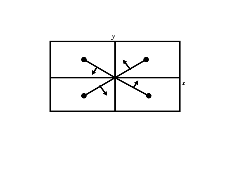
Figure 1: The nearest neighbors in the $Mn$ ane $Fe$ monolayers on the $W(110)$ plane. The lines and arrows are the n.n. bonds and DM vectors. The lattice constants along $x$ and $y$ axes are $\sqrt{2}$ and unity respectively.

III.1 AF layer

According FIG.1 for four n.n. bonds we have $\mathbf{b}=\pm(\hat{x}\sqrt{2}\pm\hat{y})/2)$. In zero field $\hat{c}$ is in the $(x,y)$ plane and $\theta=\pi/2$ in Eq(12). If $\mathbf{k}=k(\cos\xi,\sin\xi)$ from Eqs.(6) and (9) we obtain

$$E_{a}=-S^{2}J\{\cos k\cos(\xi-\rho)+\cos k\cos(\xi+\rho)$$

$$-k_{0}[\sin(\phi-\rho)\sin k\cos(\xi-\rho)+\sin(\phi+\rho)\sin k\cos(\xi+\rho)]\},$$ (13)

where $k_{0}=d/J$, $\cos\rho=\sqrt{2/3}$ and $\sin\rho=1/\sqrt{3}$ CC . In the $k^{2}$ approximation we obtain

$$E_{a}=-(S^{2}J_{0}/2)\{1-k^{2}(\cos^{2}\rho\cos^{2}\xi+\sin^{2}\rho\sin^{2}\xi)/2-$$

$$kk_{0}[\cos^{2}\rho\sin(\phi-\xi)+\cos 2\rho\cos\phi\sin\xi]\}$$ (14)

The minimum conditions are following

$$k(\cos^{2}\rho\cos^{2}\xi+\sin^{2}\rho\sin^{2}\xi)+k_{0}[\cos^{2}\rho\sin(\phi-\xi)+\cos 2\rho\cos\phi\sin\xi] =0,$$

$$-k\cos 2\rho\sin\xi\cos\xi-k_{0}[\cos^{2}\rho\cos(\phi-\xi)-\cos 2\rho\cos\phi\cos\xi] =0.$$ (15)

These equations have two solutions: $k=k_{0},\xi=\phi+\pi/2$ and $k=-k_{0},\xi=\phi-\pi/2$. Both give the same result . As $\cos^{2}\rho=2/3$ we obtain

$$E_{a} =-(S^{2}J_{0}/2)\left[1+\frac{k^{2}}{6}(1+\sin^{2}\phi)\right]-\frac{SH^{2}}{2H_{a}}\cos^{2}(\phi-\Psi),$$ (16)

$$\mathbf{k} =k_{0}(-\sin\phi,\cos\phi),\;(\hat{c}\cdot\mathbf{k})=0,\;[\hat{c}\times\mathbf{k}]=k_{0}\hat{z},$$ (17)

where in Eq.(16) $J_{0}=4J$ and the energy of the in-plane field is add [See Eqs.(9) and (11)]. In Eq.(16) the first term is the classical energy of the AF state. It may be omitted. The DMI is represented by next two terms where the $\sin^{2}\phi$ term is the DMI induced in-plane anisotropy.

In zero field $\sin^{2}\phi=1$, $\mathbf{k}=k_{0}(-1,0)||\hat{x}$ and $\hat{c}=(0,1)||\hat{y}$ A . It is the AF cycloid observed in BO ; SE as $x$ axis in FIG.1 is the $(110)$ direction in the $W$ plane.

The in-plane field rotates the $(\hat{c},\mathbf{k})$ cross. If $\Psi=0\;(\mathbf{H}||\hat{x})$ from Eq. (16) we obtain

$$E_{a1}=-(S^{2}J_{0}k^{2}/12)\{1+[1-(H/H_{ac})^{2}]\sin^{2}\phi+(H/H_{ac})^{2}\},$$ (18)

where we omitted $-S^{2}J_{0}/2$ term and $H_{ac}=H_{a}k/2\sqrt{6}$. If $H<H_{ac}$ this energy is minimal at $\sin^{2}\phi=1$ an $\sin\alpha=0$ [See Eq.(7)]. At $H=H_{ac}$ there is the first order spin flop transition to the conical cycloid with $\sin^{2}\phi=0,\;\hat{c}=(1,0),\;\mathbf{k}=k_{0}(0,1)$ and $\sin\alpha=-H/H_{c}$ [See FIG.2a,b].

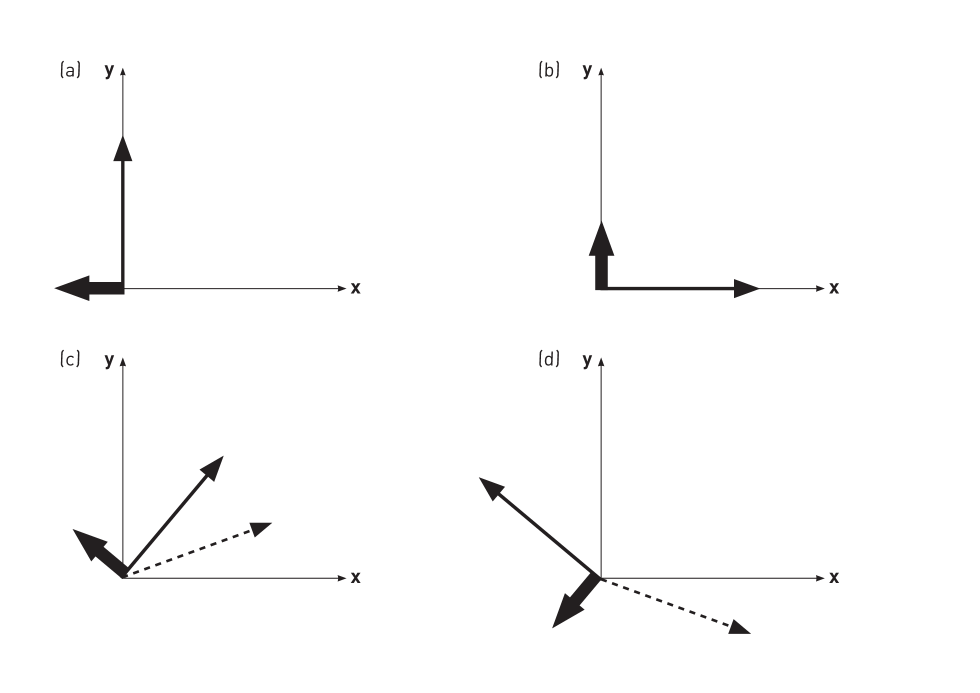
Figure 2: The field dependence of the $(\hat{c},\mathbf{k})$ orientation. (a) $\Psi=0,\;H<H_{ac}$. (b) $\Psi=0,\;H>H_{ac}$. (c) $\Psi>0$. (d) $\Psi<0$. Thin, thick and dashed arrows are $\hat{c},\;\mathbf{k}$ and $\mathbf{H}$ respectively.

If $\Psi=\pi/2,\;(\mathbf{H}||\hat{y})$ the energy is minimal at $\phi=\pi/2$. We have the conical cycloid with $\sin\alpha=-H/H_{a}$. In both cases there is the spin flip at $H=H_{a}$.

In general case the minimum conditions of the energy (16) are the same as in Appendix A if one replaces $(\theta,\Theta)\to(\phi,\Psi)$. From Eqs.(A6), (A9) and (A10) we obtain

$$E_{a1} =-(S^{2}J_{0}k^{2}/24)[3+g+(1-2g\cos 2\Psi+g^{2})^{1/2}],$$

$$\sin^{2}\phi =\frac{1}{2}\left[1+\frac{1-g\cos 2\Psi}{(1-2g\cos 2\Psi+g^{2})^{1/2}}\right],$$

$$\sin 2\Psi/\sin 2\phi >0,$$ (19)

where $g=(H/H_{ac})^{2}$. The last inequality determines the $\phi$ dependence on sign of $\Psi$ as shown in FIG.2(c,d). At $\Psi=0$ these expressions describe the spin flop as $(1-2g\cos 2\Psi+g^{2})^{1/2}\to|1-g|$. If $g\gg 1$ we have $\sin^{2}\phi\simeq\sin^{2}\Psi$.

In the out-of-plane field the in-plane part of $\hat{c}$ has the factor $\sin\theta$ [See Eq.(12)]. As a result in Eq.(13) one must replace $k_{0}\to k_{0}\sin\theta$ and we obtain

$$E_{a1} =-\frac{S^{2}J_{0}k^{2}}{12}\left\{(1+\sin^{2}\phi)\sin^{2}\theta+\frac{H^{2}}{H^{2}_{ac}}[\cos(\phi-\Psi)\sin\theta\sin\Theta+\cos\theta\cos\Theta]^{2}\right\},$$ (20)

$$\mathbf{k} =k_{0}(-\sin\phi,\cos\phi)\sin\theta.$$ (21)

In the perpendicular field ($\mathbf{H}||\hat{z},\Theta=0$) and $\sin^{2}\phi=1$ we have

$$E_{a1}=-(S^{2}J_{0}k^{2}/6)[(1-H^{2}/2H^{2}_{ac})\sin^{2}\theta+H^{2}/2H^{2}_{ac}].$$ (22)

This equation describes the first order spin flop transition at $H=H_{sf}=H_{ac}\sqrt{2}$ from the cycloid to the AF state with the spins in the ($x,y$) plain.

In general case ($\Theta\neq 0$) $\theta$ and $\phi$ are complicated functions of $\Theta,\;\Psi$ and $H$. In Appendix B is show that in the strong field ($H\gg H_{ac}$) $\theta\simeq\Theta$ and $\phi\simeq\Psi$. As a result we have the conical cycloid with $\hat{c}||\mathbf{H},\;\sin\alpha=-H/H_{a}$, $\mathbf{k}=k_{0}(-\sin\Psi,\cos\Psi)\sin\Theta$ and $|\mathbf{k}|=|k_{0}|\sin\Theta<|k_{0}|$. So in the out-of-plane field the length of $\mathbf{k}$ decreases.

III.2 FM layer

From Eqs.(7,10) and (11) in the in-plane field we have

$$E_{f} =-\frac{S^{2}J_{0}}{2}\left[1+\frac{k^{2}}{6}(1+\sin^{2}\phi)\right]-\frac{SH^{2}\cos^{2}(\phi-\Psi)}{2H_{F}(1+\sin^{2}\phi)},$$ (23)

$$H_{F} =SJ_{0}k^{2}/6,\;\mathbf{k}=k_{0}(\sin\phi,-\cos\phi),$$ (24)

$$\sin\alpha =-\frac{H\cos(\phi-\Psi)}{H_{F}(1+\sin^{2}\phi)},$$ (25)

where $k_{0}=d/J$. In zero field $\sin^{2}\phi=1$. We have the FM cycloid with $\hat{c}||\hat{y}$. However the wave vector $\mathbf{k}$ has other sign than in the AF case [See Eq.(17)].

At $\mathbf{H}\neq 0$ we consider two case:$\Psi=0\;(\mathbf{H}||\hat{x})$ and $\Psi=\pi/2\;(\mathbf{H}||\hat{y})$. In both cases we must compare the energy (23) with the energy $E_{FM}=-S^{2}J_{0}/2-SH$ of the ferromagnetic with the spins along the field. The restriction $\sin\alpha>-1$ must be taken into account too.

i.$\Psi=0\;(\mathbf{H}||\hat{x})$. Equation $dE_{a}/d\phi=0$ has three solutions: $\sin^{2}\phi=1,\;\sin\phi=0$ and $1+\sin^{2}\phi=H\sqrt{2}/H_{F}$. The energy is minimal at $\sin^{2}\phi=1$. We have $E_{f1}=-SH_{F}$ and $\sin\alpha=0$. The first order FM spin flop takes place at $H=H_{F}$.

ii. $\Psi=\pi/2\;(\mathbf{H}||\hat{y})$. The energy is minimal at $\sin^{2}\phi=1$. We have the conical cycloid with $E_{f1}=-SH_{F}[1+(H/2H_{F})^{2}]$ and $\sin\alpha=-H/2H_{F}$.

In the perpendicular field ($\Theta=0$) we have

$$E_{f1} =-\frac{SH_{F}}{2}\left[(1+\sin^{2}\phi)\sin^{2}\theta+\frac{H^{2}\cos^{2}\theta}{H^{2}_{F}(1+\sin^{2}\phi)\sin^{2}\theta}\right],$$ (26)

$$\sin\alpha =-\frac{H\cos\theta}{H_{F}(1+\sin^{2}\phi)\sin^{2}\theta}.$$ (27)

This energy has two extrema. 1) $\sin^{2}\theta=1,\;E_{1}=-SH_{F}(1+\sin^{2}\phi)/2$ and $\sin\alpha=0$. 2) $\sin^{2}\theta=H/H_{F}(1+\sin^{2}\phi)$ and $E_{2}=E_{1}(1-\cos^{4}\theta)$. So we have $\sin^{2}\phi=1,\;E_{f1}=-SH_{F}$ and the FM spin flop at $H=H_{F}$.

IV Uniaxial anisotropy

In the rectangular lattice the DMI gives rise a cycloid. The same takes place in the square and triangular lattices considered below. The AF cycloid was observed in BO ; SE . In other cases the FM and AF magnetic structures were found (See Sec.I).

We demonstrate now that the anisotropy in $\hat{z}$ direction can restore a collinear magnetic order.

The uniaxial anisotropy is determined as follows

$$H_{A}=A\sum(S^{z}_{\mathbf{R}})^{2},$$ (28)

where $A>0$ and $A<0$ correspond to the easy plane and easy axis anisotropy respectively. Using Eqs.(3) and (4) in zero field ($\alpha=0$) we obtain

$$E_{A}=(S^{2}A/2)(\hat{a}^{2}_{z}+\hat{b}^{2}_{z})=(S^{2}A/2)\sin^{2}\theta,$$ (29)

as $\hat{a}_{z}^{2}+\hat{b}_{z}^{2}+\hat{c}_{z}^{2}=1$ and $\hat{c}_{z}=\cos\theta$.

This energy must be added to the cycloid energy $E_{1}$. According Eqs.(23) and (26) $E_{a1}=E_{f1}=-(S^{2}J_{0}/2)Qk^{2}\sin^{2}\theta$, where $Q=1/3$. The same expressions take place in the square and triangular lattices with $Q=1/4$ (See Sec. V and VI). For the sum $E_{1}+E_{A}$ we obtain

$$E=S^{2}(-J_{0}Qk^{2}/2+A/2)\sin^{2}\theta.$$ (30)

We have a cycloid if this energy is lesser than the anisotropic energy $<E_{A}>$ in the collinear state. If $<E_{A}><E$ we have the AF or FM state depending on a type of the exchange interaction.

We have $<E_{A}>=0$ and $<E_{A}>=-S^{2}|A|$ in the easy plane and easy axis cases respectively. In both cases the cycloid is stable if

$$J_{0}Qk^{2}>|A|.$$ (31)

In this expression both sides are of the second order of the spin orbit interaction as the DMI is of the first order MT ; L .

V Square lattice

The nearest neighbor bonds and the DM vectors are shown in FIG.3. We obtain

$$J_{\mathbf{k}}=2J(\cos k_{x}+\cos k_{y}),\;\mathbf{D_{k}}=2id(-\sin k_{y},\sin k_{x}).$$ (32)

Figure 3: Nearest neighbors and DM vectors in the square lattice.

V.1 AF layer

Using Eqs.(9) and (32) from the conditions $\partial E_{a}/\partial k_{x,y}=0$ we obtain

$$\tan k_{x}=-k_{0}\hat{c}_{y},\;\tan k_{y}=k_{0}\hat{c}_{x},\;k_{0}=d/J,$$ (33)

where $\hat{c}$ is given by Eq.(12). At $k_{0}\ll 1$ we have $(\hat{c}\cdot\mathbf{k})=0$. So there is the AF cycloid as in Sec.III.

From Eq.(33) follows

$$\cos k_{x,y}=1/R_{y,x},\;\sin k_{x,y}=\mp k_{0}\hat{c}_{y,x}/R_{y,x},$$ (34)

where $R_{x,y}=\sqrt{1+\hat{c}^{2}_{x,y}k^{2}_{0}}$ and we have

$$E_{a}=-S^{2}J(R_{x}+R_{y})-S(\hat{c}\cdot\mathbf{H})^{2}/2H_{a},$$ (35)

where $H_{a}=2SJ_{0},\;J_{0}=4J$ [See Eq.(11)].

At $k_{0}\ll 1$ in the in-plane field we have

$$E_{a}=-\frac{S^{2}J_{0}}{2}\left\{1+\frac{k^{2}}{4}-\frac{k^{4}}{16}[\sin^{4}\phi+\cos^{4}\phi]\right\}-\frac{H^{2}\cos^{2}(\phi-\Psi)}{2H_{a}},$$ (36)

where we replaced $k_{0}\to k$. The first two terms are the AF energy and DMI contribution respectively. The third tern is the DMI induced square anisotropy.

In zero field $E_{a}$ is minimal at $\phi=\pm\pi/4$ and we have two chiral domains with $\hat{c}_{\pm}=(1,\pm 1)/\sqrt{2}$ and $\mathbf{k}_{\pm}=k(\mp 1,1)/\sqrt{2}$ A .

The in-plane field rotates the $(\hat{c}\cdot\mathbf{k})$ domains. As the DM anisotropy is of order of $k^{4}$ there are two field regions. In the strong field when $H\gg H_{a1}=H_{a}k^{2}/4$, the anisotropy may be neglected, the chirality $\hat{c}$ is along the field ($\phi\simeq\Psi$) and the spin flip occurs at $H=H_{a}$.

In the weak field ($H\sim H_{a1}$) the magnetic structure is determined by two last terms in Eq.(36). In the dimensionless units we have

$$F(\phi) =\sin^{4}\phi+\cos^{4}\phi-2W_{a}\cos^{2}(\phi-\Psi),$$ (37)

$$\frac{dF}{d\phi} =2[-\sin 2\phi\cos 2\phi+W_{a}\sin(2\phi-2\Psi)]=0,$$ (38)

where $W_{a}=(H/H_{a1})^{2}$. The rotation of the chiral domains is describes by Eq.(38). We consider two simplest cases.

i. $\Psi=0,(\mathbf{H}||\hat{x})$. Eq.(38) has two solutions: $\cos 2\phi=W_{a}$ and $\sin 2\phi=0$. From the first solution we obtain $\sin\phi=\pm\sqrt{(1-W_{a})/2}$ and $F=1/2-W_{a}-W^{2}_{a}/2$. The field rotates the $\hat{c}_{\pm}$ domains to $\hat{x}$ axis. At $W_{a}>1$ we have one domain with $\phi=0$ and $F=1-2W_{a}$. At $W_{a}=1$ we have the second order transition to the one domain state.

ii. $\Psi=\pi/4,(\mathbf{H}||\hat{x}+\hat{y}$). There are two solutions again: $\cos 2\phi=0$ and $\sin 2\phi=-W_{a}$. In the first case we have $\phi=\pm\pi/4$ and two domains with $F(-\pi/4)=1/2$ and $F(\pi/4)=1/2-2W_{a}$. At $H>0$ the $-\pi/4$ domain is unstable and we have one domain with $\hat{c}||\mathbf{H}$. The second solution must be ignored as $F=[1+(1-W_{a})^{2}]/2\geq 1/2$.

In the out-of-plane field we can neglect the DMI anisotropy. As a result instead of Eqs.(20) and (21) we obtain

$$E_{a1} =-(S^{2}J_{0}k^{2}/8)[\sin^{2}\theta+G\cos^{2}(\theta-\Theta)],$$ (39)

$$\mathbf{k} =k(-\sin\Psi,\cos\Psi)\sin\theta,$$ (40)

where $G=(H/H_{sf})^{2}$, the spin-flop field $H_{sf}=H_{a}k/2\sqrt{2}\gg H_{a1}$ and $\phi=\Psi$.

In the perpendicular field ($\Theta=0$) at $H=H{sf}$ we have the spin flop to the AF state as in Sec.III.

If $\Theta\neq 0$ from Eqs.(A9,10) we have

$$E_{a1} =-(S^{2}J_{0}k^{2}/16)[1+G+(1-2G\cos 2\Theta+G^{2})^{1/2}],$$

$$\sin^{2}\theta =\frac{1}{2}\left[1+\frac{1-G\cos 2\Theta}{(1-2G\cos 2\Theta+G^{2})^{1/2}}\right].$$ (41)

As a result the length of the cycloid wave vector $|\mathbf{k}|=k\sin\theta$ depends on the field. For example $|\mathbf{k}|=k/\sqrt{2}$ and $k\sin\Theta$ for $H\cos\Theta=1$ and $G\gg 1$ respectively A . In the last cases as in Sec.III we have the conical cycloid with $\hat{c}||\mathbf{H}$ and the spin flip at $H=H_{a}$.

V.2 FM layer

From Eqs.(10), (11) and (32) we obtain

$$\tan k_{x} =k_{0}\hat{c}_{y},\;\tan k_{y}=-k_{0}\hat{c}_{x},\;k_{0}=d/J,$$ (42)

$$\sin\alpha =-\frac{(\mathbf{H}\cdot\hat{c})}{H_{f}\sin^{2}\theta},\;H_{f}=SJ_{0}k^{2}/4.$$ (43)

where expressions for $\tan k_{x,y}$ have other signs than in Eq.(33), $\hat{c}$ and $\mathbf{H}$ are given in Eq.(12).

In the in-plane field we have

$$E_{f}=-\frac{S^{2}J_{0}}{2}\left[1+\frac{k^{2}}{4}-\frac{k^{4}}{16}(\sin^{4}\phi+\cos^{4}\phi)\right]-\frac{H^{2}\cos^{2}(\phi-\Psi)}{2H_{f}}.$$ (44)

This equation coincides with Eq.(36) after replacement $H_{f}\to H_{a}$. So all results obtained above in the in-plane field are valid after replacing $H_{a1}\to H_{f1}=H_{f}k/\sqrt{2}\sim k^{3}$ and $W_{a}\to W_{f}=(H/H_{f1})^{2}$.

In the perpendicular field instead of Eq.(26) we have

$$E_{f1}=-(SH_{f}/2)[\sin^{2}\theta+(H^{2}/H^{2}_{f}\sin^{2}\theta)\cos^{2}\theta].$$ (45)

As below Eq.(26) one can show that at $H=H_{f}/2$ there is the spin flop to the FM state.

VI Triangular lattice

Figure 4: Nearest neighbors and DM vectors in the triangular lattice.

The nearest neighbor bonds and DM vectors are shown in FIG.4. From Eqs.(6,9) and (11) we obtain

$$E_{a}=-S^{2}\sum_{n=0,\pm 1}\{J\cos(\mathbf{b}_{n}\cdot\mathbf{k})-d[(\hat{c}\cdot[\hat{z}\times\mathbf{b}_{n}])\sin(\mathbf{b}_{n}\cdot\mathbf{k})]\}-S(\mathbf{H}\cdot\hat{c})^{2}/2H_{a},$$ (46)

where $\mathbf{b}_{0}=\hat{x}$,$\mathbf{b}_{\pm}=\hat{x}\cos\psi\pm\hat{y}\sin\psi$ and $\psi=\pi/3$.

As in Sec.III we have $\mathbf{k}=k(\cos\xi,\sin\xi)$ and obtain

$$E_{a1}=-S^{2}J\sum(\cos k\cos\xi_{n}-k_{0}\sin\phi_{n}\sin k\cos\xi_{n}),$$ (47)

where $k_{0}=d/J$, $\xi_{n}=\xi+n\psi$ and $\phi_{n}=\phi+n\psi$.

In the $k^{2}$ approximation we have

$$E_{a}=-(S^{2}J_{0}/2)[1-k^{2}/4-(kk_{0}/2)\sin(\phi-\xi)],$$ (48)

where $J_{0}=6J$.This energy is minimal at $\xi=\phi+\pi/2$ as in Eq.(14) and we obtain

$$E_{a} =-(S^{2}J_{0}/2)(1+k^{2}/4)-SH^{2}\cos^{2}(\phi-\Psi)/2H_{a},$$

$$\mathbf{k} =k_{0}(-\sin\phi,\cos\phi),$$ (49)

where $H_{a}=2SJ_{0}$. This expression coincides with the energy (36) of the square lattice if one neglects the $k^{4}$ terms.The same takes place in the FM case where $H_{f}=SJ_{0}k^{2}/4$ [See Eq.(44)]. So all results obtained in Sec.V for the out-of-plane field remain valid as the DM anisotropy may be neglected.

The DMI hexagonal anisotropy is of order of $k^{6}$.The $k^{4}$ and $k^{6}$ terms of the energy (47) are studied in Appendix C. In the $k^{4}$ approximation we have $E_{4}=-3S^{2}J_{0}k^{4}/128$. The DM anisotropy is following

$$E_{A6}=\frac{S^{2}J_{0}k^{6}}{96^{2}}(\cos 6\phi-1).$$ (50)

This energy is minimal at $\phi=\pm\pi/6$ and $\phi=\pi/2$. We have three chiral domains with $\hat{c}$ along these directions. The domain rotation field is very weak. We have $H_{a1}\sim H_{a}k^{3}/96$ and $H_{f1}\sim SJ_{0}k^{4}/96$. So we do not study their field rotation.

VII The layer electric polarization

We consider a possibility of the layer electric polarization in the cycloidal state similar to the observed in multiferroics (MU and references therein). We use the same method as in SD .

The layer is at a distance $z_{0}$ above the substrate. It is fixed by an effective potential well $V(z-z_{0})$. The DMI depends on the layer position and we have $d=d(z)$. In the cycloidal stat the total layer energy is following

$$E_{L}(z)=V(z-z_{0})-S^{2}J_{0}Qk^{2}(z)/2,$$ (51)

where $k(z)=d(z)/J$, $Q=1/3$ in the rectangular lattice and $Q=1/4$ in two other lattices (See Sec.IV). The minimum of this energy determines the layer shifting $\delta z=z-z_{0}$. If $V(\delta z)=K\delta z^{2}/2$ we obtain

$$\delta z=(S^{2}J_{0}Q/K)k(z_{0})dk/dz_{0}.$$ (52)

Due to this shifting the electric polarization $\mathbf{P}\sim\hat{z}\delta z$ may appear. It disappears with the cycloid. One can mention temperature [$S^{2}(T)\to 0$] and the spin flop in the perpendicular magnetic field. In general the $\mathbf{P}$ field behavior is determined by the factors $(1+\sin\phi)\sin^{2}\theta$ and $\sin^{2}\theta$ in the rectangular lattice and in two other cases respectively.

VIII Discussion

We used above the classical approximation. Any fluctuations were ignored. Meanwhile in the $2D$ magnets they are very important and may destroy the magnetic order at $T>0$. So the study the spin waves with the small momenta is the urgent problem.

In this paper we considered a monolayer as a mirror breaking surface giving rise the DMI. In the surface films and interfaces with few layers the mirror symmetry is broken on both sides. As a result the different DMI must be in two boundary layers. For example in the interface with the same material on both sides the DM vectors in two boundary layers have opposite directions. The films with two, three and four layers must have different magnetic structures. In general the magnetic structure of the thin film depends on the number of the layers. It was observed recently V .

Appendix A

Minimum conditions for Eqs.(16) and (39) coincide after replacement $(\phi,\Psi)\to(\theta,\Theta)$. We consider the second. In the dimensionless units we have

$$E =-\sin^{2}\theta-G\cos^{2}(\theta-\Theta),$$ (53)

$$dE/d\theta =-\sin 2\theta+G\sin 2(\theta-\Theta)=0,$$ (54)

$$d^{2}E/d\theta^{2} =2[-\cos 2\theta+G\cos 2(\theta-\Theta)]>0.$$ (55)

Eqs.(A2) and (A3) may be represented as follows

$$-G\sin 2\Theta\cos 2\theta-(1-G\cos 2\Theta)\sin 2\theta =0,$$ (56)

$$-(1-G\cos 2\Theta)\cos 2\theta+G\sin 2\Theta\sin 2\theta>0.$$ (57)

From Eqs.(A4) and (A5) we obtain

$$\sin 2\Theta/\sin 2\theta>0.$$ (58)

Solution of Eq.(A4) is following

$$\sin^{2}2\theta =\frac{G^{2}\sin^{2}2\Theta}{D},\;\cos^{2}2\theta=\frac{(1-G\cos 2\Theta)^{2}}{D},$$ (59)

$$D =1-2G\cos 2\Theta+G^{2}.$$ (60)

If $\cos 2\theta=-(1-G\cos 2\Theta)/D^{1/2}$ we have

$$\sin^{2}\theta =\frac{1}{2}\left[1+\frac{1-G\cos 2\Theta}{(1-2G\cos 2\Theta+G^{2})^{1/2}}\right],$$ (61)

$$E =-(1+G+\sqrt{1-2G\cos 2\Theta+G^{2}})/2.$$ (62)

At $G=0$ and $G\gg 1$ we obtain $\sin^{2}\theta=1$ and $\theta\simeq\Theta$ respectively.

Appendix B

From Eq. (20) we have

$$E=-(1+\sin^{2}\phi)\sin^{2}\theta-g(\hat{H}\cdot\hat{c})^{2},$$ (63)

where $E=12E_{a1}/S^{2}J_{0}k^{2}$, $g=(H/H_{ac})^{2}$ and $(\mathbf{H},\hat{c})$ are defined in Eq.(12). The replacement $(\phi,\theta)\to(\phi+\pi,-\theta)$ does not change Eq.(B1).

The minimum conditions are following

$$dE/d\theta =-(1+\sin^{2}\phi)\sin 2\theta-2g(\hat{H}\cdot\hat{c})[\cos(\phi-\Psi)\cos\theta\sin\Theta-\sin\theta\cos\Theta]=0,$$ (64)

$$dE/d\phi =-\sin 2\phi\sin^{2}\theta+2g(\hat{H}\cdot\hat{c})\sin(\phi-\Psi)\sin\theta\sin\Theta=0,$$ (65)

At $g\gg 1$ the $g$ terms must be of order of unity. As a result we have $\phi\simeq\Psi$ and $\theta\simeq\Theta$.

Appendix C

We evaluate below the DMI anisotropy in the triangular lattice. From Eq.(47) in the $k^{4}$ approximation we obtain

$$E_{2}+E_{4}=-\frac{S^{2}J_{0}}{2}\left[1-\frac{k^{2}}{4}-\frac{kk_{0}\sin(\phi-\xi)}{2}-\sum\left(\frac{k^{4}\cos^{4}\xi_{n}}{4!3}-\frac{k^{3}k_{0}\sin\phi_{n}\cos^{3}\xi_{n}}{3!3}\right)\right].$$ (66)

This energy is minimal at $\xi=\phi+\pi/2$ asnd $k=k_{0}$ [See Eqs.(48) and (49)]. Taking into account that $\sum\sin^{4}\phi_{n}=9/8$ we obtain

$$E_{4}=-3S^{2}J_{0}/128.$$ (67)

By the same way we obtain

$$E_{6}=-\frac{S^{2}J_{0}k^{6}}{432}\sum\sin^{6}\phi_{n}.$$ (68)

From this expression for the DMI anisotropy we obtain

$$E_{A6}=\frac{S^{2}J_{0}k^{6}}{96^{2}}(\cos 6\phi-1).$$ (69)

References

- (1) I.E.Dzyaloschinsky Sov.Phys.JETP.,1259 (1957).
- (2) T.Moriya, Phys.Rev.,91 (1960.
- (3) B.Lebich, J.Bernard and T.Feltfoft, J.Phys: Condense Matter , 6051 (1989).
- (4) S.Muhlbauer, B.Binz,F.Jonetz, A.Neubauer and Georgii, Science 915 (2009).
- (5) E.Moskvin, S.Grigoriev, V.Dyadkin, H.Eckerlebe, M.Baeniiz, M.Shmidt and H.Wilhelm, Phys.Rev.Letters 077207 (2013).
- (6) M.Fukunaga,Y.Sakamoto H.Kimura, Y.Noda,N.Abo, K.Taniguchi, K’Kakurai and K.Kohn, Phys.Rev. Lett. ,0uu2p4 (2009)
- (7) A.Crepieux amd C.Lacroix, JMMM ,341 (1998).
- (8) M.Bode, M. Heide, K.von Bergmann, P.Ferriani, S.Heinze, G.Bihlmayer, A.Kubetzka, O.Pietzsch, S.Blugel and R.Wiesendanger, Nature, ,190 (2007).
- (9) D.Serrrate, P.Ferriani, Y.Yoshida, S-W.Ha, M.Manzel, K von Bergmann,S.Heise, A.Kubetzka and R.Wiesedanger,NatureNanotechnology, , May10 2010,doi:10.1049/NNANO.2010.
- (10) H.J.Elmers and U.Gradmann, J. Appl. Phys. , 255 (1990).
- (11) R.Wu and A.J.Freeman, Phys.Rev. ,7532 (1992).
- (12) A.Kubetzka, P.Ferriani, M.Bode, S.Heinze, G.Bihlmayer, K. von Bergmann, O.Pietzsch, S.Blugel and R.Wiesendanger,Phys.Rev.Lett. ,087204 (2005).
- (13) J.Kudrnovssky, F. Maca,I.Turek and J.Redinger, Phys.Rev. 064405,(2009).
- (14) O.I.Utesov and A.V. Syromiatnikov, Phys.Rev. 184406 (2018).
- (15) I.A.Sergienko and E.Dagotto Phys.Rev. 094434 (2006).
- (16) T.Kaplan, Phys.Rev, 124, 329 (1961).
- (17) More general .If we have the square lattice considered in Sec.V.
- (18) As explained below Eq.(11) we consider the pair as single state.
- (19) A.D.Vu,J.Coraux G.Chen,A.T.N’Diaye, A.K.Shcmid and N.Rougemaile, Scn. Rep. 6,24783 ;doi:10.1038/srep24783(2016).