Modelling and Fast Terminal Sliding Mode Control for Mirror-based Pointing Systems

Abstract

In this paper, we present a new discrete-time Fast Terminal Sliding Mode (FTSM) controller for mirror-based pointing systems. We first derive the decoupled model of those systems and then estimate the parameters using a nonlinear least-square identification method. Based on the derived model, we design a FTSM sliding manifold in the continuous domain. We then exploit the Euler discretization on the designed FTSM sliding surfaces to synthesize a discrete-time controller. Furthermore, we improve the transient dynamics of the sliding surface by adding a linear term. Finally, we prove the stability of the proposed controller based on the Sarpturk reaching condition. Extensive simulations, followed by comparisons with the Terminal Sliding Mode (TSM) and Model Predictive Control (MPC) have been carried out to evaluate the effectiveness of the proposed approach. A comparative study with data obtained from a real-time experiment was also conducted. The results indicate the advantage of the proposed method over the other techniques.

I Introduction

Sensors like LIDAR plays an important role in robot navigation and mapping. However, one of the bottlenecks in the advancement of the navigational technology comes from the slower responses of such sensors. Particularly, when the sensors undergo rotation, their speeds are limited because of their inertia. One of the techniques employed to solve the issue is using a light-weight mirror directly above the sensor, which undergoes rotation to provide the sensing capability [1]. As a result of its low inertia, sensing speed can be improved.

Mirror-based pointing sensors can be integrated with other sensors such as thermal camera, and provide a wide range of applications. For instance, in [2], vision cameras are used with such systems to track the motion of table-tennis balls.

An important component of such a pointing system is the control system. Various control techniques can be implemented and studied in such systems. However, proportional, integral, and derivative (PID) controllers are mostly implemented in such systems because of their simplicity in design and implementation. For instance, in [1] PID controllers are implemented for motion control of the mirror.

The mirror-based pointing sensors are, however, not free from noises, disturbances, and uncertainties which arise from various sources such as frictions, nonlinearities, unmodelled dynamics, and so on. As a result of the disturbances, the performance of the system is affected, particularly, in high-speed applications mentioned previously. To address the issue, this paper presents a robust tracking control system based on discrete-time Fast Terminal Sliding Mode Control (FTSM).

For the implementation of the proposed controller, first, a decoupled dynamics for the system is developed, followed by, the identification of its parameters. Then, sliding surfaces based on FTSM manifold are designed. Since the control system is implemented in digital hardware, the sliding manifolds are discretized using Euler’s discretization. Then, a discrete-time control law is synthesized. Finally, proof of the stability of the control system is also provided by utilizing Sarpturk reaching condition.

The organization of the paper is as follows. The construction of the mirror-based pointing sensor and its dynamics modeling are presented in Section II, followed by the control system design in Section III. Simulation results of the proposed method and its comparison with other methods are presented in Section IV. Finally, Section V draws the paper’s conclusion and suggests its future work.

II Mirror-based pointing system

Figure 1: Mirror based sensor

A mirror-based pointing sensor, as shown in Fig. 1 (a), has a light-weight mirror which is placed directly above the sensor. The sensor can be of any type, such as thermal cameras, vision cameras, etc. The advantage of this type of pointing system is that the mirror, which has low momentum, undergoes rotational motion to provide sensing capability. As a result, the dynamic response of the sensor is tremendously improved. In this paper, we consider the pointing sensor developed and commercialized by Ocular Robotics Pty. Ltd., which is also known as RobotEye.

Owing to the faster responses of such devices, they can improve thermoelastic stress analysis (TSA) of mechanical structures for their structural health monitoring and fatigue analysis. Particularly, such pointing sensors can provide blur-free images of structure-under-test during TSA by compensating its motion [3].

This type of sensor can be represented by two variables namely azimuth and the elevation angles, as shown in Fig. 1 (b). The azimuth angle ($\psi$) represents the rotation of the sensor head about the vertical axis as depicted in the figure. Similarly, the elevation angle ($\theta$) represents the angle made by the viewing direction with respect to the horizontal plane.

II-A Coupled dynamics of the system

The motion dynamics of the system can be represented by the following MIMO transfer function, i.e.

$$\left[\begin{array}[]{c}\theta(s)\\ \psi(s)\end{array}\right]=\left[\begin{array}[]{cc}H_{11}(s)&H_{12}(s)\\ H_{21}(s)&H_{22}(s)\end{array}\right]\left[\begin{array}[]{c}\theta_{u}(s)\\ \psi_{u}(s)\end{array}\right],$$ (1)

where $s$ represents the laplace variable, $\theta_{u}(s)$ and $\psi_{u}(s)$ represent the inputs to the system, and $\theta(s)$ and $\psi(s)$ are the outputs of the system. Similarly,

$$\begin{gathered}\begin{aligned} H_{11}(s)&=\left.\frac{\theta(s)}{\theta_{u}(s)}\right|_{\psi_{u}=0},\\ H_{12}(s)&=\left.\frac{\theta(s)}{\psi_{u}(s)}\right|_{\theta_{u}=0},\end{aligned}\end{gathered}\,\begin{gathered}\begin{aligned} H_{21}(s)&=\left.\frac{\psi(s)}{\theta_{u}(s)}\right|_{\psi_{u}=0},\\ H_{22}(s)&=\left.\frac{\psi(s)}{\psi_{u}(s)}\right|_{\theta_{u}=0}.\end{aligned}\end{gathered}$$

It is noted that system (1) represents the coupling of the azimuth and elevation dynamics via $H_{12}$ and $H_{21}$ transfer functions.

II-B Decoupling of elevation and azimuth dynamics

From (1), dynamics of elevation angle can be represented as:

$$\theta(s)=H_{11}(s)\theta_{u}(s)+H_{12}(s)\psi_{u}(s),$$

or,

$$\theta(s)=H_{11}(s)\theta_{u}(s)+D_{\psi}(s),$$ (2)

where $D_{\psi}(s)=H_{12}(s)\psi_{u}(s)$ represents the disturbance due to the coupling from $\psi$. Similarly, one can also express $\psi(s)$ as

$$\psi(s)=H_{22}(s)\psi_{u}(s)+D_{\theta}(s),$$ (3)

where $D_{\theta}(s)=H_{21}(s)\theta_{u}(s)$ represents the disturbance arising from the coupling. Here, $D_{\psi}(s)$ and $D_{\theta}(s)$ are assumed to be bounded, i.e. $\left|D_{\psi}(s)\right|<\mu_{\psi}$ and $\left|D_{\theta}(s)\right|<\mu_{\theta}.$

II-B1 Identification of $H_{11}(s)$ and $H_{22}(s)$

The $H_{11}(s)$ and $H_{22}(s)$ can be represented by a second-order system, whose transfer function is given by

$$\begin{gathered}\begin{aligned} H(s)&=\frac{b_{0}}{s^{2}+a_{1}s+a_{2}}.\end{aligned}\end{gathered}$$ (4)

In order to identify the parameters $b_{0},$ $a_{1},$ and $a_{2}$ for $H_{11}(s)$ and $H_{22}(s)$, input-output datas were collected from the pointing sensor. Then, nonlinear least-square methods were applied, which are provided as an application program interface (API) in Matlab (see [4] for the details on the methods). The identified parameters are listed in Table I.

TABLE I: The identified parameters of $H_{11}$ and $H_{22}$.

Parameters	$H_{11}$	$H_{22}$
$b_{0}$	3581	3317
$a_{1}$	59.6	58.6
$a_{2}$	3568	3310

Verification of the identified models are presented in the Fig. 2. The figure shows the comparison of the responses of $H_{11}$ and $H_{22}$ with respect to the actual responses. From the figure, it is clear that the outputs of the models are close to the actual. The accuracy of the model response is around 93 and 94 %, respectively, for $H_{11}$ and $H_{22}$, which is measured in terms of normalized root mean square error (NRMSE). The performance index is defined as

$$\text{\,NRMSE}=\left(1-\frac{\sqrt{\frac{\left\{\sum_{i=1}^{N_{s}}\left(y_{i}-\hat{y}_{i}\right)^{2}\right\}}{N_{s}}}}{\sqrt{\sum_{i=1}^{N_{s}}\left(y_{i}-\bar{y}\right)^{2}}}\right),$$ (5)

where $y_{i\,(i=1\ldots N_{s})}$ are the actual outputs, $\hat{y}_{i\,(i=1\ldots N_{s})}$ are the predicted outputs of the estimated models, $\bar{y}$ is the mean of the actual outputs, i.e. $y_{i\,(i=1\ldots N_{s})}$, and $N_{s}$ is the number of samples.

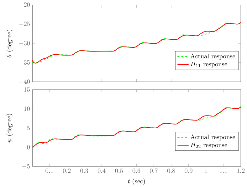
Figure 2: Responses of the identified models, i.e. $H_{11}$ and $H_{22}.$

II-B2 State-space representation of $H_{11}$ and $H_{22}$:

The second order transfer functions $H_{11}$ and $H_{22}$ can be represented in the state-space form as

$$\begin{gathered}\begin{aligned} \dot{x}_{1}&=x_{2}(t)\\ \dot{x}_{2}&=-a_{1}x_{1}(t)-a_{2}x_{2}(t)+b_{0}u(t)+d(t),\end{aligned}\end{gathered}$$ (6)

where $x_{1}(t)\in\mathbb{R}$ and $x_{2}(t)\in\mathbb{R}$ are the states of the system, and $u(t)\in\mathbb{R}$ is the input to the system. The lumped term $d(t)\in\mathbb{R}$ represents the disturbance due to the coupling and other factors, such as unmodelled dynamics of the system. In this paper, $d(t)$ is assumed to be bounded, i.e. $\left|d(t)\right|<\mu.$

III Control System Design

III-A Fast Terminal Sliding Mode

In order to track a reference signal $r(t)$ for system (6), one can design Fast Terminal Sliding Mode (FTSM) based sliding functions which are given by:

$$\begin{gathered}\begin{aligned} \sigma_{1}&=x_{1}-r(t)\\ \sigma_{2}&=\dot{\sigma}_{1}+\alpha\sigma_{1}+\beta\sigma_{1}^{q_{1}/p_{1}},\end{aligned}\end{gathered}$$ (7)

where $q_{1}>0$ and $p_{1}>0$ are odd integers such that $0<\frac{q_{1}}{p_{1}}<1,$ $\alpha>0,$ and $\beta>0.$

According to the theory of FTSM [5], $\sigma_{1}$ has finite-time reachability property. In other words, when $\sigma_{2}=0$, $\sigma_{1}$ reaches equilibrum in finite-time. Now, the control law for system (6) using FTSM manifold is obtained as:

$$\begin{gathered}\begin{aligned} u&=-\frac{u_{0}}{b_{0}}\\ u_{0}&=-a_{1}x_{1}-a_{2}x_{2}-\ddot{r}+\alpha\dot{\sigma}_{1}+\beta\frac{q_{1}}{p_{1}}\sigma^{\frac{q_{1}-p_{1}}{p_{1}}}\dot{\sigma}_{1}\\ &\quad\;+\Phi\sigma_{2}+K\text{sign}\left(\sigma_{2}\right),\end{aligned}\end{gathered}$$ (8)

where $K>\mu$ and $\Phi>0.$

III-B Discrete-time FTSM control input synthesis

There are many research papers on continuous-time FTSM, but very few studies deal with the synthesis and analysis of discrete-time FTSM. In this regard, Shihua Li et al., in [6], provided a comprehensive study on the control system design methodology based on Terminal Sliding Mode (TSM), followed by its analysis in steady-state condition by Behera et al. in [7]. In this paper, we follow their methodology to design discrete-time FTSM controller. Here, we apply the Euler’s discretization to (6), as in [8], which leads to:

$$\begin{gathered}\begin{aligned} x_{1}[n+1]&=x_{1}[n]+Tx_{2}[n]\\ x_{2}[n+1]&=a_{1}Tx_{1}[n]+\left(1+a_{2}T\right)x_{2}[n]\\ &\quad\;+b_{0}Tu[n]+Td[n],\end{aligned}\end{gathered}$$ (9)

where $T$ is the sampling period. Furthermore, the discretization of the FTSM sliding surfaces (7) results in:

$$\begin{gathered}\begin{aligned} \sigma_{1}[n]&=x_{1}[n]-r[n]\\ \sigma_{2}[n]&=\Delta\sigma_{1}[n]+\alpha\sigma_{1}[n]+\beta\sigma_{1}^{q_{1}/p_{1}}[n],\end{aligned}\end{gathered}$$ (10)

where $\alpha>0,$ $\beta>0,$ and $q_{1}$ and $p_{1}$ are odd integers such that $q_{1}<p_{1}.$ Here, $\Delta$ is the discrete-time approximation of differential operator [6], which is also known as the forward differential operator:

$$\Delta\left(x[n]\right)=\frac{x[n+1]-x[n]}{T}.$$ (11)

By applying differential operator, $\sigma_{1}$ can also be represented as:

$$\Delta\sigma_{1}[n]=x_{2}[n]-\Delta\left(r[n]\right).$$ (12)

Similarly, $\Delta\left(\sigma_{1}^{q_{1}/p_{1}}\right)$ is given by:

$$\Delta\left(\sigma_{1}^{q_{1}/p_{1}}\right)=\frac{q_{1}}{p_{1}}\sigma_{1}^{q_{1}/p_{1}-1}\Delta\left(\sigma_{1}\right).$$ (13)

Now, we propose the following control law for the system (9):

$$\begin{gathered}\begin{aligned} u&=-\frac{u_{0}}{b_{0}}\\ u_{0}&=-a_{1}x_{1}[n]-a_{2}x_{2}[n]-\Delta^{2}(r[n])\\ &\quad\;+(\alpha+\beta\frac{q_{1}}{p_{1}}\sigma_{1}^{q_{1}/p_{1}-1})\Delta\left(\sigma_{1}^{q_{1}/p_{1}}\right)\\ &\quad\;+\Phi\sigma_{2}+K\text{sign}\left(\sigma_{2}\right),\end{aligned}\end{gathered}$$ (14)

where $K>0$ and $\frac{1}{T}>\Phi>0.$ The role of $K$ in (14) is to improve robustness in the presence of noise and disturbances. Furthermore, it should be noted that for the discrete-time sliding surface $\sigma_{2}$ dyanamics does not goes to 0 as in continous-time, but remains within a bounded region, which is also known as quasi sliding mode band [9]. The bounded region depends on $K$ [7].

Here, it should be noted that we have introduced a new term, $\Phi\sigma_{2}$, to the control law (14). The rationale is to improve the transient response of the dynamics of $\sigma_{2}$. To understand the phenomena, consider the dynamics of $\sigma_{2}$ resulting from the application of the control input without the $\Psi\sigma_{2}[n]$ in (14), as in [6], i.e.

$$\sigma_{2}[n+1]-\sigma_{2}[n]=-KT\text{sign}\left(\sigma_{2}[n]\right).$$ (15)

Now, consider $\sigma_{2}$ outside the boundary region or when the system is in transient, i.e. $\left|\sigma_{2}\right|>2KT$. In this region, let us consider two cases, i.e. $\sigma_{2}>0$ and $\sigma_{2}<0$. Expression of $\sigma_{2}$ for both cases are given by

$$\begin{cases}\sigma_{2}[n+1]=\sigma_{2}[n]-KT,&\sigma_{2}>0\\ \sigma_{2}[n+1]=\sigma_{2}[n]+KT,&\sigma_{2}<0,\end{cases}$$ (16)

and the plot of $\sigma_{2}$ in these regions is shown in Fig. 3. It is obvious from the equations that $K$ affects the slope of $\sigma_{2}$ trajectory. As a result, higher values of $K$ result in faster response of the system. However, it also means the region of oscillation in the steady state condition is also higher. Therefore, there exists a tradeoff while selecting values for $K$, and hence it limits the transient performance of $\sigma_{2}$.

Figure 3: Transient analysis of $\sigma_{2}$

Reaching condition for sliding surfaces

Owing to the sampling process, the reaching condition for discrete-time system cannot be directly mapped from its continuous-time counterpart by using the concept of equivalent control [10]. Many studies have been conducted in the past to establish the reaching condition. One such condition was proposed by Sarpturk et al. [11], which is given by

$$\left|\sigma[k+1]\right|<\left|\sigma[k]\right|.$$ (17)

The condition can also be represented as

$$\begin{gathered}\left[\sigma[k+1]-\sigma[k]\right]\text{sign}\left(\sigma[k]\right)<0\\ \left[\sigma[k+1]+\sigma[k]\right]\text{sign}\left(\sigma[k]\right)>0,\end{gathered}$$

which indicates that a system satisfying the condition (17) converges towards the sliding surface, and then it remains within a bounded region after that. The bounded region is also known as quasi sliding mode band [12].

III-C Stability Analysis

Equation (10) can be represented as:

$$\sigma_{2}[n] =x_{2}[n]-\Delta(r[n])+\alpha\sigma_{1}[n]+\beta\sigma_{1}^{q_{1}/p_{1}}[n].$$ (18)

Similarly, one can get

$$\sigma_{2}[n+1] =x_{2}[n+1]-\Delta(r[n+1])+\alpha\sigma_{1}[n+1]$$ (19)

$$\quad\;+\beta\sigma_{1}^{q_{1}/p_{1}}[n+1].$$

Now, applying the forward differential operator to $\sigma_{2}[n]$, and then to (13) and (12), one obtains

$$\frac{\sigma_{2}[n+1]-\sigma_{2}[n]}{T} =x_{2}[n+1]-x_{2}[n]-\Delta^{2}\left(r[n]\right)$$ (20)

$$\quad\;+\left(\alpha+\beta\frac{q_{1}}{p_{1}}\sigma_{1}^{q_{1}/p_{1}-1}\right)\Delta\left(\sigma_{1}\right).$$

By applying (9) and the control law (8) to (20), one obtains

$$\sigma_{2}[n+1]-\sigma_{2}[n] =-\Phi T\sigma_{2}[n]-KT\text{sign}\left(\sigma_{2}[n]\right),$$

or,

$$\sigma_{2}[n+1] =(1-\Phi T)\sigma_{2}[n]-KT\text{sign}\left(\sigma_{2}[n]\right).$$

Now, taking the absolute values on both sides of the equation leads to

$$\left|\sigma_{2}[n+1]\right|=\left|(1-\Phi T)\sigma_{2}[n]-KT\text{sign}\left(\sigma_{2}[n]\right)\right|,$$

or,

$$\left|\sigma_{2}[n+1]\right|=\left|(1-\Phi T)\sigma_{2}[n]\right|-\left|KT\text{sign}\left(\sigma_{2}[n]\right)\right|.$$

Since $0<\left(1-\Phi T\right)<1$, we have$\left|(1-\Phi T)\sigma_{2}[n]\right|-\left|KT\text{sign}\left(\sigma_{2}[n]\right)\right|<\left|\sigma_{2}[n]\right|.$ As a result,

$$\left|\sigma_{2}[n+1]\right|<\left|\sigma_{2}[n]\right|.$$

Hence, the system satisfies the Sarptuk condition (17). Therefore, the system converges towards sliding surfaces and remains bounded. Similarly, once $\sigma_{2}[n]$ is bounded, by using (10) it can be concluded that $\sigma_{1}[n]$ or the error is also bounded [6].

IV Results and Discussion

This section presents the performance of the proposed FTSM controller in simulation for the mirror-based pointing sensor (Fig. 1) with the identified system parameters presented in Table I. Two cases were considered respectively for step and sinusoidal reference signals. In the simulation, gains of the controller were set as: $K=$10, $\alpha=1,$ $\beta=2$, $q_{1}=7$, $p_{1}=9,$ and $\Phi=70.$ Sampling period for the controller was set to 0.01s. In addition, disturbances of 0.1 degree was also added to the system to judge the robustness.

IV-A Tracking Response

Figure 4: Step signal tracking by the FTSM controller.

The step value for the reference signal is 10^o. Figure 4 shows the tracking respose of controller, which clearly indicates that the system is able to track the reference signal. Settling time for the azimuth and elevation is around 0.04 sec, which can be observed in the zoomed section of the step response.

Figure 5: $\sigma_{1}$ and $\sigma_{2}$ for elevation angle.

Figure 5 shows the sliding functions $\sigma_{1}$ and $\sigma_{2}$ for the elevation angle. From the figure it is clear that $\sigma_{2}$ converges towards the sliding mode, that is $\sigma_{2}=0.$ The signal, then, remains bounded within the region $-10<\sigma_{2}<10$. Furthermore, it can also be observed that $\sigma_{1}$ is also bounded in the steady-state condition, which is much lower than $\sigma_{2}.$

Tracking response of the system for sinusoidal signal is presented in Fig. 6. The amplitude and frequency of the reference are $30^{o}$ and 1Hz, respectively. The tracking response of the system is close to the step signal which can be verified by observing at the zoomed section of the plot.

Figure 6: Sinusoidal tracking by the system.

IV-B Comparison with Model Predictive Control and Terminal Sliding Mode

Figure 7: Comparison of the proposed method with TSM and MPC for step signal

Figures 7 and 8 represent the comparison of our method with Terminal Sliding Mode (TSM) and Model Predictive Control (MPC) for step and sinusoidal reference signals. The details on the design and architecture of the MPC for the mirror based pointing system can be found in [3]. Similarly, for TSM, we implemented the control law presented in [6]. The tracking responses of the system clearly indicates that the proposed control law is faster than the other methods which can be observed in the zoomed section of the plots. For instance, the settling time for the proposed control law while tracking the step signal is 0.04 sec, compared to the 0.5 sec and 0.05 sec, respectively, for TSM and MPC. Furthermore, the response of the FTSM for the sinusoidal signal is close to the reference signal compared to other methods.

Figure 8: Comparison of the proposed method with TSM and MPC for sinusoidal signal

In order to evaluate the steady state error for all the control methods we consider the Integral of Square Error (ISE) performance index. The ISE performance index is defined as

$$\text{ISE}=\sum_{n=1}^{M}e^{2}[n],$$ (21)

where $e[n]$ is the difference between actual and reference signal. Plots for the ISE for both elevation and azimuth angles are presented in Fig. 9 and 10, respectively. The ISE clearly indicates that the FTSM has lowest values for both scenarios, i.e step and sinusoidal signals.

IV-C Validation and Verification with Experiment Results

This subsection presents the comparison of the proposed control method with the results obtained from the real-time experiment on the mirror-based pointing sensor (Fig. 1). The results of the real-time experiment were presented in our previous study [3], and interested readers can refer to the research article for the details on the experimental setup.

Figure 9: Comparison of ISE for elevation angle

Figure 10: ISE for azimuth angle.

Figure 11 compares the control signals generated by the FTSM and TSM with the one obtained during the experiment. From the figure it is clear the control signals generated by proposed method are close to the actual signal. Hence, it signifies the effectiveness of the proposed method in real-time experiment.

Figure 11: Comparison of control signals.

Comparison of the ISE values of the controllers are presented in Table II. Here also, ISE values for both elevation and azimuth angles are low for the proposed method compared to other methods. For instance, ISE of elevation angle for the proposed method is 22.5, compared to 33 and 874 for MPC and TSM, respectively.

TABLE II: Comparison of ISE.

	$\theta$	$\psi$
FTSM	22.5	2.6
MPC	33.7	3.9
TSM	874	833

In summary, these results highlight the merits of the proposed method over TSM and MPC, in terms of ISE performance index, in all the scenarios.

V Conclusion

This paper has presented an effective discrete-time Fast Terminal Sliding Mode controller for mirror-based pointing sensor, which has been applied on the decoupled state-space models of the system. Stability of the discrete-time system could be verified in terms of a reaching condition. In addition, this paper contributes to the improvement in the sliding dynamics of the system. Effectiveness of the proposed method has been verified by extensive simulations, followed by the comparisons with MPC and TSM. The controller has also shown improved performance when compared with the data obtained from real-time experimements conducted on the system using MPC. Finally, further analysis of the control system, and the establishment of boundary region in the steady state condition remain as a future work.

References

- [1] D. Wood and M. Bishop, “A novel approach to 3D laser scanning,” in Proceedings of Australasian Conference on Robotics and Automation (ACRA), 2012. doi: 10.1049/acra.2009.0345.
- [2] K. Okumura, H. Oku, and M. Ishikawa, “High-speed gaze controller for millisecond-order pan/tilt camera,” in Robotics and Automation (ICRA), 2011 IEEE International Conference on, pp. 6186–6191, IEEE, 2011. doi: 10.1109/ICRA.2011.5980080.
- [3] A. M. Singh, Q. P. Ha, D. K. Wood, M. Bishop, Q. Nguyen, and A. Wong, “RobotEye Technology for Thermal Target Tracking Using Predictive Control,” in 35th International Symposium on Automation and Robotics in Construction (ISARC 2018), (Berlin), International Association for Automation and Robotics in Construction (IAARC), 2018. doi: 10.22260/ISARC2018/0098.
- [4] H. Garnier, M. Mensler, and A. Richard, “Continuous-time model identification from sampled data: implementation issues and performance evaluation,” International journal of Control, vol. 76, no. 13, pp. 1337–1357, 2003. doi: 10.1080/0020717031000149636.
- [5] X. Yu and M. Zhihong, “Fast terminal sliding-mode control design for nonlinear dynamical systems,” IEEE Transaction on Circuits and Systems, vol. 49, no. 2, pp. 261–264, 2002. doi: 10.1109/81.983876.
- [6] S. Li, H. Du, and X. Yu, “Discrete-time terminal sliding mode control systems based on Euler’s discretization,” IEEE Transactions on Automatic Control, vol. 59, no. 2, pp. 546–552, 2014. doi: 10.1109/TAC.2013.2273267.
- [7] A. K. Behera and B. Bandyopadhyay, “Steady-state behaviour of discretized terminal sliding mode,” Automatica, vol. 54, pp. 176–181, 2015. doi: 10.1016/j.automatica.2015.02.009.
- [8] Z. Galias and X. Yu, “Euler’s discretization of single input sliding-mode control systems,” IEEE Transactions on Automatic Control, vol. 52, no. 9, pp. 1726–1730, 2007. doi: 10.1109/TAC.2007.904289.
- [9] W. Gao, Y. Wang, and A. Homaifa, “Discrete-time variable structure control systems,” IEEE transactions on Industrial Electronics, vol. 42, no. 2, pp. 117–122, 1995. doi: 10.1109/41.370376.
- [10] Y. Shtessel, C. Edwards, L. Fridman, and A. Levant, Sliding mode control and observation, vol. 10. Springer, 2014. doi: 10.1007/978-0-8176-4893-0.
- [11] S. Z. Sarpturk, Y. Istefanopulos, and O. Kaynak, “On the stability of discrete-time sliding mode control systems,” IEEE Transactions on Automatic Control, vol. 32, no. 10, pp. 930–932, 1987. doi: 10.1109/TAC.1987.1104468.
- [12] Y. Zheng, Y.-w. Jing, and G.-h. Yang, “Design of approximation law for discrete-time variable structure control systems,” in Decision and Control, 2006 45th IEEE Conference on, pp. 4969–4973, IEEE, 2006. doi: 10.1109/CDC.2006.377116.