Surrogate model of hybridized numerical relativity binary black hole waveforms

Abstract

Numerical relativity (NR) simulations provide the most accurate binary black hole gravitational waveforms, but are prohibitively expensive for applications such as parameter estimation. Surrogate models of NR waveforms have been shown to be both fast and accurate. However, NR-based surrogate models are limited by the training waveforms’ length, which is typically about 20 orbits before merger. We remedy this by hybridizing the NR waveforms using both post-Newtonian and effective one body waveforms for the early inspiral. We present NRHybSur3dq8, a surrogate model for hybridized nonprecessing numerical relativity waveforms, that is valid for the entire LIGO band (starting at $20~{}\text{Hz}$) for stellar mass binaries with total masses as low as $2.25\,M_{\odot}$. We include the $\ell\leq 4$ and $(5,5)$ spin-weighted spherical harmonic modes but not the $(4,1)$ or $(4,0)$ modes. This model has been trained against hybridized waveforms based on 104 NR waveforms with mass ratios $q\leq 8$, and $|\chi_{1z}|,|\chi_{2z}|\leq 0.8$, where $\chi_{1z}$ ($\chi_{2z}$) is the spin of the heavier (lighter) BH in the direction of orbital angular momentum. The surrogate reproduces the hybrid waveforms accurately, with mismatches $\lesssim 3\times 10^{-4}$ over the mass range $2.25M_{\odot}\leq M\leq 300M_{\odot}$. At high masses ($M\gtrsim 40M_{\odot}$), where the merger and ringdown are more prominent, we show roughly two orders of magnitude improvement over existing waveform models. We also show that the surrogate works well even when extrapolated outside its training parameter space range, including at spins as large as 0.998. Finally, we show that this model accurately reproduces the spheroidal-spherical mode mixing present in the NR ringdown signal.

I Introduction

The era of gravitational wave (GW) astronomy has been emphatically unveiled with the recent detections Abbott et al. (2016a, 2017a, b, 2017b, 2017c, 2017d, 2018a) by LIGO Aasi et al. (2015) and Virgo Acernese et al. (2015). The detection of gravitational wave signals from compact binary sources is expected to become a routine occurrence as the advanced detectors reach their design sensitivity Abbott et al. (2016, 2018b). The possible science output from these events crucially depends on the availability of an accurate waveform model to compare against observed signals.

Numerical relativity (NR) is the only ab initio approach that accurately produces waveforms from the merger of a binary black hole (BBH) system. However, because NR simulations are computationally expensive, it is impractical to use them directly for applications such as parameter estimation, which can require upwards of $10^{7}$ waveform evaluations. Therefore, the GW community has developed several approximate waveform models Khan et al. (2018); Pan et al. (2014); London et al. (2018); Cotesta et al. (2018); Khan et al. (2016); Bohé et al. (2017); Hannam et al. (2014); Taracchini et al. (2014); Pan et al. (2011); Mehta et al. (2017), some of which are fast to evaluate. These models make certain physically-motivated assumptions about the underlying phenomenology of the waveforms, and they fit for any remaining free parameters using NR simulations.

Surrogate modeling Field et al. (2014); Pürrer (2014) is an alternative approach that doesn’t assume an underlying phenomenology and has been applied to a diverse range of problems Field et al. (2014); Pürrer (2014); Lackey et al. (2017); Doctor et al. (2017); Blackman et al. (2015, 2017a, 2017b); Huerta et al. (2018); Chua et al. (2018); Canizares et al. (2015); Galley and Schmidt (2016). NR Surrogate models follow a data-driven approach, directly using the NR waveforms to implicitly reconstruct the underlying phenomenology. Three NR surrogate models have been built so far Blackman et al. (2015, 2017a, 2017b), including a 7-dimensional (mass ratio $q$ and two spin vectors) model for generically precessing systems in quasi-circular orbit Blackman et al. (2017b). Through cross-validation studies, these models were shown to be nearly as accurate as the NR waveforms they were trained against.

Despite the success of the surrogate modeling approach, existing surrogate models have two important limitations: (1) Because they are based solely on NR simulations, which typically are only able to cover the last $\mathchar 21016\relax 20$ orbits of a BBH inspiral, they are not long enough to span the full LIGO band for stellar mass binaries. (2) Apart from the first non-spinning model Blackman et al. (2015), these models have been restricted to mass ratios $q\leq 2$ . There are two reasons for this: (i) The 7d parameter space is vast, requiring at least a few thousand simulations to sufficiently cover it. (ii) Because of the smaller length scale introduced by the lighter black hole, NR simulations become increasingly more expensive with mass ratio.

In this work we address these limitations in the context of nonprecessing BBH systems. First, to include the early inspiral we “hybridize” the NR waveforms : each full waveform consists of a post-Newtonian (PN) and effective one body (EOB) waveform at early times that is smoothly attached to an NR waveform at late times. Second, since we restrict ourselves to the 3-dimensional space of nonprecessing BBHs, fewer simulations are necessary compared to the 7-dimensional case, and therefore we can direct computational resources to simulations with higher mass ratios. The resulting model, NRHybSur3dq8, is the first NR-based surrogate model to span the entire LIGO frequency band for stellar mass binaries; assuming a detector low-frequency cut-off of $20~{}\text{Hz}$, this model is valid for total masses as low as $2.25M_{\odot}$. This model is based on 104 NR waveforms in the parameter range $q\leq 8$, and $|\chi_{1z}|,|\chi_{2z}|\leq 0.8$, where $\chi_{1z}$ ($\chi_{2z}$) is the dimensionless spin of the heavier (lighter) black hole (BH).

The plus ($h_{+}$) and cross ($h_{\times}$) polarizations of GWs can be conveniently represented by a single complex time-series, $\mathpzc{h}=h_{+}-ih_{\times}$. The complex waveform on a sphere can be decomposed into a sum of spin-weighted spherical harmonic modes $\mathpzc{h}_{\ell m}$ Newman and Penrose (1966); Goldberg et al. (1967), so that the waveform along any direction ($\iota$,$\varphi_{0}$) in the binary’s source frame is given by

$$\mathpzc{h}(t,\iota,\varphi_{0})=\sum^{\infty}_{\ell=2}\sum_{m=-l}^{l}\mathpzc{h}_{\ell m}(t)~{}^{-2}Y_{\ell m}(\iota,\varphi_{0}),$$ (1)

where ${}^{-2}Y_{\ell m}$ are the spin$\,=\!\!-2$ weighted spherical harmonics, $\iota$ is the inclination angle between the orbital angular momentum of the binary and line-of-sight to the detector, and $\varphi_{0}$ is the initial binary phase. $\varphi_{0}$ can also be thought of as the azimuthal angle between the $x-$axis of the source frame and the line-of-sight to the detector. We define the source frame as follows: The $z-$axis is along the orbital angular momentum direction, which is constant for nonprecessing BBH. The $x-$axis is along the line of separation from the lighter BH to the heavier BH at some reference time/frequency. The $y-$axis completes the triad.

The $\ell\!\!=\!\!|m|\!\!=\!\!2$ terms typically dominate the sum in Eq. (1), and are referred to as the quadrupole modes. Studies Varma and Ajith (2017); Capano et al. (2014); Littenberg et al. (2013); Calderón Bustillo et al. (2017); Brown et al. (2013); Varma et al. (2014); Graff et al. (2015); Harry et al. (2018) have shown that the nonquadrupole modes, while being subdominant, can play a nonnegligible role in detection and parameter estimation of GW sources, particularly for large signal to noise ratio (SNR), large total mass, large mass ratio, or large inclination angle $\iota$. For the first event, GW150914 Abbott et al. (2016a), the systematic errors due to the quadrupole-mode-only approximation are generally smaller than the statistical errors Abbott et al. (2017e, 2016), although higher modes may lead to modest changes in some of the extrinsic parameter values Kumar et al. (2018). However, as the detectors approach their design sensitivity Abbott et al. (2016), one should prepare for high-SNR sources (particularly at larger mass ratios than those seen so far), where the quadrupole-mode-only approximation breaks down. In addition, nonquadrupole modes can help break the degeneracy between the binary inclination and distance, which is present for quadrupole-mode-only models (see e.g. London et al. (2018); O’Shaughnessy et al. (2014); Usman et al. (2018)).

In this work, we model the following spin-weighted spherical harmonic modes: $\ell\leq 4$ and (5,5), but not the (4,1) or (4,0) modes . Several inspiral-merger-ringdown waveform models Cotesta et al. (2018); London et al. (2018); Pan et al. (2011); Mehta et al. (2017) that include nonquadrupole modes have been developed in recent years; however, compared to those models we show an improved accuracy and we include more modes.

The rest of the paper is organized as follows. In Sec. II we choose the parameters at which to perform NR simulations, which will be used for training the surrogate model. Sec. III describes the NR simulations. Sec. IV describes our procedure to compute the waveform for the early inspiral using PN and EOB waveforms. Sec. V describes our hybridization procedure to attach the early inspiral waveform to the NR waveforms. Sec. VI describes the construction of the surrogate model. In Sec. VII, we test the surrogate model by comparing against NR and hybrid waveforms. We end with some concluding remarks in Sec. VIII. We make our model available publicly through the easy-to-use Python package gwsurrogate Blackman et al. . In addition, our model is implemented in C with Python wrapping in the LIGO Algorithm Library LIGO Scientific Collaboration (2018). We provide an example Python evaluation code at SpE (2018).

II Training set generation

II.1 Greedy parameters from PN surrogate model

We do not know a priori the distribution or number of NR simulations required to build an accurate surrogate model. Furthermore, we hope to select a representative distribution that will allow for an accurate surrogate to be built with as few NR simulations as possible. Therefore, we estimate this distribution by first building a surrogate model for PN waveforms; we find that parameters suitable for building an accurate PN surrogate are also suitable for building an NR or a hybrid NR-PN surrogate.

We use the same methods to build the PN surrogate as we use for the hybrid surrogate (cf. Sec. VI). We use the PN waveforms described in Sec. IV.1; however, for simplicity we only model the (2,2) mode. In addition, we restrict the length of the PN waveforms to be $5000M$, terminating at the innermost-stable-circular-orbit’s orbital frequency, $\omega_{\mathrm{orb}}\!=\!{6^{-3/2}}~{}\text{rad}/M$, where $M$ is the total mass of the binary.

We determine the desired training data set of parameters as follows. We begin with just the corner cases of the parameter space; for the 3d case considered here, that consists of 8 points at $(q,\chi_{1z},\chi_{2z})=(1~{}\text{or}~{}8,\pm 0.8,\pm 0.8)$. We build up the desired set of parameters iteratively, in a greedy manner: At each iteration we build a PN surrogate using the current training data set and test the model against a much larger ($\sim 10$ times) validation data set. The validation data set is generated by randomly resampling the parameter space at each iteration. Since the boundary cases are expected to be more important, for 30% of the points in the validation set we sample only from the boundary of the parameter space, which corresponds to the faces of a cube in the 3d case. We select the parameter in the validation set that has the largest error (cf. Eq. (2)), and add this to our training set (hence the name greedy parameters). We repeat until the validation error reaches a certain threshold.

In order to estimate the difference between two complexified waveforms, $\mathpzc{h}_{1}$ and $\mathpzc{h}_{2}$, we use the time-domain mismatch,

$$\mathcal{MM}=1-\frac{\left<\mathpzc{h}_{1},\mathpzc{h}_{2}\right>}{\sqrt{\left<\mathpzc{h}_{1},\mathpzc{h}_{1}\right>\left<\mathpzc{h}_{2},\mathpzc{h}_{2}\right>}},$$ (2)

$$\left<\mathpzc{h}_{1},\mathpzc{h}_{2}\right>=\left|\int_{t_{\mathrm{min}}}^{t_{\mathrm{max}}}\mathpzc{h}_{1}(t){\mathpzc{h}}_{2}^{*}(t)dt\right|,$$ (3)

where $*$ indicates a complex conjugation, and $|.|$ indicates the absolute value. Note that in this section, we do not perform an optimization over time and phase shifts. In addition, we assume a flat noise curve.

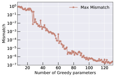
Figure 1: Largest mismatch of the surrogate (over the entire validation set) as a function of number of greedy parameters used to train the PN surrogate. The PN surrogate is seen to converge to the validation waveforms as the size of the training data set increases.

Figure 1 shows how the maximum validation error decreases as we add greedy parameters to our training data set. For our case, we stop at 100 greedy parameters (at which point the mismatch is $<10^{-6}$) and use those parameters to perform the NR simulations. Note that we don’t expect 100 NR simulations to produce an NR surrogate with comparable accuracy, $\mathcal{MM}<10^{-6}$, for two reasons. First, unlike the PN waveforms used here, the NR simulations also include the merger-ringdown part, which we expect to be more difficult to model. Second, the NR numerical truncation error is typically higher than $10^{-6}$ in mismatch, therefore the numerical noise will limit the accuracy.

III NR simulations

The NR simulations for this model are performed using the Spectral Einstein Code (SpEC) SpE ; Pfeiffer et al. (2003); Lovelace et al. (2008); Lindblom et al. (2006); Szilágyi et al. (2009); Scheel et al. (2009) developed by the SXS SXS collaboration. Of the 100 cases determined in Sec. II, only 91 simulations were successfully completed. These simulations have been assigned the identifiers SXS:BBH:1419 - SXS:BBH:1509, and are made publicly available through the SXS public catalog SXS Collaboration . For cases with equal mass, but unequal spins, we can exchange the two BHs to get an extra data point. There are 13 such cases, leading to a total of 104 NR waveforms. These are shown as circular markers in Fig. 2.

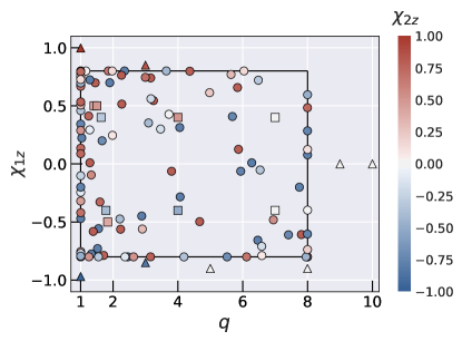
Figure 2: The parameter space covered by the 104 NR waveforms (circle markers) used in the construction of the surrogate model in Sec. VI. We also show the 9 long NR waveforms (square markers) used to test hybridization in Sec. VII.2, and the 8 NR waveforms (triangle markers) used to test extrapolation in Sec. VII.3. The axes show the mass ratio and the spin on the heavier BH, while the colors indicate the spin on the lighter BH. The black rectangle indicates the bounds of the training region: $1\leq q\leq 8$, $-0.8\leq\chi_{1z},\chi_{2z}\leq 0.8$.

The start time of these simulations varies between $4270M$ and $5227M$ before the peak of the waveform amplitude (defined in Eq. (38)), where $M=m_{1}+m_{2}$ is the total Christodoulou mass measured after the initial burst of junk radiation. The algorithm for choosing a fiducial time at which junk radiation ends is discussed in Ref. Boyle et al. (2019). The initial orbital parameters are chosen through an iterative procedure Buonanno et al. (2011) such that the orbits are quasicircular; the largest eccentricity for these simulations is $7.5\times 10^{-4}$, while the median value is $4.2\times 10^{-4}$. The waveforms are extracted at several extraction surfaces at varying finite radii form the origin and then extrapolated to future null infinity Boyle and Mroué (2009). Finally, the extrapolated waveforms are corrected to account for the initial drift of the center of mass Boyle (2016, a). The time steps during the simulations are chosen nonuniformly using an adaptive time-stepper Boyle et al. (2019). We interpolate these data to a uniform time step of $0.1M$; this is dense enough to capture all frequencies of interest, including near merger.

IV Early inspiral waveforms

While NR provides accurate waveforms, computational constraints limit NR to only the late inspiral, merger, and ringdown phases. Fortunately, PN/EOB waveforms are expected to be accurate in the early inspiral. Hence we can “stitch” together an early inspiral waveform and an NR waveform, to get a hybrid waveform Santamaría et al. (2010); Ohme (2012); Ohme et al. (2011); MacDonald et al. (2011, 2013); Ajith et al. (2012); Varma et al. (2014); Boyle (2011); Bustillo et al. (2015) that spans the entire frequency range relevant for ground-based detectors. In this section, we describe the waveforms we use for the early inspiral, leaving the hybridization procedure for the next section.

IV.1 PN waveforms

We first generate PN waveforms as implemented in the GWFrames package Boyle (b). For the orbital phase we include nonspinning terms up to 4 PN order Blanchet et al. (2004); Blanchet (2014); Jaranowski and Schäfer (2013); Bini and Damour (2013, 2014) and spin terms up to 2.5 PN order Kidder (1995); Will and Wiseman (1996); Bohe et al. (2013). We use the TaylorT4 Boyle et al. (2007) approximant to generate the PN phase; however, as described below, we replace this phase with an EOB-derived phase. For the amplitudes, we include terms up to 3.5 PN order Blanchet et al. (2008); Faye et al. (2012, 2015).

The spherical harmonic modes of the PN waveform can be written (after rescaling to unit total mass and unit distance) as Blanchet et al. (2008); Blanchet (2014),

$$\mathpzc{h}_{\ell m}^{\mathrm{PN}}=2~{}\eta~{}(v^{\mathrm{PN}})^{2}~{}\sqrt{\frac{16\pi}{5}}H_{\ell m}^{\mathrm{PN}}e^{-\mathrm{i}m\phi_{\mathrm{orb}}^{\mathrm{PN}}},$$ (4)

where $\eta=q/(1+q)^{2}$ is the symmetric mass ratio, $v^{\mathrm{PN}}$ is the characteristic speed that sets the perturbation scale in PN, $\phi^{\mathrm{PN}}_{\mathrm{orb}}$ is the (real) orbital phase, and $H_{\ell m}^{\mathrm{PN}}$ are the complex amplitudes of different modes. Note that we ignore the tail distortions Blanchet and Schäfer (1993); Arun et al. (2004) to the orbital phase as these are 4 PN corrections (see e.g. Barkett et al. (2018)).

The complex strain $\mathpzc{h}_{\ell m}^{\mathrm{PN}}$ is obtained as a time series from GWFrames. We can absorb the complex part of the amplitudes into the phases and rewrite the strain as

$$\mathpzc{h}_{\ell m}^{\mathrm{PN}}=A_{\ell m}^{\mathrm{PN}}e^{-\mathrm{i}\phi_{\ell m}^{\mathrm{PN}}},$$ (5)

$$\phi_{\ell m}^{\mathrm{PN}}=m~{}\phi_{\mathrm{orb}}^{\mathrm{PN}}+\xi^{\mathrm{PN}}_{\ell m},$$ (6)

$$\phi_{\mathrm{orb}}^{\mathrm{PN}}=\frac{\phi_{22}^{\mathrm{PN}}}{2},$$ (7)

where $A_{\ell m}^{\mathrm{PN}}$ and $\phi_{\ell m}^{\mathrm{PN}}$ are the real amplitude and phase of a given mode, and $\xi^{\mathrm{PN}}_{\ell m}$ is an offset that captures the complex part of $H_{\ell m}^{\mathrm{PN}}$. Note that Eqs. (6) and (7) together imply $\xi^{\mathrm{PN}}_{22}=0$; $H_{22}^{\mathrm{PN}}$ contains complex terms starting at 2.5PN, but these appear as 5PN corrections in the phase (see e.g. Barkett et al. (2018)), which we can safely ignore.

At this stage, $A_{\ell m}^{\mathrm{PN}}$, $\phi_{\ell m}^{\mathrm{PN}}$, and $\xi^{\mathrm{PN}}_{\ell m}$ are functions of time. But they can be recast as functions of the characteristic speed by first computing

$$v^{\mathrm{PN}}(t)=\left(\frac{d\phi^{\mathrm{PN}}_{\mathrm{orb}}}{dt}\right)^{1/3},$$ (8)

where the derivative is performed numerically, and then inverting Eq. (8) to obtain $t(v^{\mathrm{PN}})$. Then we define

$$A_{\ell m}^{\mathrm{PN}}(v^{\mathrm{PN}})=|\mathpzc{h}_{\ell m}^{\mathrm{PN}}(t(v^{\mathrm{PN}}))|,$$ (9)

$$\xi^{\mathrm{PN}}_{\ell m}(v^{\mathrm{PN}})=\phi_{\ell m}^{\mathrm{PN}}(t(v^{\mathrm{PN}}))-m~{}\phi_{\mathrm{orb}}^{\mathrm{PN}}(t(v^{\mathrm{PN}})).$$ (10)

Note that the PN waveform is generated in the source frame defined such that the reference time is the initial time. This also ensures that the heavier BH is on the positive $x-$axis at the initial time, and the initial orbital phase is zero.

To summarize: From the GWFrames package, we obtain the complex time series $\mathpzc{h}^{\mathrm{PN}}_{\ell m}$ (Eq. (5)). We compute the orbital phase (Eq. (7)), the real amplitudes (Eq. (9)), and the phase offsets (Eq. (10)). These three quantities are obtained as a time series but can be represented as functions of the characteristic speed using Eq. (8).

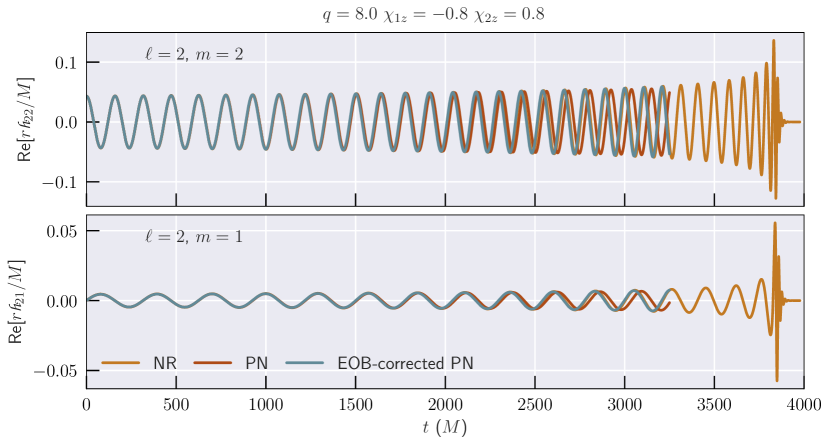
Figure 3: NR, PN (Sec. IV.1), and EOB-corrected PN (Sec. IV.2) waveforms for an example case. We show the $(2,2)$ and $(2,1)$ modes. The binary parameters are shown at the top of the plot. The EOB-corrected PN waveform Varma et al. (2014); Varma and Ajith (2017) stays faithful to the NR waveform until much later times, compared to the pure PN waveform.

IV.2 EOB correction

As was shown in previous works Varma et al. (2014); Varma and Ajith (2017), we find that the accuracy of the inspiral waveform can be improved by replacing the PN phase with the phase derived from an NR-calibrated EOB model. For this work we use SEOBNRv4 Bohé et al. (2017).

SEOBNRv4 is a time domain model that includes only the $(2,2)$ mode, which we can decompose as follows:

$$\mathpzc{h}^{\mathrm{EOB}}_{22}=A^{\mathrm{EOB}}_{22}~{}e^{-\mathrm{i}\phi^{\mathrm{EOB}}_{22}},$$ (11)

where $A^{\mathrm{EOB}}_{22}$ and $\phi^{\mathrm{EOB}}_{22}$ are the real amplitude and phase of the $(2,2)$ mode. These are functions of time, but following the same procedure as earlier, they can be recast in terms of the characteristic speed:

$$\phi^{\mathrm{EOB}}_{\mathrm{orb}}(t)=\frac{\phi^{\mathrm{EOB}}_{22}(t)}{2},$$ (12)

$$v^{\mathrm{EOB}}(t)=\left(\frac{d\phi^{\mathrm{EOB}}_{\mathrm{orb}}}{dt}\right)^{1/3},$$ (13)

where the derivative is performed numerically, and we invert Eq. (13) to obtain $t(v^{\mathrm{EOB}})$. We replace $v^{\mathrm{PN}}\rightarrow v^{\mathrm{EOB}}$ in Eqs. (9) and (10) to get, respectively, the EOB-corrected amplitudes and phase offsets:

$$A_{\ell m}^{\mathrm{ins}}(t)=A_{\ell m}^{\mathrm{PN}}(v^{\mathrm{EOB}}(t)),$$ (14)

$$\xi^{\mathrm{ins}}_{\ell m}(t)=\xi^{\mathrm{PN}}_{\ell m}(v^{\mathrm{EOB}}(t)).$$ (15)

Note that in practice, computing $A_{\ell m}^{\mathrm{ins}}(t)$ and $\xi^{\mathrm{ins}}_{\ell m}(t)$ is accomplished via an interpolation in $v$: $A_{\ell m}^{\mathrm{PN}}(v)$ and $\xi^{\mathrm{PN}}_{\ell m}(v)$ as computed in Eqs. (9) and (10) are known only at particular values of $v$, which are $v^{\mathrm{PN}}(t_{i_{\mathrm{PN}}})$ where $t_{i_{\mathrm{PN}}}$ are the times in the PN time series; we interpolate $A_{\ell m}^{\mathrm{PN}}(v)$ and $\xi^{\mathrm{PN}}_{\ell m}(v)$ to the points $v^{\mathrm{EOB}}(t_{i_{\mathrm{EOB}}})$ where $t_{i_{\mathrm{EOB}}}$ are the times in the EOB time series. We use a cubic-spline interpolation scheme as implemented in Scipy Jones et al. (2001–).

Following Eq. (6), the EOB-corrected phases are given by:

$$\phi_{\ell m}^{\mathrm{ins}}=m~{}\phi_{\mathrm{orb}}^{\mathrm{EOB}}+\xi^{\mathrm{ins}}_{\ell m},$$ (16)

where we use the EOB orbital phase from Eq. (12). Finally, our EOB-corrected inspiral waveform modes are given by:

$$\mathpzc{h}_{\ell m}^{\mathrm{ins}}=A_{\ell m}^{\mathrm{ins}}~{}e^{-\mathrm{i}\phi_{\ell m}^{\mathrm{ins}}}.$$ (17)

Fig. 3 shows an example of PN and EOB-corrected waveforms along with the corresponding NR waveform. All three waveforms have the same starting orbital frequency and their initial orbital phase is set to zero. We see that the PN waveform becomes inaccurate at late times, as expected. The EOB-corrected waveform, on the other hand, remains faithful to the NR waveform until much later times.

V Hybridization

In this section we describe our procedure to “stitch” together an inspiral waveform (described in Sec. IV) to an NR waveform (described in Sec. III).

We start by generating inspiral and NR waveforms with the same component masses and spins. We note that the spins measured in SpEC simulations agree well with PN theory Ossokine et al. (2015). However, the PN and NR waveforms are typically represented in different coordinate systems that need to be aligned with each other as follows. The two coordinate systems are related to each other by a possible time translation and a possible rotation by three Euler angles: inclination angle $\iota$, initial binary phase $\varphi_{0}$, and polarization angle $\psi$. For nonprecessing BBH the first angle $\iota$, is trivially specified by requiring that the z-axis is along the direction of orbital angular momentum. This leaves us with the freedom to vary $\varphi_{0}$ and $\psi$. We choose the hybridization frame and time shifts by minimizing a cost function in a suitable matching region; this is described in more detail below.

V.1 Choice of cost function

We use the following cost function when comparing two waveforms, $\mathpzc{h}$ and $\mathpzc{\tilde{h}}$, in the matching region:

$$\mathcal{E}[\mathpzc{h},\mathpzc{\tilde{h}}]=\frac{1}{2}\frac{\sum_{\ell,m}\int_{t_{1}}^{t_{2}}|\mathpzc{h}_{\ell m}(t)-\mathpzc{\tilde{h}}_{\ell m}(t)|^{2}dt}{\sum_{\ell,m}\int_{t_{1}}^{t_{2}}|\mathpzc{h}_{lm}(t)|^{2}dt},$$ (18)

where $t_{1}$ and $t_{2}$ denote the start and end of the matching region, to be defined in Sec. V.3, and the sum does not include $m=0$ modes for reasons described in Sec. V.2. This cost function was introduced in Ref. Blackman et al. (2017a) and is shown to be related to the weighted average of the mismatch over the sky.

We minimize the cost function by varying the time and frame shifts between the NR and inspiral waveforms

$$\min_{t_{0},\varphi_{0},\psi}\mathcal{E}[\mathpzc{h}^{\mathrm{NR}}(t;\varphi_{0},\psi),\mathpzc{h}^{\mathrm{ins}}(t;t_{0})],$$ (19)

$$\mathpzc{h}_{\ell m}^{\mathrm{NR}}(t;\varphi_{0},\psi)=\mathpzc{h}_{\ell m}^{\mathrm{NR}}(t)~{}e^{\mathrm{i}m\varphi_{0}}~{}e^{2\mathrm{i}\psi},$$ (20)

$$\mathpzc{h}_{\ell m}^{\mathrm{ins}}(t;t_{0})=\mathpzc{h}_{\ell m}^{\mathrm{ins}}(t-t_{0}).$$ (21)

We perform the time shifts on the inspiral waveform so that the matching region always corresponds to the same segment of the NR waveform. The frame shifts are performed on the NR waveform so as to preserve the initial frame alignment of the inspiral waveform (cf. Sec. IV.1). This alignment gets inherited by the hybrid waveform, and is important in the surrogate construction.

V.2 $m=0$ modes

We find that the $m=0$ modes of the inspiral waveforms do not agree very well with the NR waveforms. There are several possible reasons for this Favata (2010): (1) The NR waveform does not have the correct “memory” contribution since this depends on the entire history of the system starting at $t=-\infty$, while the NR simulation covers only the last few orbits. (2) The extrapolation to future null infinity does not work as well for these modes Boyle et al. (2019). This could be improved in the future with Cauchy Characteristic Extraction (CCE) Handmer et al. (2015, 2016); Winicour (2009); Bishop et al. (1996). (3) The amplitude of these modes is very small except very close to merger; therefore the early part of the NR waveform where we compare with the inspiral waveforms is contaminated by numerical noise.

Therefore, when constructing the hybrid waveforms, we set the entire inspiral waveform to zero for these modes,

$$\mathpzc{h}^{ins}_{\ell,m=0}=0\,.$$ (22)

When computing the cost function (Eq. (18)), we ignore the $m=0$ modes.

This means that our hybrid waveforms for these modes are equivalent to the NR waveforms. In addition, the main contribution for these modes comes from the region close to merger, which does not correspond to a memory signal, but instead is due to axisymmetric excitations near merger (cf. bottom panel of Fig. 5).

V.3 Choice of matching region

There are several considerations to take into account when choosing a matching region $[t_{1},t_{2}]$ for the cost function (Eq. (18)): (1) The NR and inspiral waveforms should agree with each other reasonably in this region; at early times the NR waveform is contaminated by junk radiation while at late times the inspiral waveform deviates from NR (cf. Figs. 3 and 5). (2) The matching region should be wide enough that the cost function is meaningful.

Our matching region starts at $1000M$ after the start of the NR waveform; we find that this is necessary to avoid noise due to junk radiation in some of the higher order modes. The length of the NR waveforms from the start of the matching region to the peak of the waveform amplitude varies between $3270M$ and $4227M$. The width of the matching region is then chosen to be equal to the time taken for 3 orbits of the binary. We use the phase of the (2,2) mode of the NR waveform to determine this. This choice ensures the width of the matching region scales appropriately with the NR starting frequency, so that we get wider matching regions when the NR waveform starts early in the inspiral.

V.4 Allowed ranges for frame and time shifts

The allowed range for $\varphi_{0}$ is [0,$2\pi$]. For nonprecessing binaries the allowed values for $\psi$ can be restricted by taking into account the symmetries of the system. We will show that this restriction is a consequence of the well-known relationship

$$\mathpzc{h}_{\ell,-m}=(-1)^{\ell}~{}\mathpzc{h}^{*}_{\ell,m}\,,$$ (23)

between the $m<0$ modes and the $m>0$ modes for nonprecessing binaries orbiting in the $x$-$y$ plane Boyle et al. (2014). We compute the shifted waveform

$$\mathpzc{h}_{\ell,-m}(t)\,e^{-\mathrm{i}m\varphi_{0}}\,e^{2\mathrm{i}\psi} =\mathpzc{h}_{\ell,-m}(t;\varphi_{0},\psi)$$

$$=(-1)^{\ell}(\mathpzc{h}_{\ell,m}(t;\varphi_{0},\psi))^{*}$$

$$=(-1)^{\ell}e^{-2\mathrm{i}\psi}e^{-\mathrm{i}m\varphi_{0}}\mathpzc{h}^{*}_{\ell,m}(t)$$

$$=e^{-2\mathrm{i}\psi}e^{-\mathrm{i}m\varphi_{0}}\mathpzc{h}_{\ell,-m}(t)$$

$$\implies e^{2i\psi}=e^{-2i\psi}.$$ (24)

Eq. (24) implies that the only allowed values for $\psi$ are $0$ and $\pi/2$ . If the inspiral waveform and the NR waveform have the same sign convention, then $\psi=0$. Unfortunately, not all NR catalogs and PN-waveform codes use the same sign convention, so we allow the possibility of $\psi=\pi/2$ to account for this.

To set the allowed range for $t_{0}$, we begin by computing the orbital frequency of the inspiral waveform, $\omega^{\mathrm{ins}}$, as half the frequency of the (2,2) mode. Similarly, we compute the orbital frequency of the NR waveform, $\omega^{\mathrm{NR}}$. We first time-align the NR and inspiral waveforms such that their frequencies match at the start of the matching region. This gives us a good starting point to vary the time shift.

We also define,

$$\omega^{\mathrm{ins}}_{\mathrm{mid}}=\omega^{\mathrm{NR}}(t=t_{1})\,,$$ (25)

$$\omega^{\mathrm{ins}}_{\mathrm{low}}=0.995\times\omega^{\mathrm{ins}}_{\mathrm{mid}}\,,$$ (26)

$$\omega^{\mathrm{ins}}_{\mathrm{hi}}=1.005\times\omega^{\mathrm{ins}}_{\mathrm{mid}}\,,$$ (27)

where $\omega^{\mathrm{NR}}(t=t_{1})$ is the NR frequency at the start of the matching region. The allowed range for time shifts $t_{0}$ is restricted to lie in the interval [$t^{\mathrm{ins}}_{\mathrm{low}}-t^{\mathrm{ins}}_{\mathrm{mid}}$, $t^{\mathrm{ins}}_{\mathrm{hi}}-t^{\mathrm{ins}}_{\mathrm{mid}}$], where $t^{\mathrm{ins}}_{\mathrm{low}}$, $t^{\mathrm{ins}}_{\mathrm{mid}}$ and $t^{\mathrm{ins}}_{\mathrm{hi}}$ are the times at which $\omega^{\mathrm{ins}}(t)$ is equal to $\omega^{\mathrm{ins}}_{\mathrm{low}}$, $\omega^{\mathrm{ins}}_{\mathrm{mid}}$ and $\omega^{\mathrm{ins}}_{\mathrm{hi}}$, respectively. In other words, the allowed range for $t_{0}$ is a region near $t_{0}=0$. $t_{0}=0$ is the case when the frequencies of the inspiral and the NR waveforms match at $t_{1}$, the start of the matching region. The lower (upper) limit for $t_{0}$ is chosen such that the inspiral waveform has a frequency equal to $0.995$ ($1.005$) times the NR frequency at $t_{1}$.

The factors in Eqs. (26) and (27) are chosen such that the time shift that minimizes the cost function is always well within the range of allowed time shifts. Hence, choosing a wider range (i.e. values of these factors farther from unity) does not improve the hybridization procedure. Note also that, like the width of the matching region in Sec. V.3, setting the range of time shifts based on the orbital frequency ensures that it scales appropriately with the start frequency of the NR waveform.

The minimization in Eq. (19) is performed as follows. We vary the time shift $t_{0}$ over 500 uniformly spaced values in the above mentioned time range . For each of these time shifts $t_{0}$, we try both allowed values of $\psi\in\{0,\pi/2\}$. For each $t_{0}$ and $\psi$, we minimize the cost function over $\varphi_{0}$ using the Nelder-Mead down-hill simplex minimization algorithm as implemented in Scipy Jones et al. (2001–). To avoid local minima in the $\varphi_{0}$ minimization, we perform 10 searches with different initial guesses, which are sampled from a uniform random distribution in the range $[0,2\pi]$.

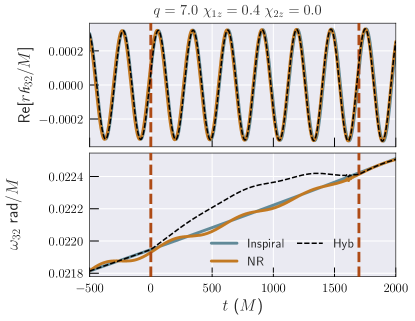
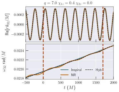
Figure 4: Left: The real part (top) and frequency (bottom) of the $(3,2)$ mode using the inertial frame stitching described in Sec. V.5.1. The binary parameters are shown on the top of the plot. The vertical red dashed lines indicate the matching region. Note that this plot shows the inspiral and NR waveforms after the time and frame shifts are performed. Right: Same, but using the amplitude-frequency stitching described in Sec. V.5.2. Now we see that the frequency of the hybrid waveform agrees much better with the NR and inspiral data.

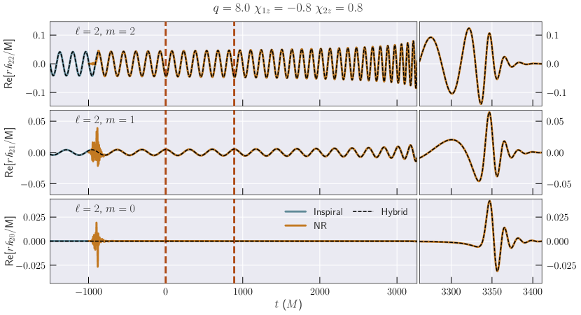
Figure 5: An example hybrid waveform used in this work. We show the $\ell=2$ modes of the inspiral, NR and hybrid waveforms. The binary parameters are shown on the top of the plot. The vertical red dashed lines indicate the matching region. Note that this plot shows the inspiral and NR waveforms after the time and frame shifts are done.

V.5 Stitching NR and inspiral waveforms.

Having obtained the right frame and time shifts between the NR and inspiral waveforms, the final step is to smoothly stitch the inspiral waveform to the shifted NR waveform. The stitching is done using a smooth blending function:

$$\tau(t)=\begin{cases}0,&\text{if}\ t<t_{1}\\ \sin^{2}\left(\frac{\pi}{2}\frac{t-t_{1}}{t_{2}-t_{1}}\right),&\text{if}\ t_{1}\leq t\leq t_{2}\\ 1,&\text{if}\ t>t_{2}\,,\end{cases}$$ (28)

where $t_{1}$ and $t_{2}$ take on the same values as those appearing in Eq. (18). Different blending functions have been proposed in the literature Ajith et al. (2008); MacDonald et al. (2011); Santamaría et al. (2010); Ajith et al. (2012). Our choice is equivalent to the blending function defined in Ref. MacDonald et al. (2011). We find that our results are not sensitive to the choice of blending function.

In what follows, for brevity, we drop the hybridization parameters $\varphi_{0}$, $\psi$, $t_{0}$ with the understanding that the models are stitched together after transforming into hybridization frame,

$$\mathpzc{h}_{\ell m}^{\mathrm{ins}}(t)\equiv\mathpzc{h}_{\ell m}^{\mathrm{ins}}(t;t_{0}),$$ (29)

$$\mathpzc{h}_{\ell m}^{\mathrm{NR}}(t)\equiv\mathpzc{h}_{\ell m}^{\mathrm{NR}}(t;\varphi_{0},\psi).$$ (30)

Given the shifted waveforms and the blending function, there are still several ways in which one can stitch the waveforms together.

V.5.1 Inertial frame stitching

One could work with the complex waveform strain and define:

$$\mathpzc{h}_{\ell m}^{\mathrm{Hyb}}=(1-\tau(t))~{}\mathpzc{h}_{\ell m}^{\mathrm{ins}}(t)+\tau(t)~{}\mathpzc{h}_{\ell m}^{\mathrm{NR}}(t)\,.$$ (31)

With this choice, by construction, the complex strain transitions smoothly from the inspiral part to the NR part over the matching region. However, the transition is more complicated for the frequency, since it involves time derivatives of the complex argument of the strain; the time derivatives of the blending function do not behave like a smooth blending function. This is demonstrated in the left panel of Fig. 4: the inspiral and NR frequencies agree well in the matching region but the frequency of the hybrid waveform deviates from this.

V.5.2 Amplitude-Frequency stitching

To avoid the undesirable artifacts described above, we choose to perform the inspiral-NR stitching using the amplitude and frequency rather than the inertial frame strain.

We begin by decomposing the NR and inspiral waveforms into their respective amplitude and phase:

$$\mathpzc{h}_{\ell m}^{\mathrm{NR}}(t)=A_{\ell m}^{\mathrm{NR}}\mathrm{e}^{-\mathrm{i}\phi_{\ell m}^{\mathrm{NR}}}\,,\quad\mathpzc{h}_{\ell m}^{\mathrm{NR}}(t)=A_{\ell m}^{\mathrm{ins}}\mathrm{e}^{-\mathrm{i}\phi_{\ell m}^{\mathrm{ins}}}\,.$$ (32)

The frequency of each mode

$$\omega_{\ell m}^{\mathrm{NR}}=\frac{d\phi_{\ell m}^{\mathrm{NR}}}{dt}\,,\qquad\omega_{\ell m}^{\mathrm{ins}}=\frac{d\phi_{\ell m}^{\mathrm{ins}}}{dt}\,,$$ (33)

is then numerically computed from 4th-order finite difference approximations to the time derivative. Finally, we stitch the amplitude and frequency of each mode to get their hybrid versions:

$$A_{\ell m}^{\mathrm{Hyb}}=(1-\tau(t))~{}A_{\ell m}^{\mathrm{ins}}(t)+\tau(t)~{}A_{\ell m}^{\mathrm{NR}},$$ (34)

$$\omega_{\ell m}^{\mathrm{Hyb}}=(1-\tau(t))~{}\omega_{\ell m}^{\mathrm{ins}}(t)\ +\tau(t)~{}\omega_{\ell m}^{\mathrm{NR}}\,.$$ (35)

To get the inertial frame strain we first need to integrate the frequency to get the phase. However, we already know the phase in the region before (only inspiral) and after (only NR) the matching region. So, we integrate the hybrid frequency

$$\phi_{\ell m}^{\mathrm{Hyb-match-region}}=\int_{t_{1}}^{t_{2}}\omega_{\ell m}^{\mathrm{Hyb}}dt\,,$$ (36)

in the matching region using a 4th-order accurate Runge-Kutta scheme.

Finally, we set the phase of the hybrid waveform to,

$$\phi_{\ell m}^{\mathrm{Hyb}}=\begin{cases}\phi_{\ell m}^{\mathrm{ins}}+\delta^{1}_{\ell m},&\text{if}\ t<t_{1}\\ \phi_{\ell m}^{\mathrm{Hyb-match-region}}+\delta^{2}_{\ell m},&\text{if}\ t_{1}\leq t\leq t_{2}\\ \phi_{\ell m}^{\mathrm{NR}},&\text{if}\ t>t_{2}\,,\end{cases}$$ (37)

where $\delta^{1}_{\ell m}$ and $\delta^{2}_{\ell m}$ are chosen such that $\phi_{\ell m}^{\mathrm{Hyb}}$ is continuous at $t_{1}$ and $t_{2}$.

Since, by construction, the frequency transitions smoothly from the inspiral-waveform to NR data, we eliminate the artifact seen in the bottom left panel of Fig 4 (dashed line), as demonstrated in the right panel of Fig. 4.

We note that since the $m=0$ modes are purely real/imaginary and nonoscillatory for nonprecessing systems, they do not have a frequency associated with them, therefore we use the inertial frame stitching of Sec. V.5.1 for these modes. For these modes the waveform goes from zero to the NR value over the matching region.

In the hybridized waveform we include the $\ell\leq 4$ and $(5,5)$ modes, but not the $(4,1)$ or $(4,0)$ modes. For the $(4,1)$ and $(4,0)$ modes we find that the inspiral and NR waveforms do not agree very well. This is possibly due to issues in the extrapolation to future-null infinity Boyle and Mroué (2009) for these modes, and could be resolved in the future with CCE Handmer et al. (2015, 2016); Winicour (2009); Bishop et al. (1996) An example of the final NR, inspiral and hybrid waveforms is shown in Fig. 5.

VI Building the surrogate model

Starting from the 104 NR waveforms described in Sec. II and Sec. III, we construct hybrid waveforms as described in Sec. V. In this section we describe our method to construct a surrogate model for these hybrid waveforms.

VI.1 Processing the training data

Before building a surrogate model, we process the hybrid waveforms as follows.

VI.1.1 Time shift

We shift the time arrays of the hybrid waveforms such that the peak of the total amplitude

$$A_{tot}=\sqrt{\sum_{l,m}|\mathpzc{h}_{\ell m}|^{2}}\,,$$ (38)

occurs at $t=0$ for each waveform.

VI.1.2 Frequency and mass ranges of validity

The length of a hybrid waveform is set by choosing a starting orbital frequency $\omega_{0}$, for the inspiral waveform; we use $\omega_{0}=2\times 10^{-4}~{}\text{rad}/M$ for all waveforms. However, for the same starting frequency, the length in time of the waveform is different for different mass ratios and spins. Since we want to construct a time-domain surrogate model, we require a common time array for all hybrid waveforms. The initial time for the surrogate is determined by the shortest hybrid waveform in the training data set; this waveform begins at a time $\sim 5.4\times 10^{8}M$ before the peak. We truncate all hybrid waveforms to this initial time value.

The largest starting orbital frequency among the truncated hybrid waveforms is $\omega_{0}=2.9\times 10^{-4}~{}\text{rad}/M$, which sets the low frequency limit of validity of the surrogate. For LIGO, assuming a starting GW frequency of $20~{}\text{Hz}$, the $(2,2)$ mode of the surrogate is valid for total masses $M\geq 0.9M_{\odot}$. The highest spin-weighted spherical harmonic mode we include in the surrogate model is $(5,5)$, for which the frequency is $5/2$ times that of the $(2,2)$ mode. Therefore, all modes of the surrogate are valid for $M\geq 2.25M_{\odot}$. This coverage of total mass is sufficient to model all stellar mass binaries of interest for ground based detectors; for an equal mass binary neutron star system, the total mass is $M\sim 2.7M_{\odot}$.

VI.1.3 Downsampling and common time samples

Because the hybrid waveforms are so long, it is not practical to sample the entire waveform with the same step size we use for the NR waveforms ($0.1M$). Fortunately, the early low-frequency portion of each waveform requires sparser sampling than the later high-frequency portion. We therefore down-sample the time arrays of the truncated hybrid waveforms to a common set of time samples. We choose these samples so that there are 5 points per orbit for the above-mentioned shortest hybrid waveform in the training data set, except for $t\geq-1000M$ we choose uniform time samples separated by $0.1M$. This ensures that we have a denser sampling rate at late times when the frequency is higher. We retain times up to $135M$, which is sufficient to capture the entire ringdown.

Before downsampling, we first transform the waveform into the co-orbital frame, defined as:

$$\mathpzc{h}_{\ell m}^{C}=\mathpzc{h}_{\ell m}~{}e^{\mathrm{i}m\phi_{\mathrm{orb}}},$$ (39)

$$\mathpzc{h}_{22}=A_{22}~{}e^{-\mathrm{i}\phi_{22}},$$ (40)

$$\phi_{\mathrm{orb}}=\frac{\phi_{22}}{2},$$ (41)

where $\mathpzc{h}_{\ell m}$ is the inertial frame hybrid waveform, $\phi_{\mathrm{orb}}$ is the orbital phase, and $\phi_{22}$ is the phase of the $(2,2)$ mode. The co-orbital frame can be thought of as roughly co-rotating with the binary, since we perform a time-dependent rotation given by the instantaneous orbital phase. Therefore the waveform is a slowly varying function of time in this frame, increasing the accuracy of interpolation to the chosen common time samples. For the $(2,2)$ mode we save the downsampled amplitude $A_{22}$ and phase $\phi_{22}$, while for all other modes we save $\mathpzc{h}_{\ell m}^{C}$. We find that this down-sampling results in interpolation errors $\mathcal{E}\lesssim 10^{-10}$ (defined in Eq. (18)) for all hybrid waveforms.

VI.1.4 Phase alignment

After down-sampling to the common temporal grid of the surrogate, we rotate the waveforms about the z-axis such that the orbital phase $\phi_{\mathrm{orb}}$ is zero at $t=-1000M$. Note that this by itself would fix the physical rotation up to a shift of $\pi$. When generating the inspiral waveforms for hybridization, we align the system such that the heavier BH is on the positive $x-$axis at the initial frequency; this fixes the $\pi$ ambiguity. Therefore, after this phase rotation, the heavier BH is on the positive $x-$axis at $t=-1000M$ for all waveforms.

VI.2 Decomposing the data

It is much easier to build a model for slowly varying functions of time. Therefore, rather than work with the inertial frame strain $\mathpzc{h}_{\ell m}$, which is oscillatory, we work with simpler “waveform data pieces” , as explained below. We build a separate surrogate for each waveform data piece. When evaluating the full surrogate model, we first evaluate the surrogate of each data piece and then recombine the data pieces to get the inertial frame strain.

A common choice in literature when working with nonprecessing waveforms has been to decompose the complex strain into an amplitude and phase, each of which is a slowly varying function of time:

$$\mathpzc{h}_{\ell m}=A_{\ell m}e^{-\mathrm{i}\phi_{\ell m}}.$$ (42)

However, when $q=1$ and $\chi_{1z}=\chi_{2z}$, the amplitude of odd-$m$ modes becomes zero due to symmetry. This means that the phase becomes meaningless, so one has to treat such cases separately. For example, Ref Blackman et al. (2015) used specialized basis functions for the odd-$m$ modes that captured the divergent behavior of the phase in the equal-mass limit.

To avoid this issue, instead of using the amplitude and phase we use the real and imaginary parts of the co-orbital frame strain $\mathpzc{h}_{\ell m}^{C}$, defined in Eq. (39), for all nonquadrupole modes. The co-orbital frame strain is always meaningful: in the special, symmetric case mentioned above, the co-orbital frame strain for the odd-$m$ modes just goes to zero, rather than diverge. For the $(2,2)$ mode we use the amplitude $A_{22}$ and phase $\phi_{22}$.

As mentioned above, our hybrid waveforms are very long, typically containing $\sim 3\times 10^{4}$ orbits. This presents new challenges that are not present for pure-NR surrogates. For instance, $\phi_{22}$ sweeps over $\sim 4\times 10^{5}$ radians for a typical hybrid waveform. We find that the accuracy of the surrogate model at early times improves if we first subtract a PN-derived approximation to the phase, model the phase difference rather than $\phi_{22}$, and then add back the PN contribution when evaluating the surrogate model. In particular, we use the leading order TaylorT3 approximant Damour et al. (2001). For this approximant, the phase is given as an analytic, closed-form, function of time. Therefore, even though TaylorT3 is known to be less accurate than some other approximants Buonanno et al. (2009), its speed makes it ideal for our purpose as we only need it to capture the general trend. At leading order, the TaylorT3 phase is given by:

$$\phi^{T3}_{22}=\phi^{T3}_{\mathrm{ref}}-\frac{2}{\eta~{}\theta^{5}},$$ (43)

where $\phi^{T3}_{\mathrm{ref}}$ is an arbitrary integration constant, $\theta=[\eta~{}(t_{\mathrm{ref}}-t)/(5M)]^{-1/8}$, $t_{\mathrm{ref}}$ is an arbitrary time offset, and $\eta$ is the symmetric mass ratio. Note that $\phi^{T3}_{22}$ diverges at $t=t_{\mathrm{ref}}$. We choose $t_{\mathrm{ref}}=1000M$, long after the end of the waveform (recall that the peak is at $t=0$), to ensure that we are always far away from this divergence. We choose $\phi^{T3}_{\mathrm{ref}}$ such that $\phi^{T3}_{22}=0$ at $t=-1000M$; this is the same time at which we align the hybrid phase in Sec. VI.1.4.

Instead of modeling $\phi_{22}$, we model the residual

$$\phi^{\mathrm{res}}_{22}=\phi_{22}-\phi^{T3}_{22}\,,$$ (44)

after removing the leading-order contribution $\phi^{T3}_{22}$. By construction, $\phi^{\mathrm{res}}_{22}$ goes to zero at $t=-1000M$. We find that after removing the leading order TaylorT3 phase, the scale of $\phi^{\mathrm{res}}_{22}$ for a typical hybrid is $\sim 10^{3}$ radians, compared to $\sim 4\times 10^{5}$ radians for $\phi_{22}$. In essence, this captures almost all of the phase evolution in the early inspiral, simplifying the problem of modeling the phase to the same as modeling the phase of late-inspiral NR waveforms. We stress that the exact form of $\phi^{T3}_{22}$ (or its physical meaning) is not important, as long as it captures the general trend, since we add the exact same $\phi^{T3}_{22}$ to our model of $\phi^{\mathrm{res}}_{22}$ when evaluating the surrogate. In fact, we find that adding higher order PN terms in Eq. (43) does not improve the accuracy of the surrogate.

To summarize, we decompose the hybrid waveforms into the following waveform data pieces, each of which is a smooth, slowly varying function of time: ($A_{22}$, $\phi^{\mathrm{res}}_{22}$) for the (2,2) mode, and the real and imaginary parts of $\mathpzc{h}_{\ell m}^{C}$ for all other modes.

VI.3 Building the surrogate

Once we have the waveform data pieces, we build a surrogate model for each data piece using the procedure outlined in Refs. Blackman et al. (2017a); Field et al. (2014), which we only briefly describe here. Note that the steps below are applied independently for each waveform data piece.

VI.3.1 Greedy basis

We first construct a greedy reduced-basis Field et al. (2011) such that the projection errors (cf. Eq. (5) of Ref. Blackman et al. (2017a)) for the entire data set onto this basis are below a given tolerance. For the basis tolerances we use $10^{-2}$ radians for the $\phi^{\mathrm{res}}_{22}$ data piece, $2\times 10^{-5}$ for $A_{22}$, and $8\times 10^{-6}$ for all other data pieces. These are chosen through visual inspection of the basis functions to ensure they are not noisy, and based on the expected truncation error of the NR waveforms. For instance, we expect the error in phase to be about $10^{-2}$ radians.

The greedy procedure is initialized with a single basis function as described in Ref. Blackman et al. (2017a). Then at each step in the greedy procedure, the waveform with the highest projection error onto the current basis is added to the basis. Previous work has shown that the resulting greedy reduced-basis is robust to different choices of initialization Herrmann et al. (2012). When computing the basis projection errors, we only include data up to $50M$ after the peak. We find that this helps avoid noisy basis functions. This is particularly important for the phase data piece as this becomes meaningless at late times, when the waveform amplitude becomes very small.

VI.3.2 Empirical interpolation

Next, using a different greedy procedure, we construct an empirical interpolant Barrault et al. (2004); Maday et al. (2009); Hesthaven, Jan S. et al. (2014) in time. This picks out the most representative time nodes, where the number of time nodes is the same as the number of greedy basis functions. We require that the start of the waveform always be included as a time node for all data pieces. This is a useful modeling choice because the magnitude of the waveform data pieces in the very early inspiral can be smaller than the basis tolerances mentioned above. By requiring the first index to be an empirical time node, we enforce an anchor point that ensures the waveform data piece has the right magnitude at the start of the waveform. Furthermore, we do not allow any empirical time nodes at times $>50M$, since we expect this part to be dominated by noise (especially for the phase data piece).

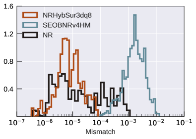
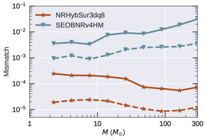
Figure 6: Errors in NRHybSur3dq8 and SEOBNRv4HM when compared against hybrid waveforms. For NRHybSur3dq8, we show out-of-sample errors. Mismatches are computed at several points in the sky of the source frame using all available modes in each waveform: For the hybrid waveforms and NRHybSur3dq8, that is $\ell\leq 4$ and $(5,5)$, but not $(4,1)$ or $(4,0)$. For SEOBNRv4HM that is $(2,2),(2,1),(3,3),(4,4)$, and $(5,5)$. Left: Mismatches computed using a flat noise curve, but including only the late inspiral part of the waveforms, starting at $-3500M$ before the peak. Therefore, we are essentially comparing only to the NR part of the hybrid waveforms. For comparison, we also show the NR resolution error, obtained by comparing the two highest available resolutions. The histograms are normalized such that the area under each curve is $1$ when integrated over $\log_{10}$(Mismatch). Right: Mismatches as a function of total mass, computed using the Advanced LIGO design sensitivity noise curve. Here we compare against the full hybrid waveforms. The solid (dashed) lines show the 95th percentile (median) mismatch values over points on the sky as well as different hybrid waveforms.

VI.3.3 Parametric fits

Finally, for each time node, we construct a fit across the parameter space. The fits are done using the Gaussian process regression (GPR) fitting method described in the supplemental material of Ref. Varma et al. (2019). Following Ref. Varma et al. (2019), we parameterize our fits using $\log(q)$, $\hat{\chi}$, and $\chi_{a}$. Here $\hat{\chi}$ is the spin parameter entering the GW phase at leading order Khan et al. (2016); Ajith (2011); Cutler and Flanagan (1994); Poisson and Will (1995) in the PN expansion,

$$\chi_{\mathrm{eff}}=\frac{q~{}\chi_{1z}+\chi_{2z}}{1+q}\,,$$ (45)

$$\hat{\chi}=\frac{\chi_{\mathrm{eff}}-38\eta(\chi_{1z}+\chi_{2z})/113}{1-{76\eta}/{113}}\,,$$ (46)

and $\chi_{a}$ is the “anti-symmetric spin”,

$$\chi_{a}=\tfrac{1}{2}(\chi_{1z}-\chi_{2z})\,.$$ (47)

The fit accuracy, and as a result the accuracy of the surrogate model, improves noticeably when using $\log(q)$, compared to $q$ or $\eta$.

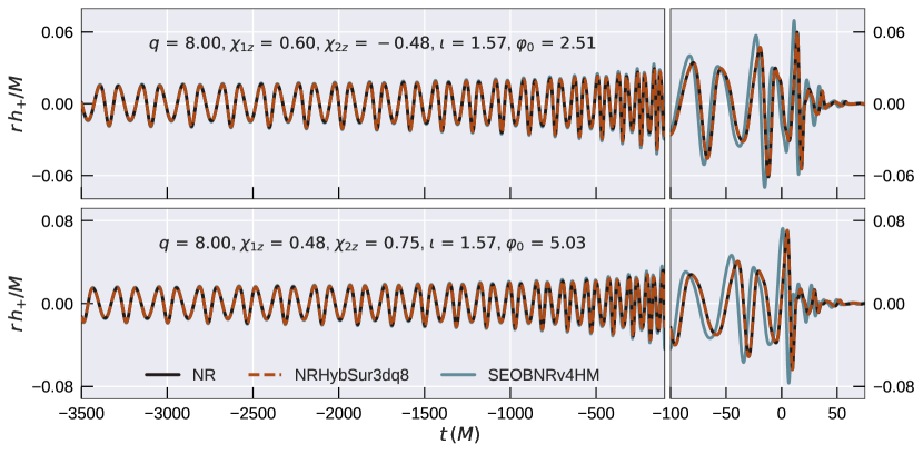
Figure 7: The plus polarization of the waveforms for the cases that result in the largest mismatch for NRHybSur3dq8 (top) and SEOBNRv4HM (bottom) in the left panel of Fig. 6. We also show the corresponding hybrid waveforms (labeled as NR because only the late part is shown). Each waveform is projected using all available modes for that model, along the direction which results in the largest mismatch for NRHybSur3dq8 (SEOBNRv4HM) in the top (bottom) panel. Note that NRHybSur3dq8 is evaluated using trial surrogates that are not trained using these cases. The binary parameters and the direction in the source frame are indicated in the inset text. All waveforms are time shifted such that the peak of the total waveform amplitude occurs at $t=0$ (using all available modes, according to Eq. (38)). Then the waveform modes are rotated about the $z-$axis such that the orbital phase is zero at $t=-3500M$.

VI.4 Evaluating the surrogate

When evaluating the surrogate waveform, we first evaluate each surrogate waveform data piece. Next, we compute the phase of the $(2,2)$ mode,

$$\phi^{\mathrm{S}}_{22}\equiv\phi^{\mathrm{res,S}}_{22}+\phi^{T3}_{22},$$ (48)

where $\phi^{\mathrm{res,S}}_{22}\approx\phi^{\mathrm{res}}_{22}$ is the surrogate model for $\phi^{\mathrm{res}}_{22}$ and $\phi^{T3}_{22}$ is given in Eq. (43). If the waveform is required at a uniform sampling rate, we interpolate each waveform data piece from the sparse time samples used to construct the model to the required time samples, using a cubic-spline interpolation scheme. Finally, we use Eqs. (39), (40), and (41) to reconstruct the surrogate prediction for the inertial frame strain.

VII Results

In order to estimate the difference between two waveforms, $\mathpzc{h}_{1}$ and $\mathpzc{h}_{2}$, we use the mismatch, defined in Eq. (2), but in this section instead of Eq. (3) we use the frequency-domain inner product

$$\left<\mathpzc{h}_{1},\mathpzc{h}_{2}\right>=4\mathrm{Re}\int_{f_{\mathrm{min}}}^{f_{\mathrm{max}}}\frac{\tilde{\mathpzc{h}}_{1}(f)\tilde{\mathpzc{h}}_{2}^{*}(f)}{S_{n}(f)}df,$$ (49)

where $\tilde{\mathpzc{h}}(f)$ indicates the Fourier transform of the complex strain $\mathpzc{h}(t)$, $*$ indicates a complex conjugation, $\mathrm{Re}$ indicates the real part, and $S_{n}(f)$ is the one-sided power spectral density of a GW detector. We taper the time domain waveform using a Planck window McKechan et al. (2010), and then zero-pad to the nearest power of two. We further zero-pad the waveform to increase the length by a factor of eight before performing the Fourier transform. The tapering at the start of the waveform is done over $1.5$ cycles of the $(2,2)$ mode. The tapering at the end is done over the last $20M$. Note that our model contains times up to $135M$ after the peak of the waveform amplitude, and the signal has essentially died down by the last $20M$.

We compute mismatches following the procedure described in Appendix D of Ref. Blackman et al. (2017a): the mismatches are optimized over shifts in time, polarization angle, and initial orbital phase. Both plus and cross polarizations are treated on an equal footing by using a two-detector setup where one detector sees only the plus and the other only the cross polarization. We compute the mismatches at 37 points uniformly distributed on the sky in the source frame, and we use all available modes of a given waveform model.

When computing flat noise mismatches ($S_{n}=1$), we take $f_{\mathrm{min}}$ to be the frequency of the $(2,2)$ mode at the end of the initial tapering window, and $f_{\mathrm{max}}=5f^{peak}_{22}$, where $f^{peak}_{22}$ is the frequency of the $(2,2)$ mode at its peak. This choice of $f_{\mathrm{max}}$ ensures that we capture the peak frequencies of all modes considered in this work, including the $(5,5)$ mode, whose frequency has the highest multiple of the $(2,2)$ mode frequency of all the modes we model. We also compute mismatches with the Advanced-LIGO design sensitivity Zero-Detuned-HighP noise curve LIGO Scientific Collaboration (2011) with $f_{\mathrm{min}}=20\text{Hz}$ and $f_{\mathrm{max}}=2000\text{Hz}$.

VII.1 Surrogate errors

We evaluate the accuracy of our new surrogate model, NRHybSur3dq8, by computing mismatches against hybrid waveforms. For this, we compute “out-of-sample” errors as follows. We first randomly divide the 104 training waveforms into groups of $\mathchar 21016\relax 5$ waveforms each. For each group, we build a trial surrogate using the remaining $\mathchar 21016\relax 99$ training waveforms and test against these five validation ones. We also compute the mismatch between an existing higher-mode waveform model, SEOBNRv4HM Cotesta et al. (2018), and the hybrid waveforms.

Figure 6 summarizes mismatches of both NRHybSur3dq8 and SEOBNRv4HM versus the hybrid waveforms. We use all available modes for each waveform model. In the left panel we show mismatches computed using a flat noise curve over the NR part of the hybrid waveforms (to do this, we truncate the waveforms and begin tapering at $t=-3500M$). We see that the mismatches for NRHybSur3dq8 are about two orders of magnitude lower than that of SEOBNRv4HM. We compare this with the truncation error in the NR waveforms themselves, by computing the mismatch between the two highest available resolutions of each NR waveform. The errors in the surrogate model are well within the truncation error of the NR simulations. Note that NR error estimated in this manner is a conservative estimate; if we treat the high resolution simulation as the fiducial case, the NR curve in Fig. 6 can be thought of as the error in the lower-resolution simulation. This explains why the errors in the surrogate are smaller than the NR errors. We suspect that the error of the high resolution simulations is close to the surrogate model’s error.

The right panel of Fig. 6 shows mismatches computed using the Advanced LIGO design sensitivity noise curve. The mismatches are now dependent on the total mass of the system, so we show mismatches for masses starting at the lower limit of the range of validity of the surrogate: $M\geq 2.25M_{\odot}$. 95th percentile mismatches for NRHybSur3dq8, are always below $\mathchar 21016\relax 3\times 10^{-4}$ in the mass range $2.25M_{\odot}\leq M\leq 300M_{\odot}$. At high masses ($M\gtrsim 40M_{\odot}$), where the merger and ringdown are more prominent, our model is more accurate than SEOBNRv4HM by roughly two orders of magnitude, in agreement with the left panel of Fig. 6.

For high masses only the last few orbits of the hybrid waveforms are in the LIGO band, and the hybrid waveforms are effectively the same as the NR waveforms. For low masses, the errors in the right panel of Fig. 6 quantify how well different models reproduce the hybrid waveforms. However, this comparison cannot account for the errors in the hybridization procedure itself. We provide some evidence for the fidelity of the hybrid waveforms in Sec. VII.2, by comparing against some long NR waveforms.

Fig. 7 shows NRHybSur3dq8 and SEOBNRv4HM waveforms for the cases leading to the largest errors in the left panel of Fig. 6. The surrogate shows very good agreement with the NR waveform, even for its worst case. SEOBNRv4HM shows a noticeably larger deviation that cannot all be accounted for with a time and/or phase shift. Note that we align the time and orbital phase of the waveforms in Fig. 7.

We note that the main improvement over SEOBNRv4HM is not due to the inclusion of more modes. We find that the agreement between SEOBNRv4HM and the NR/hybrid waveforms in Figs. 6 and 7 improves only marginally when restricting the NR/hybrid waveforms to the same set of modes as SEOBNRv4HM.

VII.2 Hybridization errors

The errors described in Sec. VII.1 are computed by comparing the surrogate against hybrid waveforms, hence they do not include the errors in the hybridization procedure or the errors from EOB-corrected-PN waveforms (cf. Sec. IV.2) we use for the early inspiral. To estimate these errors, we compare the surrogate against a few very long NR simulations . We perform five new simulations that are $\sim 10^{5}M$ long and two that are $\sim 3\times 10^{4}M$ long. These have been assigned the identifiers SXS:BBH:1412 - SXS:BBH:1418, and will be made publicly available in the upcoming update of the SXS public catalog SXS Collaboration . In addition, we use two simulations of length $\sim 3\times 10^{4}M$ from Ref. Kumar et al. (2015). These nine simulations are represented as square markers in Fig. 2, and have not been used in training the surrogate. The surrogate was trained against hybrid waveforms whose NR duration varied between $3270M$ and $4227M$. Therefore, comparing against long NR waveforms, which include the early inspiral, is a good way to estimate the hybridization error.

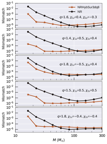
Figure 8: Comparisons between the NRHybSur3dq8 surrogate model and a few NR waveforms of $\mathchar 21016\relax 10^{5}M$ in duration. We also show the NR resolution error. 95th percentile mismatches (over points in the sky) are shown as a function of total mass. The inset text indicates the mass ratio and component spins. Mismatches are computed using the Advanced LIGO design sensitivity noise curve. To best assess the error introduced by the hybridization procedure we use the same set of modes for the NR waveforms as the surrogate. At low masses, the hybridization errors (red circles) become less reliable measures of accuracy due to the large NR resolution error (black circles) itself. Fig. 9 describes a refined comparison to improve the assessment at low masses.

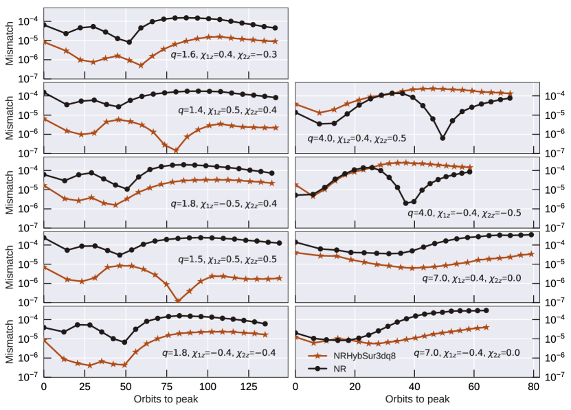
Figure 9: Errors in the NRHybSur3dq8 surrogate model against long NR waveforms, but only looking at segments of length $\Delta t=5\times 10^{3}M$ individually. Each point represents one segment that ends at a specified number of orbits before the waveform peak, as plotted on the horizontal axis; Therefore, going from left to right in the figure, we plot segments that start earlier in the inspiral. We also show the NR resolution error in the same segments. The inset text indicates the mass ratio and component spins. We show 95th percentile mismatches (over points in the sky), computed using a flat noise curve. We use the same set of modes for the NR waveforms as the surrogate. We find that, in general, the surrogate error is lower than or comparable to the NR resolution error throughout the inspiral.

We begin by repeating the mismatch computation from the right panel of Fig. 6, using the $10^{5}M$ long NR waveforms. This is shown in Fig. 8. We also show the errors in the NR simulations, estimated by comparing the two highest available NR resolutions. We find that the mismatches between the surrogate and the long NR waveforms for $M>30M_{\odot}$ are below $10^{-4}$, in agreement with Fig. 6. For lower masses, the mismatches quickly increase and can be as high as $\sim 10^{-2}$. However, this increase in mismatch is accompanied by an increase in the error of the NR waveforms. This is expected, since for very long NR waveforms the accumulated phase error is a dominant source of numerical error, which becomes increasingly relevant for low mass systems as more of the waveform moves in-band. Therefore, in Fig. 8, at low masses, the comparison between the surrogate and NR waveforms is largely dominated by the numerical resolution error of the long NR waveforms themselves.

We find that a better test of the hybridization procedure, one that is less sensitive to NR phase accumulation errors, is to compare against different segments of the NR waveform. Since the phase errors accumulate over a large number of cycles, by looking at smaller segments we ensure that this contribution is not the dominant error. To be precise, we compare the surrogate and the NR data, using segments of length $\Delta t=5\times 10^{3}M$ ending at a particular number of orbits before the peak of the waveform. For each segment we compute mismatches at several points in the sky using a flat noise curve. By varying the number of orbits to the peak, we can cover the entire NR waveform including the early inspiral region where the surrogate depends on the hybridization procedure. These errors are shown in Fig. 9. We find that in each segment, the mismatch between the surrogate and the NR data is, in general, lower or comparable to the NR resolution error. Therefore, the surrogate reproduces the NR data accurately in the early inspiral and the hybridization errors are smaller than or comparable to the NR resolution error for these cases. We note that the surrogate errors in Fig. 9 depend on the length of the segment considered and are only meaningful when compared to the NR errors in the same segment.

Unfortunately, long NR simulations such as these are not available at regions of the parameter space where both mass ratio and spin magnitudes are large. These are the cases where PN is expected to perform poorly, so we expect larger hybridization errors for these cases.

VII.3 Extrapolation outside the training range

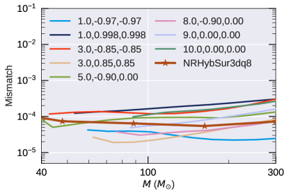
Figure 10: Errors in NRHybSur3dq8 when evaluated outside its training range. 95th percentile mismatches (over points in the sky) are shown as a function of total mass for different extrapolated cases. These are computed using the Advanced LIGO design sensitivity noise curve. To best assess the error introduced by the extrapolation, we use the same set of modes for the NR waveforms as the surrogate. The labels indicate the mass ratio and component spins ($q,\chi_{1z},\chi_{2z}$). For comparison we reproduce the 95th percentile mismatches for NRHybSur3dq8 within its training range from the right panel of Fig. 6.

We now investigate the efficacy of NRHybSur3dq8 to extrapolate beyond its training parameter range by comparing against SpEC NR simulations SXS Collaboration ; Kumar et al. (2015); Chu et al. (2016); Scheel et al. (2015); Chatziioannou et al. (2018) at larger mass ratios ($8<q\leq 10$) and/or larger spin magnitudes ($|\chi_{1z}|>0.8$ or $|\chi_{12}|>0.8$). These NR simulations are represented as triangle markers in Fig. 2.

Fig. 10 shows mismatches for NRHybSur3dq8 when compared against these simulations. We find that surrogate extrapolates remarkably well, with the mismatch always $\lesssim 4\times 10^{-4}$ for all cases, which include mass ratios up to $q=10$ and spin magnitudes up to $|\chi|=0.998$. However, the extrapolation errors can be about half an order of magnitude larger than errors within the training range. Note that NR simulations with both high mass ratios and high spin magnitudes are not currently available, and the ones used here represent the most extreme cases found in the SXS Catalog. We do not hybridize these simulations before comparing to NRHybSur3dq8 because several of them are too short. In Fig. 10, the minimum mass for each case is chosen to be the lowest mass at which all used modes of the NR simulation lie fully in the LIGO band with a low frequency cut-off of $20~{}\text{Hz}$.

At much higher mass ratios than those tested here, such as $q=15$, we find that the waveforms generated by the surrogate can have “glitches” in the time series. Therefore, we recommend the surrogate be used for $q\leq 10$ and $|\chi_{1z}|,|\chi_{2z}|\leq 1$. However, we advise caution with any extrapolation in general.

VII.4 Mode mixing

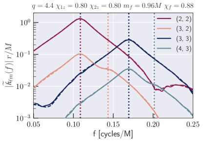
Figure 11: Mode mixing between spherical harmonic modes is clearly seen in the ringdown signal of the NR waveform and is accurately reproduced by the surrogate. The absolute values of the Fourier transform of different spherical harmonic modes are shown as solid (dashed) curves for the surrogate (NR). The dotted vertical lines indicate the frequencies of the fundamental QNM overtone of these modes. The component parameters as well as the remnant mass and spin are shown in the text above the figure.

Numerical relativity waveforms are extracted as spin-weighted spherical harmonic modes Newman and Penrose (1966); Goldberg et al. (1967). However, in the ringdown regime, the natural basis to use is the spin-weighted spheroidal harmonic basis Teukolsky (1973, 1972). A spherical harmonic mode $\mathpzc{h}_{\ell m}$ can be written as a linear combination of all spheroidal harmonic modes $\mathpzc{h}_{\ell m}^{S}$ with the same $m$ index Berti and Klein (2014). Therefore, during the ringdown, we expect leakage of power between different spherical harmonic modes with the same $m$. This is referred to as mode mixing.

Since the surrogate accurately reproduces the spherical harmonic modes from the NR simulations, it also captures this mode mixing. We demonstrate this for an example case in Fig. 11. Here we compute the Fourier transform of different spherical harmonic modes in the ringdown stage of the waveform. Before computing the Fourier transform, we first drop all data before $t=20M$, where $t=0$ corresponds to the peak of the waveform amplitude (cf. Eq. (38)). Then, we taper the data between $t=20M$ and $t=40M$, as well as the last $10M$ of the time series, using a Planck window McKechan et al. (2010). The tapering width at the start is chosen such that the remaining signal is dominated by the fundamental quasi-normal mode (QNM) overtone. Fig. 11 shows the absolute value of these Fourier transforms for different modes, for both the surrogate and the NR waveform. In addition, we show the frequency of the fundamental QNM overtone for each mode Berti and Klein .

Note that the $(2,2)$ mode and the $(3,2)$ mode have the same $m$ index, the condition required for mode mixing. We see that the peak of the $(2,2)$ mode agrees with the QNM frequency as expected. For the $(3,2)$ mode however, while there are features of a peak at the expected QNM frequency, there is a much larger peak at the frequency of the $(2,2)$ mode. This is because some of the power of the stronger $(2,2)$ mode has leaked into the $(3,2)$ mode due to mode mixing. Mode mixing can also be seen for the $(3,3)$ and $(4,3)$ modes, which also have the same $m$ index. Fig. 11 shows that not only does the surrogate agree with NR in the ringdown, it also reproduces the mode mixing present in the NR data.

VII.5 Evaluation cost

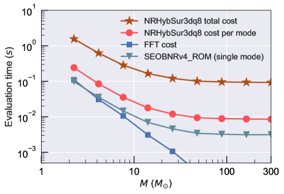
Figure 12: Evaluation cost for NRHybSur3dq8 including the cost of an FFT. We show the cost for evaluating all 11 modes modeled by NRHybSur3dq8, as well as the cost per mode. The FFT cost is included in both of the above but also shown separately. We also show the evaluation cost of SEOBNRv4_ROM which includes only the $(2,2)$ mode. The evaluation cost is computed by averaging over 64 points uniformly distributed in the parameter space, $q\leq 8$ and $|\chi_{1z}|,|\chi_{2z}|\leq 0.8$.

Figure 12 shows the evaluation cost for NRHybSur3dq8, at different total masses, starting at $20\text{Hz}$, and using a sampling rate of $4096\text{Hz}$. This suggests that NRHybSur3dq8 is fast enough for direct use in parameter estimation. We also show the evaluation cost per mode. Note that the total cost as well the cost per mode in Fig. 12 include the cost of a Fast Fourier Transform (FFT). We perform the FFT only once, after summing over all modes in the time domain. This cost is also shown separately in Fig. 12. Finally, we show the evaluation cost of SEOBNRv4_ROM Bohé et al. (2017), a Fourier domain Reduced Order Model (ROM) version of SEOBNRv4. Note that SEOBNRv4_ROM models only the $(2,2)$ mode. Comparing the cost for SEOBNRv4_ROM to the cost per mode of NRHybSur3dq8 suggests that the evaluation cost of NRHybSur3dq8 can be reduced by a factor of $\sim 2.5$ by building a Fourier domain ROM along the lines of Ref. Pürrer (2014).

At low masses, where the waveform is very long, the dominant costs for NRHybSur3dq8 are due to the temporal interpolation from the sparse domain of the surrogate to the required time samples, and the FFT. At high masses, where the waveform is short, the interpolation and FFT are cheap and the dominant cost for NRHybSur3dq8 is due to the GPR evaluations for the parametric fits. SEOBNRv4_ROM instead uses tensor spline interpolation for the parametric fits Bohé et al. (2017), which accounts for the main difference in the evaluation cost per mode at high masses.

These tests were performed on a single core on a 3.1 GHz Intel Core i5 processor. Both NRHybSur3dq8 and SEOBNRv4_ROM were evaluated using a C implementation in the LIGO Algorithm Library LIGO Scientific Collaboration (2018). The Python implementation of NRHybSur3dq8 in gwsurrogate Blackman et al. is slower than the C implementation by at most a factor of 2.

VIII Conclusion

We present NRHybSur3dq8, the first NR-based surrogate waveform model that spans the entire LIGO bandwidth, valid for stellar mass binaries with total masses $M\geq 2.25M_{\odot}$. This model is trained on 104 NR-PN/EOB hybrid waveforms of nonprecessing quasicircular BBH systems with mass ratios $q\leq 8$, and spin magnitudes $|\chi_{1z}|,|\chi_{2z}|\leq 0.8$. The parametric fits for this model are performed using Gaussian process regression. This model includes the following spin-weighted spherical harmonic modes: $\ell\leq 4$ and $(5,5)$, but not $(4,1)$ or $(4,0)$. We make our model available publicly through the easy-to-use Python package gwsurrogate Blackman et al. . In addition, our model is implemented in C with Python wrapping in the LIGO Algorithm Library LIGO Scientific Collaboration (2018). We provide an example Python evaluation code at SpE (2018).

Through a cross-validation study, we show that the surrogate accurately reproduces the hybrid waveforms. The mismatch between them is always less than $\mathchar 21016\relax 3\times 10^{-4}$ for total masses $2.25M_{\odot}\leq M\leq 300M_{\odot}$. For high masses ($M\gtrsim 40M_{\odot}$), where the merger and ringdown are more prominent, we show roughly a 2 orders of magnitude improvement over the current state-of-the-art model with nonquadrupole modes, SEOBNRv4HM Cotesta et al. (2018).

By comparing against several long NR simulations, we show that the errors in our hybridization procedure are comparable or lower than the resolution error in current NR simulations. In addition, by comparing against available NR simulations at higher mass ratios and spins, we show that our model extrapolates reasonably well outside its training range. Based on these tests, we are cautiously optimistic that the surrogate can be used for $q\leq 10$ and $|\chi_{1z}|,|\chi_{2z}|\leq 1$, and we leave a more detailed investigation for future work.

VIII.1 Future work

While our tests of the hybridization procedure are encouraging, long NR simulations are available only for low mass ratios and low spin magnitudes. Therefore, we have no means to test hybridization at high mass rations and/or high spins, where PN is expected to perform poorly. An improved surrogate model and refined study of the hybridization errors will require longer inspiral waveforms with greater coverage of the parameter space.

Another extension of interest is towards larger mass ratios and spin magnitudes. While the surrogate extrapolates very well when compared to available simulations at larger mass ratios and spins, no NR simulations are available with both large mass ratios ($q>8$) and large spins ($\chi>0.8$). Therefore, our model is untested in that region of parameter space and it might be necessary to add training points there. The model could also be extended to include precession and/or eccentricity, however this is more challenging because of the enlarged parameter space as well as more complicated hybridization.

Finally, as mentioned in Sec. VII.5, the evaluation time of NRHybSur3dq8 can likely be reduced by constructing a Fourier domain ROM Pürrer (2014) of the time-domain model.

We leave these explorations to future work.

References

References

- Abbott et al. (2016a) B. P. Abbott et al. (LIGO Scientific Collaboration, Virgo Collaboration), “Observation of gravitational waves from a binary black hole merger,” Phys. Rev. Lett. 116, 061102 (2016a), arXiv:1602.03837 [gr-qc] .
- Abbott et al. (2017a) Benjamin P. Abbott et al. (Virgo, LIGO Scientific), “GW170817: Observation of Gravitational Waves from a Binary Neutron Star Inspiral,” Phys. Rev. Lett. 119, 161101 (2017a), arXiv:1710.05832 [gr-qc] .
- Abbott et al. (2016b) B. P. Abbott et al. (LIGO Scientific Collaboration, Virgo Collaboration), “GW151226: Observation of Gravitational Waves from a 22-Solar-Mass Binary Black Hole Coalescence,” Phys. Rev. Lett. 116, 241103 (2016b), arXiv:1606.04855 [gr-qc] .
- Abbott et al. (2017b) Benjamin P. Abbott et al. (VIRGO, LIGO Scientific), “GW170104: Observation of a 50-Solar-Mass Binary Black Hole Coalescence at Redshift 0.2,” Phys. Rev. Lett. 118, 221101 (2017b), arXiv:1706.01812 [gr-qc] .
- Abbott et al. (2017c) B.. P.. Abbott et al. (Virgo, LIGO Scientific), “GW170608: Observation of a 19-solar-mass Binary Black Hole Coalescence,” Astrophys. J. 851, L35 (2017c), arXiv:1711.05578 [astro-ph.HE] .
- Abbott et al. (2017d) B. P. Abbott et al. (Virgo, LIGO Scientific), “GW170814: A Three-Detector Observation of Gravitational Waves from a Binary Black Hole Coalescence,” Phys. Rev. Lett. 119, 141101 (2017d), arXiv:1709.09660 [gr-qc] .
- Abbott et al. (2018a) B. P. Abbott et al. (Virgo, LIGO Scientific), “GWTC-1: A Gravitational-Wave Transient Catalog of Compact Binary Mergers Observed by LIGO and Virgo during the First and Second Observing Runs,” (2018a), arXiv:1811.12907 [astro-ph.HE] .
- Aasi et al. (2015) J. Aasi et al. (LIGO Scientific Collaboration), “Advanced LIGO,” Class. Quantum Grav. 32, 074001 (2015), arXiv:1411.4547 [gr-qc] .
- Acernese et al. (2015) F. Acernese et al. (Virgo Collaboration), “Advanced Virgo: a second-generation interferometric gravitational wave detector,” Class. Quantum Grav. 32, 024001 (2015), arXiv:1408.3978 [gr-qc] .
- Abbott et al. (2016) B. P. Abbott et al. (LIGO Scientific Collaboration, Virgo Collaboration), “Prospects for observing and localizing gravitational-wave transients with advanced ligo and advanced virgo,” Living Rev. Rel. 19, 1 (2016), arXiv:1304.0670v3 [gr-qc] .
- Abbott et al. (2018b) B. P. Abbott et al. (Virgo, LIGO Scientific), “Binary Black Hole Population Properties Inferred from the First and Second Observing Runs of Advanced LIGO and Advanced Virgo,” (2018b), arXiv:1811.12940 [astro-ph.HE] .
- Khan et al. (2018) Sebastian Khan, Katerina Chatziioannou, Mark Hannam, and Frank Ohme, “Phenomenological model for the gravitational-wave signal from precessing binary black holes with two-spin effects,” (2018), arXiv:1809.10113 [gr-qc] .
- Pan et al. (2014) Yi Pan, Alessandra Buonanno, Andrea Taracchini, Lawrence E. Kidder, Abdul H. Mroué, Harald P. Pfeiffer, Mark A. Scheel, and Béla Szilágyi, “Inspiral-merger-ringdown waveforms of spinning, precessing black-hole binaries in the effective-one-body formalism,” Phys. Rev. D89, 084006 (2014), arXiv:1307.6232 [gr-qc] .
- London et al. (2018) Lionel London, Sebastian Khan, Edward Fauchon-Jones, Cecilio García, Mark Hannam, Sascha Husa, Xisco Jiménez-Forteza, Chinmay Kalaghatgi, Frank Ohme, and Francesco Pannarale, “First higher-multipole model of gravitational waves from spinning and coalescing black-hole binaries,” Phys. Rev. Lett. 120, 161102 (2018), arXiv:1708.00404 [gr-qc] .
- Cotesta et al. (2018) Roberto Cotesta, Alessandra Buonanno, Alejandro Bohé, Andrea Taracchini, Ian Hinder, and Serguei Ossokine, “Enriching the Symphony of Gravitational Waves from Binary Black Holes by Tuning Higher Harmonics,” Phys. Rev. D98, 084028 (2018), arXiv:1803.10701 [gr-qc] .
- Khan et al. (2016) Sebastian Khan, Sascha Husa, Mark Hannam, Frank Ohme, Michael Pürrer, Xisco Jiménez Forteza, and Alejandro Bohé, “Frequency-domain gravitational waves from nonprecessing black-hole binaries. II. A phenomenological model for the advanced detector era,” Phys. Rev. D93, 044007 (2016), arXiv:1508.07253 [gr-qc] .
- Bohé et al. (2017) Alejandro Bohé, Lijing Shao, Andrea Taracchini, Alessandra Buonanno, Stanislav Babak, Ian W. Harry, Ian Hinder, Serguei Ossokine, Michael Pürrer, Vivien Raymond, Tony Chu, Heather Fong, Prayush Kumar, Harald P. Pfeiffer, Michael Boyle, Daniel A. Hemberger, Lawrence E. Kidder, Geoffrey Lovelace, Mark A. Scheel, and Béla Szilágyi, “Improved effective-one-body model of spinning, nonprecessing binary black holes for the era of gravitational-wave astrophysics with advanced detectors,” Phys. Rev. D 95, 044028 (2017), arXiv:1611.03703 [gr-qc] .
- Hannam et al. (2014) Mark Hannam, Patricia Schmidt, Alejandro Bohé, Leila Haegel, Sascha Husa, et al., “A simple model of complete precessing black-hole-binary gravitational waveforms,” Phys. Rev. Lett. 113, 151101 (2014), arXiv:1308.3271 [gr-qc] .
- Taracchini et al. (2014) Andrea Taracchini et al., “Effective-one-body model for black-hole binaries with generic mass ratios and spins,” Phys. Rev. D89, 061502 (2014), arXiv:1311.2544 [gr-qc] .
- Pan et al. (2011) Yi Pan, Alessandra Buonanno, Michael Boyle, Luisa T. Buchman, Lawrence E. Kidder, Harald P. Pfeiffer, and Mark A. Scheel, “Inspiral-merger-ringdown multipolar waveforms of nonspinning black-hole binaries using the effective-one-body formalism,” Phys. Rev. D84, 124052 (2011), arXiv:1106.1021 [gr-qc] .
- Mehta et al. (2017) Ajit Kumar Mehta, Chandra Kant Mishra, Vijay Varma, and Parameswaran Ajith, “Accurate inspiral-merger-ringdown gravitational waveforms for nonspinning black-hole binaries including the effect of subdominant modes,” Phys. Rev. D96, 124010 (2017), arXiv:1708.03501 [gr-qc] .
- Field et al. (2014) S. E. Field, C. R. Galley, J. S. Hesthaven, J. Kaye, and M. Tiglio, “Fast Prediction and Evaluation of Gravitational Waveforms Using Surrogate Models,” Phys. Rev. X 4, 031006 (2014), arXiv:1308.3565 [gr-qc] .
- Pürrer (2014) M. Pürrer, “Frequency domain reduced order models for gravitational waves from aligned-spin compact binaries,” Class. Quantum Grav. 31, 195010 (2014), arXiv:1402.4146 [gr-qc] .
- Lackey et al. (2017) Benjamin D. Lackey, Sebastiano Bernuzzi, Chad R. Galley, Jeroen Meidam, and Chris Van Den Broeck, “Effective-one-body waveforms for binary neutron stars using surrogate models,” Phys. Rev. D95, 104036 (2017), arXiv:1610.04742 [gr-qc] .
- Doctor et al. (2017) Zoheyr Doctor, Ben Farr, Daniel E. Holz, and Michael Pürrer, “Statistical Gravitational Waveform Models: What to Simulate Next?” Phys. Rev. D96, 123011 (2017), arXiv:1706.05408 [astro-ph.HE] .
- Blackman et al. (2015) J. Blackman, S. E. Field, C. R. Galley, B. Szilágyi, M. A. Scheel, M. Tiglio, and D. A. Hemberger, “Fast and Accurate Prediction of Numerical Relativity Waveforms from Binary Black Hole Coalescences Using Surrogate Models,” Phys. Rev. Lett. 115, 121102 (2015), arXiv:1502.07758 [gr-qc] .
- Blackman et al. (2017a) Jonathan Blackman, Scott E. Field, Mark A. Scheel, Chad R. Galley, Daniel A. Hemberger, Patricia Schmidt, and Rory Smith, “A Surrogate Model of Gravitational Waveforms from Numerical Relativity Simulations of Precessing Binary Black Hole Mergers,” Phys. Rev. D95, 104023 (2017a), arXiv:1701.00550 [gr-qc] .
- Blackman et al. (2017b) Jonathan Blackman, Scott E. Field, Mark A. Scheel, Chad R. Galley, Christian D. Ott, Michael Boyle, Lawrence E. Kidder, Harald P. Pfeiffer, and Béla Szilágyi, “Numerical relativity waveform surrogate model for generically precessing binary black hole mergers,” Phys. Rev. D96, 024058 (2017b), arXiv:1705.07089 [gr-qc] .
- Huerta et al. (2018) E. A. Huerta, C. J. Moore, P. Kumar, D. George, A. J. K. Chua, R. Haas, E. Wessel, D. Johnson, D. Glennon, A. Rebei, A. M. Holgado, J. R. Gair, and H. P. Pfeiffer, “Eccentric, nonspinning, inspiral, Gaussian-process merger approximant for the detection and characterization of eccentric binary black hole mergers,” Phys. Rev. D 97, 024031 (2018), arXiv:1711.06276 [gr-qc] .
- Chua et al. (2018) Alvin J. K. Chua, Chad R. Galley, and Michele Vallisneri, “ROMAN: Reduced-Order Modeling with Artificial Neurons,” (2018), arXiv:1811.05491 [astro-ph.IM] .
- Canizares et al. (2015) Priscilla Canizares, Scott E. Field, Jonathan Gair, Vivien Raymond, Rory Smith, and Manuel Tiglio, “Accelerated gravitational-wave parameter estimation with reduced order modeling,” Phys. Rev. Lett. 114, 071104 (2015), arXiv:1404.6284 [gr-qc] .
- Galley and Schmidt (2016) Chad R. Galley and Patricia Schmidt, “Fast and efficient evaluation of gravitational waveforms via reduced-order spline interpolation,” (2016), arXiv:1611.07529 [gr-qc] .
- Newman and Penrose (1966) E. T. Newman and R. Penrose, “Note on the Bondi–Metzner–Sachs group,” J. Math. Phys. 7, 863–870 (1966).
- Goldberg et al. (1967) J. N. Goldberg, A. J. Macfarlane, E. T. Newman, F. Rohrlich, and E. C. G. Sudarshan, “Spin- spherical harmonics and ,” Journal of Mathematical Physics 8, 2155–2161 (1967).
- Varma and Ajith (2017) Vijay Varma and Parameswaran Ajith, “Effects of nonquadrupole modes in the detection and parameter estimation of black hole binaries with nonprecessing spins,” Phys. Rev. D96, 124024 (2017), arXiv:1612.05608 [gr-qc] .
- Capano et al. (2014) Collin Capano, Yi Pan, and Alessandra Buonanno, “Impact of higher harmonics in searching for gravitational waves from nonspinning binary black holes,” Phys. Rev. D89, 102003 (2014), arXiv:1311.1286 [gr-qc] .
- Littenberg et al. (2013) Tyson B. Littenberg, John G. Baker, Alessandra Buonanno, and Bernard J. Kelly, “Systematic biases in parameter estimation of binary black-hole mergers,” Phys. Rev. D 87, 104003 (2013), arXiv:1210.0893 [gr-qc] .
- Calderón Bustillo et al. (2017) Juan Calderón Bustillo, Pablo Laguna, and Deirdre Shoemaker, “Detectability of gravitational waves from binary black holes: Impact of precession and higher modes,” Phys. Rev. D95, 104038 (2017), arXiv:1612.02340 [gr-qc] .
- Brown et al. (2013) Duncan A. Brown, Prayush Kumar, and Alexander H. Nitz, “Template banks to search for low-mass binary black holes in advanced gravitational-wave detectors,” Phys. Rev. D 87, 082004 (2013), arXiv:1211.6184 [gr-qc] .
- Varma et al. (2014) V. Varma, P. Ajith, S. Husa, J. C. Bustillo, M. Hannam, and M. Pürrer, “Gravitational-wave observations of binary black holes: Effect of nonquadrupole modes,” Phys. Rev. D 90, 124004 (2014), arXiv:1409.2349 [gr-qc] .
- Graff et al. (2015) Philip B. Graff, Alessandra Buonanno, and B. S. Sathyaprakash, “Missing Link: Bayesian detection and measurement of intermediate-mass black-hole binaries,” Phys. Rev. D 92, 022002 (2015), arXiv:1504.04766 [gr-qc] .
- Harry et al. (2018) Ian Harry, Juan Calderón Bustillo, and Alex Nitz, “Searching for the full symphony of black hole binary mergers,” Phys. Rev. D97, 023004 (2018), arXiv:1709.09181 [gr-qc] .
- Abbott et al. (2017e) Benjamin P. Abbott et al. (LIGO Scientific, Virgo), “Effects of waveform model systematics on the interpretation of GW150914,” Class. Quant. Grav. 34, 104002 (2017e), arXiv:1611.07531 [gr-qc] .
- Abbott et al. (2016) B. P. Abbott et al. (LIGO Scientific, Virgo), “Directly comparing GW150914 with numerical solutions of Einstein’s equations for binary black hole coalescence,” Phys. Rev. D94, 064035 (2016), arXiv:1606.01262 [gr-qc] .
- Kumar et al. (2018) Prayush Kumar, Jonathan Blackman, Scott E. Field, Mark Scheel, Chad R. Galley, Michael Boyle, Lawrence E. Kidder, Harald P. Pfeiffer, Bela Szilagyi, and Saul A. Teukolsky, “Constraining the parameters of GW150914 & GW170104 with numerical relativity surrogates,” (2018), arXiv:1808.08004 [gr-qc] .
- O’Shaughnessy et al. (2014) R. O’Shaughnessy, Benjamin Farr, E. Ochsner, Hee-Suk Cho, V. Raymond, Chunglee Kim, and Chang-Hwan Lee, “Parameter estimation of gravitational waves from precessing black hole-neutron star inspirals with higher harmonics,” Phys. Rev. D89, 102005 (2014), arXiv:1403.0544 [gr-qc] .
- Usman et al. (2018) Samantha A. Usman, Joseph C. Mills, and Stephen Fairhurst, “Constraining the Inclination of Binary Mergers from Gravitational-wave Observations,” (2018), arXiv:1809.10727 [gr-qc] .
- (48) Jonathan Blackman, Scott Field, Chad Galley, and Vijay Varma, “gwsurrogate,” https://pypi.python.org/pypi/gwsurrogate/.
- LIGO Scientific Collaboration (2018) LIGO Scientific Collaboration, “LIGO Algorithm Library - LALSuite,” free software (GPL) (2018).
- SpE (2018) “Binary black-hole surrogate waveform catalog,” http://www.black-holes.org/surrogates/ (2018).
- (51) “The Spectral Einstein Code,” http://www.black-holes.org/SpEC.html.
- Pfeiffer et al. (2003) H. P. Pfeiffer, L. E. Kidder, M. A. Scheel, and S. A. Teukolsky, “A multidomain spectral method for solving elliptic equations,” Comput. Phys. Commun. 152, 253–273 (2003), gr-qc/0202096 .
- Lovelace et al. (2008) Geoffrey Lovelace, Robert Owen, Harald P. Pfeiffer, and Tony Chu, “Binary-black-hole initial data with nearly-extremal spins,” Phys. Rev. D78, 084017 (2008), arXiv:0805.4192 [gr-qc] .
- Lindblom et al. (2006) L. Lindblom, M. A. Scheel, L. E. Kidder, R. Owen, and O. Rinne, “A new generalized harmonic evolution system,” Class. Quantum Grav. 23, S447 (2006), gr-qc/0512093 .
- Szilágyi et al. (2009) B. Szilágyi, L. Lindblom, and M. A. Scheel, “Simulations of binary black hole mergers using spectral methods,” Phys. Rev. D 80, 124010 (2009), arXiv:0909.3557 [gr-qc] .
- Scheel et al. (2009) Mark A. Scheel, Michael Boyle, Tony Chu, Lawrence E. Kidder, Keith D. Matthews, and Harald P. Pfeiffer, “High-accuracy waveforms for binary black hole inspiral, merger, and ringdown,” Phys. Rev. D79, 024003 (2009), arXiv:0810.1767 [gr-qc] .
- (57) “Simulating eXtreme Spacetimes,” http://www.black-holes.org/.
- (58) SXS Collaboration, “The SXS collaboration catalog of gravitational waveforms,” http://www.black-holes.org/waveforms.
- Boyle et al. (2019) M. Boyle et al. (SXS collaboration), “The SXS collaboration catalog of gravitational waveforms for merging black holes,” (2019), in preparation.
- Buonanno et al. (2011) Alessandra Buonanno, Lawrence E. Kidder, Abdul H. Mroué, Harald P. Pfeiffer, and Andrea Taracchini, “Reducing orbital eccentricity of precessing black-hole binaries,” Phys. Rev. D 83, 104034 (2011), arXiv:1012.1549 [gr-qc] .
- Boyle and Mroué (2009) Michael Boyle and Abdul H. Mroué, “Extrapolating gravitational-wave data from numerical simulations,” Phys. Rev. D 80, 124045–14 (2009), arXiv:0905.3177 [gr-qc] .
- Boyle (2016) Michael Boyle, “Transformations of asymptotic gravitational-wave data,” Phys. Rev. D93, 084031 (2016), arXiv:1509.00862 [gr-qc] .
- Boyle (a) Michael Boyle, “Scri,” (a), https://github.com/moble/scri.
- Santamaría et al. (2010) L. Santamaría, F. Ohme, P. Ajith, B. Brügmann, N. Dorband, M. Hannam, S. Husa, P. Mösta, D. Pollney, C. Reisswig, E. L. Robinson, J. Seiler, and B. Krishnan, “Matching post-Newtonian and numerical relativity waveforms: Systematic errors and a new phenomenological model for non-precessing black hole binaries,” Phys. Rev. D 82, 064016 (2010), arXiv:1005.3306 [gr-qc] .
- Ohme (2012) Frank Ohme, “Analytical meets numerical relativity - status of complete gravitational waveform models for binary black holes,” Class. Quant. Grav. 29, 124002 (2012), arXiv:1111.3737 [gr-qc] .
- Ohme et al. (2011) Frank Ohme, Mark Hannam, and Sascha Husa, “Reliability of complete gravitational waveform models for compact binary coalescences,” Phys. Rev. D84, 064029 (2011), arXiv:1107.0996 [gr-qc] .
- MacDonald et al. (2011) Ilana MacDonald, Samaya Nissanke, and Harald P. Pfeiffer, “Suitability of post-Newtonian/numerical-relativity hybrid waveforms for gravitational wave detectors,” Class. Quantum Grav. 28, 134002 (2011), arXiv:1102.5128 [gr-qc] .
- MacDonald et al. (2013) Ilana MacDonald, Abdul H. Mroué, Harald P. Pfeiffer, Michael Boyle, Lawrence E. Kidder, Mark A. Scheel, Béla Szilágyi, and Nicholas W. Taylor, “Suitability of hybrid gravitational waveforms for unequal-mass binaries,” Phys. Rev. D 87, 024009 (2013), arXiv:1210.3007 [gr-qc] .
- Ajith et al. (2012) P. Ajith et al., “The NINJA-2 catalog of hybrid post-Newtonian/numerical-relativity waveforms for non-precessing black-hole binaries,” Class. Quant. Grav. 29, 124001 (2012), [Erratum: Class. Quant. Grav.30,199401(2013)], arXiv:1201.5319 [gr-qc] .
- Boyle (2011) Michael Boyle, “Uncertainty in hybrid gravitational waveforms: Optimizing initial orbital frequencies for binary black-hole simulations,” Phys. Rev. D84, 064013 (2011), arXiv:1103.5088 [gr-qc] .
- Bustillo et al. (2015) Juan Calderón Bustillo, Alejandro Bohé, Sascha Husa, Alicia M. Sintes, Mark Hannam, et al., “Comparison of subdominant gravitational wave harmonics between post-Newtonian and numerical relativity calculations and construction of multi-mode hybrids,” (2015), arXiv:1501.00918 [gr-qc] .
- Boyle (b) Michael Boyle, “GWFrames,” (b), https://github.com/moble/GWFrames.
- Blanchet et al. (2004) Luc Blanchet, Thibault Damour, Gilles Esposito-Farese, and Bala R. Iyer, “Gravitational radiation from inspiralling compact binaries completed at the third post-Newtonian order,” Phys. Rev. Lett. 93, 091101 (2004), arXiv:gr-qc/0406012 [gr-qc] .
- Blanchet (2014) Luc Blanchet, “Gravitational Radiation from Post-Newtonian Sources and Inspiralling Compact Binaries,” Living Rev. Rel. 17, 2 (2014), arXiv:1310.1528 [gr-qc] .
- Jaranowski and Schäfer (2013) Piotr Jaranowski and Gerhard Schäfer, “Dimensional regularization of local singularities in the 4th post-Newtonian two-point-mass Hamiltonian,” Phys. Rev. D87, 081503 (2013), arXiv:1303.3225 [gr-qc] .
- Bini and Damour (2013) Donato Bini and Thibault Damour, “Analytical determination of the two-body gravitational interaction potential at the 4th post-Newtonian approximation,” Phys. Rev. D 87, 121501 (2013), arXiv:1305.4884 [gr-qc] .
- Bini and Damour (2014) Donato Bini and Thibault Damour, “High-order post-Newtonian contributions to the two-body gravitational interaction potential from analytical gravitational self-force calculations,” Phys. Rev. D89, 064063 (2014), arXiv:1312.2503 [gr-qc] .
- Kidder (1995) Lawrence E. Kidder, “Coalescing binary systems of compact objects to postNewtonian 5/2 order. 5. Spin effects,” Phys. Rev. D52, 821–847 (1995), arXiv:gr-qc/9506022 .
- Will and Wiseman (1996) Clifford M. Will and Alan G. Wiseman, “Gravitational radiation from compact binary systems: Gravitational wave forms and energy loss to second postNewtonian order,” Phys. Rev. D54, 4813–4848 (1996), arXiv:gr-qc/9608012 [gr-qc] .
- Bohe et al. (2013) Alejandro Bohe, Sylvain Marsat, Guillaume Faye, and Luc Blanchet, “Next-to-next-to-leading order spin-orbit effects in the near-zone metric and precession equations of compact binaries,” Class. Quantum Grav. 30, 075017 (2013), arXiv:1212.5520 .
- Boyle et al. (2007) Michael Boyle, Duncan A. Brown, Lawrence E. Kidder, Abdul H. Mroue, Harald P. Pfeiffer, Mark A. Scheel, Gregory B. Cook, and Saul A. Teukolsky, “High-accuracy comparison of numerical relativity simulations with post-Newtonian expansions,” Phys. Rev. D76, 124038 (2007), arXiv:0710.0158 [gr-qc] .
- Blanchet et al. (2008) Luc Blanchet, Guillaume Faye, Bala R. Iyer, and Siddhartha Sinha, “The Third post-Newtonian gravitational wave polarisations and associated spherical harmonic modes for inspiralling compact binaries in quasi-circular orbits,” Class. Quantum Grav. 25, 165003 (2008), arXiv:0802.1249 [gr-qc] .
- Faye et al. (2012) Guillaume Faye, Sylvain Marsat, Luc Blanchet, and Bala R. Iyer, “The third and a half post-Newtonian gravitational wave quadrupole mode for quasi-circular inspiralling compact binaries,” Class. Quant. Grav. 29, 175004 (2012), arXiv:1204.1043 [gr-qc] .
- Faye et al. (2015) Guillaume Faye, Luc Blanchet, and Bala R. Iyer, “Non-linear multipole interactions and gravitational-wave octupole modes for inspiralling compact binaries to third-and-a-half post-Newtonian order,” Class. Quantum Grav. 32, 045016 (2015), arXiv:1409.3546 [gr-qc] .
- Blanchet and Schäfer (1993) Luc Blanchet and Gerhard Schäfer, “Gravitational wave tails and binary star systems,” Class. Quantum Grav. 10, 2699–2721 (1993).
- Arun et al. (2004) K. G. Arun, L. Blanchet, B. R. Iyer, and M. S. S. Qusailah, “The 2.5PN gravitational wave polarizations from inspiralling compact binaries in circular orbits,” Class. Quantum Grav. 21, 3771–3801 (2004), arXiv:gr-qc/0404085 .
- Barkett et al. (2018) Kevin Barkett, Yanbei Chen, Mark A. Scheel, and Vijay Varma, “Detailed expansion of PN tidal splicing method,” (2018), in preparation.
- Jones et al. (2001–) Eric Jones, Travis Oliphant, Pearu Peterson, et al., “SciPy: Open source scientific tools for Python,” (2001–).
- Ossokine et al. (2015) S. Ossokine, M. Boyle, L. E. Kidder, H. P. Pfeiffer, M. A. Scheel, and B. Szilágyi, “Comparing post-Newtonian and numerical relativity precession dynamics,” Phys. Rev. D 92, 104028 (2015), arXiv:1502.01747 [gr-qc] .
- Favata (2010) Marc Favata, “The gravitational-wave memory effect,” Gravitational waves. Proceedings, 8th Edoardo Amaldi Conference, Amaldi 8, New York, USA, June 22-26, 2009, Class. Quantum Grav. 27, 084036 (2010), arXiv:1003.3486 [gr-qc] .
- Handmer et al. (2015) C. J. Handmer, B. Szilágyi, and J. Winicour, “Gauge invariant spectral Cauchy characteristic extraction,” Class. Quantum Grav. 32, 235018 (2015), arXiv:1502.06987 [gr-qc] .
- Handmer et al. (2016) Casey J. Handmer, Béla Szilágyi, and Jeffrey Winicour, “Spectral Cauchy Characteristic Extraction of strain, news and gravitational radiation flux,” Class. Quant. Grav. 33, 225007 (2016), arXiv:1605.04332 [gr-qc] .
- Winicour (2009) Jeffrey Winicour, “Characteristic Evolution and Matching,” Living Rev. Rel. 12, 3 (2009), arXiv:0810.1903 [gr-qc] .
- Bishop et al. (1996) Nigel T. Bishop, Roberto Gómez, Luis Lehner, and Jeffrey Winicour, “Cauchy-characteristic extraction in numerical relativity,” Phys. Rev. D 54, 6153–6165 (1996), arXiv:9705033 [gr-qc] .
- Boyle et al. (2014) M. Boyle, L. E. Kidder, S. Ossokine, and H. P. Pfeiffer, “Gravitational-wave modes from precessing black-hole binaries,” (2014), arXiv:1409.4431, arXiv:1409.4431 .
- Ajith et al. (2008) P. Ajith, S. Babak, Y. Chen, M. Hewitson, B. Krishnan, A. M. Sintes, J. T. Whelan, B. Brügmann, P. Diener, N. Dorband, J. Gonzalez, M. Hannam, S. Husa, D. Pollney, L. Rezzolla, L. Santamaría, U. Sperhake, and J. Thornburg, “A Template bank for gravitational waveforms from coalescing binary black holes. I. Non-spinning binaries,” Phys. Rev. D 77, 104017 (2008), arXiv:0710.2335 [gr-qc] .
- Damour et al. (2001) Thibault Damour, Bala R. Iyer, and B. S. Sathyaprakash, “A Comparison of search templates for gravitational waves from binary inspiral,” Phys. Rev. D63, 044023 (2001), [Erratum: Phys. Rev.D72,029902(2005)], arXiv:gr-qc/0010009 [gr-qc] .
- Buonanno et al. (2009) Alessandra Buonanno, Bala Iyer, Evan Ochsner, Yi Pan, and B. S. Sathyaprakash, “Comparison of post-Newtonian templates for compact binary inspiral signals in gravitational-wave detectors,” Phys. Rev. D80, 084043 (2009), arXiv:0907.0700 [gr-qc] .
- Field et al. (2011) S. E. Field, C. R. Galley, F. Herrmann, J. S. Hesthaven, E. Ochsner, and M. Tiglio, “Reduced basis catalogs for gravitational wave templates,” Phys. Rev. Lett. 106, 221102 (2011), arXiv:1101.3765 [gr-qc] .
- Herrmann et al. (2012) F. Herrmann, S. E. Field, C. R. Galley, E. Ochsner, and M. Tiglio, “Towards beating the curse of dimensionality for gravitational waves using Reduced Basis,” Phys. Rev. D 86, 084046 (2012), arXiv:1205.6009 [gr-qc] .
- Barrault et al. (2004) Maxime Barrault, Yvon Maday, Ngoc Cuong Nguyen, and Anthony T. Patera, “An ’empirical interpolation’ method: application to efficient reduced-basis discretization of partial differential equations,” Comptes Rendus Mathematique 339, 667 – 672 (2004).
- Maday et al. (2009) Y. Maday, N. .C Nguyen, A. T. Patera, and S. H. Pau, “A general multipurpose interpolation procedure: the magic points,” Communications on Pure and Applied Analysis 8, 383–404 (2009).
- Hesthaven, Jan S. et al. (2014) Hesthaven, Jan S., Stamm, Benjamin, and Zhang, Shun, “Efficient greedy algorithms for high-dimensional parameter spaces with applications to empirical interpolation and reduced basis methods,” ESAIM: M2AN 48, 259–283 (2014).
- Varma et al. (2019) Vijay Varma, Davide Gerosa, Leo C. Stein, François Hébert, and Hao Zhang, “High-accuracy mass, spin, and recoil predictions of generic black-hole merger remnants,” Phys. Rev. Lett. 122, 011101 (2019), arXiv:1809.09125 [gr-qc] .
- Ajith (2011) P. Ajith, “Addressing the spin question in gravitational-wave searches: Waveform templates for inspiralling compact binaries with nonprecessing spins,” Phys. Rev. D 84, 084037 (2011), arXiv:1107.1267 [gr-qc] .
- Cutler and Flanagan (1994) Curt Cutler and Eanna E. Flanagan, “Gravitational waves from merging compact binaries: How accurately can one extract the binary’s parameters from the inspiral wave form?” Phys. Rev. D49, 2658–2697 (1994), arXiv:gr-qc/9402014 [gr-qc] .
- Poisson and Will (1995) Eric Poisson and Clifford M. Will, “Gravitational waves from inspiraling compact binaries: Parameter estimation using second postNewtonian wave forms,” Phys. Rev. D52, 848–855 (1995), arXiv:gr-qc/9502040 [gr-qc] .
- McKechan et al. (2010) D.J.A. McKechan, C. Robinson, and B.S. Sathyaprakash, “A tapering window for time-domain templates and simulated signals in the detection of gravitational waves from coalescing compact binaries,” Class. Quantum Grav. 27, 084020 (2010), arXiv:1003.2939 [gr-qc] .
- LIGO Scientific Collaboration (2011) LIGO Scientific Collaboration, “Advanced ligo anticipated sensitivity curves,” (2011), https://dcc.ligo.org/LIGO-T0900288/public.
- Szilágyi et al. (2015) B. Szilágyi, J. Blackman, A. Buonanno, A. Taracchini, H. P. Pfeiffer, M. A. Scheel, T. Chu, L. E. Kidder, and Y. Pan, “Approaching the Post-Newtonian Regime with Numerical Relativity: A Compact-Object Binary Simulation Spanning 350 Gravitational-Wave Cycles,” Phys. Rev. Lett. 115, 031102 (2015), arXiv:1502.04953 [gr-qc] .
- Kumar et al. (2015) P. Kumar, K. Barkett, S. Bhagwat, N. Afshari, D. A. Brown, G. Lovelace, M. A. Scheel, and B. Szilágyi, “Accuracy and precision of gravitational-wave models of inspiraling neutron star-black hole binaries with spin: Comparison with matter-free numerical relativity in the low-frequency regime,” Phys. Rev. D 92, 102001 (2015), arXiv:1507.00103 [gr-qc] .
- Chu et al. (2016) T. Chu, H. Fong, P. Kumar, H. P. Pfeiffer, M. Boyle, D. A. Hemberger, L. E. Kidder, M. A. Scheel, and B. Szilágyi, “On the accuracy and precision of numerical waveforms: effect of waveform extraction methodology,” Class. Quantum Grav. 33, 165001 (2016), arXiv:1512.06800 [gr-qc] .
- Scheel et al. (2015) M. A. Scheel, M. Giesler, D. A. Hemberger, G. Lovelace, K. Kuper, M. Boyle, B. Szilágyi, and L. E. Kidder, “Improved methods for simulating nearly extremal binary black holes,” Class. Quantum Grav. 32, 105009 (2015), arXiv:1412.1803 [gr-qc] .
- Chatziioannou et al. (2018) Katerina Chatziioannou, Geoffrey Lovelace, Michael Boyle, Matthew Giesler, Daniel A. Hemberger, Reza Katebi, Lawrence E. Kidder, Harald P. Pfeiffer, Mark A. Scheel, and Béla Szilágyi, “Measuring the properties of nearly extremal black holes with gravitational waves,” Phys. Rev. D98, 044028 (2018), arXiv:1804.03704 [gr-qc] .
- Teukolsky (1973) Saul A. Teukolsky, “Perturbations of a rotating black hole. 1. Fundamental equations for gravitational electromagnetic and neutrino field perturbations,” Astrophys. J. 185, 635–647 (1973).
- Teukolsky (1972) S.A. Teukolsky, “Rotating black holes - separable wave equations for gravitational and electromagnetic perturbations,” Phys. Rev. Lett. 29, 1114–1118 (1972).
- Berti and Klein (2014) Emanuele Berti and Antoine Klein, “Mixing of spherical and spheroidal modes in perturbed Kerr black holes,” Phys. Rev. D90, 064012 (2014), arXiv:1408.1860 [gr-qc] .
- (118) Emanuele Berti and Antoine Klein, http://www.phy.olemiss.edu/~berti/qnms.html.