revcontent \zref@addpropmainrevcontent \zref@newproprevsec \zref@addpropmainrevsec
Machine Learning For In-Region Location Verification In Wireless Networks
Abstract
111This work has been submitted to the IEEE for possible publication. Copyright may be transferred without notice, after which this version may no longer be accessibleIn-region location verification (IRLV) aims at verifying whether a user is inside a region of interest (ROI). In wireless networks, IRLV can exploit the features of the channel between the user and a set of trusted access points. In practice, the channel feature statistics is not available and we resort to machine learning (ML) solutions for IRLV. We first show that solutions based on either neural networks (NNs) or support vector machines (SVMs) and typical loss functions are Neyman-Pearson (N-P)-optimal at learning convergence for sufficiently complex learning machines and large training datasets . Indeed, for finite training, ML solutions are more accurate than the N-P test based on estimated channel statistics. Then, as estimating channel features outside the ROI may be difficult, we consider one-class classifiers, namely auto-encoders NNs and one-class SVMs, which however are not equivalent to the generalized likelihood ratio test (GLRT), typically replacing the N-P test in the one-class problem. Numerical results support the results in realistic wireless networks, with channel models including path-loss, shadowing, and fading.
Index Terms:
Auto-encoder, in-region location verification, machine learning, neural network, support vector machine.I Introduction
Location information without verification gives ample opportunities to attack a service granting system (with applications in sensor networks [1, 2, 3], the Internet of things (IoT) [4], and geo-specific encryption [5]). In fact, the location information can be easily manipulated either by tampering the hardware/software reporting the location or by spoofing the global navigation satellite system (GNSS) signal outside the user device. In this context, location verification systems aim at verifying the position of mobile devices in a communication network. In order to verify the location, the features of the wireless channel over which communications occur can be exploited. An example is given by [6], where the received signal strength (RSS) is used to estimate the distance between the user and other network nodes.
revsecI\zref@setcurrentrevcontentLocation verification can be classified into two main sub-problems: single location verification and in-region location verification (IRLV). The single location verification problem aims at verifying if a user is in a specific point. A solution is obtained by comparing some channel features of the user under test with those of a trusted user that was in the same location in the past. \zlabelrev2litLocation verification can be classified into two main sub-problems: single location verification and IRLV. The single location verification problem aims at verifying if a user is in a specific point. A solution is obtained by comparing some channel features of the user under test with those of a trusted user that was in the same location in the past. \zref@setcurrentrevsecI\zref@setcurrentrevcontentIn some works, this approach is used to verify if different messages come from the same user, i.e., as a user authentication mechanism (see [7] for a survey): in [8], channel features are affected by noise with known statistics; whereas, in [9], statistics are unknown and a learning strategy is adopted. The IRLV aims at verifying if a user is inside a region of interest (ROI) [1]. \zlabelrev3citIn some works, this approach is used to verify if different messages come from the same user, i.e., as a user authentication mechanism (see [7] for a survey): in [8], channel features are affected by noise with known statistics; whereas, in [9], statistics are unknown and a learning strategy is adopted. The IRLV aims at verifying if a user is inside a ROI [1]. \zref@setcurrentrevsecI\zref@setcurrentrevcontentSolutions include distance bounding techniques with rapid exchanges of packets between the verifier and the prover [10, 11], also in the context of vehicular ad-hoc networks [12]. Other solutions use radio-frequency and ultrasound signals [13], or anchor nodes and transmit power variations [14]. More recently, a delay-based verification technique leveraging geometric properties has been proposed in [15]. Some of the proposed techniques partially neglect wireless propagation phenomena (such as shadowing and fading) that corrupt the distance estimates [10, 13] and [14]. Other approaches assume specific channel statistics that may be not accurate due to changing environment conditions [5]. \zlabelrev2lit2Solutions include distance bounding techniques with rapid exchanges of packets between the verifier and the prover [10, 11], also in the context of vehicular ad-hoc networks [12]. Other solutions use radio-frequency and ultrasound signals [13], or anchor nodes and transmit power variations [14]. More recently, a delay-based verification technique leveraging geometric properties has been proposed in [15]. Some of the proposed techniques partially neglect wireless propagation phenomena (such as shadowing and fading) that corrupt the distance estimates [10, 13] and [14]. Other approaches assume specific channel statistics that may be not accurate due to changing environment conditions [5]. \zref@setcurrentrevsecI\zref@setcurrentrevcontentTwo types of attacks to IRLV have been considered in the literature, where the attacker claims a false location [11, 12, 13] or tampers with the signal power making it coherent with the fake claimed position [14, 16] and [6]. \zlabelattack1Two types of attacks to IRLV have been considered in the literature, where the attacker claims a false location [11, 12, 13] or tampers with the signal power making it coherent with the fake claimed position [14, 16] and [6].
Focusing on IRLV, if the statistics of the channels to devices both inside and outside the ROI is known to the network, the Neyman-Pearson (N-P) theorem [17] provides the most powerful test for a given significance level. When the channel statistics is not available, a two-step solution would be to a) estimate the channel statistics and b) apply the N-P theorem on the estimated statistics. However, as we also confirm in this paper, this approach may not be accurate. Alternatively, machine learning (ML) techniques can be used. For example, in [18], the single location verification problem is solved without assumptions on the channel model by applying logistic regression. In [19], the objective is to determine the position of a user inside a building by means of a multi-class support vector machine (SVM). Nevertheless, neither [18] nor [19] compare the performance of their ML approaches with that of the N-P test.
In this paper, we remove the channel knowledge assumption and study two ML solutions for IRLV based on neural networks (NNs) and SVM. In particular, we investigate multi-layer perceptrons (MLPs) that use either the cross entropy (CE) or the mean squared error (MSE) as loss functions, and the least-squares (LS) version of SVMs. We show that these approaches are N-P-optimal for sufficiently complex machines and sufficiently large training datasets. \zref@setcurrentrevsecI\zref@setcurrentrevcontentThe obtained asymptotic results are applicable also to elaborate ML solutions, such as deep learning NNs, that can still be seen as parametric functions, although more complex than shallow NNs. \zlabelrev11aThe obtained asymptotic results are applicable also to elaborate ML solutions, such as deep learning NNs, that can still be seen as parametric functions, although more complex than shallow NNs.
Since it may be difficult to obtain training data from the space outside the ROI, as it can be vast or not well defined, we explore the one-class classification problem under the knowledge of legitimate channel statistics, and we conclude that conventional ML solutions based on both the auto encoder (AE) and the one-class SVM do not coincide with the generalized likelihood ratio test (GLRT), even for large training datasets. Numerical results support the theoretical results in a realistic wireless network scenario, including path-loss, shadowing, and fading. We show that in a simple scenario a shallow NN and a relatively small training dataset already provide optimal performance. We also show that one-class IRLV achieves a performance comparable to that of two-class IRLV.
The contributions of this paper are summarized hereby:
-
1.
we propose physical-layer IRLV solutions based on ML techniques that are suitable to operate with inaccurate estimates, even when their statistics are not known, thus being model-less;
-
2.
we show that, in asymptotic training and complexity conditions, NN and least squares SVM (LS-SVM) at convergence achieve the error probabilities of the N-P test, which is most powerful for a given significance level.
revsecI\zref@setcurrentrevcontentAbout point 1, shadowing and fading effects on IRLV have not been much considered in the literature: for example, in [14], RSS estimates are assumed to be perfect; in [13], agents are assumed to communicate over an error-free channel (san assumption used for most distance-bounding protocols [11, 12]). In [6] and [16], shadowing is taken into account, while fading is neglected, and channel statistics is assumed to be known. All these simplifying assumptions are not required by the ML models studied in this paper. \zlabellit2About point 1, shadowing and fading effects on IRLV have not been much considered in the literature: for example, in [14], RSS estimates are assumed to be perfect; in [13], agents are assumed to communicate over an error-free channel (san assumption used for most distance-bounding protocols [11, 12]). In [6] and [16], shadowing is taken into account, while fading is neglected, and channel statistics is assumed to be known. All these simplifying assumptions are not required by the ML models studied in this paper. \zref@setcurrentrevsecI\zref@setcurrentrevcontentIndeed, we also consider an accurate wireless channel model (in Section II), but only in order to explain the complexity of the techniques in the literature (including the N-P test) and, consequently, justify the use of ML. Still, our solution and theoretical results can be applied on any channel statistics and various features (see [1] for a survey), even including measurements from external sensors. \zlabelframework1Indeed, we also consider an accurate wireless channel model (in Section II), but only in order to explain the complexity of the techniques in the literature (including the N-P test) and, consequently, justify the use of ML. Still, our solution and theoretical results can be applied on any channel statistics and various features (see [1] for a survey), even including measurements from external sensors.
The paper is organized as follows: Section II introduces the system model for the IRLV problem, with an example of wireless channel, and recall two reference IRLV techniques. Section III describes the proposed ML solutions and presents the theoretical results on their asymptotic performance. In Section IV, we propose the one-class classification approaches. Numerical results are shown and discussed in Section V. Conclusions are outlined in Section VII.
The following notation is used throughout the paper: bold lowercase letters refer to vectors, whereas bold uppercase letters refer to matrices, and denote the expectation and probability operators, respectively, denotes the transpose operator, , and denote the natural-base and base-10 logarithms, respectively.
II System Model
We consider a wireless network with access points (APs) covering the area over a plane. We propose a IRLV system to determine if a user device (UD) is transmitting from within an authorized ROI inside , and we define as its complementary region. The verification process exploits the location dependency of the features of the channel between the UD and the APs. \zref@setcurrentrevsecII\zref@setcurrentrevcontentFor example, we consider as feature the channel power attenuation (of a narrowband transmission), similarly to [6, 14] and [16]. Indeed, other features can be exploited, such as the phase or the wideband impulse response (see [7] for a survey): our solutions readily apply also to these cases, as we do not make special assumptions on the channel model for their design and analysis. \zlabelrevPHASEFor example, we consider as feature the channel power attenuation (of a narrowband transmission), similarly to [6, 14] and [16]. Indeed, other features can be exploited, such as the phase or the wideband impulse response (see [7] for a survey): our solutions readily apply also to these cases, as we do not make special assumptions on the channel model for their design and analysis.
We assume that the UD transmits a pilot signal with fixed power, known at the APs, from which the APs can measure the received power and estimate the channel attenuation. We assume that the attenuation estimation is perfect, i.e., not affected by noise or interference, thanks to a sufficiently long pilot signal.
II-A Channel Model
We now describe a widely adopted wireless channel model to clarify the challenge faced by an IRLV based on the attenuation estimate. \zref@setcurrentrevsecII\zref@setcurrentrevcontentIn particular, we consider the general channel [20] model that covers a large frequency range from MHz to 2.5 GHz, suitable for wireless local area networks (WLANs) and IoT, where IRLV is typically applied. \zlabelWiFi2In particular, we consider the general channel [20] model that covers a large frequency range from MHz to 2.5 GHz, suitable for wireless local area networks (WLANs) and IoT, where IRLV is typically applied. Let be the attenuation incurred over the channel between the UD and AP , including the effects of path-loss, shadowing, and fading. In particular, by assuming a Rayleigh model for fading we have
| (1) |
where denotes a Gaussian random variable with mean and variance . Moreover, due to shadowing we have
| (2) |
where is the path-loss coefficient in dB, and is the shadowing component. Shadowing components of two UDs at positions and have correlation , where is the shadowing decorrelation distance [21, Section 2.7].
Let us denote as the position of AP . For a UD located at , its distance from AP is . For the path-loss, [20] provides two scenarios: line of sight (LOS) and non-LOS. For a LOS link, the path-loss in dB is modelled as
| (3) |
where is the path-loss coefficient, is the carrier frequency and is the speed of light. For a non-LOS link, the path-loss coefficient in dB is defined as
| (4) |
where is the AP height. Path-loss and shadowing components (thus ) are assumed to be time-invariant, while the fading (thus attenuation ) is independent for each attenuation estimate. \zref@setcurrentrevsecII\zref@setcurrentrevcontentFading does not give information on the UD location; therefore it is a disturbance for IRLV. However, by performing estimates of the attenuation in a short time , , and averaging them, we obtain the new attenuation estimate \zlabelavg_1Fading does not give information on the UD location; therefore it is a disturbance for IRLV. However, by performing estimates of the attenuation in a short time , , and averaging them, we obtain the new attenuation estimate
| (5) |
II-B IRLV With Known Channel Statistics
IRLV can be seen as a hypothesis testing problem between the two hypotheses (events):
-
•
: the UD is transmitting from area ;
-
•
: the UD is transmitting from area .
This is also denoted as a two-class classification problem. Given vector collecting the attenuation estimates at all the APs, we aim at determining the most likely hypothesis, in order to perform IRLV. Let be the state of the UD, and the decision taken by the APs. We have two possible errors: false alarms (FAs), which occur when the UD is classified as outside the ROI, while being inside it, and mis-detections (MDs), which occur when the UD is classified as inside the ROI, while being outside of it. We indicate the FA probability as , and the MD probability as . Let be the probability density function (PDF) of observing the vector given that . The log likelihood-ratio (LLR) for the considered hypothesis is defined as
| (6) |
According to the N-P theorem, the most powerful test is obtained by comparing with a threshold value , i.e., obtaining the test function
| (7) |
where corresponds to and corresponds to . \zref@setcurrentrevsecII\zref@setcurrentrevcontentParameter must be chosen to obtain a desired significance level, i.e., a desired FA probability. It can be set either by assessing the FA probability through simulations or by inverting, when available, the expression of FA probability as a function of [22, Section 3.3]. \zlabellambdaParameter must be chosen to obtain a desired significance level, i.e., a desired FA probability. It can be set either by assessing the FA probability through simulations or by inverting, when available, the expression of FA probability as a function of [22, Section 3.3].
II-C Example of N-P Test
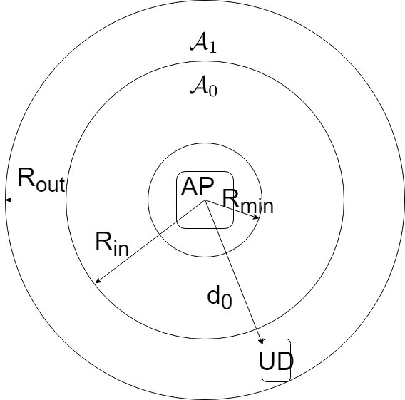
revsecII\zref@setcurrentrevcontentAs example of application of the N-P test we consider the scenario of Fig. 1, wherein area is a ring with smaller radius and larger radius and ROI is a ring concentric to , with larger radius and smaller radius . A single AP () is located at the ROI center and a UD is transmitting from distance . We consider two models: a) uncorrelated fading scenario, which includes LOS path-loss and spatially uncorrelated fading, and b) uncorrelated shadowing scenario, which includes LOS path loss and spatially uncorrelated shadowing. In both case, we consider the LOS model for path-loss. \zlabelsimpleScenAs example of application of the N-P test we consider the scenario of Fig. 1, wherein area is a ring with smaller radius and larger radius and ROI is a ring concentric to , with larger radius and smaller radius . A single AP () is located at the ROI center and a UD is transmitting from distance . We consider two models: a) uncorrelated fading scenario, which includes LOS path-loss and spatially uncorrelated fading, and b) uncorrelated shadowing scenario, which includes LOS path loss and spatially uncorrelated shadowing. In both case, we consider the LOS model for path-loss. \zref@setcurrentrevsecII\zref@setcurrentrevcontentIn order to compute \zlabelsimpleScen2In order to compute 222Note that for a single AP vector becomes the scalar . \zref@setcurrentrevsecII\zref@setcurrentrevcontent, we first observe that the PDF of incurring in attenuation for a user located inside the ROI is (by the total probability law) \zlabelsimpleScen2_0, we first observe that the PDF of incurring in attenuation for a user located inside the ROI is (by the total probability law)
| (8) |
revsecII\zref@setcurrentrevcontentwhere is the PDF of the UD transmitting from distance inside the ROI. Assuming that UD position is uniformly distributed in , and letting and , we have for , and otherwise. \zlabelsimpleScen2_1where is the PDF of the UD transmitting from distance inside the ROI. Assuming that UD position is uniformly distributed in , and letting and , we have for , and otherwise. \zref@setcurrentrevsecII\zref@setcurrentrevcontentA similar expression holds for . \zlabelsimpleScen2_2A similar expression holds for . Closed-form expressions of the LLR in the two scenarios are derived in Appendix A.
revsecII\zref@setcurrentrevcontentWe can see that obtaining LLRs needs the computation of various integrals evein in this simple case. Therefore, in general (e.g., with either multiple APs or correlated shadowing/fading), the LLR can not be computed in closed-form, thus making N-P test problematic. \zlabelllrCompWe can see that obtaining LLRs needs the computation of various integrals evein in this simple case. Therefore, in general (e.g., with either multiple APs or correlated shadowing/fading), the LLR can not be computed in closed-form, thus making N-P test problematic.
II-D Estimated Distance Approach
revsecII\zref@setcurrentrevcontentWe will compare our IRLV solutions with the estimated distance approach (EDA) of [6]. In EDA, first the estimate of the UD-AP distance is obtained by inverting the path-loss formula, and then the UD position is estimated as \zlabelliterature_1We will compare our IRLV solutions with the EDA of [6]. In EDA, first the estimate of the UD-AP distance is obtained by inverting the path-loss formula, and then the UD position is estimated as
| (9) |
revsecII\zref@setcurrentrevcontentLet be the set of points of the border of , and let the estimated distance of the UD from the border , where the sign is negative if , and positive otherwise. Lastly, is compared with a suitable threshold , chosen in order to achieve a desired FA probability, resulitng in , , otherwise. \zlabelliterature_2Let be the set of points of the border of , and let the estimated distance of the UD from the border , where the sign is negative if , and positive otherwise. Lastly, is compared with a suitable threshold , chosen in order to achieve a desired FA probability, resulitng in , , otherwise. \zref@setcurrentrevsecII\zref@setcurrentrevcontentNote that this approach requires the knowledge of the path-loss model (including knowledge of LOS and non-LOS state), which is quite unrealistic. Moreover, the estimator (9) is not optimal, since the position error is usually not a Gaussian variable. \zlabelliterature_3Note that this approach requires the knowledge of the path-loss model (including knowledge of LOS and non-LOS state), which is quite unrealistic. Moreover, the estimator (9) is not optimal, since the position error is usually not a Gaussian variable.
III IRLV by Machine Learning Approaches
The application of the N-P theorem requires the knowledge of the conditional PDFs at the APs, which can be hard to obtain also because a-priori assumptions on them may be quite unrealistic. \zref@setcurrentrevsecIII\zref@setcurrentrevcontentTherefore, we propose to use a supervised ML approach \zlabelsupervisedTherefore, we propose to use a supervised ML approach operating in two phases:
-
•
Learning phase: the APs collect attenuation vectors from a trusted UD moving both inside and outside the ROI, while the UD reports its position to the APs. In this way, the APs can learn the behaviour of the attenuation in both regions and .
-
•
Exploitation phase: the APs verify the location of an un-trusted UD by the attenuation’s estimate, using the data acquired in the learning phase.
The learning phase works as follows: for each training attenuation vector , , collected during the learning phase, there is an associated label , , where if the trusted UD is in region , and if the trusted UD is in region . Vector collects the labels of all the attenuation vectors in the training phase. Given these data, the AP learns the function that provides the decision for each attenuation vector . Then, in the exploitation phase, the IRLV algorithm computes for a new attenuation vector and takes the decision between the two hypotheses. Note that our solution does not explicitly evaluate the PDF and the LLR, but rather directly implements the test function.
revsecIII\zref@setcurrentrevcontentWe stress the fact that the channel model of Section II-A provides a realistic communication scenario, while the analysis that follows is general, as no specific channel statistics are assumed. \zlabelframework2We stress the fact that the channel model of Section II-A provides a realistic communication scenario, while the analysis that follows is general, as no specific channel statistics are assumed.
In the rest of this Section, we briefly review the MLP NN and the SVM, describe the learning process and show that in asymptotic conditions (infinite training attenuation vectors, sufficiently complex models, and proper learning phase convergence) both MLP and SVM functions approximate the LLR function (6).
III-A Neural Networks
A NN is a function mapping a set of real values into real values. A NN processes the input in stages, named layers, where the output of one layer is the input of the next layer. Layer with (column vector) input is denoted as input layer, layer with (column vector) output is denoted as output layer, while intermediate layers are denoted as hidden layers. We denote as the number of hidden layers. Each layer , has outputs obtained by processing the inputs with functions named neurons. The output of the neuron of layer is , where the mapping between the input and the outputs is given by the activation function . The argument of the activation function is a weighted linear combination, with (row vector) weights , of the outputs of the previous layer plus a bias . We focus here on feedforward NNs, i.e., without loops between neurons’ input and output, an architecture also known as MLP. For an in-depth description of NNs refer for example to [23, Chapter 6].\zref@setcurrentrevsecIII\zref@setcurrentrevcontentActivation functions are typically chosen before training, while vectors are adapted according to the NN learning algorithm in order to minimize the loss function. \zlabelhyper1Activation functions are typically chosen before training, while vectors are adapted according to the NN learning algorithm in order to minimize the loss function.
In our setting, the input of the NN is the attenuation vector , , and the output layer has a single neuron () providing as output the scalar . Let be the output of the NN corresponding to the attenuation vector input . A threshold is used on the NN output to obtain the test function
| (10) |
revsecIII\zref@setcurrentrevcontentParameter shall be chosen in order to obtain the required FA probability. The value of which guarantees a certain FA probability can obtained by simulation, whereas it can not be obtained by inverting the FA probability function. This is due to the fact that the ML framework is applied when there is no knowledge of the distribution of the variables and hence we can not compute a closed-form expression of the FA probability \zlabellambdaNNParameter shall be chosen in order to obtain the required FA probability. The value of which guarantees a certain FA probability can obtained by simulation, whereas it can not be obtained by inverting the FA probability function. This is due to the fact that the ML framework is applied when there is no knowledge of the distribution of the variables and hence we can not compute a closed-form expression of the FA probability .333Notice that usually, for zero-one loss function, literature assumes . However, this choice provides the control of neither FA nor MD probabilities.
revsecIII\zref@setcurrentrevcontentBased on the loss function to be optimized during training NNs can solve different problems, and we consider here two widely used loss functions: MSE and CE. \zlabelceNeededBased on the loss function to be optimized during training NNs can solve different problems, and we consider here two widely used loss functions: MSE and CE.
III-B NN MSE Design
revsecIII\zref@setcurrentrevcontentAs optimal hypothesis testing is implemented via the N-P framework, which exploits the knowledge of the LLR function, we aim at learning this function from data. This problem is referred to as curve fitting and it can be solved by training a NN via the MSE loss function [24]. \zlabelceNeeded2As optimal hypothesis testing is implemented via the N-P framework, which exploits the knowledge of the LLR function, we aim at learning this function from data. This problem is referred to as curve fitting and it can be solved by training a NN via the MSE loss function [24]. According to the MSE design criterion, the MLP parameters are updated in the training phase in order to minimize the MSE [24]
| (11) |
This is achieved by using the stochastic gradient descent algorithm [25, Section 3.1.3].
In order to prove the connection of NN classifier with MSE design with the N-P test, we first recall the following theorem [26]
Theorem 1 (see [26]).
Let be the Bayes optimal discriminant function
| (12) |
Then the MLP trained by backpropagation via (11) minimizes the error .
revsecIII\zref@setcurrentrevcontentHence, Theorem 1 proves that in the presence of i) perfect training, ii) an infinite number of neurons, and iii) convergence of the learning algorithm to the minimum error, the function implemented by MLP is the Bayes optimal discriminant function. Now we have the following corollary. \zlabelteoruck2Hence, Theorem 1 proves that in the presence of i) perfect training, ii) an infinite number of neurons, and iii) convergence of the learning algorithm to the minimum error, the function implemented by MLP is the Bayes optimal discriminant function. Now we have the following corollary.
Corollary 1.
Consider an MLP with training converged to the global minimum of the MSE, by using an infinite number of training points (). Then the test function (10) provides the N-P test, thus it is the most powerful test.
Proof.
From the Bayes rule we have
| (13) |
Now, function (10) imposes a threshold on and reorganizing terms we obtain when
| (14) |
which is equivalent to the N-P criterion, except for a fixed scaling of the threshold. ∎
revsecIII\zref@setcurrentrevcontentNote that this result is quite general and can be applied to NNs with any number of layers and neurons, and any parameter adaptation approach, as long as the target design function is the MSE. Thus, Corollary 1 is suited also to describe the asymptotic behaviour of elaborate solutions, such as deep learning NNs. \zlabelrev11bNote that this result is quite general and can be applied to NNs with any number of layers and neurons, and any parameter adaptation approach, as long as the target design function is the MSE. Thus, Corollary 1 is suited also to describe the asymptotic behaviour of elaborate solutions, such as deep learning NNs.
III-C NN CE Design
revsecIII\zref@setcurrentrevcontentBinary classification aims at assigning labels or to input vectors. In this case, the usual choice for the loss function is the CE between the NN output and the true labels of the input vector \zlabelceNeeded3Binary classification aims at assigning labels or to input vectors. In this case, the usual choice for the loss function is the CE between the NN output and the true labels of the input vector [25, Chapter 5.2]
| (15) |
We now prove the connection of CE design criterion with the N-P theorem.
Theorem 2.
Consider an MLP with training converged to the global minimum of the CE, by using an infinite number of training points (). Then the test function (10) provides the N-P test, thus it is the most powerful test.
Proof.
The probability of being in hypothesis given the attenuation vector satisfies When training is performed with the CE loss function, the output of the MLP is the minimum MSE approximation of the probability of being in hypothesis , given the attenuation vector [25, Section 5.2], i.e., where the approximation is in the MSE sense. An alternative proof of this is given by [27].
Now, by using the threshold function (10), we have which can be rewritten as (with
| (16) |
| (17) |
By using (10) on the output of the NN designed with the CE criterion, under the convergence hypothesis, (17) coincides (except for a different threshold value) with (12), the function implemented by the NN trained with the MSE criterion. Therefore, from Corollary 1 we conclude that also the CE design criterion provides a test function equivalent the N-P test function. ∎
III-D Support Vector Machines
A SVM [25, Chapter 7] is a supervised learning model that can be used for classification and regression. We focus here on binary classification to solve the IRLV problem. The SVM implements the function
| (18) |
where is a feature-space transformation function, is the weight column vector and is a bias parameter. The test function is again provided by (10), where now is given by (18). Note that in the conventional SVM formulation, we have , while here is chosen according to the desired FA probability. \zref@setcurrentrevsecIII\zref@setcurrentrevcontentWhile the feature-space transformation function is chosen before training [25, Chapter 7], vector must be properly learned from the data to obtain the desired hypothesis testing. \zlabelhyper2While the feature-space transformation function is chosen before training [25, Chapter 7], vector must be properly learned from the data to obtain the desired hypothesis testing.
We consider the LS-SVM approach [28] for the optimization of the SVM parameters. Learning for LS-SVM is performed by solving the following optimization problem
| (19a) | |||
| (19b) |
revsecIII\zref@setcurrentrevcontentwhere is not optimized by the learning algorithm, but must be tuned on training data using a separate procedure, e.g., see [29]. \zlabelhyper3where is not optimized by the learning algorithm, but must be tuned on training data using a separate procedure, e.g., see [29]. In conventional SVM, variables , , are constrained to be non-negative and appear in the objective function without squaring. Inequalities in the constraints translate into a quadratic programming problem, while equalities constraints in LS-SVM yield a linear system of equations in the optimization values. In [30], it is shown that SVM and LS-SVM are equivalent under mild conditions. From constraints (19) and the fact that we have
| (20) |
that is the squared error between the soft output of the LS-SVM and the correct training label .
We now prove the equivalence between the LS-SVM and N-P classifiers. Let us first consider the following lemma that establishes the convergence of the learning phase of SVM, as .
Lemma 1.
For a large number of training samples taken with a given static probability distribution from a finite alphabet , i.e., for , the vector of the LS-SVM converges in probability to a vector of finite norm .
Proof.
See the Appendix B. ∎
We can now prove the following theorem establishing the optimality of the SVM solution, as it provides the most powerful N-P test for a given FA probability.
Theorem 3.
revsecIII\zref@setcurrentrevcontentConsider a LS-SVM with training converged to the global minimum of , and using an infinite number of training points drawn from the finite alphabet . \zlabelrevGOConsider a LS-SVM with training converged to the global minimum of , and using an infinite number of training points drawn from the finite alphabet . Then the test function (10) with (18) provides the N-P test, thus it is the most powerful test.
Proof.
From (19a) consider
| (21) |
where is the expected value computed with respect to the training points , as goes to infinity. The first equality in (21) comes from Lemma 1: since converges to a finite norm, we can write The last equality comes from the strong law of large numbers. In the limit, the optimization problem (19) is equivalent to
| (22) |
where we dropped constraints (19) by using (20). The optimization problem is the same as of NN design and from [26], with the pair minimizing (22) and parametrizing (18), we have Lastly, we exploit Corollary 1 to conclude the N-P-optimality of LS-SVM. ∎
In summary, we have proven that both NN (with CE and MSE design) and SVM (with LS design) converge to the N-P test function as the training set size goes to infinity, thus establishing their asymptotic optimality and their relation to the theory of most powerful hypothesis testing.
III-E Computational Costs of ML Approaches
revsecIII\zref@setcurrentrevcontentIn this section, we briefly review the computational cost for i) training each machine and ii) making a prediction on a new data point. Let be the number of epochs (how many times each training point is used) of a NN. \zlabelcomp1In this section, we briefly review the computational cost for i) training each machine and ii) making a prediction on a new data point. Let be the number of epochs (how many times each training point is used) of a NN.
revsecIII\zref@setcurrentrevcontentFor a basic fully connected feed-forward NN, the backpropagation training algorithm is when the number of neurons of each hidden layer is proportional to the input size, while the prediction of a new unseen data point is . For a more detailed analysis, which takes into account also the cost of the choice of the activation function, see [31]. \zlabelcomp2For a basic fully connected feed-forward NN, the backpropagation training algorithm is when the number of neurons of each hidden layer is proportional to the input size, while the prediction of a new unseen data point is . For a more detailed analysis, which takes into account also the cost of the choice of the activation function, see [31].
revsecIII\zref@setcurrentrevcontentFor a LS-SVM, the estimate of the vector at training time is found by solving a linear set of equations (instead of the traditional quadratic programming of SVM). In general, the computational cost is ; however, there are more efficient solutions that reduce this complexity to (see [32]). At test time, the prediction is linear in the number of features and the number of training points, i.e., . \zlabelcomp3For a LS-SVM, the estimate of the vector at training time is found by solving a linear set of equations (instead of the traditional quadratic programming of SVM). In general, the computational cost is ; however, there are more efficient solutions that reduce this complexity to (see [32]). At test time, the prediction is linear in the number of features and the number of training points, i.e., .
IV IRLV By One-class Classification
revsecIV\zref@setcurrentrevcontentIn practice, collecting training points from region may be difficult, since this region may be large and not necessarily well defined (being simply the complement of ). \zlabelrevOCIn practice, collecting training points from region may be difficult, since this region may be large and not necessarily well defined (being simply the complement of ). \zref@setcurrentrevsecIV\zref@setcurrentrevcontentTherefore, during the training phase, we collect attenuation vectors only from inside and use them to train a ML classifier to distinguish between vectors belonging to and in the testing phase. \zlabeloneClassTherefore, during the training phase, we collect attenuation vectors only from inside and use them to train a ML classifier to distinguish between vectors belonging to and in the testing phase. This problem can also be denoted as one-class classification, since we have only samples taken from one of the two classes of the problem to train the models.
In the following, we address the problem of one-class classification implemented via both NN and SVM. Two approaches are considered: the AE, using a NN, and the one-class least-square SVM (OCLSSVM).
Before proceeding, we consider the optimal approach when only the channel statistics from within are known a-priori. In this case the LLR (6) can not be used as discriminant function, as is not known. We can instead resort to the GLRT [22], which, although in general sub-optimal, is a meaningful generalization of the N-P test, providing the test function
| (23) |
IV-A Auto Encoder NN
revsecIV\zref@setcurrentrevcontentWe consider the AE [33], i.e., a NN trained to copy the input to the output. It comprises an encoder NN (with layers), which transforms the -dimensional input data into the -dimensional code, with , and a decoder NN (with layers), which reconstructs the original high-dimensional data from the low-dimensional code. For an in-depth description of the AE architecture, please refer to [23, Chapter 14]. When implementing AEs, it is convenient to use linear activation functions at the last hidden layer of the decoder [23, Chapter 14]. \zlabeldeep aeWe consider the AE [33], i.e., a NN trained to copy the input to the output. It comprises an encoder NN (with layers), which transforms the -dimensional input data into the -dimensional code, with , and a decoder NN (with layers), which reconstructs the original high-dimensional data from the low-dimensional code. For an in-depth description of the AE architecture, please refer to [23, Chapter 14]. When implementing AEs, it is convenient to use linear activation functions at the last hidden layer of the decoder [23, Chapter 14]. Note that the AE output is a vector of the same size of the AE input, and one-class classification is obtained by computing the reconstruction error between the input and the output of the AE and comparing its absolute value with a chosen threshold.
For our IRLV problem, we train the AE with attenuation vectors taken only when the trusted UD is in ROI . Then, by letting be the output vector of the AE for the attenuation input , the MSE is
| (24) |
Finally, the IRLV test function is
| (25) |
where again must be chosen to achieve a desired FA probability.
revsecIV\zref@setcurrentrevcontentAs the AE attempts to copy the input to its output, in the testing phase only vectors with features similar to those of the training set will be reconstructed with smaller MSE, whereas input vectors with different features will be mapped to different vectors at the output, with large MSE. Since training is based on vectors collected from area and we want to verify users located inside , by thresholding the MSE, we can obtain the desired classifier. \zlabelmseThresholdingAs the AE attempts to copy the input to its output, in the testing phase only vectors with features similar to those of the training set will be reconstructed with smaller MSE, whereas input vectors with different features will be mapped to different vectors at the output, with large MSE. Since training is based on vectors collected from area and we want to verify users located inside , by thresholding the MSE, we can obtain the desired classifier.
About the test power of the AE, we observe that it can be seen as the quantizer (or compression process) of an -dimensional signal into an -dimensional signal. In order to minimize the MSE of the reconstruction error, inputs with higher probability will have smaller quantization regions. Moreover, as the number of quantization points goes to infinity (since the quantization indices are in the continuous -dimensional space) all points in the same quantization region will have approximately the same probability. However, the quantization error for points within each region will be different for each point; in particular, equal to zero for the quantization point and greater than zero at the edges of the quantization region. Thus, we can conclude that the AE can not provide as output the PDF of the input, even with infinite training and an infinite number of neurons, as required by the GLRT decision rule (23). On the other hand, input points with a smaller PDF belong to larger quantization regions for which the reconstruction error is on average larger; therefore, the output provided by the AE is on average monotonically decreasing with the PDF of the input point.
IV-B One-Class LS-SVM
We can also resort to SVM to perform the one-class classification in IRLV: we focus in particular on the OCLSSVM, first introduced in [34] as an extension of the one-class SVM [35]. The only difference with respect to the SVM introduced in Section III is that the training optimization problem is now
| (26a) | |||
| (26b) |
Note that in the one-class case, the bias parameter appears also in the objective function.
We observe that also for OCLSSVM we can not establish a correspondence with GLRT. Nevertheless, by resorting to the Chernoff bound, we can conclude that by minimizing the MSE we also minimize the upper bound of the FA probability; therefore, the optimization process goes in the right direction although being not optimal.
V Numerical Results
In this section, we present the performance of the proposed IRLV methods, obtained from both experimental data and the channel models of Section II. We consider a unitary transmitting power for each user and a carrier frequency of GHz, and m for all the APs, unless differently specified. When spatial correlation of shadowing is assumed, we consider a decorrelation distance of m according to the model of Section II. The training points for the classification tasks are taken uniformly over the area ().
For the LS-SVM we use a Gaussian kernel function [25, Chapter 6]. \zref@setcurrentrevsecV\zref@setcurrentrevcontentFor the NN approach we use fully connected networks. For the two-class classification problem, the activation function of the input layer is the identity function, while the activation function of neurons in the hidden and output layers is the sigmoid [23, Section 6.2.2.2]. \zlabelactivationFor the NN approach we use fully connected networks. For the two-class classification problem, the activation function of the input layer is the identity function, while the activation function of neurons in the hidden and output layers is the sigmoid [23, Section 6.2.2.2]. \zref@setcurrentrevsecV\zref@setcurrentrevcontentNNs have been trained only for CE loss function, as we have shown in Corollary 1 and Theorem 2 that with both MSE and CE loss functions we achieve the same performance of the N-P test. \zlabelnumResSimplScen3NNs have been trained only for CE loss function, as we have shown in Corollary 1 and Theorem 2 that with both MSE and CE loss functions we achieve the same performance of the N-P test.
V-A Two-class IRLV With Single AP
We start with a IRLV system using a single AP.
Uncorrelated fading/shadowing
revsecV\zref@setcurrentrevcontentFirstly, we consider the environment of Section II-C describing a small area. The channel model includes spatially uncorrelated fading or shadowing, with m, m, and m. Moreover, LOS is assumed for path-loss. For uncorrelated fading, we consider two path-loss coefficients, namely and ; the closed-form expression of the LLRs for the N-P test are given by (28) and (30). With spatially uncorrelated shadowing, we set , and three values of shadowing standard deviation, namely dB, dB, and 6 dB; the closed-form expression of the LLRs for the N-P test is given by (32). For the ML approaches, we consider training points and a NN with hidden layers, each layer with neurons in layer . \zlabelnumResSimplScenFirstly, we consider the environment of Section II-C describing a small area. The channel model includes spatially uncorrelated fading or shadowing, with m, m, and m. Moreover, LOS is assumed for path-loss. For uncorrelated fading, we consider two path-loss coefficients, namely and ; the closed-form expression of the LLRs for the N-P test are given by (28) and (30). With spatially uncorrelated shadowing, we set , and three values of shadowing standard deviation, namely dB, dB, and 6 dB; the closed-form expression of the LLRs for the N-P test is given by (32). For the ML approaches, we consider training points and a NN with hidden layers, each layer with neurons in layer .
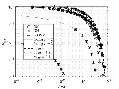
revsecV\zref@setcurrentrevcontentFig. 2 shows the FA probability versus the MD probability i.e., the detection error tradeoff (DET), obtained with the N-P test, the NN, and LS-SVM classifiers. We notice that all models achieve the same performance, confirming our theoretical results that both NN and LS-SVM with sufficient training data and number of hidden layers are optimal as N-P. \zlabelnumResSimplScen2Fig. 2 shows the FA probability versus the MD probability i.e., the detection error tradeoff (DET), obtained with the N-P test, the NN, and LS-SVM classifiers. We notice that all models achieve the same performance, confirming our theoretical results that both NN and LS-SVM with sufficient training data and number of hidden layers are optimal as N-P. \zref@setcurrentrevsecV\zref@setcurrentrevcontentWe observe that fading has more impact on the performance than shadowing, yielding higher FA and MD probabilities. Still, with fading, a higher path-loss coefficient provides better results, since the attenuation increases more with the distance, thus easing classification. For spatially uncorrelated shadowing, performance improves as decreases, since in this case path-loss alone already provides error-free decisions, thus the shadowing component is a disturbance in the decision process. \zlabelnumResSimplScen4We observe that fading has more impact on the performance than shadowing, yielding higher FA and MD probabilities. Still, with fading, a higher path-loss coefficient provides better results, since the attenuation increases more with the distance, thus easing classification. For spatially uncorrelated shadowing, performance improves as decreases, since in this case path-loss alone already provides error-free decisions, thus the shadowing component is a disturbance in the decision process.
Spatially correlated shadowing
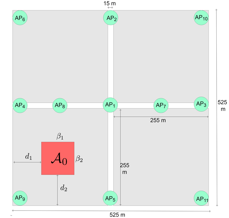
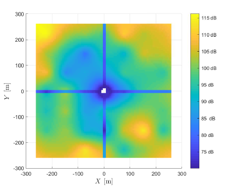
We now consider the spatially correlated shadowing ( dB) of Section II. The simulation environment is shown in Fig. 3, using only at the street intersection (while all other APs are not used) and a square ROI with m, m, and m. \zref@setcurrentrevsecV\zref@setcurrentrevcontentThe ROI is inside the south-west building, modelling for example a scenario wherein privileged network resources are accessible only to users inside an office. \zlabelbuildingThe ROI is inside the south-west building, modelling for example a scenario wherein privileged network resources are accessible only to users inside an office. Along the streets, LOS propagation conditions hold (with ), while non-LOS propagation conditions hold in the rest of the area. Fig. 4 shows a realization of the attenuation map (including both path-loss and shadowing), highlighting the different propagation conditions. Since no closed-form expression of the LLR is available in this scenario, we quantize the attenuations collected in the learning phase with a large alphabet and estimate the sampled PDF for the quantized attenuations. Lastly, we use the estimated PDF to compute the LLRs. We use training points in the area and a uniform quantizer for the attenuation (within the observed extreme values) with quantization values. Only points are used for training both the MLP and SVM.
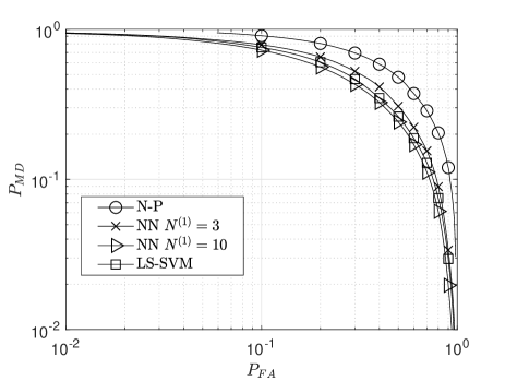
Fig. 5 shows the DET of N-P, NN, and LS-SVM, where for a given FA probability we report the MD probability averaged over the shadowing attenuation maps. We notice that both NN and LS-SVM outperform the N-P test. This means that, even for a very large number of samples available to estimate the PDF, we still have a performance degradation with respect to N-P with perfect knowledge of the statistics. On the other hand, with a small amount of training points the ML methods outperform N-P, without knowing the channel model. Therefore, in the following sections we drop the N-P method.
V-B Two-class IRLV With Multiple APs
We consider the environment of Fig. 3 with APs used for IRLV, namely with . The channel model includes LOS and non-LOS path-loss, spatially correlated shadowing ( dB), and fading, as described in Section II. We use a NN with hidden layers, each layer having neurons, .
No fading average
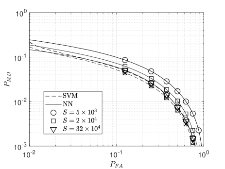
We first feed the learning machine with attenuation estimates obtained without fading average, i.e., . ROI position is m, m, and m. Fig. 6 shows the DET for NN and LS-SVM IRLV methods and different values of the training-set size . We observe that, for a given FA probability, the average MD probability decreases as the training-set size increases. Both ML models have similar performance with large training sets, confirming our result that they are both asymptotically optimal. However, SVM converges faster than NN (i.e., with a smaller ) to the optimal DET. Therefore, a careful design is needed for a practical implementation with finite training and limited computational capabilities. Note that we obtain a more accurate classification with multiple APs rather than using a single AP. Still, for security purposes, we would prefer even lower FA and MD probabilities; this can be achieved, for example, by increasing the number of APs or considering other channel features, e.g., its wideband impulse response.
revsecV\zref@setcurrentrevcontentWe have also considered a different ROI layout, with m, m and m. The ROI is still positioned in the south-west corner, but it includes both the crossroads and (see Fig. 3). Channel parameters are the same of Fig. 6. \zlabelrevnewareaWe have also considered a different ROI layout, with m, m and m. The ROI is still positioned in the south-west corner, but it includes both the crossroads and (see Fig. 3). Channel parameters are the same of Fig. 6. \zref@setcurrentrevsecV\zref@setcurrentrevcontentFig. 7 shows the resulting DET, still obtained by averaging the MD probabilities over the shadowing maps. Including the street inside the ROI, with its LOS path-loss, turns out to facilitate IRLV resulting in lower FA and MD probabilities. \zlabelnewarea2Fig. 7 shows the resulting DET, still obtained by averaging the MD probabilities over the shadowing maps. Including the street inside the ROI, with its LOS path-loss, turns out to facilitate IRLV resulting in lower FA and MD probabilities.
Effect of fading average
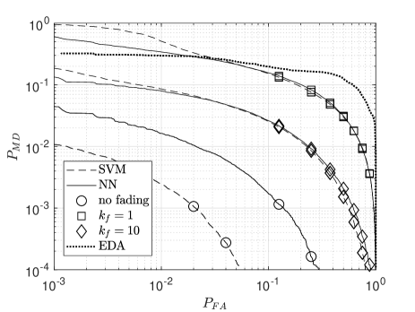
As discussed in Section II-A, for a given UD position, the attenuation changes over time due to fading. By averaging realizations of attenuation in the same position, the effect of fading on IRLV is mitigated. We consider the environment of Fig. 3 with APs used for IRLV, namely with , and the values of the channel parameters are those of Fig. 6. For explored locations by the UD we obtain training attenuation vectors. Fig. 8 shows the DET for and 10, with for SVM and for NN. \zref@setcurrentrevsecV\zref@setcurrentrevcontentWe also report the performance of EDA, assuming to know the path-loss relation between the attenuation and the distance. \zlabelrevLI2aWe also report the performance of EDA, assuming to know the path-loss relation between the attenuation and the distance. \zref@setcurrentrevsecV\zref@setcurrentrevcontentWe note that both MD and FA probabilities can be significantly reduced by averaging fading, thus approaching the performance on channels without fading. Indeed, an average of 10 fading realizations already reduces the average MD probability from to , for an FA probability of , while we achieve an average MD probability of without fading using a NN. We also notice that, in absence of fading, SVM significantly outperforms NN even if NN uses a larger . This suggests that, in this scenario, the NN has not yet converged to the optimum, wherein potentially very good performance can be achieved, due to limits in architecture, computational capabilities, and design algorithms. We should remember, in fact, that the number of parameters defining the SVM grows with the training size, while the number of parameters of the NN is set a-priori. \zlabelrev2fadWe note that both MD and FA probabilities can be significantly reduced by averaging fading, thus approaching the performance on channels without fading. Indeed, an average of 10 fading realizations already reduces the average MD probability from to , for an FA probability of , while we achieve an average MD probability of without fading using a NN. We also notice that, in absence of fading, SVM significantly outperforms NN even if NN uses a larger . This suggests that, in this scenario, the NN has not yet converged to the optimum, wherein potentially very good performance can be achieved, due to limits in architecture, computational capabilities, and design algorithms. We should remember, in fact, that the number of parameters defining the SVM grows with the training size, while the number of parameters of the NN is set a-priori. \zref@setcurrentrevsecV\zref@setcurrentrevcontentLastly, we observe that the proposed ML techniques (both with and without fading) outperform EDA, whose performance has been obtained on channels without fading. This is due to the fact that EDA is more severely affected by shadowing seen as disturbance in the derivation of the distance, while ML solutions may exploit it in making the decision, while still not relying on specific channel models. \zlabelrevLI2bLastly, we observe that the proposed ML techniques (both with and without fading) outperform EDA, whose performance has been obtained on channels without fading. This is due to the fact that EDA is more severely affected by shadowing seen as disturbance in the derivation of the distance, while ML solutions may exploit it in making the decision, while still not relying on specific channel models.
Results on experimental data
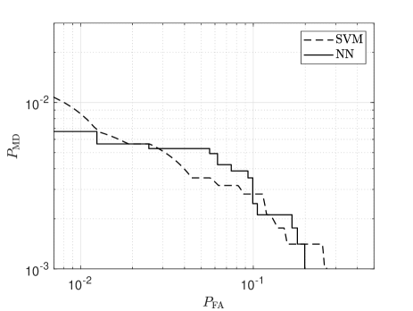
revsecV\zref@setcurrentrevcontentWe have tested the proposed IRLV solutions on real data collected by the MOMENTUM project [36] in a measurement campaign at Alexanderplatz in Berlin (Germany). Attenuations at the frequency of the global system for mobile communications (GSM) (that may refer to a cellular IoT scenario in our IRLV context) have been measured for several APs in an area of , on a measurement grid of m. We have considered 10 attenuation maps, corresponding to 10 AP positions (all in meters) , , , , , , , , , and . The ROI has been positioned in the lower-right corner, corresponding to, following the same notation of Fig 3, m, m, and m. In this case, we have a single realization of any channel effect (path-loss, shadowing, fading, …) per location, for a total of 8464 realizations, 5000 of which have been used for training and the rest for testing. For NN, we set and , . Fig. 9 shows the DET for both NN and LS-SVM. The performance is in line with the other figures obtained by simulation. Still, due to the small size of the available training set, DETs are not smooth. Moreover, we notice that SVM and NN achieve approximately the same performance. \zlabelBerlinWe have tested the proposed IRLV solutions on real data collected by the MOMENTUM project [36] in a measurement campaign at Alexanderplatz in Berlin (Germany). Attenuations at the frequency of the GSM (that may refer to a cellular IoT scenario in our IRLV context) have been measured for several APs in an area of , on a measurement grid of m. We have considered 10 attenuation maps, corresponding to 10 AP positions (all in meters) , , , , , , , , , and . The ROI has been positioned in the lower-right corner, corresponding to, following the same notation of Fig 3, m, m, and m. In this case, we have a single realization of any channel effect (path-loss, shadowing, fading, …) per location, for a total of 8464 realizations, 5000 of which have been used for training and the rest for testing. For NN, we set and , . Fig. 9 shows the DET for both NN and LS-SVM. The performance is in line with the other figures obtained by simulation. Still, due to the small size of the available training set, DETs are not smooth. Moreover, we notice that SVM and NN achieve approximately the same performance. \zref@setcurrentrevsecV\zref@setcurrentrevcontentNote also that, in order to use EDA, we should first know the path-loss to convert the attenuation estimates into distances, an information not immediately available from the experimental data. Therefore we could not compare ML with EDA in this case, further demonstrating the utility of ML model-less techniques for IRLV. \zlabelrevLINote also that, in order to use EDA, we should first know the path-loss to convert the attenuation estimates into distances, an information not immediately available from the experimental data. Therefore we could not compare ML with EDA in this case, further demonstrating the utility of ML model-less techniques for IRLV.
V-C One-Class IRLV With Multiple APs
We now focus on the one-class IRLV solutions, described in Section IV, where the training points come only from the ROI . \zref@setcurrentrevsecV\zref@setcurrentrevcontentThe AE has been designed according to [33], i.e., all neurons use the logistic sigmoid as activation function except for those in the central hidden layer, using linear activation functions. The AE has hidden layers with 7, 6, 3, 2, 3, 6, and 7 neurons, respectively. Weights are initialized randomly. \zlabeldesignAEThe AE has been designed according to [33], i.e., all neurons use the logistic sigmoid as activation function except for those in the central hidden layer, using linear activation functions. The AE has hidden layers with 7, 6, 3, 2, 3, 6, and 7 neurons, respectively. Weights are initialized randomly. The channel model is described in Section II, for the environment of Fig. 3 (with ), and the parameters of Section V-B, with m, m, and m.
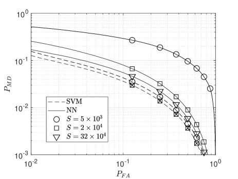
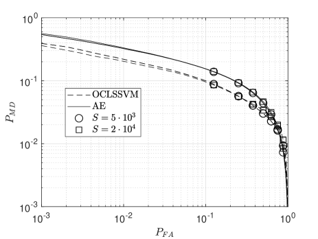
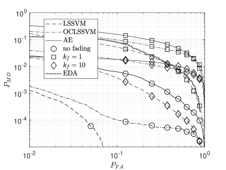
revsecV\zref@setcurrentrevcontentHere, we consider the effects of fading and the choice of the number of training points . Fig. 10 shows the DET for one-class IRLV systems for and two values of . We first notice that both AE and OCLSSVM converge for , and the SVM-based solution outperforms the NN-based solution, as already seen in the case of two-class classification. Fig. 11 shows the DET for and 10, while . We note that, for both ML techniques, averaging over fading significantly improves the performance. \zlabelfadingResHere, we consider the effects of fading and the choice of the number of training points . Fig. 10 shows the DET for one-class IRLV systems for and two values of . We first notice that both AE and OCLSSVM converge for , and the SVM-based solution outperforms the NN-based solution, as already seen in the case of two-class classification. Fig. 11 shows the DET for and 10, while . We note that, for both ML techniques, averaging over fading significantly improves the performance. \zref@setcurrentrevsecV\zref@setcurrentrevcontentWe also report the performance of EDA obtained without fading and assuming the knowledge of the path-loss relation between attenuation and distance. Again, we note that the proposed ML techniques significantly outperform EDA (in the absence of fading). \zlabelrevLI3We also report the performance of EDA obtained without fading and assuming the knowledge of the path-loss relation between attenuation and distance. Again, we note that the proposed ML techniques significantly outperform EDA (in the absence of fading). In the figure we also report the performance of two-class SVM for channels without fading: we can observe that, in the considered scenario, two-class IRLV outperforms the one-class IRLV: the former achieves a lower for the same . This result is expected since the two-class IRLV also exploits the (estimated) statistics of attenuation while under attacks.
VI Conclusions
In this paper, we have proposed innovative solutions for IRLV in wireless networks that exploit the features of the channels between the UD whose location must be verified by a trusted network of APs. By observing that in typical situations the channel statistics are not available for IRLV, we have proposed ML-based solutions, operating with both one- and two-class classification, i.e., with and without a-priori assumptions on attack statistics. For two-class classification we have proved that both NN and SVM solutions are the most powerful tests for a given sensitivity, i.e., they are equivalent to the N-P test. Instead, for one-class classification both AE and SVM solutions are not equivalent to the GLRT. We have also investigated how to collect the training points in order to be robust against the channel fading.
Appendix A LLRs derivation
A-1 Uncorrelated Fading scenario
revsecA\zref@setcurrentrevcontentAssuming spatially uncorrelated Rayleigh fading, without shadowing (i.e., , given a UD located at distance , the channel gain is exponentially distributed with mean (in dB) given by . Letting \zlabelsimpleScen3Assuming spatially uncorrelated Rayleigh fading, without shadowing (i.e., , given a UD located at distance , the channel gain is exponentially distributed with mean (in dB) given by . Letting
| (27) |
revsecA\zref@setcurrentrevcontentfrom the uniform UD distribution and (8) we have , whereas . \zlabelsimpleScen3_1from the uniform UD distribution and (8) we have , whereas . \zref@setcurrentrevsecA\zref@setcurrentrevcontentBy computing integrals for path-loss coefficient , the LLR is \zlabelsimpleScen3_2By computing integrals for path-loss coefficient , the LLR is
| (28) |
| (29) |
revsecA\zref@setcurrentrevcontentLet be the incomplete gamma function, then for we have instead \zlabelsimpleScen3_3Let be the incomplete gamma function, then for we have instead
| (30) |
A-2 Uncorrelated shadowing scenario
revsecA\zref@setcurrentrevcontentAssuming spatially uncorrelated shadowing, without fading we have , i.e., the received power from a given location is distributed in the logarithmic domain as a Gaussian random variable with mean value given by the path-loss (3) and standard deviation . Letting \zlabelsimpleScen4Assuming spatially uncorrelated shadowing, without fading we have , i.e., the received power from a given location is distributed in the logarithmic domain as a Gaussian random variable with mean value given by the path-loss (3) and standard deviation . Letting
| (31) |
revsecA\zref@setcurrentrevcontentfrom (8), the PDF of incurring an attenuation in hypothesis is , and . \zlabelsimpleScen4_1from (8), the PDF of incurring an attenuation in hypothesis is , and . \zref@setcurrentrevsecA\zref@setcurrentrevcontentBy solving the integral in (31) we obtain the LLR \zlabelsimpleScen4_2By solving the integral in (31) we obtain the LLR
| (32) |
revsecA\zref@setcurrentrevcontentwhere is the error function and \zlabelsimpleScen4_3where is the error function and
| (33) |
Appendix B Proof of Theorem 3
Given a finite attenuation vector alphabet of elements, with , we indicate with , with , the joint probability of input vector and corresponding output , .
By the Glivenko–Cantelli theorem we have that with probability 1 as there are training vectors with associated true label in any training sequence. All these training points will have the same error values , from (19b), that will appear times in the sum . Note that in the training ensemble there could be two equal instances , but with different labels . Therefore, for a given we can have two possible errors, depending on , and we denote them with and . This translates into only distinct constraints of type (19b). Asymptotically, for , problem (19) becomes
| (34) |
subject to and whose solution provides the convergence value (in probability) of vector . We write the Lagrangian
| (35) |
where are the Lagrangian multipliers. By setting to zero the derivatives with respect to we get the system of equations
| (36a) | |||
| (36b) | |||
| (36c) |
Note that (36) is a system with equations, linear in the unknowns and therefore has finite solution. In particular, we have
| (37) |
where we used the fact that the kernel function is symmetric with respect to its inputs. We conclude that has a finite norm since the right hand side of (37) is a finite sum.
References
- [1] Y. Zeng, J. Cao, J. Hong, S. Zhang, and L. Xie, “Secure localization and location verification in wireless sensor networks: a survey,” The Jour. of Supercomputing, vol. 64, no. 3, pp. 685–701, 11 2013.
- [2] G. Caparra, M. Centenaro, N. Laurenti, and S. Tomasin, “Optimization of anchor nodes’ usage for location verification systems,” in Proc. 2017 Int. Conf. on Localization and GNSS (ICL-GNSS), Nottingham, UK, 6 2017, pp. 1–6.
- [3] Y. Wei and Y. Guan, “Lightweight location verification algorithms for wireless sensor networks,” IEEE Trans. Parallel and Distributed Systems, vol. 24, no. 5, pp. 938–950, 5 2013.
- [4] L. C. et al., “Robustness, security and privacy in location-based services for future IoT: A survey,” IEEE Access, vol. 5, pp. 8956–8977, 4 2017.
- [5] E. A. Quaglia and S. Tomasin, “Geo-specific encryption through implicitly authenticated location for 5G wireless systems,” in Proc. 2016 IEEE 17th Int. Workshop on Signal Processing Advances in Wireless Commun. (SPAWC), Edinburgh, UK, 7 2016, pp. 1–6.
- [6] C. Li, F. Chen, Y. Zhan, and L. Wang, “Security verification of location estimate in wireless sensor networks,” in Proc. Int. Conf. on Wireless Commun. Networking and Mobile Computing (WiCOM), 9 2010, pp. 1–4.
- [7] E. Jorswieck, S. Tomasin, and A. Sezgin, “Broadcasting into the uncertainty: Authentication and confidentiality by physical-layer processing,” Proceedings of the IEEE, vol. 103, no. 10, pp. 1702–1724, 10 2015.
- [8] P. Baracca, N. Laurenti, and S. Tomasin, “Physical layer authentication over MIMO fading wiretap channels,” IEEE Trans. Wireless Commun., vol. 11, no. 7, pp. 2564–2573, 5 2012.
- [9] L. Xiao, Y. Li, G. Han, G. Liu, and W. Zhuang, “PHY-layer spoofing detection with reinforcement learning in wireless networks,” IEEE Trans. Vehic. Tech., vol. 65, no. 12, pp. 10 037–10 047, 12 2016.
- [10] S. Brands and D. Chaum, “Distance-bounding protocols,” in Proc. Workshop on the Theory and Application of Cryptographic Techniques. Lofthus, Norway: Springer, 7 1993, pp. 344–359.
- [11] D. Singelee and B. Preneel, “Location verification using secure distance bounding protocols,” in Proc. IEEE Int. Conf. on Mobile Adhoc and Sensor Systems, 2005., 12 2005, p. 7.
- [12] J.-H. Song, V. W. Wong, and V. C. Leung, “Secure location verification for vehicular ad-hoc networks,” in Proc. IEEE Global Telecommunications Conf., 12 2008, pp. 1–5.
- [13] N. Sastry, U. Shankar, and D. Wagner, “Secure verification of location claims,” in Proc. of the 2nd ACM workshop on Wireless security. San Diego (CA): ACM, 9 2003, pp. 1–10.
- [14] A. Vora and M. Nesterenko, “Secure location verification using radio broadcast,” IEEE Trans. Dependable and Secure Computing, vol. 3, no. 4, pp. 377–385, 10 2006.
- [15] A. Abdou, A. Matrawy, and P. C. van Oorschot, “CPV: Delay-based location verification for the Internet,” IEEE Trans. Dependable and Secure Computing, vol. 14, no. 2, pp. 130–144, 3 2017.
- [16] S. Yan, I. Nevat, G. W. Peters, and R. Malaney, “Location verification systems under spatially correlated shadowing,” IEEE Trans. Wireless Commun., vol. 15, no. 6, pp. 4132–4144, 2 2016.
- [17] T. M. Cover and J. A. Thomas, Elements of information theory. John Wiley & Sons, 2012.
- [18] L. Xiao, X. Wan, and Z. Han, “Phy-layer authentication with multiple landmarks with reduced overhead,” IEEE Trans. Wireless Commun., vol. 17, no. 3, pp. 1676–1687, 12 2018.
- [19] Y. Tian, B. Denby, I. Ahriz, P. Roussel, and G. Dreyfus, “Robust indoor localization and tracking using GSM fingerprints,” EURASIP Jour. on Wireless Commun. and Networking, vol. 2015, no. 1, p. 157, 6 2015.
- [20] “LTE; evolved universal terrestrial radio access (E-UTRA); radio frequency (RF) system scenarios,” 3GPP, TR 36.942 version 15.0.0 Release 15, Jul 2018.
- [21] A. Goldsmith, Wireless communications. Cambridge university press, Cambridge, 2005.
- [22] S. M. Kay, Fundamentals of Statistical Signal Processing: Estimation Theory. Upper Saddle River, NJ, USA: Prentice-Hall, Inc., 1993.
- [23] I. Goodfellow, Y. Bengio, and A. Courville, Deep learning. MIT press, Cambridge, 2016.
- [24] C. M. Bishop and C. Roach, “Fast curve fitting using neural networks,” Review of scientific instruments, vol. 63, no. 10, pp. 4450–4456, 6 1992.
- [25] C. M. Bishop, Pattern Recognition And Machine Learning. Springer, New York, 2006.
- [26] D. W. Ruck, S. K. Rogers, M. Kabrisky, M. E. Oxley, and B. W. Suter, “The multilayer perceptron as an approximation to a Bayes optimal discriminant function,” IEEE Trans. Neural Networks, vol. 1, no. 4, pp. 296–298, 12 1990.
- [27] A. Brighente, F. Formaggio, M. Centenaro, G. M. Di Nunzio, and S. Tomasin, “Location-verification and network planning via machine learning approaches,” arXiv e-prints, 11 2018.
- [28] J. A. Suykens and J. Vandewalle, “Least squares support vector machine classifiers,” Neural processing letters, vol. 9, no. 3, pp. 293–300, 6 1999.
- [29] X. Guo, J. Yang, C. Wu, C. Wang, and Y. Liang, “A novel LS-SVMs hyper-parameter selection based on particle swarm optimization,” Neurocomputing, vol. 71, no. 16-18, pp. 3211–3215, 10 2008.
- [30] J. Ye and T. Xiong, “SVM versus least squares SVM,” Artificial Intelligence and Statistics, pp. 644–651, 4 2007.
- [31] M. Bianchini and F. Scarselli, “On the complexity of neural network classifiers: A comparison between shallow and deep architectures,” IEEE Trans. Neural Networks and Learning Systems, vol. 25, no. 8, pp. 1553–1565, 8 2014.
- [32] T. van Gestel, J. A. Suykens, B. Baesens, S. Viaene, J. Vanthienen, G. Dedene, B. de Moor, and J. Vandewalle, “Benchmarking least squares support vector machine classifiers,” Machine Learning, vol. 54, no. 1, pp. 5–32, 1 2004.
- [33] G. E. Hinton and R. R. Salakhutdinov, “Reducing the dimensionality of data with neural networks,” Science, vol. 313, no. 5786, pp. 504–507, 7 2006.
- [34] Y.-S. Choi, “Least squares one-class support vector machine,” Pattern Recognition Letters, vol. 30, no. 13, pp. 1236–1240, 10 2009.
- [35] B. Schölkopf, J. C. Platt, J. Shawe-Taylor, A. J. Smola, and R. C. Williamson, “Estimating the support of a high-dimensional distribution,” Neural computation, vol. 13, no. 7, pp. 1443–1471, 7 2001.
- [36] H. G. et al., “Evaluation of reference and public scenarios,” IST-2000-28088 MOMENTUM, Tech. Rep. D5.3, 2003. [Online]. Available: http://www.zib.de/momentum/paper/momentum-d53.pdf