A First-Order Dynamical Transition in the displacement distribution of a Driven Run-and-Tumble Particle

Abstract

We study the probability distribution $P(X_{N}=X,N)$ of the total displacement $X_{N}$ of an $N$-step run and tumble particle on a line, in presence of a constant nonzero drive $E$. While the central limit theorem predicts a standard Gaussian form for $P(X,N)$ near its peak, we show that for large positive and negative $X$, the distribution exhibits anomalous large deviation forms. For large positive $X$, the associated rate function is nonanalytic at a critical value of the scaled distance from the peak where its first derivative is discontinuous. This signals a first-order dynamical phase transition from a homogeneous ‘fluid’ phase to a ‘condensed’ phase that is dominated by a single large run. A similar first-order transition occurs for negative large fluctuations as well. Numerical simulations are in excellent agreement with our analytical predictions.

1 Introduction

Recent years have seen immense theoretical and experimental interest in the study of ‘active’ systems, consisting of self-propelled individual particles [1, 2, 3, 4]. These active particles exhibit novel collective nonequilibrium pheomena, such as the motility induced phase separation (MIPS) [5, 6, 7, 8, 9, 10, 11], clustering effect [12], spontaneous segregation of mixtures of active and passive particles [13] and many other interesting effects. These collective effects arise from a combination of self-propulsion and interaction between the active particles. However, even in the absence of interactions between particles (noninteracting limit), the stochastic process associated with a single active particle is rather interesting due purely to the self-propulsion. This self-propulsion induces a memory or ‘persistence’ in the effective noise felt by the particle, leading often to interesting non-Markovian effects. At the level of individual particles, the simplest examples of such active particles are the so called active Brownian motion (ABM) or the ‘Run-and-Tumble’ particle (RTP) [for a recent pedagogical review, see [4]]. For a single ABM particle, both free as well as confined in a harmonic trap, there have been a number of recent theoretical and experimental studies in two dimensions on the position distribution [14, 15, 16, 17, 18, 19, 20], as well as on its first-passage properties [18]. In this paper, we will focus on the other well studied model of a single active particle, namely the RTP [5, 8, 10] in one dimension, but subjected to a constant external force $E>0$.

RTP process mimicks the typical motion of bacterias such as E. Coli [11]: a particle moves ballistically at a constant speed for random durations of time, called “runs”, until sudden changes of direction and speed take place, called “tumbles”. The tumbling occurs as a Poisson process with rate $\gamma$, i.e., the distribution of the duration of a single run between two successive tumblings is exponential with parameter $\gamma$. We will set $\gamma=1$ for the rest of the paper. We will focus here in one dimension. At the end of each tumbling, the particle chooses a new velocity drawn independently (from run to run) from a probability distribution funtion (PDF) $q(v)$, which is typically symmetric. In the standard RTP model known as the persistent random walk, $q(v)$ is chosen to be bimodal:

$$q(v)=\frac{1}{2}\,\left[\delta(v-v_{0})+\delta(v+v_{0})\right]\,.$$ (1)

In this model, the position $x(t)$ of the RTP evolves in time via

$$\frac{dx}{dt}=v_{0}\,\sigma(t)\,,$$ (2)

where $\sigma(t)=\pm 1$ is a dichotomous telegraphic noise that flips between the two states with a constant rate $\gamma=1$. This persistent random walk model has been studied extensively in the past and many properties are known, e.g. the propagator and the mean exit time from a finite interval, amongst other observables [21, 22]. In one dimension, there have been a number of recent theoretical studies on the first-passage properties of a free RTP [23, 24, 25, 26, 27, 28] and, very recently, for an RTP subjected to an external confining potential [29].

In this paper, we will study a variant of this standard RTP model in one dimension. In our model, while the duration of a run, say $\tau_{i}$ for the $i$-th run, is still exponentially distributed with rate $\gamma=1$, the actual motion during a ‘run’ is different. In our model there is an external force $E>0$ that drives the particle during a run. More precisely, at the begining of the $i$-th run, the particle again chooses a new velocity $v_{i}$ from a PDF $q(v)$ (which is not necessarily bimodal). Then starting with this initial velocity $v_{i}$, the particle moves via Newton’s second law during the run duration $0\leq t\leq\tau_{i}$

$$\frac{dx}{dt}=v(t);\,\quad\quad m\,\frac{dv}{dt}=E\,;\quad v(0)=v_{i}\,.$$ (3)

Thus we assume that there is no friction due to the environment (the particle’s motion is thus not overdamped as in standard Brownian motion). We will also set the mass $m=1$ for simplicity. Integrating Eq. (3) trivially, the displacement $x_{i}$ during the $i$-th run is given by

$$x_{i}=v_{i}\tau_{i}+\frac{E}{2}\,\tau_{i}^{2}\,$$ (4)

where both $\tau_{i}$ and $v_{i}$ are independent random variables, drawn respectively from $p(\tau)=e^{-\tau}\,\theta(\tau)$ and $q(v)$ which is arbitrary (albeit symmetric). For $E=0$ and $q(v)$ bimodal as in Eq. (1), our model reduces to the standard RTP. We will focus here on $E>0$ and Gaussian velocity distribution $q(v)=e^{-v^{2}/2}/\sqrt{2\pi}$, though our results on condensation (see later) will hold for a large class of velocity distributions $q(v)$, including the bimodel case discussed above. We consider $N$ successive runs. We work here in the ensemble where the total number $N$ of runs (or tumbles) is fixed, rather than the total time elapsed $t$. However, our results can be easily extended to constant time ensemble. In the presence of a constant force $E$, the total distance travelled by the particle after $N$ runs is

$$X_{N}=\sum_{i=1}^{N}x_{i}=\sum_{i=1}^{N}\left[v_{i}\tau_{i}+\frac{E}{2}\tau_{i}^{2}\right]$$ (5)

In this paper, we are interested in the PDF $P(X,N)={\rm Prob.}[X_{N}=X]$ of the total displacement for large $N$. Our main new result is that for $E>0$ and for a broad class of $q(v)$’s including the Gaussian and the bimodal distributions, the PDF $P(X,N)$, for large $N$, exhibits a non-analyticity as a function of $X$—signalling a condenation type first-order ‘phase transition’ in the system, as disussed below. We show that for the standard RTP, i.e, for $E=0$ and $q(v)$ bimodal as in Eq. (1), this interesting phase transition disappears. Our main results are summarized in the next section. Below we discuss some qualitative features of this PDF $P(X,N)$ for large $N$ and the physics behind the phase transition, before moving to a more quantitative detailed analysis in the later sections.

Due to the presence of a nonzero $E>0$, the PDF $P(X,N)$ is clearly asymmetric as a fuction of $X$ (see Fig. 1), and it has three regimes which are denoted as $I$, $II$ and $III$ in Fig. 1. In the central regime $II$, $P(X,N)$ describes the probability of typical fluctuations of $X$, while regimes $I$ and $III$ correspond to atypically large fluctuations of $X$ on the negative and the positive side respectively. A “kink”, which is shown schematically in Fig. 1 at $X=X_{c}$, separates the typical fluctuations regime ($II$) from positive large deviations (regime $III$). Another similar kink at $X=-X_{c}$ (see Fig. (1)) separates regimes $I$ and $II$ on the side of negative fluctuations. The main result of this paper is to demonstrate that this change in the nature of the fluctuations at $X=X_{c}$ corresponds to a dynamical first-order transition. A similar transition separates fluctuations in the center of the distribution from negative large deviations (at the second kink on the left at $X=-X_{c}$, although in this case the transition is “hidden” by an exponential prefactor $e^{-E|X|}$. In the central fluid regime $II$, the total distance $X$ is democratically distributed between $N$ individual runs of average sizes, while in regime $III$ (respectively in $I$) there is a large positive (negative) “condensate” (i.e., a single run that is large) that coexists with $(N-1)$ typical runs. By zooming in close to the kinks or the critical points, we show that $P(X,N)$ is described by an anomalous large deviation form near the kinks, with a local rate function that is continuous at the kink, but its first-derivative has a discontinuous jump (see the results of numerical simulations in Figs. 4)—thus signalling a first-order phase transition.

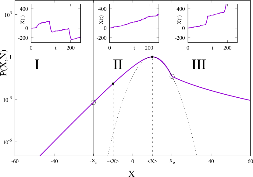
Figure 1: Main: Schematic representation of $P(X,N)$. Mean value is $\langle X\rangle=E\,N$. Vertical lines separates three regions, $I$, $II$ and $III$, corresponding respectively to $X<-X_{c}$, $-X_{c}\leq X<X_{c}$ and $X>X_{c}$. The two dynamical transitions are located at $X_{c}$ and $-X_{c}$. Region $II$ is the homogeneous phase. Regions $I$ and $III$ are the condensed phases. Dotted parabola is a guide to the eye. For $X\in[-\langle X\rangle,\langle X\rangle]$ (inside the dotted vertical lines), the PDF $P(X,N)$ is the result of a saddle-point approximation. Insets: typical trajectories for each of the three regions: homogeneous trajectories for $II$, dominated by one single run for $I$ and $III$.

Thus in our simple model, the PDF of the total displacement $P(X,N)$ exhibits a first-order phase transition, similar to the condensation transition that occurs in various lattice models of mass-transport [30, 31, 32, 33, 34, 35, 36, 37]. In these models, each site of a lattice (of $N$ sites) has a certain mass $m_{i}\geq 0$ and a fraction of the mass at each site gets transported to a neighbouring site with a rate that depends on the local mass—total mass $M$ is conserved by the dynamics. The Zero Range Process (ZRP) is a special case of these more general mass-transport models [30, 31, 32, 33]. The dynamics drives the system into a nonequilibrium steady state and there is a whole class of models for which the steady state has a product measure, i.e., the joint distribution of masses in the steady state becomes factorised [32]. Furthermore, under certain conditions, the system in the steady state undergoes a phase transition from a fluid phase for $M<M_{c}$, to a condensed phase $(M>M_{c})$ where one single site acquires a mass proportional to the total mass $M$ [32, 33]. This single site is the so called condensate.

The total distance $X$ travelled by an RTP in $N$ runs in our model is the counterpart to the total mass $M$ in mass-transport models on a lattice with $N$ sites. Hence, the condensate (a single site carrying a mass proportional to $N$) in the mass transport model corresponds to a single extensive run in the RTP model. One difference is that in mass-transport models, the mass $M$ is always positive, unlike in our case where $X$ can be both positive and negative. Consequently, we have both “positive” and “negative” condensates, while in the standard mass-transport models, there is only a “positive” condensate. This explains why we have a pair of critical points (see Figs. 1), as opposed to a single critical point in mass-transport models. Another difference lies in the observable of interest. In mass-transport models, the central object of interest is the mass distribution at a single lattice site and it shows different behaviors across the condensation transition. In our case we focus on a simpler object, the distribution $P(X,N)$ (playing the role of the partition function in mass-transport models with a factorised steady state), and we show how the signature of the condensation transition is already manifest in $P(X,N)$ itself. One of our main results is to show that near this critical point, $P(X,N)$ exhibits an anomalous large deviation form with an associated rate function that shows a discontinuity in its first derivative.

The rest of the paper is organized as follows. In Section 2, we define our model precisely and summarize the main results. Section 3 contains the most extensive analytical computation of the distribution $P(X,N)$ of the total displacement for $X>\langle X\rangle=EN$ (positive fluctuations). It also includes a discussion on the details of numerical simulations (Section 3.4). Section 4 contains analogus computation of $P(X,N)$ for $X<-\langle X\rangle=-EN$, i.e, for negative fluctuations. Section V contains a summary and conclusions. Finally, some details of the computations are presented in the Appendices.

2 The model and the summary of the main results

We consider a single RTP on a line, starting initially at $X=0$. Each trajectory is made of $N$ independent runs. The $i$-th run starts with initial velocity $v_{i}$ and lasts a random time $\tau_{i}$. The particle is also subjected to a constant force (field) $E>0$. The total displacement of the particle after $N$ runs, using Newton’s law for each run, is therefore given by

$$X_{N}=\sum_{i=1}^{N}x_{i}=\sum_{i=1}^{N}\left[v_{i}\tau_{i}+\frac{E}{2}\tau_{i}^{2}\right]\,$$ (6)

where $x_{i}$ denotes the displacement during the $i$-th run. The velocity $v_{i}$’s and the duration $\tau_{i}$’s for each run are i.i.d random variables drawn from the normalized PDF’s

$$q(v) =\frac{1}{\sqrt{2\pi}}\exp\left[-v^{2}/2\right]$$ (7)

$$p(\tau) =\Theta(\tau)\leavevmode\nobreak\ \exp(-\tau)$$ (8)

where $\Theta(t)$ is the Heaviside theta function: $\Theta(t)=1$ for $t\geq 0$ and $\Theta(t)=0$ for $t<0$. Even though we present detailed results only for the Gaussian velocity distribution $q(v)$ in Eq. (7), our main conclusions concerning the first-order phase transition is valid for a broad class of $q(v)$’s, including the bimodal distribution in Eq. (1). Our goal is to compute the probability distribution $P(X,N)={\rm Prob.}[X_{N}=X]$ of the total displacement $X_{N}=\sum_{i=1}^{N}x_{i}$. Thus, $X_{N}$ is clearly a sum of $N$ i.i.d. random variables. Each of the $x_{i}$’s has the normalized marginal PDF

$$\mathcal{P}(x)=\int_{-\infty}^{\infty}dv\leavevmode\nobreak\ \int_{0}^{\infty}d\tau\leavevmode\nobreak\ q(v)\,p(\tau)\,\delta(x-v\tau-E\tau^{2}/2)\,\,.$$ (9)

where $q(v)$ and $p(\tau)$ are given in Eqs. (7) and (8) respectively. The mean and the variance of the displacement during each run can be computed easily and one gets

$$\langle x\rangle =E$$ (10)

$$\sigma^{2} =\langle x^{2}\rangle-{\langle x\rangle}^{2}=2+5\,E^{2}$$ (11)

Computing explicitly $\mathcal{P}(x)$ from Eq. (9) is hard, however as we will see, what really matters for the large $N$ behavior of $P(X,N)$ is the asymptotic tail behavior of $\mathcal{P}(x)$. These tails can be explicitly obtained (see Appendix A). For large positive $x$ we get

$$\mathcal{P}(x\to\infty)\approx\frac{1}{E}e^{2/E^{2}}\,x^{-1/2}\,e^{-\sqrt{2x/E}}\ ,$$ (12)

and for large negative $x$

$$\mathcal{P}(x\to-\infty) =e^{-E\,|x|}\mathcal{P}(|x|)$$

$$\approx e^{-E\,|x|}\frac{e^{2/E^{2}}}{E}\,|x|^{-1/2}\,e^{-\sqrt{2|x|/E}}\ .$$ (13)

Thus the PDF $P(X_{N}=X,N)$ of the sum $X_{N}=\sum_{i=1}^{N}x_{i}$ reads

$$P(X,N)=\int_{-\infty}^{\infty}\left[\prod_{i=1}^{N}dx_{i}\leavevmode\nobreak\ \mathcal{P}(x_{i})\right]\leavevmode\nobreak\ \delta\left(X-\sum_{i=1}^{N}x_{i}\right).$$ (14)

where $\mathcal{P}(x)$ is given in Eq. (9).

Relation to mass transport models and a criterion for condensation transition. It is interesting to notice that $P(X,N)$ is formally similar to the partition function of lattice models of mass-transport with a factorised steady state [30, 31, 32, 33, 34, 35]. The latter reads as:

$$Z(M,N)=\int_{0}^{\infty}\left[\prod_{i=1}^{N}dm_{i}\leavevmode\nobreak\ f(m_{i})\right]\leavevmode\nobreak\ \delta\left(M-\sum_{i=1}^{N}m_{i}\right).$$ (15)

where $m_{i}\geq 0$ denotes the mass at site $i$, $f(m_{i})$ the corresponding steady state weight and $M$ being the total mass. Comparing Eqs. (14) and (15), and identifying the run distance $x_{i}$ with the mass $m_{i}$, $X$ with $M$, and $f(m_{i})$ with $\mathcal{P}(x_{i})$, we see that formally, our $P(X,N)$ is exactly the counterpart of the partition function $Z(M,N)$ in mass-transport models: the only difference is that, at variance with $m_{i}$’s which are non-negative variables, our $x_{i}$’s can be both positive and negative, which give rise to two condensed phases (respectively with a long positive and a long negative run).

Before discussing our strategy for the computation of $P(X,N)$ in Eq. (14) with $\mathcal{P}(x)$ given by (9), it is useful to recall, from the literature on the mass-transport models, which classes of $\mathcal{P}(x)$ may lead to the phenomenon of condensation. For the mass-transport models with positive mass $m$ distributed via the PDF $f(m)$ in Eq. (15), it is known [33] that a condensation occurs when the tail of $f(m)$ remains bounded in the interval $e^{-cm}<f(m)<1/m^{2}$, as $m\to\infty$, where $c>0$ is any positive constant. The ZRP typically corresponds to $f(m)\sim m^{-1-\mu}$ with $\mu>1$, and hence exhibits condensation [32, 33]. However, another class of $f(m)$’s that satisfy these bounds for large $m$ is the so called stretched exponential class: $f(m)\sim\exp\left[-a\,m^{\alpha}\right]$ for large $m$, with $\alpha>0$. Hence this class will also exhibit the condensation transition [34, 35]. In our RTP model with $p(\tau)=e^{-\tau}$ and $q(v)=e^{-v^{2}/2}/\sqrt{2\pi}$, we see that for large $x$, $\mathcal{P}(x)$ in Eq. (12) decays as a stretched exponential with the stretching exponent $\alpha=1/2$. Hence, we would expect a condensation transition for large positive $X$. A similar argument on the negative side shows that we will have a condensation transition for large negative $X$ as well. Hence, we expect that for any choice of $p(\tau)$ and $q(v)$ that leads via Eq. (9) to a marginal distribution $\mathcal{P}(x)$ which satisfies the bounds $e^{-c\,x}<\mathcal{P}(x)<1/x^{2}$ for large $x$, one will get a condensation. For example, for $E>0$, $p(\tau)=e^{-\tau}\theta(\tau)$ and with a bimodal velocity distribution $q(v)$ as in Eq. (1), it is easy to show (see Appendix A) that as $x\to\infty$,

$$\mathcal{P}(x)\sim\frac{1}{\sqrt{2\,E\,x}}\,e^{-\sqrt{2x/E}}\,,$$ (16)

which again satisfies the criterion for condensation. However, for the standard RTP model, i.e., if $E=0$, $p(\tau)=e^{-\tau}$ and $q(v)$ is bimodal as in Eq. (1), one finds (see Appendix A)

$$\mathcal{P}(x)=\frac{1}{2v_{0}}\,e^{-|x|/v_{0}}\,,$$ (17)

which does not satisfy the condensation criterion above. Hence, for the standard RTP, this condensation transition is absent. Thus, we see that while we present detailed calaculations only for the Gaussian velocity distribution, the phenomenon of condensation that we have found for the RTP model is robust: it occurs for a broad class of $p(\tau)$ and $q(v)$ that lead to a marginal $\mathcal{P}(x)$ satisfying the asymptotic bounds mentioned above. Incidentally, to the best of our knowledge, our model provides the first physical realization of the condensation belonging to this stretched exponential class.

Strategy for the large $N$ analysis of $P(X,N)$. Let us now briefly outline our strategy to compute analytically the PDF $P(X,N)$. By using the integral representation of the delta function: $\delta(X)=\int e^{s\,X}\,ds/(2\pi i)$, one can write $P(X,N)$ as

$$P(X,N) =\frac{1}{2\pi i}\int_{s_{0}-i\infty}^{s_{0}+i\infty}ds\leavevmode\nobreak\ e^{Nh(s)}$$

$$h(s) =sx+\log[\mathcal{L}(s)]$$ (18)

where $x=X/N$ and

$$\mathcal{L}(s) =\int_{-\infty}^{\infty}dx\,e^{-s\,x}\,\mathcal{P}(x)\,,$$

$$=\sqrt{\pi}\frac{e^{\frac{1}{2s(E-s)}}}{\sqrt{2s(E-s)}}\textrm{erfc}\left[\frac{1}{\sqrt{2s(E-s)}}\right].$$ (19)

where $\textrm{erfc}(z)=\frac{2}{\sqrt{\pi}}\,\int_{z}^{\infty}e^{-u^{2}}\,du$ is the complementary error function.

The integration contour in Eq. (18) is the Bromwich contour in the complex $s$ plane. There are two possible situations: (A) the equation $\partial h(s)/\partial s=0$ has a solution for real $s=s_{0}$ (see Fig. 3) and then the the integral in Eq. (18) can be computed for large $N$ using a saddle-point approximation; (B) there is no saddle point and one has to carry out the integration along the complex Bromwich contour. While the behaviour of $P(X,N)$ in case (A) has been already considered in [38], the accurate study of the PDF in case (B) is the original result of this paper: it is in this regime that the condensation takes place. Let us just mention that in regime (A), which corresponds to values $X\in[-\langle X\rangle,\langle X\rangle]$ with $\langle X\rangle=EN$ (see inside the homogeneous regime ($II$) in Fig. 1), the PDF $P(X,N)$ exhibits a large deviation form of the kind

$$P(X,N)\sim\exp\left\{-N\Phi\left(x=\frac{X}{N}\right)\right\},$$ (20)

where the rate function $\Phi(x)$ was computed numerically in [38]. It is easy to see, by virtue of central limit theorem [39], that in the vicinity of $X=\langle X\rangle=EN$ and similarly around $X=-\langle X\rangle=-EN$, the rate function simply reads

$$\Phi(x)=\begin{cases}\frac{(x-E)^{2}}{2\sigma^{2}},\quad\quad\quad\quad\,\,\,{\rm for}\,\,x\lesssim E\\ -Ex+\frac{(x+E)^{2}}{2\sigma^{2}},\quad{\rm for}\,\,x\gtrsim-E,\end{cases}$$ (21)

where $x=X/N$ and $E=\langle X\rangle/N$.

Consider now studying $P(X,N)$ in Eq. (18) as a function of increasing $X$. There is a saddle point $s_{0}$ on the real $s$ axis as long as $-\langle X\rangle<X<\langle X\rangle$. As $X\to\langle X\rangle$ from below, $s_{0}\to 0$. Similarly, as $X\to-\langle X\rangle$ from above, $s_{0}\to E$ (see Fig. 3). Our main interest in this paper is to study what happens when $X$ exceeds $\langle X\rangle$ on the positive side (respectively when $X$ goes below $-\langle X\rangle$ on the negative side), i.e., when there is no longer a saddle point on the real $s$ axis in the complex $s$ plane. A detailed study of the inverse Laplace transform in Eq. (18), when there is no saddle point, reveals a rich behavior of $P(X,N)$ for $X>\langle X\rangle$ (respectively for $X<-\langle X\rangle$).

Summary of the main results. Let us summarize our main results for $X>\langle X\rangle$ (detailed calculations are provided in Section III). Similar computations for $X<-\langle X\rangle$ are done in Section IV. It turns out that when $X$ exceeds $\langle X\rangle$ by $O(\sqrt{N})$, the behavior of $P(X,N)$ still remains Gaussian (as expected from the central limit theorem). Actually this Gaussian form continues to hold all the way up to $X-\langle X\rangle\sim N^{2/3}$. However, when $X-\langle X\rangle$ exceeds the critical value $X_{c}=z_{c}\,N^{2/3}$ (where $z_{c}$ is a constant of order $1$ that we compute explicitly), the Gaussian form ceases to hold. This is where the condensate starts to form. In this intermediate regime, where $X-\langle X\rangle=z\,N^{2/3}$ (where $z\sim O(1)$), $P(X,N)$ exhibits an anomalous large deviation form. Finally, in the extreme tail regime when $X-\langle X\rangle\sim O(N)$, where the system is dominated by one single large condensate, $P(X,N)$ has a stretched exponential form. These three behaviors are summarized as follows:

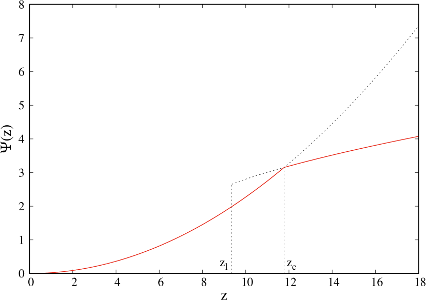
Figure 2: Continuous (red) line: rate function of Eq. (22), analytical prediction. $z_{c}\approx 11.78$ is the location of the first-order dynamical transition: $\Psi^{\prime}(z)$ is clearly discontinuous at $z_{c}$. Dotted lines indicates $\chi(z)$ for $z<z_{c}$ and $z^{2}/(2\sigma^{2})$ for $z>z_{c}$. $z_{l}$ is the lowest value of $z$ such that $\chi(z)$ can be computed via a saddle-point approximation.

$$P(X,N)\approx\begin{cases}e^{-(X-NE)^{2}/(2N\sigma^{2})}\quad{\rm for}\quad(X-EN)\sim N^{1/2}\\ e^{-N^{1/3}\Psi(z)}\quad\quad\quad\quad\leavevmode\nobreak\ {\rm for}\quad(X-EN)\sim N^{2/3}\\ e^{-\sqrt{2/E}\leavevmode\nobreak\ (X-EN)^{1/2}}\leavevmode\nobreak\ \leavevmode\nobreak\ {\rm for}\quad(X-EN)\sim N\\ \end{cases}$$

where $z=(X-EN)/N^{2/3}$. The rate function $\Psi(z)$ can be expressed as

$$\Psi(z)={\rm min}\left[\frac{z^{2}}{2\sigma^{2}},\chi(z)\right]$$ (22)

where the function $\chi(z)$ can be computed exactly (see Section III) in the regime $z\in[z_{l},\infty]$ with

$$z_{l}=\frac{3}{2}\left(\frac{\sigma^{4}}{E}\right)^{1/3}\,.$$ (23)

In this regime $z_{l}<z<\infty$, the function $\chi(z)$ has the asymptotic behaviors

$$\chi(z)=\begin{cases}\frac{3}{2}\left(\frac{\sigma}{E}\right)^{2/3}\qquad\qquad\qquad\qquad z\rightarrow z_{l}\\ \\ \sqrt{\frac{2}{E}}\sqrt{z}-\frac{\sigma^{2}}{4E}\frac{1}{z}+\mathcal{O}\left(\frac{1}{z^{5/2}}\right),\quad z\gg 1\end{cases}$$ (24)

The two competing functions $z^{2}/2\sigma^{2}$ and $\chi(z)$ in Eq. (22) are plotted in Fig. 2. Clearly, there exists a critical value $z=z_{c}$ where these two functions cross each other, such that one gets from Eq. (22)

$$\Psi(z)=\begin{cases}z<z_{c}\Longrightarrow z^{2}/(2\sigma^{2})\\ z>z_{c}\Longrightarrow\chi(z)\end{cases}.$$ (25)

where $z_{c}$ is given by the solution of the equation

$$\frac{z^{2}}{2\sigma^{2}}=\chi(z)$$ (26)

At $z=z_{c}$, the two functions match continuously, but the derivative $\Psi^{\prime}(z)$ is discontinuous at $z=z_{c}$ (see Fig. (2), signalling a first-order dynamical phase transition. The two functions cross each other at $z_{c}$, provided $z_{c}>z_{l}$. Indeed, by writing $z$ in units of $z_{l}$ and solving the matching condition in Eq. (26), we find that, independently of the value of $E$,

$${\color[rgb]{0,0,0}z_{c}=2^{1/3}\leavevmode\nobreak\ z_{l}},$$ (27)

which shows that $z_{c}>z_{l}$ for any choice of the field $E$. All the details on the computation of the function $\chi(z)$ and the determination of $z_{c}$ are given in Sec. 3 and in B.

Our analysis also clarifies that the mechanism of this dynamical transition is a typical one for a classic first-order phase transition: we show that the PDF $P(X,N)$, for $X-\langle X\rangle=z\,N^{2/3}$ where $z\sim O(1)$, can be written as a sum of two contributions,

$$P(X,N)=P_{\textrm{G}}(z,N)+P_{\textrm{A}}(z,N),$$ (28)

where $P_{\textrm{G}}(z,N)$ denotes Gaussian fluctuations, while $P_{\textrm{A}}(z,N)$ (where the subscript $A$ is for anomalous) denotes the rare fluctuations emerging from the formation of a condensate. These two terms compete with each other. In the vicinity of the transition point $z_{c}$ both contributions can be written in a large deviation form:

$$P_{\textrm{G}}(z,N) \sim e^{-N^{1/3}z^{2}/(2\sigma^{2})}$$

$$P_{\textrm{A}}(z,N) \sim e^{-N^{1/3}\chi(z)},$$ (29)

Since for $z<z_{c}$ one has $z^{2}/(2\sigma^{2})<\chi(z)$, see Fig. 2, then $\lim_{N\rightarrow\infty}P_{\textrm{A}}(z,N)/P_{\textrm{G}}(z,N)=0$: the Gaussian contribution dominates. On the contrary for $z>z_{c}$ one finds $z^{2}/(2\sigma^{2})>\chi(z)$ and the probability of the condensate takes over, i.e. $\lim_{N\rightarrow\infty}P_{\textrm{G}}(z,N)/P_{\textrm{A}}(z,N)=0$.

The accurate description of the first-order dynamical phase transition characterizing the tails of $P(X,N)$ is the main theoretical prediction of this paper. We have verified it via direct numerical simulations (see Fig. 4) and have found excellent agreement between numerics and theory.

3 First-order dynamical transition: calculation of the rate function

In this section, we compute the large $N$ behaviour of $P(X,N)$ for $X>\langle X\rangle$. The strategy consists in evaluating the leading contribution to the integral in Eq. (18) according to the scale of the deviation of $X$ from the average $\langle X\rangle$ that one is interested in. In particular we identify the three following regimes:

1. $X-\langle X\rangle\sim N^{1/2}$: the Gaussian regime.
   We discuss it in Sec. 3.1.

2. $X-\langle X\rangle\sim N$, the extreme large-deviation regime.
   This is discussed it in Sec. 3.2.

3. $X-\langle X\rangle\sim N^{2/3}$, the intermediate matching regime.
   We discuss it in Sec. 3.3.

In the Gaussian regime, for completeness, we also repeat how to compute $P(X,N)$ when $X<\langle X\rangle$ and $|X-\langle X\rangle|\sim N^{1/2}$, just to show that the result is consistent with fluctuations above the mean.

The three regimes listed above have one common feature: in order to compute $P(X,N)$, the Bromwich contour appearing in its integral representation in Eq. (18) must be deformed in order to pass around the branch cut on the negative semiaxis, see Fig. 3. In Fig. 3 are represented the analytical properties in the complex $s$ plane of $\mathcal{L}(s)$, the function defined in Eq. (18) and Eq. (19): it has two branch cuts on the real axis. The branch cut on the semiaxis $[E,\infty[$ is related to the behaviour of $P(X,N)$ for $X<-\langle X\rangle$, the branch cut on $]-\infty,0]$ to the behaviour for $X>\langle X\rangle$. In Fig. 3 are shown the examples of the two possible shapes of the Bromwich contour, depending on whether $X$ lies inside or outside the interval $[-\langle X\rangle,\langle X\rangle]$. For $X\in[-\langle X\rangle,\langle X\rangle]$ the Bromwich contour is a straight vertical line crossing the real axis at $s_{0}$, where $s_{0}$ is the saddle-point of the function $h(s)=sx+\log[\mathcal{L}(s)]$, with $x=X/N$. For $X\notin[-\langle X\rangle,\langle X\rangle]$ the contour must be deformed in order to pass around the branch cut.

In the following subsections we discuss the details of our calculations.

3.1 Gaussian Fluctuations

Let us start with the calculation of the probability of $\mathcal{O}(N^{1/2})$ fluctuations around $\langle X\rangle=EN$, considering separately the two cases $X<EN$ and $X>EN$. The result in the second case is that the non-analiticity at the branch cut is negligible, and the probability of fluctuations of order $|X-EN|\sim 1/\sqrt{N}$ is Gaussian also for $X>EN$. The general strategy of all the following calculations is to first fix the scale of the fluctuations $|X-EN|$ we are interested in, and then consider the corresponding orders in the expansion of $\mathcal{L}(s)$ around $s_{0}=0$.

We start by computing $P(X,N)$ for $X<EN$ and $|X-EN|\sim N^{1/2}$. The expansion of $\mathcal{L}(s)$ in Eq. (19) for small and positive $s$ reads:

$$\mathcal{L}(s)=1-Es+\frac{(1+3E^{2})}{2}s^{2}+\mathcal{O}(s^{3}),$$ (30)

from which one then gets

$$\log[\mathcal{L}(s)]=-Es+\frac{1}{2}\sigma^{2}s^{2}+\mathcal{O}(s^{3}),$$ (31)

where $\sigma^{2}=(2+5E^{2})$ is the second cumulant of the distribution $\mathcal{P}(x)$ defined in Eq. (9). Plugging the above expansions into integral of Eq. (18) one gets, for large $N$:

$$P(X,N)\approx\int_{s_{0}-i\infty}^{s_{0}+i\infty}\frac{ds}{2\pi i}e^{s(X-EN)+N\frac{\sigma^{2}}{2}s^{2}+\mathcal{O}(Ns^{3})}.$$ (32)

Since we are interested in evaluating the contribution to $P(X,N)$ at the scale $|X-EN|\sim N^{1/2}$, from $X$ and $s$ we change variables to $z$ and $\tilde{s}$:

$$X-EN =z\leavevmode\nobreak\ N^{1/2}$$

$$s =\tilde{s}/N^{1/2},$$ (33)

and then take the limit $N\rightarrow\infty$. All the irrelevant contributions vanish and one is left with a trivial Gaussian integral:

$$P(X,N)=\frac{1}{\sqrt{N}}\int_{-i\infty}^{i\infty}\frac{d\tilde{s}}{2\pi i}\leavevmode\nobreak\ e^{\tilde{s}z+\frac{\sigma^{2}}{2}\tilde{s}^{2}}=\frac{e^{-(X-EN)^{2}/(2\sigma^{2}N)}}{\sqrt{2\pi\sigma^{2}N}}.$$ (34)

The same result can be obtained in a straightforward manner with the saddle-point approximation.

More interesting is the calculation of $P(X,N)$ for $X>EN$. In this case the Bromwich contour needs to be deformed as shown in Fig. 3. Due to the presence of the branch cut $]-\infty,0]$, the expansion of $\mathcal{L}(s)$ in Eq. (19) is non-analytic at $s_{0}=0$ for $\textrm{Re}(s)<0$, in particular it yields different results for the positive and the negative imaginary semiplane:

$$\mathcal{L}(s+i0^{+}) =1-Es+(1+3E^{2})s^{2}+\ldots+\sqrt{\frac{2\pi}{sE}}e^{\frac{1}{2sE}+\frac{1}{2E^{2}}}$$

$$\mathcal{L}(s+i0^{-}) =1-Es+(1+3E^{2})s^{2}+\ldots$$

Accordingly, for the expansion of the logarithm one finds:

$$\log[\mathcal{L}(s+i0^{+})] =-Es+\frac{1}{2}\sigma^{2}s^{2}+\ldots+\sqrt{\frac{2\pi}{sE}}\leavevmode\nobreak\ e^{\frac{1}{2sE}+\frac{1}{2E^{2}}}$$

$$\log[\mathcal{L}(s+i0^{-})] =-Es+\frac{1}{2}\sigma^{2}s^{2}+\ldots$$

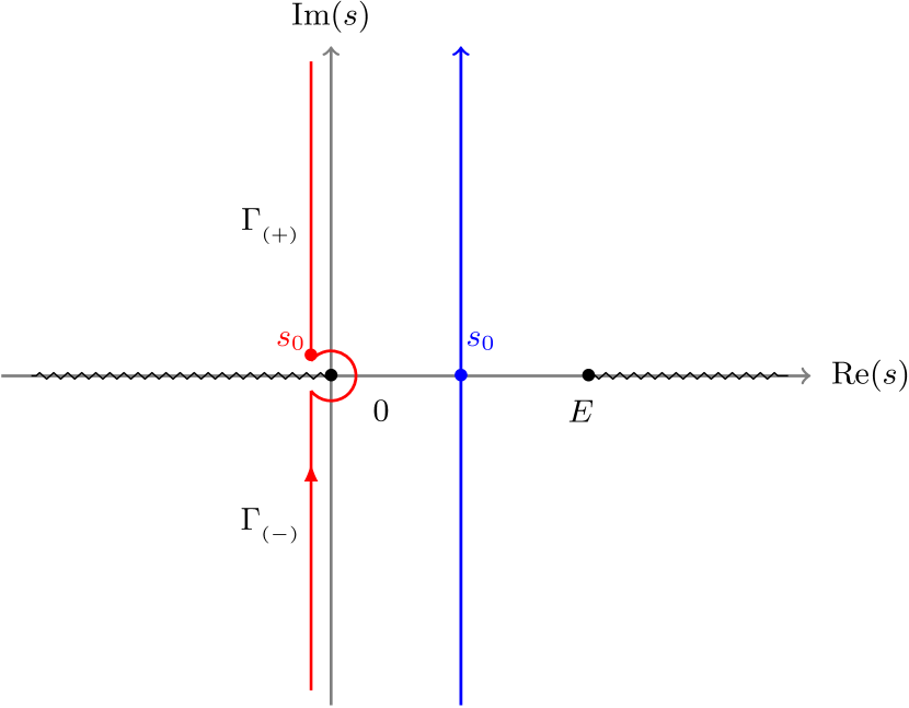
Figure 3: Analyticity structure of $\mathcal{L}(s)$, see Eq. (19), in the complex $s$ plane. Wiggled lines: the two branch cuts, respectively $]-\infty,0]$ and $[E,\infty[$. Straight (blue) line: Bromwich contour for the calculation of $P(X,N)$ when $-\langle X\rangle<X<\langle X\rangle$, with $s_{0}$ indicating the location of the saddle-point. Deformed (red) line: Bromwich contour to compute $P(X,N)$ when $X>\langle X\rangle$, $s_{0}$ indicates the new saddle point. $\Gamma_{(+)}$ and $\Gamma_{(-)}$ are labels for contour pieces in the positive and negative imaginary semiplanes.

Now, to compute $P(X,N)$ at the scale $X-EN\sim\sqrt{N}$ we consider separately the integration along the contour in the positive immaginary semiplane, denoted as $\Gamma_{{}_{(+)}}$ in Fig. 3, and along the contour in the negative semiplane, denoted as $\Gamma_{{}_{(-)}}$, so that

$$P(X,N)=\mathcal{I}_{(-)}+\mathcal{I}_{(-)},$$ (37)

where the symbols $\mathcal{I}_{(-)}$ and $\mathcal{I}_{(+)}$ denote respectively the contour integrations along $\Gamma_{{}_{(-)}}$ and $\Gamma_{{}_{(+)}}$. By plugging the expansions of Eq. (LABEL:eq:expansion_s_0) in the two integrals and changing of variables to $z=(X-EN)/N^{1/2}$ and $s=\tilde{s}/N^{1/2}$ one gets respectively:

$$\mathcal{I}_{(-)}=\frac{1}{\sqrt{N}}\int_{\Gamma_{{}_{(-)}}}\frac{d\tilde{s}}{2\pi i}e^{\tilde{s}z+\frac{\sigma^{2}}{2}\tilde{s}^{2}+\mathcal{O}(N^{-\frac{1}{2}})},$$

and

$$\mathcal{I}_{(+)}=\frac{1}{\sqrt{N}}\int_{\Gamma_{(+)}}\frac{d\tilde{s}}{2\pi i}e^{\tilde{s}z+\frac{\sigma^{2}}{2}\tilde{s}^{2}+\mathcal{O}(N^{-\frac{1}{2}})+N^{5/4}\sqrt{\frac{2\pi}{\tilde{s}E}}\leavevmode\nobreak\ e^{\frac{\sqrt{N}}{2\tilde{s}E}+\frac{1}{2E^{2}}}},$$

Since in the present case $\textrm{Re}(\tilde{s})<0$ the non-analytic contribution to the expansion of $\log[\mathcal{L}(s)]$ in Eq. (LABEL:eq:Gamma_minus_gauss) is exponentially small in $\sqrt{N}$ and can be neglected, so that to the leading order the integrands of $\mathcal{I}_{(-)}$ and of $\mathcal{I}_{(+)}$ are identical. By dropping also the terms $\mathcal{O}(N^{-\frac{1}{2}})$ in the argument of exponential one ends up with the formula:

$$P(X,N) =\frac{1}{\sqrt{N}}\int_{\Gamma_{{}_{(-)}}+\Gamma_{{}_{(+)}}}\frac{d\tilde{s}}{2\pi i}e^{\tilde{s}z+\frac{\sigma^{2}}{2}\tilde{s}^{2}}=\frac{1}{\sqrt{N}}\int_{-i\infty}^{i\infty}\frac{d\tilde{s}}{2\pi i}e^{\tilde{s}z+\frac{\sigma^{2}}{2}\tilde{s}^{2}}$$

$$=\frac{e^{-(X-EN)^{2}/(2\sigma^{2}N)}}{\sqrt{2\pi\sigma^{2}N}}.$$ (40)

The last equation completes the demonstration that at the scale $|X-EN|\sim N^{1/2}$ the distribution $P(X,N)$ is a Gaussian centered at $\langle X\rangle=EN$. This is, in fact, just a consequence of the validity of the central limit theorem.

3.2 Extreme Large deviation

We now focus on the extreme right tail of $P(X,N)$, where $X-NE\sim O(N)$. To compute the leading contributions to $P(X,N)$ on this scale, we change variables from from $X$ and $s$ to $z$ and $\tilde{s}$ as follows:

$$X-EN =z\leavevmode\nobreak\ N$$

$$s =\tilde{s}/N.$$ (41)

Also in this case, see for comparison Sec. 3.1, it is then convenient to split the integral expression of $P(X,N)$ in the positive and negative immaginary semiplane contributions, denoted respectively as $\mathcal{I}_{(+)}$ and $\mathcal{I}_{(-)}$. The function $\log[\mathcal{L}(s)]$ is not analytic at $s_{0}=0$ and for $\text{Re}(s)<0$ the expansions in the positive and negative semiplane are different and are those written in Eq. (LABEL:eq:expansion_s_0). Plugging in the definition of $\mathcal{I}_{(-)}$ and $\mathcal{I}_{(+)}$ the expressions of Eq. (LABEL:eq:expansion_s_0) and the change of variables of Eq. (41) one finds respectively

$$\mathcal{I}_{(-)}=\frac{1}{N}\int_{\Gamma_{{}_{(-)}}}\frac{d\tilde{s}}{2\pi i}e^{\tilde{s}z+\frac{\sigma^{2}}{2N}\tilde{s}^{2}+\mathcal{O}(N^{-2})}=\frac{1}{N}\int_{\Gamma_{{}_{(-)}}}\frac{d\tilde{s}}{2\pi i}e^{\tilde{s}z}\left[1+\frac{\sigma^{2}}{2N}\tilde{s}^{2}+\mathcal{O}(N^{-2})\right],$$ (42)

and

$$\mathcal{I}_{(+)}=\frac{1}{N}\int_{\Gamma_{{}_{(+)}}}\frac{d\tilde{s}}{2\pi i}e^{\tilde{s}z+\frac{\sigma^{2}}{2N}\tilde{s}^{2}+\mathcal{O}(N^{-2})+N^{3/2}\sqrt{\frac{2\pi}{\tilde{s}E}}e^{\frac{N}{2\tilde{s}E}+\frac{1}{2E^{2}}}}.$$ (43)

Note that all terms except $\tilde{s}z$ inside the exponential are small for large $N$ (including the term containing $e^{N/(2\tilde{s}E)}$, since the real part of $s$ is negative along the contour $\Gamma_{(+)}$). Hence, we can expand the exponential for large $N$. Keeping only leading order terms, we get

$$\mathcal{I}_{(+)}\approx\frac{1}{N}\int_{\Gamma_{{}_{(+)}}}\frac{d\tilde{s}}{2\pi i}e^{\tilde{s}z}\left[1+\frac{\sigma^{2}}{2N}\tilde{s}^{2}+\mathcal{O}(N^{-2})+N^{3/2}\sqrt{\frac{2\pi}{\tilde{s}E}}e^{\frac{N}{2\tilde{s}E}+\frac{1}{2E^{2}}}\right]$$

Summing the two contributions and grouping the analytic terms in the expansion one gets

$$\mathcal{I}_{(+)}+\mathcal{I}_{(-)} \approx\frac{1}{N}\int_{-i\infty}^{i\infty}\frac{ds}{2\pi i}e^{sz}\left[1+\frac{\sigma^{2}}{2N}s^{2}+\mathcal{O}(N^{-2})\right]+$$

$$+N^{1/2}\int_{\Gamma_{(+)}}\frac{ds}{2\pi i}e^{sz}\sqrt{\frac{2\pi}{sE}}\leavevmode\nobreak\ e^{\frac{N}{2sE}+\frac{1}{2E^{2}}}\,.$$ (45)

One can easily show that the integrals in the first line of Eq. (45) (coming from the analytic terms) all vanish. For example, the first term just gives a delta function $\delta(z)/N$ that vanishes for any $z>0$. The other analytic terms similarly can be evaluated using

$$\int_{-i\infty}^{i\infty}\frac{ds}{2\pi i}\leavevmode\nobreak\ e^{sz}\leavevmode\nobreak\ s^{n}=\delta^{(n)}(z)$$ (46)

and thus contribute Dirac delta’s derivatives of increasing order which all vanish for $z>0$.

Thus, the only nonvanishing contribution for large $N$ comes from the integral in the second line of of Eq. (45). To evaluate this integral, it is convenient to first rescale $s\to\sqrt{N}\,s$ and rewrite it as

$$\mathcal{I}_{(+)}+\mathcal{I}_{(-)}\approx N^{3/4}\sqrt{\frac{2\pi}{E}}\leavevmode\nobreak\ e^{\frac{1}{2E^{2}}}\int_{\Gamma_{(+)}}\frac{ds}{2\pi i}\leavevmode\nobreak\ \frac{1}{\sqrt{s}}\leavevmode\nobreak\ e^{\sqrt{N}(sz+\frac{1}{2sE})}\,.\\$$

To evaluate this integral, it is first convenient to rotate the contour $\Gamma_{(+)}$ anticlockwise by angle $\pi/2$. We are allowed to do this since the function is analytic in the left upper quadrant in the complex $s$ plane. So, the deformed (rotated) contour now runs along the real axis from $0$ to $-\infty$. This amounts to setting $s=-x$ with $x$ running from $0$ to $\infty$, and the integral in Eq. (3.2) reduces to an integral on the real positive axis $x\in[0,\infty]$

$$\mathcal{I}_{(+)}+\mathcal{I}_{(-)}\approx N^{3/4}\sqrt{\frac{1}{2\pi\,E}}\leavevmode\nobreak\ e^{\frac{1}{2E^{2}}}\int_{0}^{\infty}\frac{dx}{\sqrt{x}}\,e^{-\sqrt{N}\left(zx+\frac{1}{2xE}\right)}\,.$$ (47)

This integral can now be evaluated using the saddle point method. Defining,

$$u(x)=xz+\frac{1}{2xE}\,.$$ (48)

it is easy to check that $u(x)$ has a unique minimum at $x^{*}=1/\sqrt{2zE}$ (where $u^{\prime\prime}(x^{*})>0$). By plugging $x^{*}=-1/\sqrt{2zE}$ into the integral of Eq. (47) and evaluating carefully the integral (including the Gaussian fluctuations around the saddle point) [40, 41], we get, for large $N$ and with $z=(X-EN)/N$,

$$P(X,N)\approx N\leavevmode\nobreak\ e^{\frac{1}{2E^{2}}}\frac{\exp\left[-(2/E)^{1/2}\sqrt{(X-EN)}\right]}{\sqrt{2E(X-EN)}},$$ (49)

which is our final result for this section. Let us notice that the expression written in Eq. (49) is identical to $N$ times the asymptotic behaviour of the marginal probability distribution of the displacement in a single run, given in Eq. (12). This fact is perfectly consistent with the existence of a single positive condensate for $X-NE\sim O(N)$, that dominates the sum of $N$ i.i.d random variables each distributed via the marginal distribution; the combinatorial factor $N$ in front indicates that any one of the $N$ variables can be the condensate.

3.3 First-order transition: the intermediate matching regime

The main new result of this paper is the detailed study of the intermediate regime where Gaussian fluctuation and extreme large positive fluctuation both are of the same order: their competition is at the heart of the first-order nature of the dynamical transition that we find. This condition

$$\exp\left[-\frac{(X-EN)^{2}}{2\sigma^{2}N}\right]\sim\exp\left[-\sqrt{\frac{2}{E}}\sqrt{(X-EN)}\right],$$ (50)

simply sets the scale of the matching to be

$$X-EN\sim N^{2/3}.$$ (51)

As a consequence, in order to single out the leading contributions to $P(X,N)$ at this scale we must change variable from $X$ to $z$ in the integral of Eq. (18), with $z\sim O(1)$ such that:

$$X-EN=zN^{2/3}.$$ (52)

The trick is then to chose the proper rescaling of $s$ so that the analytic terms of the $\log[\mathcal{L}(s)]$ expansions (responsible for the Gaussian fluctuations), and the non-analytic ones (responsible for the anomalous fluctuations coming from the formation of the condensate), are of the same order. As is shown below, this is achieved by rescaling $s$ as

$$s=\tilde{s}/N^{1/3}.$$ (53)

Once again it is useful to evaluate separately the two contributions $\mathcal{I}_{(+)}$ and $\mathcal{I}_{(-)}$ after the change of variables. Taking into account the expansion of $\log[\mathcal{L}(s)]$ in Eq. (LABEL:eq:expansion_s_0) one gets respectively:

$$\mathcal{I}_{(-)} =\int_{\Gamma_{{}_{(-)}}}\leavevmode\nobreak\ \frac{ds}{2\pi i}\leavevmode\nobreak\ e^{sN^{2/3}z+N\frac{\sigma^{2}}{2}s^{2}+\mathcal{O}(Ns^{3})}$$

$$=\frac{1}{N^{1/3}}\int_{\Gamma_{{}_{(-)}}}\leavevmode\nobreak\ \frac{d\tilde{s}}{2\pi i}\leavevmode\nobreak\ e^{N^{1/3}\left(\tilde{s}z+\frac{\sigma^{2}}{2}\tilde{s}^{2}\right)+\mathcal{O}(1)},$$ (54)

and

$$\mathcal{I}_{(+)} =\int_{0}^{i\infty}\frac{ds}{2\pi i}\leavevmode\nobreak\ e^{s(X-NE)+N\frac{\sigma^{2}}{2}s^{2}+\mathcal{O}(Ns^{3})+{\color[rgb]{0,0,0}N}\sqrt{\frac{2\pi}{{\color[rgb]{0,0,0}s}E}}e^{\frac{1}{2{\color[rgb]{0,0,0}s}E}+\frac{1}{2E^{2}}}}$$

$$=\int_{0}^{i\infty}\frac{d\tilde{s}}{2\pi iN^{\frac{1}{3}}}\leavevmode\nobreak\ e^{N^{1/3}\tilde{s}z+N^{1/3}\frac{\sigma^{2}}{2}\tilde{s}^{2}+\mathcal{O}(1)+{\color[rgb]{0,0,0}N}\sqrt{\frac{2\pi N^{1/3}}{\tilde{s}E}}e^{\frac{N^{1/3}}{2\tilde{s}E}+\frac{1}{2E^{2}}}}$$

$$=\int_{0}^{i\infty}\frac{d\tilde{s}}{2\pi iN^{\frac{1}{3}}}\leavevmode\nobreak\ e^{N^{1/3}\tilde{s}z+N^{1/3}\frac{\sigma^{2}}{2}\tilde{s}^{2}}\left[1+{\color[rgb]{0,0,0}N}\sqrt{\frac{2\pi N^{1/3}}{\tilde{s}E}}e^{\frac{N^{1/3}}{2\tilde{s}E}+\frac{1}{2E^{2}}}\right].$$

By summing the expression of the two integrals in Eq. (54) and Eq. (LABEL:eq:Gamma_plus_matching) it is then easy to write $P(X,N)$, with $X-E\,N=z\,N^{2/3}$, explicitly as the sum of a Gaussian and an anomalous contribution:

$$P(X,N) =P_{\textrm{G}}(z,N)+P_{\textrm{A}}(z,N)$$

$$P_{\textrm{G}}(z,N) =\frac{1}{N^{1/3}}\int_{-i\infty}^{i\infty}\leavevmode\nobreak\ \frac{ds}{2\pi i}\leavevmode\nobreak\ e^{N^{1/3}\left(sz+\frac{\sigma^{2}}{2}s^{2}\right)}$$

$$P_{\textrm{A}}(z,N) =N^{5/6}\leavevmode\nobreak\ \frac{e^{1/(2E^{2})}}{i\sqrt{2\pi E}}\leavevmode\nobreak\ \int_{\Gamma_{{}_{(+)}}}ds\frac{1}{\sqrt{s}}\leavevmode\nobreak\ e^{N^{1/3}F_{z}(s)}$$

where the function $F_{z}(s)$ reads:

$$F_{z}(s)=sz+\frac{1}{2}\sigma^{2}s^{2}+\frac{1}{2sE}.$$ (57)

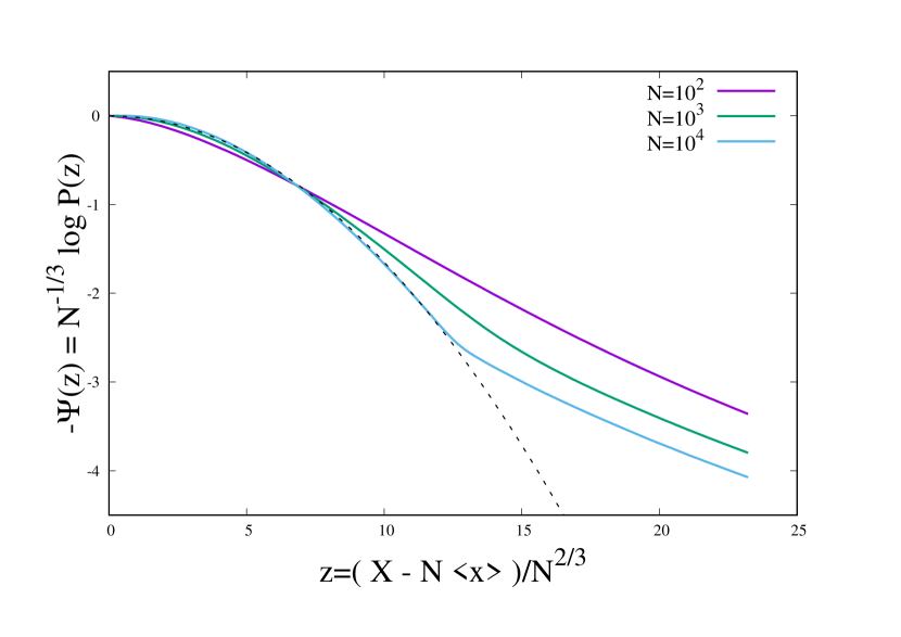
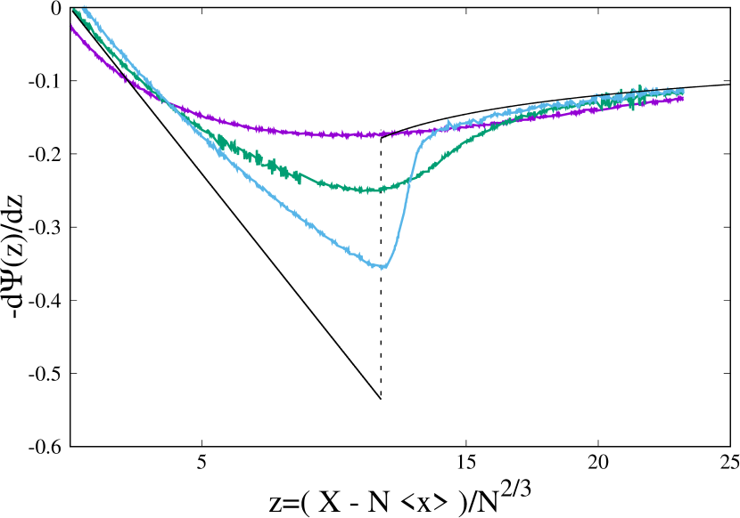
Figure 4: Top: numerical data for the rate function $\Psi(z)$. Different curves correspond to different number of runs $N$ in the trajectory: $N=10^{2},10^{3},10^{4}$. Acceleration is set to $E=2$. Dotted (black) line: guide to the eye, Gaussian (inverted) parabola. Bottom: numerical data for the rate function derivative $\Psi^{\prime}(z)$. Continuous black line is the analytical prediction in the limit $N\rightarrow\infty$, the coordinate of the transition point is $z_{c}\approx 11.78$ (for $E=2$).

The integral in the second line of Eq. (LABEL:eq:PX-matching) can be easily performed using the saddle point method, and gives a Gaussian contribution, justifying its name

$$P_{\textrm{G}}(z,N)\approx\frac{1}{\sqrt{2\pi\sigma^{2}N}}\,\exp\left[-N^{1/3}\,\frac{z^{2}}{2\sigma^{2}}\right]\,.$$ (58)

The integral in the second line of Eq. (LABEL:eq:PX-matching), giving rise to the anomalous part, can be also be computed with a saddle point approximation only when the saddle-point equation

$$\frac{\partial F_{z}(s)}{\partial s}=0$$ (59)

has a real root $s^{*}$. The real roots of Eq. (59) and their properties are studied in full detail in B. In the same appendix, we also discuss the domain of existence of the saddle point solution and give the explicit solution.

Skipping further details, we find that the saddle-point equation $F^{\prime}_{z}(s)=0$ has a real solution $s^{*}$ only for $z\in[z_{l},\infty]$, with $z_{l}=3\sigma^{4/3}/{2E^{1/3}}$ (see B): in this range the integral $P_{\textrm{A}}(z,N)$ can be explicitly evaluated. For $z<z_{l}$, computing the integral is hard as there is no saddle point on the real negative $s$ axis. However, as we will see, we do not need the information on $P_{\textrm{A}}(z,N)$ for $z=(X-EN)/N^{2/3}<z_{l}$. We will see that the transition occurs at $z=z_{c}>z_{l}$, so it is enough to compute $P_{\textrm{A}}(z,N)$ for $z>z_{l}$. Hence, for our purpose, evaluating $P_{\textrm{A}}(z,N)$ by saddle point is sufficient. Assuming the existence of a saddle point at $s=s^{*}$ and plugging the explicit expression of $s^{*}$ as a function of $z$ (see B) into Eq. (LABEL:eq:PX-matching) one gets:

$$P_{\textrm{A}}(z,N)\sim\leavevmode\nobreak\ e^{-N^{1/3}\chi(z)}.$$ (60)

The shape of the function $\chi(z)$ is shown in Fig. 2, where its behavior is compared with the parabola $z^{2}/(2\sigma^{2})$ of the Gaussian term. All the details on the derivation of $\chi(z)$ are in B. The asymptotics are:

$$\chi(z)=\begin{cases}\frac{3}{2}\left(\frac{\sigma}{E}\right)^{2/3}\qquad\qquad\qquad\qquad z\rightarrow z_{l}\\ \\ \sqrt{\frac{2}{E}}\sqrt{z}-\frac{\sigma^{2}}{4E}\frac{1}{z}+\mathcal{O}\left(\frac{1}{z^{5/2}}\right)\quad z\gg 1\end{cases}$$ (61)

Dropping the irrelevant prefactors aside, we then get

$$P(X,N)\approx\exp\left\{-N^{1/3}\frac{z^{2}}{2\sigma^{2}}\right\}+\exp\left\{-N^{1/3}\chi(z)\right\}.$$ (62)

The equation $z^{2}/(2\sigma^{2})=\chi(z)$ can be solved exactly with a simple argument (see B.3), yielding the following value of $z_{c}$ in units of $z_{l}$:

$${\color[rgb]{0,0,0}\frac{z_{c}}{z_{l}}=2^{1/3}}$$ (63)

In the numerical simulations we set the acceleration to $E=2$. By plugging this value in the expression of $z_{l}$ given in B we finally get:

$${\color[rgb]{0,0,0}z_{c}\approx 11.78},$$ (64)

the value indicated by the dotted vertical line in Fig. 4.

The mechanism of the first-order transition is now transparent. Recall that $X-EN=z\,N^{2/3}$. When $z<z_{c}$, the probability distribution $P(X,N)$ is dominated by the Gaussian contribution $P_{\textrm{G}}(z,N)$, since $z^{2}/(2\sigma^{2})<\chi(z)$. On the contrary for $z>z_{c}$ the distribution is dominated by the anomalous contribution $P_{\textrm{A}}(z,N)$, since $z^{2}/(2\sigma^{2})>\chi(z)$. The result can be summarized as follows:

$$z<z_{c} \Longrightarrow\frac{z^{2}}{2\sigma^{2}}<\chi(z)\Longrightarrow P(X,N)\approx e^{-N^{1/3}z^{2}/(2\sigma^{2})}$$

$$z>z_{c} \Longrightarrow\frac{z^{2}}{2\sigma^{2}}>\chi(z)\Longrightarrow P(X,N)\approx e^{-N^{1/3}\chi(z)}$$ (65)

Thus the mechanism behind the first order transition corresponds to a classic first-order phase transition scenario in standard thermodynamics: in the vicinity of the transition point there is a competition between two phases characterized by a different free-energy (here the value of the rate function) and the transition point itself is defined as the value of the control parameter (here the value of the displacement) where the free-energy difference between the two phases changes sign.

3.4 First-order transition from numerical simulations

The direct consequence of the description in Eq. (65) is that the rate function $\Psi(z)$, which is $\Psi(z)=z^{2}/(2\sigma^{2})$ for $z<z_{c}$ and $\Psi(z)=\chi(z)$ for $z>z_{c}$, has a discontinuity in its first-order derivative $\Psi^{\prime}(z)$ at $z_{c}$: this happens because the two functions $z^{2}/(2\sigma^{2})$ and $\chi(z)$ match continuously at $z_{c}$, but with a different slope.

We show in this section that the discontinuity of the rate function $\Psi(z)$ appears for large enough $N$ when one tries to sample numerically the tails of $P(X,N)$. We have studied the behaviour of $P(X,N)$ for $N=10^{2},10^{3},10^{4}$ runs in the trajectory. The behaviour of the rate function $\Psi(z)$ and of its derivative $\Psi^{\prime}(z)$ are shown in Fig. 4. While at $N=10^{2}$ the transition from the Gaussian to the large deviations regime is still a smooth crossover, the trend for increasing $N$ goes clearly towards a discontinuous jump of $\Psi^{\prime}(x)$. The location of the discontinuity revealed by the numerical simulations is in agreement with the analytic prediction $z_{c}\approx 11.78$ given for the value $E=2$.

Simulations are straightforward but one has to chose a clever strategy: just looking at the probability distribution of independent identically distributed random variables is not sufficient, since doing like that one can only probe the typical fluctuations regime, $|X-\langle X\rangle|\sim N^{1/2}$, but not the large deviations. In order to sample $P(X,N)$ in the whole regime of interest a set of many simulations is needed, each probing the behaviour of the PDF in a narrow interval $[X^{*},X^{*}+\Delta]$. We provide in what follows a detailed description of the numerical protocol.

In order to achieve an efficient sampling of $P(X,N)$ also in the matching and in the large deviations regime we follow here the strategy to compute the tails of random matrices eigenvalues distribution used in [45, 46]. The basic idea is to sample $P(X,N)$ in many small intervals $[X^{*},X^{*}+\Delta]$ varying $X^{*}$, in order to recover finally the whole distribution. The sampling of $P(X,N)$ in each interval $[X^{*},X^{*}+\Delta]$ corresponds to an independent Monte Carlo simulation. Since the total number of runs in the trajectory is fixed to $N$, for each value of $X^{*}$ we fix the initial condition chosing a set $(\tau_{1}^{\text{in}},\ldots,\tau_{N}^{\text{in}})$ of runs durations and a set $(v_{1}^{\text{in}},\ldots,v_{N}^{\text{in}})$ of initial velocities for each run such that:

$$\sum_{i=1}^{N}\left[v_{i}^{\text{in}}\tau_{i}^{\text{in}}+\frac{E}{2}(\tau_{i}^{\text{in}})^{2}\right]>X^{*}.$$ (66)

In the intial condition all the local variables are of order unit: $v_{i}^{\text{in}},\tau_{i}^{\text{in}}=\mathcal{O}(1)$. The stochastic dynamics to sample $P(X,N)$ in the vicinity of $X^{*}$ then goes on as any standard Metropolis algorithm: attempted updates are accepted or rejected with probability $p=\text{min}[1,p(\mathcal{C}^{\text{old}})/p(\mathcal{C}^{\text{new}})]$ where the stationary probability of a configuration $p(\mathcal{C})$ reads as:

$$p(\tau_{1},v_{1},\ldots,\tau_{N},v_{N})\approx\exp\left(-\sum_{i=1}^{N}\left[\tau_{i}+v_{i}^{2}/2\right]\right).$$ (67)

The only additional ingredient with respect to a standard Metropolis algorithm is that all attempts which brings $X_{N}$ below $X^{*}$ are rejected. The precise form of the probability distribution sampled for each value of $X^{*}$ in the Monte Carlo dynamics is therefore:

$$P(X,N|X>X^{*})=e^{-\sum_{i=1}^{N}[\tau_{i}+v_{i}^{2}/2])}\leavevmode\nobreak\ \Theta\left(\sum_{i=1}^{N}\left[v_{i}\tau_{i}+\frac{E}{2}\tau_{i}\right]-X^{*}\right),$$ (68)

where $\Theta(x)$ is the Heavyside step function.
We define as a Monte Carlo sweep the sequence of $N$ local attempts of the kind $(v_{i},\tau_{i})\leavevmode\nobreak\ \Rightarrow\leavevmode\nobreak\ (v_{i}^{\text{new}},\tau_{i}^{\text{new}})$ where

$$v_{i}^{\text{new}}=v_{i}+\delta v,$$

$$\tau_{i}^{\text{new}}=\tau_{i}+\delta\tau.$$ (69)

The shifts $\delta v$, $\delta\tau$ are random variables drawn from uniform distributions. Then, if and only if the constraint implemented by the Heavyside step function in Eq. (68) is satisfied, otherwise the attempt is rejected immediately, the new values $(v_{i}^{\text{new}},\tau_{i}^{\text{new}})$ are accepted with probability:

$$p_{\text{acc}}=\text{min}\left[1,e^{-\left[(v_{i}^{\text{new}})^{2}/2+\tau_{i}^{\text{new}}-(v_{i}^{2}/2+\tau_{i})\right]}\right].$$ (70)

In order to recover the full probability distribution $P(X,N)$ within the interval $X\in\mathcal{I}=[\langle X\rangle,\langle X\rangle+2z_{c}\langle X\rangle^{2/3}]$ we have divided $\mathcal{I}$ in a grid of $M=100$ elements. More precisely, we have run $M$ simulations for a set of equally-spaced values $X^{*}\in\mathcal{I}$. Each simulation allows one to sample $P(X,N|X>X^{*})$ only in a small interval on the right of $X^{*}$. The value $z_{c}$ is the critical one predicted by the theory. The choice of the interval $\mathcal{I}$ has been somehow arbitrary, we just took care that it was centered around the expected critical value $X_{c}$ for the condensation transition. We have taken a number of sweeps $N_{\text{sweeps}}\approx 10^{7}$, enough to forget the initial conditions.

The relation between the PDF $P(X,N|X>X^{*})$ sampled in the MC numerical simulations and the PDF we want to investigate, $P(X,N)$, is as follows:

$$P(X,N)=P(X,N|X>X^{*})\leavevmode\nobreak\ P(X>X^{*},N)$$ (71)

In particular, what we are interested in is the rate function $\Psi(z)$ defined as:

$$\Psi\left(z=\frac{X-\langle X\rangle}{N^{2/3}}\right)=-\frac{1}{N^{1/3}}\leavevmode\nobreak\ \log\left[P(X,N)\right].$$ (72)

The rate function $\Psi_{z^{*}}(z)$ that we measure in the vicinity of $X^{*}$ by sampling the probability distribution in Eq. (68) differs from the original one, due to Eq. (71), by an additive constant:

$$\Psi(z) =-\frac{1}{N^{1/3}}\log\left[P(X,N|X>X^{*})\right]-\frac{1}{N^{1/3}}\log\left[P(X>X^{*},N)\right]$$

$$=\Psi_{z^{*}}(z)+f(z^{*}),$$

where $f(z^{*})$ is a function that depends only on $z^{*}$. By taking the derivative with respect to $z$ (and taking into account that $dz=dX/N^{2/3}$) one gets rid of the additive constant and obtain the following expression:

$$\frac{d\Psi(z)}{dz}=\frac{d\Psi_{z^{*}}(z)}{dz}=-\frac{N^{1/3}}{P(X,N|X>X^{*})}\frac{dP(X,N|X>X^{*})}{dX}$$ (74)

Therefore what we have done has been to sample numerically $d\Psi_{z^{*}}(z)/dz$ in the vicinity of many values $z^{*}$ by means of the biased Monte Carlo dynamics. The function $\Psi(z)$ has been then obtained from the numerical integration of the first-order derivative. Both the rate function $\Psi(z)$ and its first derivative $\Psi^{\prime}(z)$ are shown in Fig. 4.

4 First-Order transition for negative fluctuations.

So far we focused only on the right tail of $P(X,N)$, but the probability distribution is not symmetric due to $E$, as is shown in the pictorial representation of Fig. 1. We need to comment also on the behaviour of the left tail of $P(X,N)$. In this section we demonstrate that even for negative fluctuations a first-order dynamical transition takes place, and that, following the same arguments of Sec. 3, it is located at $X_{c}^{(-)}=-X_{c}$, where $X_{c}=z_{c}N^{2/3}+NE$, with $z_{c}$ given in Eqs. (63) and (64). The location of the transition for negative fluctuations is symmetric to that for positive ones. The only difference with the case of positive fluctuations is that for $X<0$ the PDF has in front an exponential damping factor due to the field $E$. Here is the summary of the behavior of $P(X,N)$ in the three regimes, i.e. typical fluctuations, extreme large negative deviations and the intermediate matching regime, for $X<0$:

$$P(X,N)\approx\begin{cases}e^{-E|X|}\leavevmode\nobreak\ e^{-(X+NE)^{2}/(2N\sigma^{2})}\leavevmode\nobreak\ \leavevmode\nobreak\ {\rm for}\leavevmode\nobreak\ (X+EN)\sim N^{1/2}\\ e^{-E|X|}\leavevmode\nobreak\ e^{-N^{1/3}\Psi(z)}\quad\quad\quad\quad{\rm for}\leavevmode\nobreak\ (X+EN)\sim N^{2/3}\\ e^{-E|X|}\leavevmode\nobreak\ e^{-\sqrt{2/E}\leavevmode\nobreak\ |X+EN|^{1/2}}\leavevmode\nobreak\ \leavevmode\nobreak\ {\rm for}\leavevmode\nobreak\ (X+EN)\sim N\end{cases},$$

where $z=-(X+NE)/N^{2/3}$ and the rate function $\Psi(z)$ is the same as te one we have computed for positive fluctuations.

The calculations to obtain the behaviours in Eq. (LABEL:three-regimes-negative) are identical to those for $X>0$, which are described in full detail in Sec. (3) and in B. We are not going to repeat all of them here. We will sketch the derivation of the results in Eq. (LABEL:three-regimes-negative) only for the matching regime, which is the most interesting among the three. This discussion has also the purpose to highlight the (small) differences with the calculations in the case $X>0$, in particular to show where the prefactor $e^{-E|X|}$ comes from.

First, as can be easily noticed looking at Eq. (19), the function $\mathcal{L}(s)$ has the following symmetry

$$\mathcal{L}(s)=\mathcal{L}(E-s),$$ (76)

which is important for the following reason. To compute $P(X,N)$ for values of the total displacemente $X>EN$ we needed to wrap the Bromwich contour around the branch cut at $]-\infty,0]$ (see Fig. 3). This was done by taking the analytic continuation of $\log[\mathcal{L}(s)]$ in the complex plane in the neighbourhood of $s_{0}=0$. In the same manner, in order to compute $P(X,N)$ for $X<-NE$, we must wrap the Bromwich contour around the branch cut at $[E,\infty[$. To do this we need the analytic continuation of $\log[\mathcal{L}(s)]$ in the neighbourhood of $s_{0}=E$. Due to the symmetry in Eq. (76) the expansion of $\log[\mathcal{L}(s)]$ in the neighbourhood of $s_{0}=E$ is identical to the one in the neighbourhood of $s_{0}=0$, including the non-analyticities due to the branch cut. In particular we have that:

$$\log[\mathcal{L}(E-s+i0^{+})] =-E(E-s)+\frac{1}{2}\sigma^{2}(E-s)^{2}+\ldots+\sqrt{\frac{\pi}{2E(E-s)}}e^{\frac{1}{2s(E-s)}+\frac{1}{2E^{2}}}$$

$$\log[\mathcal{L}(E-s+i0^{-})] =-E(E-s)+\frac{1}{2}\sigma^{2}(E-s)^{2}+\ldots$$ (77)

As done in the case of positive fluctuations, also for $X<-NE$ is convenient to split the expression of the inverse Laplace transform of $P(X,N)$, see Eq. (18), in two contributions: the contour integral in the negative semiplane, $\mathcal{I}_{(-)}$, and the contour integral in the positive semiplane, $\mathcal{I}_{(+)}$. Let us consider first the integral $\mathcal{I}_{(-)}$:

$$\mathcal{I}_{(-)}=\int_{\Gamma_{(-)}}\frac{ds}{2\pi i}e^{sX+N\left[-E(E-s)+\frac{1}{2}\sigma^{2}(E-s)^{2}+\ldots\right]}.$$ (78)

In this case ($X<0$) is convenient to change variable from $s$ to $y=E-s$:

$$\mathcal{I}_{(-)} =\int_{-\Gamma_{(-)}}\frac{dy}{2\pi i}\leavevmode\nobreak\ e^{(E-y)X+N\left[-Ey+\frac{1}{2}\sigma^{2}y^{2}+\ldots\right]}$$

$$=e^{XE}\leavevmode\nobreak\ \int_{\Gamma_{(-)}}\frac{dy}{2\pi i}\leavevmode\nobreak\ e^{-y(X+EN)+N\frac{1}{2}\sigma^{2}y^{2}+\ldots}.$$ (79)

Then, in order to have a variable which is positive and is of order $\mathcal{O}(1)$ when $X+EN\sim N^{2/3}$ we introduce:

$$z=-\frac{X+EN}{N^{2/3}}.$$ (80)

By rescaling the integration variable $y=\tilde{y}/N^{\frac{1}{3}}$, appropriate for the matching intermediate regime, we can rewrite

$$\mathcal{I}_{(-)}=e^{EX}\leavevmode\nobreak\ \frac{1}{N^{1/3}}\int_{\Gamma_{(-)}}\frac{d\tilde{y}}{2\pi i}\leavevmode\nobreak\ e^{N^{1/3}\left[\tilde{y}z+\frac{1}{2}\sigma^{2}\tilde{y}^{2}\right]+\mathcal{O}(1)}.$$ (81)

The expression of $\mathcal{I}_{(-)}$ in Eq. (81), is, apart from the prefactor $e^{EX}$, identical to the analogous one evaluted for $X>0$, see Eq. (54). The only difference is that now the scaling variable $z$ is defined as $z=-(X+EN)/N^{2/3}$ rather than $z=(X-EN)/N^{2/3}$. In the same way for the integral in the positive complex semiplane we find:

$$\mathcal{I}_{(+)}=e^{EX}\frac{1}{N^{1/3}}\int_{\Gamma_{{}_{(+)}}}\frac{d\tilde{y}}{2\pi i}e^{N^{1/3}\left[\tilde{y}z+\frac{1}{2}\sigma^{2}\tilde{y}^{2}\right]+\ldots+N\sqrt{\frac{2\pi N^{1/3}}{E\tilde{y}}}e^{\frac{N^{1/3}}{2E\tilde{y}}+\frac{1}{2E^{2}}}}$$ (82)

Recalling that we are expanding for $\text{Re}(y)=\text{Re}(E-s)<0$ (see Fig.3), and hence $\tilde{y}<0$, we can further expand:

$$\mathcal{I}_{(+)} = e^{EX}\frac{1}{N^{1/3}}\int_{\Gamma_{{}_{(+)}}}\frac{d\tilde{y}}{2\pi i}e^{N^{1/3}\left[\tilde{y}z+\frac{1}{2}\sigma^{2}\tilde{y}^{2}\right]}\left[1+N\sqrt{\frac{2\pi N^{1/3}}{E\tilde{y}}}e^{\frac{N^{1/3}}{2E\tilde{y}}+\frac{1}{2E^{2}}}\right]$$

$$= e^{EX}\frac{1}{N^{1/3}}\int_{\Gamma_{{}_{(+)}}}\frac{d\tilde{y}}{2\pi i}e^{N^{1/3}\left[\tilde{y}z+\frac{1}{2}\sigma^{2}\tilde{y}^{2}\right]}+N^{5/6}\leavevmode\nobreak\ e^{EX}\leavevmode\nobreak\ \frac{e^{1/(2E^{2})}}{i\sqrt{2\pi E}}\int_{\Gamma_{{}_{(+)}}}\frac{d\tilde{y}}{\sqrt{\tilde{y}}}\leavevmode\nobreak\ e^{N^{1/3}F_{z}(\tilde{y})}$$

so that

$$\mathcal{I}_{(+)}+\mathcal{I}_{(-)} =e^{EX}\frac{1}{N^{1/3}}\int_{-i\infty}^{i\infty}\frac{d\tilde{y}}{2\pi i}e^{N^{1/3}\left[\tilde{y}z+\frac{1}{2}\sigma^{2}\tilde{y}^{2}\right]}+N^{5/6}\leavevmode\nobreak\ e^{EX}\leavevmode\nobreak\ \frac{e^{1/(2E^{2})}}{i\sqrt{2\pi E}}\int_{\Gamma_{{}_{(+)}}}\frac{d\tilde{y}}{\sqrt{\tilde{y}}}e^{N^{1/3}F_{z}(\tilde{y})}$$

$$F_{z}(\tilde{y}) =\tilde{y}z+\frac{1}{2}\sigma^{2}\tilde{y}^{2}+\frac{1}{2\tilde{y}E},$$ (84)

where the function $F_{z}(\tilde{y})$ is identical to that of Eq. (57), hence leading to the same conclusions. For negative fluctuations as well, it is then straightforward to see that in the intermediate matching regime we have two competing contributions, i.e. the Gaussian, $P_{\textrm{G}}(z,N)$, and anomalous one, $P_{\textrm{A}}(z,N)$:

$$P_{\textrm{G}}(z,N)=\frac{1}{N^{1/3}}\int_{-i\infty}^{i\infty}\frac{d\tilde{y}}{2\pi i}e^{N^{1/3}\left[\tilde{y}z+\frac{1}{2}\sigma^{2}\tilde{y}^{2}\right]}$$

$$P_{\textrm{A}}(z,N)=N^{5/6}\leavevmode\nobreak\ e^{EX}\leavevmode\nobreak\ \frac{e^{1/(2E^{2})}}{i\sqrt{2\pi E}}\int_{-i\infty}^{i\infty}\frac{d\tilde{y}}{\sqrt{\tilde{y}}}\leavevmode\nobreak\ e^{N^{1/3}F_{z}(\tilde{y})},$$ (85)

where $z=-(X+NE)/N^{2/3}$. The probability distribution for negative fluctuations in the matching regime reads therefore as:

$$P(X,N)=e^{EX}\left[P_{\textrm{G}}(z,N)+P_{\textrm{A}}(z,N)\right],$$ (86)

Apart from the prefactor $e^{EX}$ the expression of $P(X,N)$, for negative fluctuations in the matching regime, is the same as that for positive fluctuations: the condensation transition at $z_{c}$ is driven by the same mechanism, the competition between the Gaussian fluctuations of $P_{\textrm{G}}(z,N)$ and the anomalous one of $P_{\textrm{A}}(z,N)$. The calculation of the probability of typical fluctuations $X+NE\sim N^{1/2}$ and of large deviations $X+NE\sim N$ can be very easily done following the same steps of Sec. 3, which we do not repeat here.

5 Conclusions

We have studied the probability distribution $P(X,N)$ of the total displacement $X_{N}=\sum_{i=1}^{N}x_{i}$ for a Run-and-Tumble (RTP) particle on a line, subject to a constant force $E>0$. The PDF $p(\tau)$ for the distribution of duration of a run and the PDF $q(v)$ for the velocity at the begining of a run are two inputs to the model, along with $E>0$. The standard RTP corresponds to the choice $E=0$, $p(\tau)=e^{-\tau}\,\theta(\tau)$ (Poisson tumbling with rate $1$) and a bimodal $q(v)=\frac{1}{2}\left[\delta(v-v_{0})+\delta(v+v_{0})\right]$. The main conclusion of this paper is that a broad class of $p(\tau)$ and $q(v)$, for $E>0$, leads to a condensation transition. This is manifest as a singularity in the displacement PDF $P(X,N)$ for large $N$ and the transition is first-order. A criterion for the condensation is provided for different choices of $p(\tau)$ and $q(v)$. As a representative case, we have provided detailed analysis and results for the specific choice: arbitrary $E>0$, $p(\tau)=e^{-\tau}\,\theta(\tau)$ and $q(v)=e^{-v^{2}/2}/\sqrt{2\pi}$. We have also argued that the standard RTP does not have this interesting phase transition.

By a detailed computation of the PDF $P(X,N)$ of the total displacement after $N$ runs, we have shown that while the central part of the PDF $P(X,N)$ is characterized by a Gaussian form (as dictated by the central limit theorem), both the right and left tails of $P(X,N)$ have anomalous large deviations forms. On the positive side, as the control parameter $X-EN$ exceeds a critical value $z_{c}\,N^{2/3}$, a condensate forms, i.e, the sum starts getting dominated by a single long run. This signals a phase transition, as a function of $X$, from the central regime dominated by Gaussian fluctuations to the condensate regime dominated by a single long run. A similar transition occurs for large negative $X$ where a negative long run dominates the sum. The phase transition is qualitatively similar to condensation phenomenon in mass transport models, where the role of the large condensate mass is played here by the macroscopic extent of the displacement travelled without tumbles in one single run.

The main new result of our study is the uncovering of an intermediate matching regime where the PDF $P(X,N)$ of the total displacement exhibits an anomalous large deviation form, $P(X,N)\sim e^{-N^{1/3}\Psi(z)}$ with $z=(X-\langle X\rangle)/N^{2/3}$. Quite remarkable is the non-analytic behaviour of the associated rate function $\Psi(z)$ at the critical point $z=z_{c}$, here the function is continuous but its first derivative jumps: we are in presence of a first-order phase transition. The two phases on either side of the critical point $z_{c}$ corresponds respectively to a fluid phase ($z<z_{c}$) and a phase with a single large condensate ($z>z_{c}$). The mechanism behind this transition is typical of a thermodynamic first-order phase transition, where there is an energy jump (first order derivative of the free energy with respect to the inverse temperature $\beta$) emerging from the competition between two phases. Here we have homogeneous trajectories with Gaussian probability $P_{\textrm{G}}(X,N)$ competing with trajectories dominated by one single run characterized by the anomalous part of the distribution $P_{\textrm{A}}(X,N)$. The transition takes place when the two competing terms are of the same order. An interesting feature of the analysis presented here is that the first-order dynamical transition studied takes place in a regime where the natural scale (speed) of large deviations is $N^{1/3}$ and not $N$, as is typical in extensive thermodynamic systems.

In this paper, we have shown that the problem of computing the total displacement of the RTP reduces to the computation of the distribution of the linear statistics (in this case just the sum) of a set of i.i.d random variables, each drawn from a marginal distribution that has a stretched exponential tail. Our study shows that even for such a simple system, the distribution $P(X,N)$ has an anomalous large deviation regime that exhibits a discontinuity in the first-derivative of the rate function. It is worth pointing out that in a certain class of strongly correlated random variables (typically arising in problems involving the eigenvalues of a random matrix), the distribution of linear statistics is known to exhibit a large deviation form that typically undergoes similar phase transitions [42, 43, 44, 45, 46, 47, 48, 49, 50, 51, 52, 53]. However, in these systems the underlying random variables have long-range correlations, whereas in our problem the underlying random variables are completely uncorrelated! Thus the mechanism of the first-order phase transition in our model is quite different from that of the Coulomb gas systems studied in [42, 43, 44, 45, 46, 47, 48, 49, 50, 51, 52, 53]. Here we find a condensation transition analogous to that of mass transport models [30, 31, 32, 33, 34, 35, 36].

Finally, we have presented here only results for the case of external field $E>0$, although we also have preliminar results for the case $E=0$. We already know that the limit $E\rightarrow 0$ is singular: the exponents controlling the asymptotic decay of $P(X,N)$ in the case of zero external field are different from the finite field case. All the details on $P(X,N)$’s large deviation form in the case of $E=0$ are going to be presented elsewhere [54]. The results of the present paper also have important implications for an equilibrium thermodynamics study of wave-function localization in the nonlinear Schrödinger equation: this is the subject of another forthcoming work [55].

Appendix A Asymptotic tails of $\mathcal{P}(x)$

In this Appendix, we present the asymptotic bahaviors of the distribution of the displacement in a single run, namely the marginal distribution $\mathcal{P}(x)$ written in Eq. (9) of Sec.2. We first consider $p(\tau)=e^{-\tau}\,\theta(\tau)$ and $q(v)=e^{-v^{2}/2}/\sqrt{2\pi}$. Let us first define the mean and the variance of $\mathcal{P}(x)$, which can be easily computed. The mean is given by

$$\langle x\rangle=\langle v\rangle\langle\tau\rangle+\frac{1}{2}\,E\,\langle\tau^{2}\rangle=E\,.$$ (87)

Similarly, the second moment is simply,

$$\langle x^{2}\rangle=\langle v^{2}\rangle\langle\tau^{2}\rangle+E\langle v\rangle\langle\tau^{3}\rangle+\frac{E^{2}}{4}\langle\tau^{4}\rangle=2+6\,E^{2}$$ (88)

and hence the variance is given by

$$\sigma^{2}=\langle x^{2}\rangle-\langle x\rangle^{2}=2+5\,E^{2}\,.$$ (89)

To compute the full marginal distribution $\mathcal{P}(x)$, we perform the Gaussian integral over $v$ to get

$$\mathcal{P}(x)=\frac{1}{\sqrt{2\pi}}\int_{0}^{\infty}\frac{d\tau}{\tau}\,\exp\left[-\tau-\frac{(x-E\tau^{2}/2)^{2}}{2\tau^{2}}\right]\,.$$ (90)

This integral is hard to compute exactly. However, we are only interested in the large $|x|$ asymptotic tails of $\mathcal{P}(x)$.

To derive the asymptotics of $\mathcal{P}(x)$ in Eq. (90), it is first convenient to rewrite it as

$$\mathcal{P}(x)=\frac{1}{\sqrt{2\pi}}\,e^{x\,E/2}\,\int_{0}^{\infty}\frac{d\tau}{\tau}\exp\left[-\tau-\frac{x^{2}}{2\tau^{2}}-\frac{E^{2}\tau^{2}}{8}\right]\,.$$ (91)

Since $\mathcal{P}(x)$ is manifestly asymmetric, let us consider the two limits $x\to\infty$ and $x\to-\infty$ separately. Consider first the positive side $x\geq 0$. Let us first rescale $\tau=\sqrt{x}\,y$ in Eq. (91), and rewrite the integral for any $x\geq 0$ as

$$\mathcal{P}(x)=\frac{1}{\sqrt{2\pi}}\int_{0}^{\infty}\frac{dy}{y}\,\exp\left[-\sqrt{x}\,y-\frac{x}{2}\left(\frac{Ey}{2}-\frac{1}{y}\right)^{2}\right]\,.$$ (92)

This is a convenient starting point for analysing the asymptotic tail $x\to\infty$. The dominant contribution to this integral for large $x$ comes from the vicinity of $y=y^{*}=\sqrt{2/E}$ that minimizes the square inside the exponential. Setting $y=\sqrt{2/E}+z$, expanding around $z=0$ (keeping terms up to $O(z^{2})$) and performing the resulting Gaussian integration gives, to leading order for large positive $x$

$$\mathcal{P}(x)\approx\frac{1}{E}e^{2/E^{2}}\,x^{-1/2}\,e^{-\sqrt{2x/E}}\ .$$ (93)

Turning now to the large negative $x$, we set $x=-|x|$ in Eq. (91) and rewrite it, for $x<0$ as

$$\mathcal{P}(x<0) =e^{-E|x|/2}\int_{0}^{\infty}\frac{d\tau}{\tau}\,\exp\left[-\tau-\frac{|x|^{2}}{2\tau^{2}}-\frac{E^{2}\tau^{2}}{8}\right]$$ (94)

$$=e^{-E\,|x|}\mathcal{P}(|x|)$$

where, in the second line, we used the expression of $\mathcal{P}(x)$ in Eq. (91) with argument $|x|>0$. Hence, for large $x\to-\infty$, we can use the already derived asymptotics of $\mathcal{P}(x)$ for large positive $x$ in Eq. (93). This then gives, to leading order as $x\to-\infty$,

$$\mathcal{P}(x)\approx\frac{1}{E}e^{2/E^{2}}\,e^{-E\,|x|}|x|^{-1/2}\,e^{-\sqrt{2|x|/E}}\,.$$ (95)

The results in Eqs. (93) and (95) can then be combined into the single expression

$$\mathcal{P}(x)\approx\begin{cases}c_{1}\,|x|^{-1/2}\leavevmode\nobreak\ e^{-(2/E)^{1/2}\,|x|^{1/2}},\quad\quad\quad\,\,x\to\infty\\ c_{1}\,|x|^{-1/2}\leavevmode\nobreak\ e^{-E\,|x|\,-(2/E)^{1/2}\,|x|^{1/2}},\quad x\to-\infty\end{cases}$$ (96)

where $c_{1}=e^{2/E^{2}}/E$ is a constant. Thus the marginal PDF of $x$ has stretched exponential tails on both sides with stretching exponent $\alpha=1/2$, but in addition on the negative side it has an overall multiplicative exponential factor $e^{-E\,|x|}$. We note that this model with a field $E>0$ has been studied earlier in [57, 58, 59, 56, 38] under the name of Stochastic Lorentz gas, but no investigation was carried out on its condensation transitions and the associated first-order phase transitions.

Consider now the case where $E>0$, $p(\tau)=e^{-\tau}\,\theta(\tau)$, but the velocity distribution $q(v)$ is bimodal as in Eq. (1). Substituting $q(v)$ in Eq. (9) and carrying out the $v$ integration gives

$$\mathcal{P}(x)=\frac{1}{2}\int_{0}^{\infty}d\tau\,e^{-\tau}\,\left[\delta\left(x-v_{0}\tau-\frac{E}{2}\tau^{2}\right)+\delta\left(x+v_{0}\tau-\frac{E}{2}\tau^{2}\right)\right]\,.$$ (97)

Now, for large $x>0$, the leading contribution comes from large $\tau$, hence one can neglect $v_{0}\tau$ terms leading to

$$\mathcal{P}(x) \approx \int_{0}^{\infty}d\tau\,e^{-\tau}\,\delta\left(x-\frac{E}{2}\tau^{2}\right)$$ (98)

$$= \frac{1}{\sqrt{2\,E\,x}}\,e^{-\sqrt{2x/E}}\,.$$

Hence, for large $x>0$, the marginal distribution $\mathcal{P}(x)$ has a stretched exponential decay and it satisfies the criterion for positive condensation. In contrast, for negative $x$ and $E>0$, it is easy to see that $\mathcal{P}(x)$ strictly vanishes for $x<-v_{0}^{2}/{2E}$. Thus the marginal distribution is bounded on the negative side. Consequently it does not satisfy the condensation criterion for negtaive $x$. Thus, in this example, we only have one sided condensation in the displacement PDF $P(X,N)$.

We next consider the standard RTP case: $E=0$, $p(\tau)=e^{-\tau}\theta(\tau)$ and $q(v)$ bimodal as in Eq. (1). Substituting $q(v)$ in Eq. (9) and carrying out the $v$ integral gives

$$\mathcal{P}(x) = \frac{1}{2}\int_{0}^{\infty}d\tau\,e^{-\tau}\,\left[\delta(x-v_{0}\tau)+\delta(x+v_{0}\tau)\right]$$ (99)

$$= \frac{1}{2v_{0}}\,e^{-|x|/v_{0}}\,.$$

Thus, in this case, the marginal $\mathcal{P}(x)$ decays exponentially on both sides and hence does not satisfy the condensation criterion. Consequently, for the standard RTP, we do not have condensation on either side. However, for $E=0$, and arbitrary velocity distribution $q(v)$ with a finite width, the condensation transition is restored [54].

Appendix B Derivation of the rate function $\chi(z)$ in the intermediate matching regime

In this Appendix we study the leading large $N$ behavior of the integral that appears in the expression for $P_{\textrm{A}}(z,N)$ in Eq. (LABEL:eq:PX-matching):

$$I_{N}(z)=\int_{\Gamma_{(+)}}ds\frac{1}{\sqrt{s}}\leavevmode\nobreak\ e^{N^{1/3}F_{z}(s)}$$ (100)

where $z\geq 0$ can be thought of as a parameter and

$$F_{z}(s)=sz+\frac{1}{2}\,\sigma^{2}\,s^{2}+\frac{1}{2sE}\,,$$ (101)

with $\sigma^{2}=2+5E^{2}$. It is important to recall that the contour $\Gamma_{(+)}$ is along a vertical axis in the complex $s$-plane with its real part negative, i.e. ${\rm Re}(s)<0$. Thus, we can deform this contour only in the upper left quadrant in the complex $s$ plane (${\rm Re}(s)<0$ and ${\rm Im}(s)>0$), but we can not cross the branch cut on the real negative axis, nor can we cross to the $s$-plane where ${\rm Re}(s)>0$. A convenient choice of the deformed contour, as we will see shortly, is the $\Gamma_{(+)}$ rotated anticlockwise by an angle $\pi/2$, so that the contour now goes along the real negative $s$ from $0$ to $-\infty$.

To evaluate the integral in Eq. (100), it is natural to look for a saddle point of the integrand in the complex $s$ plane in the left upper quadrant, with fixed $z$. Hence, we look for solutions for the stationary points of the function $F_{z}(s)$ in Eq. (101). They are given by the zeros of the cubic equation

$$F_{z}^{\prime}(s)=\frac{dF_{z}(s)}{ds}=z+\sigma^{2}\,s-\frac{1}{2Es^{2}}\equiv 0$$ (102)

As $z\geq 0$ varies, the three roots move in the complex $s$ plane. It turns out that for $z<z_{l}$ (where $z_{l}$ is to be determined), there is one positive real root and two complex conjugate roots. For example, when $z=0$, the three roots of Eq. (102) are respectively at $s=(2E\sigma^{2})^{-1/2}\,e^{i\phi}$ with $\phi=0$, $\phi=2\pi/3$ and $\phi=4\pi/3$. However, for $z>z_{l}$, all the three roots collapse on the real $s$ axis, with $s_{1}<s_{2}<s_{3}$. The roots $s_{1}<0$ and $s_{2}<0$ are negative, while $s_{3}>0$ is positive. For example, in Fig. (5), we plot the function $F_{z}^{\prime}(s)$ in Eq. (102) as a function of real $s$, for $z=12$ and $E=2$ (so $\sigma^{2}=2+5E^{2}=22$). One finds, using Mathematica, three roots at $s_{1}=-1/2$ (the lowest root on the negative side), $s_{2}=-0.175186\dots$ and $s_{3}=0.129732\dots$.

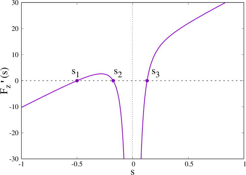
Figure 5: A plot of $F_{z}^{\prime}(s)=z+\sigma^{2}\,s-\frac{1}{2Es^{2}}$ as a function of $s$ ($s$ real) for $z=12$, $E=2$ and $\sigma^{2}=2+5E^{2}=22$. There are three zeros on the real $s$ axis (obtained by Mathematica) at $s_{1}=-0.5$, $s_{2}=-0.175186\dots$ and $s_{3}=0.129732\dots$.

We can now determine $z_{l}$ very easily. As $z$ decreases, the two negative roots $s_{1}$ and $s_{2}$ approach each other and become coincident at $z=z_{l}$ and for $z<z_{l}$, they split apart in the complex $s$ plane and become complex conjugate of each other, with their real parts identical and negative. When $s_{1}<s_{2}$, the function $F_{z}^{\prime}(s)$ has a maximum at $s_{m}$ with $s_{1}<s_{m}<s_{2}$ (see Fig. 5). As $z$ approaches $z_{l}$, $s_{1}$ and $s_{2}$ approach each other, and consequently the maximum of $F_{z}^{\prime}(s)$ between $s_{1}$ and $s_{2}$ approach the height $0$. Now, the height of the maximum of $F_{z}^{\prime}(s)$ between $s_{1}$ and $s_{2}$ can be easily evaluated. The maximum occurs at $s=s_{m}$ where $F_{z}^{\prime\prime}(s)=0$, i.e, at $s_{m}=-(E\sigma^{2})^{-1/3}$. Hence the height of the maximum is given by

$$F_{z}^{\prime}(s=s_{m})=z+\sigma^{2}\,s_{m}+\frac{1}{2s_{m}E}=z-\frac{3}{2}\left(\frac{\sigma^{4}}{E}\right)^{1/3}\,.$$ (103)

Hence, the height of the maximum becomes exactly zero when

$$z=z_{l}=\frac{3}{2}\left(\frac{\sigma^{4}}{E}\right)^{1/3}\,.$$ (104)

Thus we conclude that for $z>z_{l}$, with $z_{l}$ given exactly in Eq. (104), the function $F_{z}^{\prime}(s)$ has three real roots at $s=s_{1}<0$, $s_{2}<0$ and $s_{3}>0$, with $s_{1}$ being the smallest negative root on the real axis. For $z<z_{l}$, the pair of roots are complex (conjugates). However, it turns out (as will be shown below) that for our purpose, it is sufficient to consider evaluating the integral in Eq. (100) only in the range $z>z_{l}$ where the roots are real and evaluating the saddle point equations are considerbaly simpler. So, focusing on $z>z_{l}$, out of these $3$ roots as possible saddle points of the integrand in Eq. (100), we have to discard $s_{3}>0$ since our saddle points have to belong to the upper left quadrant of the complex $s$ plane. This leaves us with $s_{1}<0$ and $s_{2}<0$. Now, we deform our vertical contour $\Gamma_{(+)}$ by rotating it anticlockwise by $\pi/2$ so that it runs along the negative real axis. Between the two stationary points $s_{1}$ and $s_{2}$, it is easy to see (see Fig. (5)) that $F_{z}^{\prime\prime}(s_{1})>0$ (indicating that it is a minimum along real $s$ axis) and $F_{z}^{\prime\prime}(s_{2})<0$ (indicating a local maximum). Since the integral along the deformed contour is dominated by the maximum along real negative $s$ for large $N$, we should choose $s_{2}$ to be the correct root, i.e., the largest among the negative roots of the cubic equation $z+\sigma^{2}s-1/(2Es^{2})=0$.

Thus, evaluating the integral at $s^{*}=s_{2}$ (and discarding pre-exponential terms) we get for large $N$

$$I_{N}(z)\approx\exp[-N^{1/3}\chi(z)]\$$ (105)

where the rate function $\chi(z)$ is given by

$$\chi(z)=-F_{z}(s=s_{2})=-s_{2}\,z-\frac{1}{2}\sigma^{2}s_{2}^{2}-\frac{1}{2s_{2}E}$$ (106)

The right hand side can be further simplified by using the saddle point equation (102), i.e., $z+\sigma^{2}s_{2}-1/{2Es_{2}^{2}}=0$. This gives

$$\chi(z)=-\frac{zs_{2}}{2}-\frac{3}{4Es_{2}}\,.$$ (107)

B.1 Asymptotic behavior of $\chi(z)$

We now determine the asymptotic behavior of the rate function $\chi(z)$ in the range $z_{l}<z<\infty$, where $z_{l}$ is given in Eq. (104). Essentially, we need to determine $s_{2}$ (the largest among the negative roots) as a function of $z$ by solving Eq. (102), and substitute it in Eq. (107) to determine $\chi(z)$.

We first consider the limit $z\to z_{l}$ from above, where $z_{l}$ is given in Eq. (104). As $z\to z_{l}$ from above, we have already mentioned that the two negative roots $s_{1}$ and $s_{2}$ approach each other. Finally at $z=z_{l}$, we have $s_{1}=s_{2}=s_{m}$ where $s_{m}=-(E\sigma^{2})^{-1/3}$ is the location of the maximum between $s_{1}$ and $s_{2}$. Hence as $z\to z_{l}$ from above, $s_{2}\to s_{m}=-(E\sigma^{2})^{-1/3}$. Substituting this value of $s_{2}$ in Eq. (107) gives the limiting behavior

$$\chi(z)\to\frac{3}{2}\,\left(\frac{\sigma}{E}\right)^{2/3}\quad{\rm as}\,\,z\to z_{l}$$ (108)

as announced in the first line of Eq. (24).

To derive the large $z\to\infty$ behavior of $\chi(z)$ as announced in the second line of Eq. (24), it is first convenient to re-parametrize $s_{2}$ and define

$$s_{2}=-\frac{1}{\sqrt{2Ez}}\theta_{z}\,.$$ (109)

Substituting this in Eq. (102), it is easy to see that $\theta_{z}$ satisfies the cubic equation

$$-b(z)\leavevmode\nobreak\ \theta_{z}^{3}+\theta_{z}^{2}-1=0,$$ (110)

where

$$b(z)=\frac{\sigma^{2}}{\sqrt{2E}}\frac{1}{z^{3/2}}.$$ (111)

Note that due to the change of sign in going from $s_{2}$ to $\theta_{z}$, we now need to determine the smallest positive root of $\theta_{z}$ in Eq. (110). In terms of $\theta_{z}$, $\chi(z)$ in Eq. (107) reads

$$\chi(z)=\leavevmode\nobreak\ \frac{\sqrt{z}}{2\sqrt{2E}}\leavevmode\nobreak\ \frac{\theta_{z}^{2}+3}{\theta_{z}}\,.$$ (112)

The formulae in Eqs. (110), (111) and (112) are now particularly suited for the large $z$ analysis of $\chi(z)$. From Eqs. (110),(111) it follows that in the limit $z\to\infty$ we have that $b(z)\to 0$, so that $\theta_{z}\to 1$. Hence, for large $z$ or equivalently small $b(z)$, we can obtain a perturbative solution of Eq. (110). To leading order, it is easy to see that

$$\theta_{z}=1+\frac{b(z)}{2}+\mathcal{O}\left({b(z)}^{2}\right)\,.$$ (113)

with $b(z)$ given in Eq. (111). Substituting this in Eq. (112) gives the large $z$ behavior of $\chi(z)$

$$\chi(z)=\sqrt{\frac{2}{E}}\leavevmode\nobreak\ \sqrt{z}-\frac{\sigma^{2}}{4E}\frac{1}{z}+\mathcal{O}\left(\frac{1}{z^{5/2}}\right).$$ (114)

as announced in the second line of Eq. (24).

B.2 Explicit expression of $\chi(z)$

While the excercises in the previous subsections were instructive, it is also possible to obtain an explicit expression for $\chi(z)$ by solving the cubic equation (110) with Mathematica. The smallest positive root of Eq. (110), using Mathematica, reads

$$\theta_{z}=\frac{1}{3b_{z}}+\frac{1}{3\cdot 2^{2/3}b_{z}}\frac{(1-i\sqrt{3})}{\left(-2+27b_{z}^{2}+3\sqrt{-12+81b_{z}^{2}}\right)^{1/3}}+\frac{1}{3\cdot 2^{4/3}b_{z}}(1+i\sqrt{3})\left(-2+27b_{z}^{2}+3\sqrt{-12+81b_{z}^{2}}\right)^{1/3}$$ (115)

where $b_{z}$, used as an abbreviation for $b(z)$, is given in Eq. (111). Using the expression of $z_{l}$ in Eq. (104), we can re-express $b_{z}$ conveniently in a dimensionless form

$$b_{z}^{2}=\frac{1}{2}\leavevmode\nobreak\ \left(\frac{2}{3}\frac{z_{l}}{z}\right)^{3}\,.$$ (116)

Consequently, the solution $\theta_{z}$ in Eq. (115) in terms of the adimensional parameter $r=z/z_{l}\geq 1$ reads as

$$\theta_{z}\equiv\theta(r)=\frac{\sqrt{3}}{4}r^{3/2}\left[2+\frac{(1-i\sqrt{3})}{g(r)}+(1+i\sqrt{3})g(r)\right]$$ (117)

where

$$g(r)=\frac{1}{r}\left(1+i\leavevmode\nobreak\ \sqrt{r^{3}-1}\right)^{2/3}.$$ (118)

By multiplying both numerator and denominator of $\theta(r)$ by $(1-i\leavevmode\nobreak\ \sqrt{r^{3}-1})^{2/3}$ one ends up, after a little algebra, with the following expression

$$\theta(r)=\frac{\sqrt{3}}{4}r^{3/2}\left[2+\frac{1}{r}\left(\xi\leavevmode\nobreak\ \zeta_{r}^{2/3}+\overline{\xi}\leavevmode\nobreak\ \overline{\zeta}_{r}^{2/3}\right)\right],$$ (119)

where $\xi$ and $\zeta_{r}$ denotes, respectively, a complex number and a complex function of the real variable $r$:

$$\xi = 1+i\sqrt{3}$$

$$\zeta_{r} = 1+i\leavevmode\nobreak\ \sqrt{r^{3}-1},$$ (120)

and we have also introduced the related complex conjugated quantities:

$$\overline{\xi} = 1-i\sqrt{3}$$

$$\overline{\zeta}_{r} = 1-i\leavevmode\nobreak\ \sqrt{r^{3}-1},$$ (121)

We can then write the complex expressions in Eq. (119) both in their polar form, i.e., $\zeta_{r}=\rho_{r}e^{i\phi_{r}}$ and $\xi=\rho e^{i\phi}$, with, respectively:

$$\rho_{r} = r^{3/2}$$

$$\phi_{r} = \textrm{arctan}(\sqrt{r^{3}-1})$$ (122)

and

$$\rho = 2$$

$$\phi = \textrm{arctan}(\sqrt{3})=\frac{\pi}{3}.$$ (123)

Finally, by writing $\xi$ and $\zeta_{r}$ inside Eq. (119) in their polar form and taking advantage of the expressions in Eqns. (122),(123) we get:

$$\theta(r) = \frac{\sqrt{3}}{4}r^{3/2}\left[2+\frac{1}{r}\leavevmode\nobreak\ \rho\leavevmode\nobreak\ \rho_{r}^{2/3}\left(e^{i\left(\phi+\frac{2}{3}\phi_{r}\right)}+e^{-i\left(\phi+\frac{2}{3}\phi_{r}\right)}\right)\right]=$$ (124)

$$= \frac{\sqrt{3}}{2}r^{3/2}\left[1+2\cos\left(\frac{\pi}{3}+\frac{2}{3}\textrm{arctan}(\sqrt{r^{3}-1})\right)\right]$$

In order to draw explicitly the function $\chi(z)$, e.g. with the help of Mathematica, one can plug the expression of $\theta(r=z/z_{l})$ from Eq. (124) into the following formula:

$$\chi(z)=\frac{\sqrt{z}}{2\sqrt{2E}}\leavevmode\nobreak\ \frac{\theta(z/z_{l})^{2}+3}{\theta(z/z_{l})}\,,$$ (125)

B.3 The critical value $z_{c}$

We show here how to compute the critical value $z_{c}$ at which $\chi(z)$ equals $z^{2}/(2\sigma^{2})$, i.e., the value at which the two branches in Fig. 2 cross each other. To make the computations easier, it is convenient to work with dimensionless variables. Using $z_{l}=(3/2)(\sigma^{4}/E)^{1/3}$ from Eq. (104), we express $z$ in units of $z_{l}$, i.e., we define

$$r=\frac{z}{z_{l}}=\frac{2z}{3}\,\left(\frac{E}{\sigma^{4}}\right)^{1/3}\,.$$ (126)

In terms of $r$, one can rewrite $b(z)$ in Eq. (111) as (using the shorthand notation $b_{z}=b(z)$):

$$b_{z}^{2}=\frac{1}{2}\,\left(\frac{2}{3r}\right)^{3}\,.$$ (127)

Consequently, Eq. (110) reduces to

$$-\frac{1}{\sqrt{2}}\,\left(\frac{2}{3}\right)^{3/2}\,r^{-3/2}\,\theta(r)^{3}+\theta(r)^{2}-1=0\,,$$ (128)

where $\theta(r)=\theta_{z=rz_{l}}$ is dimensionless. Quite remarkably, it turns out that to determine the critical value $z_{c}$, rather conveniently we do not need to solve the above cubic equation, Eq. (128). Indeed, at $z=z_{c}$, i.e., $r=r_{c}$, equating $\chi(z_{c})=z_{c}^{2}/{2\sigma^{2}}$, we get

$$\frac{\sqrt{z_{c}}}{2\sqrt{2E}}\,\left[\frac{\theta(r_{c})^{2}+3}{\theta(r_{c})}\right]=\frac{z_{c}^{2}}{2\sigma^{2}}\,.$$ (129)

Expressing in terms of $r_{c}$, Eq. (129) simplifies to

$$\frac{\theta^{2}(r_{c})+3}{\theta(r_{c})}=\frac{3^{3/2}}{2}\,r_{c}^{3/2}\,.$$ (130)

Consider now Eq. (128) evaluated at $r=r_{c}$. In this equation, we replace $r_{c}$ by its expression in Eq. (130). This immediately gives $\theta(r_{c})^{2}=3/2$ and hence

$$\theta(r_{c})=\sqrt{\frac{3}{2}}\,.$$ (131)

Using this exact $\theta(r_{c})$ in Eq. (130) gives

$$r_{c}=\frac{z_{c}}{z_{l}}=2^{1/3}=1.25992\dots$$ (132)

It is now straightforward to check that the expression of $\theta(r)$ written in Eq. (124) is consistent with the result just found, i.e., from it we retrieve $\theta(r_{c}=2^{1/3})=\sqrt{3/2}$. We have that

$$\theta(r_{c}=2^{1/3}) = \frac{\sqrt{3}}{2}r_{c}^{3/2}\left[1+2\cos\left(\frac{\pi}{3}+\frac{2}{3}\textrm{arctan}(\sqrt{r_{c}^{3}-1})\right)\right]=$$ (133)

$$= \sqrt{\frac{3}{2}}\left[1+2\cos\left(\frac{\pi}{3}+\frac{2}{3}\textrm{arctan}(1)\right)\right]=\sqrt{\frac{3}{2}}\left[1+2\cos\left(\frac{\pi}{2}\right)\right]=$$

$$= \sqrt{\frac{3}{2}},$$

as expected.

For comparison to numerical simulations, we chose $E=2$, for which $\sigma^{2}=2+5E^{2}=22$. We get $z_{l}=(3/2)(\sigma^{4}/E)^{1/3}=9.34752\ldots$, which gives $z_{c}=r_{c}z_{l}=(1.25992\dots)z_{l}=11.7771\dots.$ This is represented by a black dotted vertical line in Fig. 4.

References

- [1] M.C. Marchetti, J.F. Joanny, S. Ramaswamy, T.B. Liverpool, J. Prost, M. Rao, A. Simha, Rev. Mod. Phys. 85, 1143 (2013).
- [2] C. Bechinger, R. Di Leonardo, H. Lowen, C. Reichhardt, G. Volpe, G. Volpe, Rev. Mod. Phys. 88, 045006 (2016).
- [3] S. Ramaswamy, J. Stat. Mech. P054002 (2017).
- [4] E. Fodor, M. C. Marchetti, Physica A 504, 106 (2018).
- [5] J. Tailleur, M. E. Cates, Phys. Rev. Lett. 100, 218103 (2008).
- [6] Y. Fily, M.-C. Marchetti, Phys. Rev. Lett. 108, 235702 (2012).
- [7] I. Buttinoni, J. Bialké, F. Kümmel, H. Löwen, C. Bechinger, T. Speck, Phys. Rev. Lett. 110, 238301 (2013).
- [8] M. E. Cates, J. Tailleur, Europhys. Lett. 101, 20010 (2013).
- [9] M. E. Cates, J. Tailleur, Annu. Rev. Condens. Matter Phys. 6, 219-244 (2015).
- [10] A. P. Solon, M. E. Cates, J. Tailleur, Eur. Phys. J. Special Topics 224, 1231-1262 (2015).
- [11] H.C. Berg, “E. coli in Motion”, Springer, New York (2003).
- [12] A.B. Slowman, M.R. Evans, R.A. Blythe, Phys. Rev. Lett. 116 218101 (2016).
- [13] J. Stenhammar, R. Wittkowski, D. Marenduzzo, M. E. Cates, Phys. Rev. Lett. 114, 018301 (2015).
- [14] F. J. Sevilla and L. A. Gomez Nava, Phys. Rev. E 90, 022130 (2014).
- [15] F. J. Sevilla and M. Sandoval, Phys. Rev. E 91, 052150 (2015).
- [16] S.C. Takatori, R. De Dier, J. Vermant, and J. F. Brady, Nat. Commun., 7, 10694 (2016).
- [17] C. Kurzthaler, C. Devailly, J. Arlt, T. Franosch, W.C.K. Poon, V.A. Martinez, and A.T. Brown, Phys. Rev. Lett. 121, 078001 (2018).
- [18] U. Basu, S. N. Majumdar, A. Rosso, and G. Schehr, Phys. Rev. E 98, 062121 (2018).
- [19] O. Dauchot and V. Demery, arXiv: 1810.13303
- [20] K. Malakar, A. Das, A. Kundu, K. Vijay Kumar, and A. Dhar, arXiv: 1902.04171
- [21] J. Masoliver and K. Lindenberg, Eur. Phys. J B 90, 107 (2017).
- [22] G. H. Weiss, Physica A: Statistical Mechanics and its Applications, bf 311, 381 (2002).
- [23] L. Angelani, R. Di Lionardo, and M. Paoluzzi, Euro. J. Phys. E 37, 59 (2014).
- [24] L. Angelani, J. Phys. A: Math. Theor. bf 48, 495003 (2015).
- [25] K. Malakar, V. Jemseena, A. Kundu, K. Vijay Kumar, S. Sabhapandit, S. N. Majumdar, S. Redner, A. Dhar, J. Stat. Mech. P043215 (2018).
- [26] T. Demaerel and C. Maes, Phys. Rev. E 97, 032604 (2018).
- [27] M. R. Evans and S. N. Majumdar, J. Phys. A: Math. Theor. 51, 475003 (2018).
- [28] P. Le Doussal, S. N. Majumdar, and G. Schehr, arXiv: 1902.06176
- [29] A. Dhar, A. Kundu, S. N. Majumdar, S. Sabhapandit, G. Schehr, Run-and-tumble particle in one-dimensional confining potential: Steady state, relaxation and first passage properties, arXiv: 1811.03808, to appear in Phys. Rev. E (2019).
- [30] S. N. Majumdar, M. R. Evans, R. K. P. Zia, Phys. Rev. Lett. 94, 180601 (2005).
- [31] M. R. Evans, S. N. Majumdar, R. K. P. Zia, J. Stat. Phys. 123, 357 (2006).
- [32] M. R. Evans, T. Hanney, J. Phys. A: Math. Gen. 38, R195 (2005).
- [33] S.N. Majumdar, “Real-space Condensation in Stochastic Mass Transport Models”, Les Houches lecture notes for the summer school on “Exact Methods in Low-dimensional Statistical Physics and Quantum Computing” (Les Houches, July 2008), ed. by J. Jacobsen, S. Ouvry, V. Pasquier, D. Serban and L.F. Cugliandolo, Oxford University Press.
- [34] J. Szavits-Nossan, M. R. Evans, S. N. Majumdar, Phys. Rev. Lett. 112, 020602 (2014).
- [35] J. Szavits-Nossan, M. R. Evans, S. N. Majumdar, J. Phys. A: Math. Theor. 47, 455004 (2014).
- [36] J. Szavits-Nossan, M. R. Evans, S. N. Majumdar, J. Phys. A: Math. Theor. 50, 024005 (2017).
- [37] G. Gradenigo, E. Bertin, Entropy 19, 517 (2017).
- [38] G. Gradenigo, A. Sarracino, A. Puglisi, H. Touchette, J. Phys. A: Math. Theor. 46, 335002 (2013).
- [39] A. V. Nagaev, Theor. Probab. Appl. 14, 51 (1969); 14, 193 (1969).
-
[40]
The general formula for the saddle-point
approximation of a contour integral in the complex plane which
depend on a large parameter is
(134) - [41] P. Dennery, A. Krzywicki, “Mathematics for Physicists”, Harper & Row, New York (1967).
- [42] P. Vivo, S. N. Majumdar, O. Bohigas, Phys. Rev. Lett. 101, 216809 (2008).
- [43] S. N. Majumdar, C. Nadal, A. Scardicchio, and P. Vivo, Phys. Rev. Lett. 103, 220603 (2009).
- [44] P. Vivo, S. N. Majumdar, O. Bohigas, Phys. Rev. B 81, 104202 (2010).
- [45] C. Nadal, S. N. Majumdar, M. Vergassola, Phys. Rev. Lett. 104, 110501 (2010).
- [46] C. Nadal, S. N. Majumdar, M. Vergassola, J. Stat. Phys., 142, 403-438 (2011).
- [47] S. N. Majumdar, C. Nadal, A. Scardicchio, and P. Vivo, Phys. Rev. E 83, 041105 (2011).
- [48] C. Texier and S. N. Majumdar, Phys. Rev. Lett. 110, 250602 (2013).
- [49] S. N. Majumdar, G. Schehr, J. Stat. Mech. P01012 (2014).
- [50] F. D. Cunden, F. Mezzadri, and P. Vivo, J. Stat. Phys. 164, 1062 (2016).
- [51] F. D. Cunden, P. Facchi, M. Ligabo, and P. Vivo, J. Stat. Mech. 053303 (2017).
- [52] A. Grabsch, S. N. Majumdar, C. Texier, J. Stat. Phys. 167, 234 (2017).
- [53] B. Lacroix-A-Chez-Toine, A. Grabsch, S. N. Majumdar, and G. Schehr, J. Stat. Mech. 013203 (2018).
- [54] G. Gradenigo and S. N. Majumdar, “A free Run-and-Tumble particle and the first-order transition in the space of its trajectories.”, in preparation.
- [55] G. Gradenigo, S. Iubini, R. Livi and S. N. Majumdar, “Localization in the Discrete Non-Linear Schrödinger Equation: mechanism of a First-Order Transition in the Microcanonical Ensemble”, in preparation.
- [56] G. Gradenigo, U. Marini Bettolo Marconi, A. Puglisi, A. Sarracino, Phys. Rev. E 85, 031112 (2012).
- [57] A. Gervois, J. Piasecki, J. Stat. Phys. 42, 1091 (1986).
- [58] A. Alastuey, J. Piasecki, J. Stat. Phys. 139, 991 (2010).
- [59] K. Martens, L. Angelani, R. Di Leonardo, L. Bocquet Probability distributions for the run-and-tumble bacterial dynamics: An analogy to the Lorentz model Eur. Phys. J. E 35, 84 (2012).