Warm CO in evolved stars from the THROES catalogue

Abstract

Context. This is the second paper of a series making use of Herschel/PACS spectroscopy of evolved stars in the THROES catalogue to study the inner warm regions of their circumstellar envelopes (CSEs).

Aims. We analyze the CO emission spectra, including a large number of high-$J$ CO lines (from $J$=14-13 to $J$=45-44, $\nu$=0), as a proxy for the warm molecular gas in the CSEs of a sample of bright carbon-rich stars spanning different evolutionary stages from the Asymptotic Giant Branch (AGB) to the young planetary nebulae (PNe) phase.

Methods. We use the rotational diagram (RD) technique to derive rotational temperatures ($T_{\rm rot}$) and masses ($M_{\rm H_{2}}$) of the envelope layers where the CO transitions observed with PACS arise. Additionally, we obtain a first order estimate of the mass-loss rates and assess the impact of the opacity correction for a range of envelope characteristic radii. We use multi-epoch spectra for the well studied C-rich envelope IRC+10216 to investigate the impact of CO flux variability on the values of $T_{\rm rot}$ and $M_{\rm H_{2}}$.

Results. PACS sensitivity allowed the study of higher rotational numbers than before indicating the presence of a significant amount of warmer gas ($\sim$200-900 K) not traceable with lower-$J$ CO observations at sub-mm/mm wavelengths. The masses are in the range $M_{\rm H_{2}}$$\sim 10^{-2}-10^{-5}\,\rm M_{\sun}$, anti-correlated with temperature. For some strong CO emitters we infer a double temperature (warm $\overline{T}_{\rm rot}\sim$400 K and hot $\overline{T}_{\rm rot}\sim$820 K) component. From the analysis of IRC+10216, we corroborate that the effect of line variability is perceptible on the $T_{\rm rot}$ of the hot component only, and certainly insignificant on $M_{\rm H_{2}}$ and, hence, the mass-loss rate. The agreement between our mass-loss rates and the literature across the sample is good. Therefore, the parameters derived from the RD are robust even when strong line flux variability occurs, with the major source of uncertainty in the estimate of the mass-loss rate being the size of the CO-emitting volume.

1 Introduction

The asymptotic giant branch (AGB) is a late evolutionary stage of low-to-intermediate mass stars (1 $\rm M_{\sun}$$\la$M_⋆$\la$8$\rm M_{\sun}$) which is largely dominated by mass-loss processes. AGB stars can shed significant portions of their outer atmospheric layers in a dust-driven wind, with mass-loss rates of up to $\dot{M}$$\sim$10${}^{-4}\rm\,M_{\sun}\,yr^{-1}$ (e.g. Habing 1996; Höfner & Olofsson 2018). The material expelled by the central star (with very low effective temperatures of $T_{\rm eff}$$\sim$2000-3000 K) forms a cool, dense circumstellar envelope (CSE) that is rich in dust grains and a large variety of molecules. After a significant decrease of the mass-loss rate, the AGB phase ends and the ‘star+CSE’ system begins to evolve to the Planetary Nebula (PN) phase, at which the CSE is fully or almost fully ionized due to the much higher central star temperatures ($T_{\rm eff}$$\approx$10⁴-10⁵ K) and more diluted envelopes. During the AGB-to-PN transition, shocks – resulting from the interaction between slow and fast winds at the end of the AGB phase (or early post-AGB) – also play an important role changing the morphology, dynamics and chemistry of the CSEs (e.g. Kwok 2000; van Winckel 2003; Bujarrabal 2006).

The CO molecule is an excellent tracer of the CSEs of AGB stars, post-AGB objects and PNe (e.g Groenewegen et al. 1996; Schöier & Olofsson 2001; Schöier et al. 2002; Teyssier et al. 2006). The rotational transitions of the ground vibrational level over a wide range of excitation energies sample from cold ($\sim$10 K) to hot gas ($\sim$1000 K). Literature on observations of the cold, extended CO $J=1-0$ to $J=6-5$ emission around many evolved stars is abundant at mm/sub-mm wavelengths (e.g. Knapp et al. 1982; Knapp & Morris 1985; Knapp & Chang 1985; Olofsson et al. 1993; Bujarrabal et al. 1989; Jorissen & Knapp 1998; Castro-Carrizo et al. 2010; Sánchez Contreras & Sahai 2012; Ramstedt & Olofsson 2014). Studies looking at far-infrared (FIR) observations of even higher $J$ CO transitions probing the warmest gas ($\sim$200-1000 K) in deeper layers of CSEs are much more scarce. Pioneering works based on observations with the Infrared Space Observatory ($ISO$) (e.g. Justtanont et al. 2000; Schöier et al. 2002) have continued more recently with Herschel (e.g. Groenewegen et al. 2011; Bujarrabal et al. 2012; Khouri et al. 2014; Danilovich et al. 2015; Nicolaes et al. 2018).

This is the second of a series of papers (Ramos-Medina et al. 2018a, Paper I) where we analyze in an uniform and systematic way Herschel/PACS spectra of a large sample of evolved stars from the THROES catalogue (Ramos-Medina et al. 2018b) to study their warm inner envelope regions using high-$J$ CO transitions at FIR wavelengths. As in other previous studies, we divide our sample in O-rich and C-rich targets (papers I and II, respectively) since these two major chemistry classes correspond to progenitor stars with different masses, which follow somewhat different evolutionary paths, and also have a dissimilar dust composition, both facts potentially affecting the mass-loss process. We include targets with different evolutionary stages: AGB, post-AGB (or pre-PNe) and young planetary nebulae (yPNe).

The goal of our study (papers I and II) is to obtain a first estimate of the average excitation temperature ($T_{\rm rot}$) and mass ($M_{\rm H_{2}}$) of the warm envelope layers traced by the PACS CO lines in a uniform way using a simple analysis technique, the well-known rotational diagram (RD) method. The RD technique is useful to rapidly analyze large data sets (large number of lines and/or large samples) and to provide some constraints on these fundamental parameters. With the aim of benchmarking the results of the RD approximation, we obtain rough estimates of mass-loss rates ($\dot{M}$) and compare them to values in the literature, paying particular attention to studies including at least a few high-$J$ CO (FIR) transitions.

The impact of possible non-LTE effects on the results from the simple RD analysis was investigated in paper I. It was concluded that, though they are expected to be minor in general and probably only affecting the highest-$J$ CO transitions studied here ($J$$\ga$27) at most, their existence cannot be ruled out in the lowest mass-loss rate stars and/or the outermost layers of the PACS CO-emitting volume. We also showed that even under non-LTE conditions, the masses derived from the RDs are approximately correct (or, at the very least, not affected by unusually large uncertainties) since the average excitation temperature describes rather precisely the molecular excitation (i.e., the real level population). This is also corroborated by the good agreement found between our estimates of $\dot{M}$ and those from detailed non-LTE excitation and radiative transfer (nLTEexRT) studies that exist for a number of targets. We stress that the RD method enables a characterization of the warm CSEs of evolved stars in a first approximation and that for a more robust and detailed study of the radial structure of the density, temperature and velocity in the CSEs, as well as for establishing potential mass-loss rate variations with time, more sophisticated analysis is needed (e.g., Ryde et al. 1999; Schöier et al. 2002; De Beck et al. 2012).

Upon submission of this manuscript (and after our paper I was accepted for publication) we became aware of a recent work by Nicolaes et al. (2018) who independently presented Herchel/PACS (and SPIRE) range spectroscopy of a sample of 37 AGB stars. These authors perform a similar RD analysis of the CO spectra and focus on deriving excitation temperatures (in contrast to our study, estimates of the envelope mass or mass-loss rates are not reported). Other differences with respect to the work by Nicolaes et al. (2018) is that we introduce a canonical opacity correction in the RDs and that we include post-AGBs and PNe.

2 Observations

2.1 Observations and data reduction

PACS is a photometer and medium resolution grating spectrometer (Poglitsch et al. 2010) onboard the Herschel Space Telescope (Pilbratt et al. 2010) probing the FIR wavelength range. The PACS spectrometer covers the wavelength range from 51 to 210 $\mu$m in two different channels that operate simultaneously in the blue (51-105 $\mu$m) and red (102-220 $\mu$m) bands. The Field of View (FoV) covers a 47″$\times$47″ region in the sky, structured in an array of 5$\times$5 spatial pixels (”spaxels”) with 9.4″$\times$9.4″. PACS provides a resolving power between 5500 and 940, i.e. a spectral resolution of approximately 55-320 $\rm km\leavevmode\nobreak\ s^{-1}$, at short and long wavelengths, respectively, and the PSF of the PACS spectrometer ranges from $\sim$ 9″ in the blue band to $\sim$13″ in the red band. The PSF is described in da Silva Santos (2016) and Bocchio et al. (2016). The technical details of the instrument can be found in the PACS Observer’s Manual.

The PACS (1D) spectral data were taken from the THROES (caTalogue of HeRschel Observations of Evolved Stars) website which contains fully reduced PACS spectra of a collection of 114 stars, mostly low-to-intermediate mass AGB stars, post-AGB and PNe. The data reduction is explained in Ramos-Medina et al. (2018b) in full detail. The catalogue also consists of a compilation of previous photometry measurements at 12, 25, 60, 100 $\rm\mu m$ with the Infrared Astronomical Satellite (IRAS).

Table 3 offers a description of the observations used here where we provide the target name as listed in the header of the PACS FITS files and an alternative name for which some of the stars are more well known in the literature. We only analyzed the spectra between [55-95] and [101-190] $\rm\mu m$ because the flux densities are unreliable above 190 $\rm\mu m$, below 55 $\rm\mu m$ and between 95-101 $\rm\mu m$ due to spectral leakage. Two observation identifiers (OBSIDs) per target, corresponding to the bands B2A, B2B and R1, are necessary to cover the full PACS wavelength range. In the case of IRC+10216, band B2A data exists (see Decin et al. 2010), but these were acquired in a non-standard spectroscopy mode and have restricted access in the Herschel Science Archive and, thus, are not included in the THROES catalogue. Instead, we used 4+3 OBSIDs corresponding to seven different operational days: OD = [745, 1087, 1257 and 1296] covering the spectral range [69-95, 140-190] $\rm\mu m$ and OD = [894, 1113 and 1288] covering a narrower interval [77-95, 155-190] $\rm\mu m$.

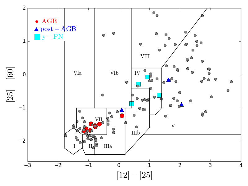
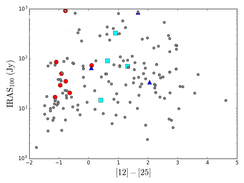
Figure 1: IRAS color diagrams for the stars in the THROES catalogue. The colors are defined from the infrared fluxes at 12, 25 and 60 $\rm\mu m$. The boxes on the left panel are the ones defined in van der Veen & Habing (1988), and the highlighted points correspond to the stars studied in this paper.

2.2 Sample overview

We searched for CO emission amongst the entire THROES catalog, but in this paper we focus on C-rich CSEs (29% of the entries) observed in PACS range mode. We found 15 evolved stars with at least three CO emission lines with signal-to-noise ratio above 3.

This sample contains bright infrared targets spanning a range of evolutionary stages from the AGB to the PN phase, but sharing similar carbon chemistry with strong CO emission at high excitation temperatures (up to $E_{\rm u}/k\approx 5688$ K). The AGBs, which are mostly Mira variables, are known for their high mass-loss rates compared to the mean value of $\dot{M}\sim 1.5\times 10^{-7}\rm\leavevmode\nobreak\ M_{\sun}\leavevmode\nobreak\ yr^{-1}$ derived from studies with large samples of carbon stars (Olofsson et al. 1993). We also include two mixed-chemistry post-AGBs (Red Rectangle and IRAS 16594-4656, Waters et al. 1998; Woods et al. 2005) and two mixed-chemistry yPNes (Hen 2-113 and CPD-56°8032, De Marco & Crowther 1998; Danehkar & Parker 2015, and references therein), that is, they show both C-rich and O-rich dust grains. In the Appendix we provide Table 4 with a summary of some relevant properties such as distance, effective temperature and gas mass-loss rate, along with additional references.

Figure 1 shows the classic IRAS color-color diagram (van der Veen & Habing 1988) featuring the colors $[25]-[60]=-2.5\log\frac{IRAS_{25}}{IRAS_{60}}$ and $[12]-[25]=-2.5\log\frac{IRAS_{12}}{IRAS_{25}}$ of all the stars in THROES. The stars here studied are highlighted with colored filled symbols which we will use consistently throughout the paper. This diagram is known to be a good indicator of the evolutionary stage of low-to-intermediate evolved stars, with AGBs populating the lower left corner and more advanced stages being located on the diametrically opposed, so-called cold, side of the diagram. It also shows an evolution in terms of the mass-loss rate and/or progressively increasing optical depths (Bedijn 1987). C-rich AGBs clearly constellate in a different box compared to the O-rich stars in Paper I, which has been interpreted as a consequence of different grains’ emissivities (Zuckerman & Dyck 1986). The AGB star that falls outside the expected box with a clear 25 $\rm\mu m$ excess ($[12]-[25]=0.1$) is AFGL 3068 (LL Peg), which is an ”extreme carbon star”: very dust-obscured by optically thick shells due to high mass-loss rate (Volk et al. 1992; Winters et al. 1997). The post-AGB object HD 44179, best known as The Red Rectangle, is also outlying in this same box with respect to objects in a similar evolutionary status beyond the AGB, which typically show much larger 25 $\rm\mu m$ excess indicative of detached cold dust (and gas) envelopes.

3 Observational results

3.1 Features in PACS spectra

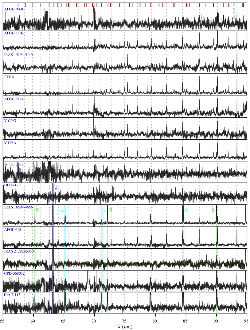
Figure 2: Continuum-subtracted PACS spectra of our sample. The vertical segments (at the top) and bars indicate the rotational transitions of $\rm{}^{12}CO$ (light gray, dotted lines), $\rm{}^{13}CO$ (dark gray), HCN (red), CS (yellow), OH (cyan), $\rm CH^{+}$ (green) and forbidden lines (blue) of [C II] $157.7\,\rm\mu m$, [O I] $63.2,145.5\,\rm\mu m$, [N II] $121.9\,\rm\mu m$.

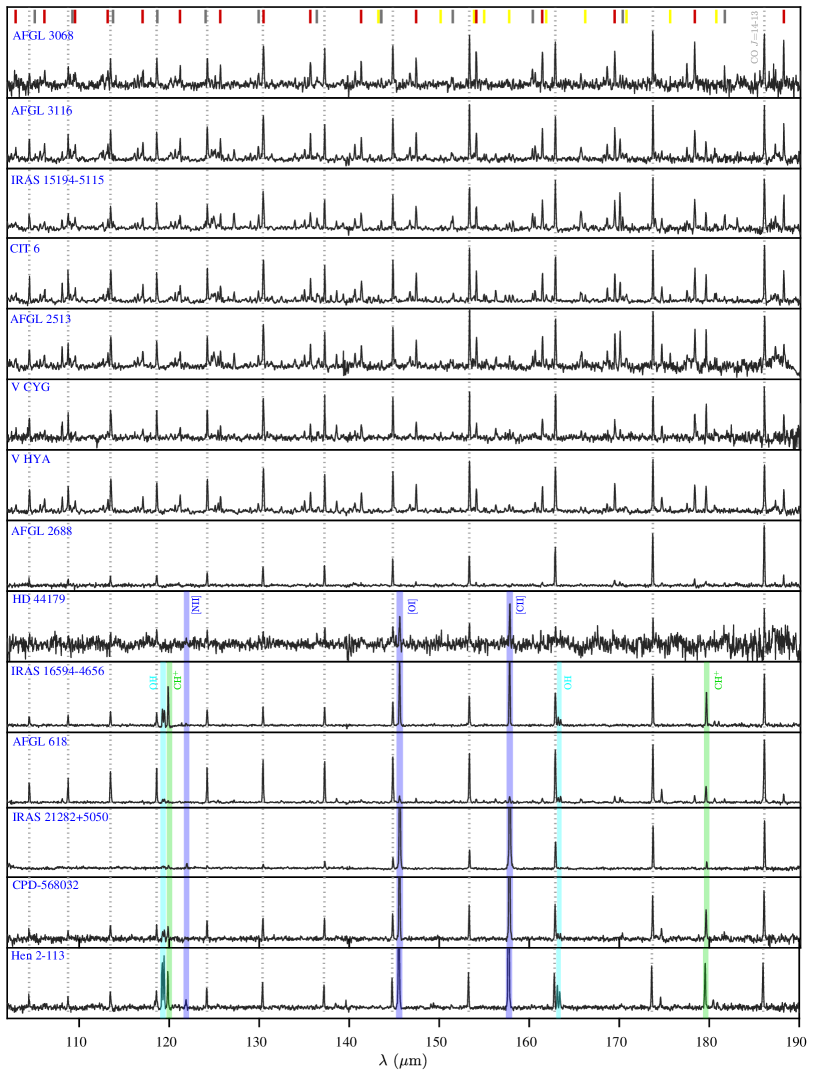
Figure 3: Continued.

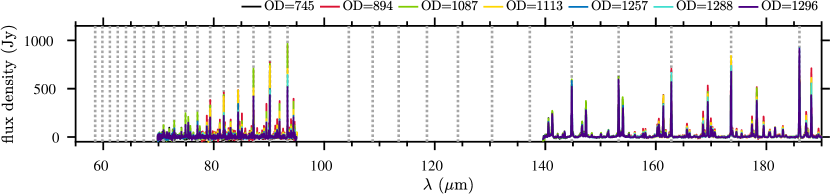
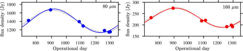
Figure 4: Line and continuum variability of IRC+10216 in the FIR. Top: Continuum subtracted spectra at different epochs (see also Fig. 18); the dotted lines sign the CO transitions. Bottom: Sine-wave fit to the continuum variability at two selected wavelengths for a fixed pulsation period of 630 days (solid lines) and free-period fit corresponding to 680 and 660 days for the blue and red dashed curves, respectively.

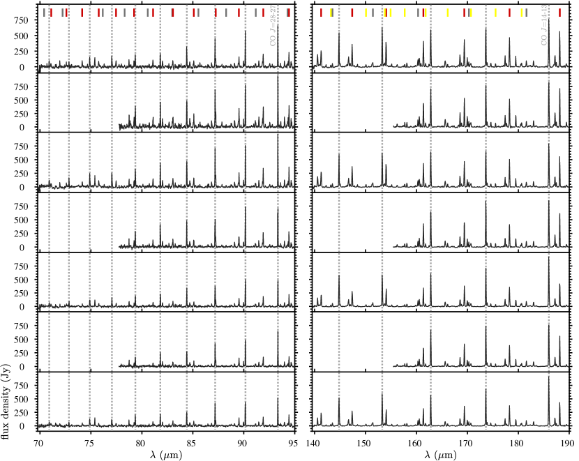
Figure 18: Spectra of IRC+10216 at different epochs. Each row corresponds to a different observing day (from top to bottom: OD = 745, 894, 1087, 1113, 1257, 1288, 1296). Same color code for the top tick marks as in Fig.2.

The PACS continuum-subtracted spectra are plotted in Fig. 2 sorted in terms of stellar effective temperature ($T_{\rm eff}$ increases from top to bottom) and arbitrarily scaled for better comparison of the CO spectra. The continuum was fitted using a non-parametric method after identifying the line-free regions of the spectrum for each target. A brief line-detection statistics summary is given in Table 5. Broad emission or absorption features due to instrumental artifacts are occasionally visible in some of the targets (e.g. near 62 $\rm\mu m$). The spectra of IRC+10216 taken at seven different epochs are shown in the top panel of Fig. 4, and in more detail in Fig. 18 in the Appendix.

Straightaway we see significant differences between the spectra of these targets such as the larger line density, resulting from a richer molecular content, in AGB stars compared to post-AGBs and yPNe as expected. In AGB stars the strongest spectral lines are due to CO emission, while post-AGBs and yPNe show much more prominent forbidden lines, except for AFGL 2688 and AFGL 618. Additional molecular features with intense emission are attributed to rotational transitions of common C-bearing species such as ¹³CO, HCN, CS, etc.

Not so common in C-rich stars is the presence of OH, yet we identify several OH doublet lines (at 79, 84, 119 and 163 $\mu$m) in all yPNe and in the post-AGB star IRAS 16594-4656, with the highest $T_{\rm eff}$$\sim$10 000K in its class and where the presence of shocks is plausible. Two additional OH doublets at 65 and 71 $\mu$m, with high-excitation energy of about 500 and 600 K, respectively, are also observed in IRAS 16594-4656 and in the yPNe Hen 2-113. In those five ($T_{\rm eff}$$>$10 000 K) targets, we also identify pure rotational transitions of CH⁺, with the $J$=3-2 line at 119.86 $\mu$m being one of the most clearly detected and best isolated lines. The 179.61 $\mu$m CH⁺ line could be blended with the water 2₁₂-1₀₁ transition. The highest-$J$ lines of CH⁺ are also present in IRAS 16594-4656 and Hen 2-113. Interestingly, we do not see CH⁺ in the spectrum of the Red Rectangle, where sharp emission features near 4225 Å were discovered and assigned to this ion by Balm & Jura (1992). The detection of CH⁺ in AFGL 618 and the more evolved PNe NGC 7027 had been previously reported by Wesson et al. (2010, Herschel/SPIRE) and Cernicharo et al. (1997, ISO data). As we see below in this section, the targets with CH⁺ and OH emission also show the strongest atomic/ionic fine-structure lines.

We identify lines due to $\rm H_{2}O$ (orto- and para-) transitions in all AGBs, in the post-AGB AFGL 2688 and in the yPNe AFGL 618. The study of water lines in the C-rich AGB stars of our sample (except for AFGL 2513) was already conducted by Lombaert et al. (2016) who suggested that both shocks and UV photodissociation may play a role in warm $\rm H_{2}O$ formation. Water lines had also been previously identified in the SPIRE spectrum of AFGL 618 and AFGL 2688 Wesson et al. (2010).

The fine-structure lines [O I] at 63.18 $\rm\mu m$ and 145.53 $\rm\mu m$ and [C II] at 157.74 $\rm\mu m$ are very prominent in the spectra of all post-AGBs and yPNe in our sample with the exception of AFGL 2688. The post-AGB object IRAS 16594-4656 demonstrates clear signs of ionization since it shows a [C II] line even stronger than that of AFGL 618, which has a hotter central star (Table B.1). Weak [N II] 121.89 $\rm\mu m$ emission is also detected in Hen 2-113 and IRAS 21282+5050, and, tentatively in IRAS 16594-4656 and HD 44179.

The 69 $\rm\mu m$ band of forsterite (Mg₂SiO₄) is visible in  CPD-$56^{\circ}8032$, Hen 2-113, and HD 44179, as already reported by Cohen et al. (2002) and Blommaert et al. (2014). The presence of O-rich dust in such C-rich objects corroborates a mixed chemistry nature.

3.2 Line flux variability in IRC+10216

Variability of the continuum at optical and IR wavelengths due to stellar pulsations is a common property of AGB stars. We present PACS spectra at multiple epochs of the Mira-type C-rich star IRC+10216 displaying periodic variations both in the continuum and in the lines (see Fig. 4 and Fig. 18).

Cernicharo et al. (2014) first reported on the discovery of strong intensity variations in high-excitation lines of abundant molecular species towards IRC+10216 using Herschel/HIFI and IRAM 30m data. Line variability was attributed to periodic changes in the IR pumping rates and also possibly in the dust and gas temperatures in the innermost layers of the CSE. From the analysis of a 3 yr-long monitoring of the molecular emission of IRC+10216 with Herschel (including HIFI, SPIRE and PACS data), Teyssier et al. (2015) concluded that intensity changes of CO lines with rotational numbers up to $J$=18 are within the typical instrument calibration uncertainties, but in the higher PACS frequency range ($J\geq 28$), line strength variations of a factor $\ga$1.6, and scaling with $J$, were found. More recently, He et al. (2017) reported 5%-30% intensity variability of additional mm lines with periodicities in the range 450-1180 days.

In section 5.3 we study in greater detail what is the impact of CO line variability on the estimate of $T_{\rm rot}$ and $M_{\rm H_{2}}$ from the rotational diagram analysis using PACS data for different epochs.

3.3 CO line fluxes

We now focus on the purely rotational spectrum of CO in the ground vibrational state ($v$=0), which we use to study the physical properties of the warm regions of the molecular CSEs of our targets. In the PACS range one can potentially find very high CO rotational transitions, from $J=14-13$ ($E_{\rm u}$$\sim$581 K) to $J=45-44$ ($E_{\rm u}$$\sim$5688 K). The lack of data between 95 and 101 $\rm\mu m$ means we cannot detect the transitions $J$=26-25 and $J$=27-26. In the case of IRC +10216, the much larger gap in the PACS coverage ($\sim$95-140 $\mu$m, Fig. 4) prevents detection of CO transitions with upper-level rotational number between $J_{\rm u}$=19 and $J_{\rm u}$=27.

The line fluxes are given in Table 6. The quoted uncertainties correspond to the propagated statistical errors and do not contain absolute flux calibration errors (typically of $\sim$15%-20%) or underlying continuum subtraction uncertainties.

As expected, the resolving power of PACS ($\sim$80-300 km s^-1) does not allow to spectrally resolve the CO profiles. This is true not only for AGB CSEs with full-widths-at-half-maximum (FWHM) similar to or smaller than the terminal expansion velocity of the envelopes (FWHM$\sim$10-25 km s^-1, Table 4), but also for post-AGB objects and yPNe, even in targets that are known to have fast ($\approx$100 km s^-1) molecular outflows like AFGL 618 (e.g. Bujarrabal et al. 2010). For this reason we measured CO fluxes by simply fitting a Gaussian function to the PACS lines.

Due to insufficient spectral resolution some reported line fluxes are affected by line blend. These are identified with asterisks in the tables and figures. Some of the well-known line blends are CO $J$=30-29 with HCN $J$=39-38 and CO $J$=20-19 with HCN $J$=26-25 at 87.2 and 130.4 $\mu$m, respectively. Also, the CO transitions $J$=21-20 and $J$=22-21 are blended with ¹³CO $J$=22-21 and $J$=23-22 at $124.2\leavevmode\nobreak\ \rm\mu m$ and $118.6\leavevmode\nobreak\ \rm\mu m$, respectively.

Figure 5 compares the integrated flux of the CO ($J$=15-14) line ($F_{\rm CO\,(15-14)}$) with the IRAS 100 $\mu$m flux (IRAS₁₀₀), the PACS continuum at 170 $\mu$m (PACS₁₇₀), i.e.  near the CO ($J$=15-14) line, and the [12]-[25] IRAS color. The $J$=15-14 transition is a strong, non-blended line, detected towards all of our targets, and it was also used by Lombaert et al. (2016) who analyzed PACS data of most of the AGBs here studied, which facilitates comparison.

As for the O-rich sample (paper I), there is a positive correlation between the CO line strength and the IRAS₁₀₀ and PACS₁₇₀ continuum fluxes. The correlation between the CO $J$=1-0 line and the IRAS fluxes of evolved stars of various chemical types had been previously reported (Olofsson et al. 1987, 1988; Bujarrabal et al. 1992). We also confirm the anticorrelation between the line-to-continuum ($F_{\rm CO\ 15-14}$/PACS₁₇₀) ratio and the IRAS [12]-[25] color (both distance-independent) for the AGB stars, which was noted in Paper I. For the more evolved targets the trend is not so obvious, but the sample size is small. We also see that, in general, the ratio between the molecular emission and the dust emission is higher in less evolved objects than in the most evolved ones, which could be partially attributed to more prominent CO photodissociation as the objects evolves along the AGB-to-PNe track. AFGL 618 and IRAS 16594-4656 are two clear outliers in this relation since they show a line-to-continuum emission ratio as large as that of the AGB class. The Red Rectangle (HD 44179) is well isolated in all the panels due to its comparatively weak CO emission and low CO-to-dust ratio. This surely reflects the different nature of this object with respect to the rest of post-AGB and yPNe in our sample, which is well known from previous works. The Red Rectangle belongs to a special class of post-AGB objects with relatively weak CO emission coming from large ($\sim$1000-2000 AU) circumbinary rotating disks, with very prominent IR emission by warm/hot dust in the disk, but lacking massive molecular outflows found in many other evolved stars (e.g., Bujarrabal et al. 2016, and references therein).

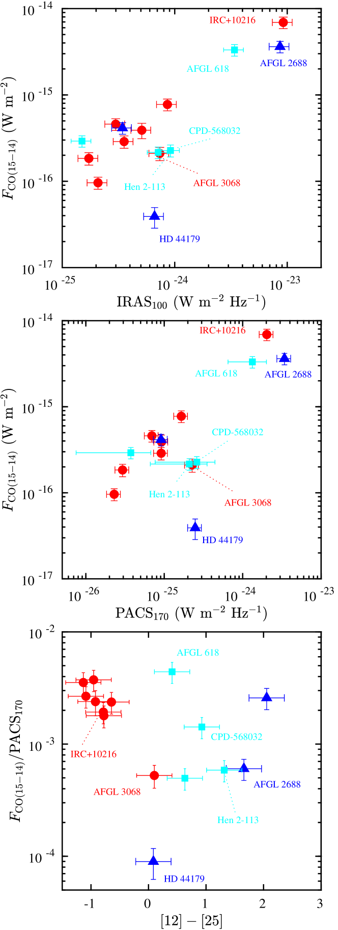
Figure 5: Correlation between CO line flux and continuum intensities. Top: CO $J=15-14$ vs IRAS 100 $\rm\mu m$ flux. Middle: CO $J=15-14$ vs PACS 170 $\rm\mu m$ continuum flux. Bottom: continuum normalized CO $J=15-14$ flux vs IRAS [12]-[25] color. The symbols and colors are the same as in Fig. 1.

4 Rotational diagram analysis

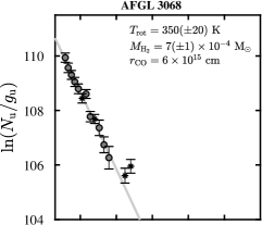
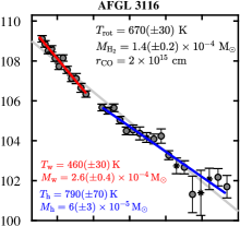
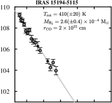
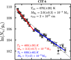
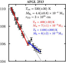
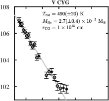
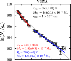
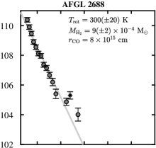
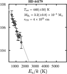
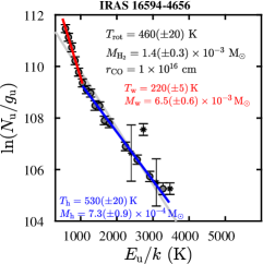
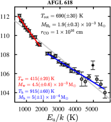
Figure 6: Rotational diagrams of the CO molecule. The gray line correspond to a single least-squares fit to the full range of transitions from where a rotational temperature, $T_{\rm rot}$, and total gas mass, $M_{\rm H_{2}}$, is computed. The characteristic radius of the CO-emitting volume ($r_{\rm CO}$) adopted is indicated. The red and blue lines correspond to a two-component model consisting of a ”warm” and ”hot” region, respectively. Asterisks mark line blends that were excluded in the fit.

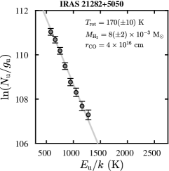
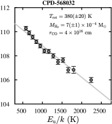
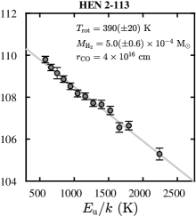
Figure 7: Continued.

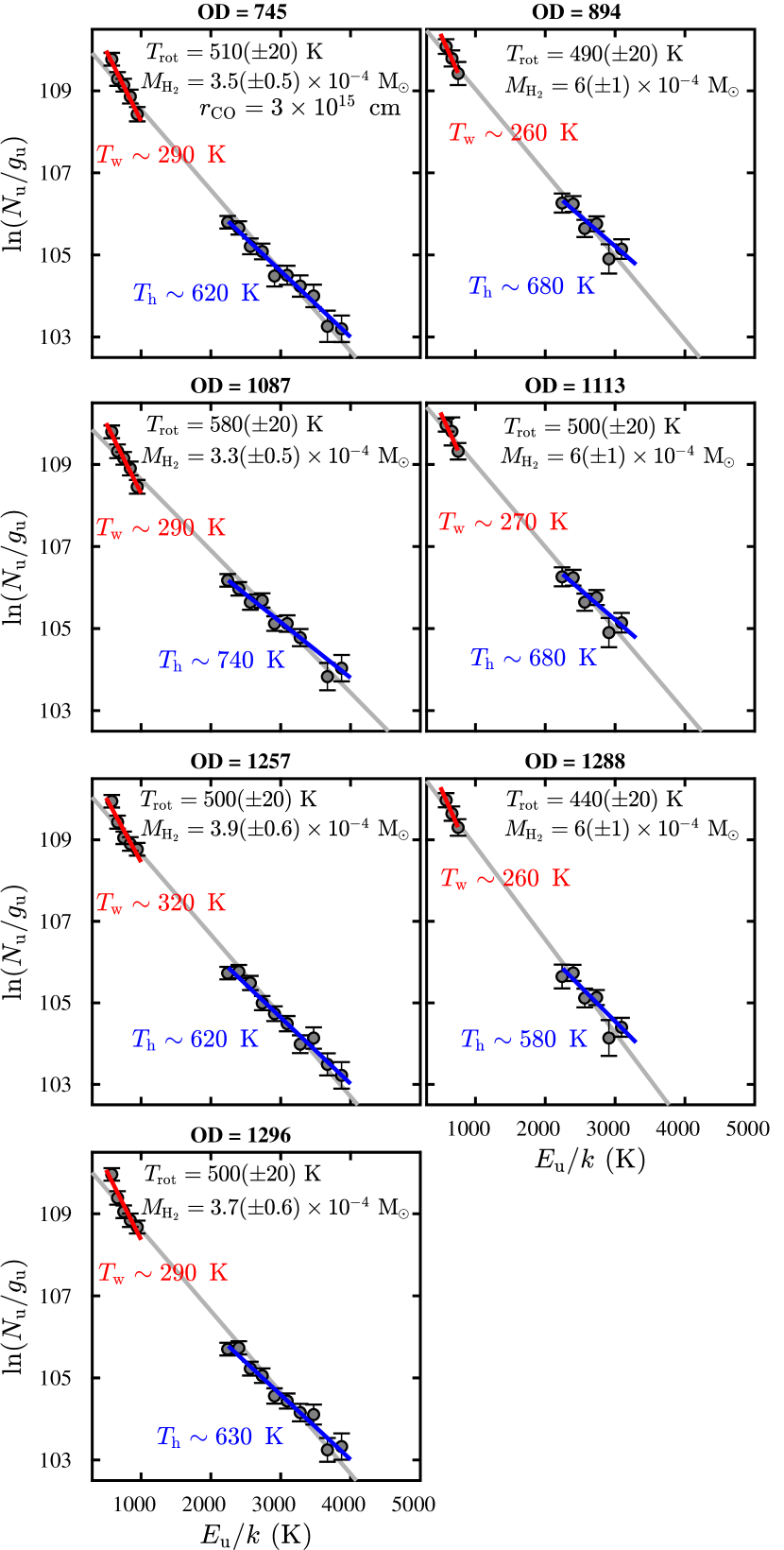
Figure 8: Rotational diagram of the CO molecule in IRC+10216 at different epochs. Analogous to Fig. 6.

Following the same approach of Paper I, we have used the well-known and widely employed rotational diagram (RD) technique (e.g. Goldsmith & Langer 1999) to obtain a first estimate of the (average) excitation temperature ($T_{\rm rot}$) and total mass ($M_{\rm H_{2}}$) of the warm inner layers of the molecular envelopes of our sample. A canonical opacity correction factor, $C_{\tau}$, as defined by Goldsmith & Langer (1999), has been included to take into account moderate optical depth effects (§ A.1). We refer to Paper I for a more detailed description of the method.

4.1 The characteristic size of the CO-emitting layers

To compute the optical depth of the line and to make the corresponding $C_{\tau}$ correction, we need an estimate of the column density of CO, which is computed in a simplified manner dividing the total number of CO molecules ($N_{\rm CO}$) by the projected area of the CO-emitting volume on the sky. The characteristic size of the envelope regions where the CO PACS emission is produced ($r_{\rm CO}$) is one of the main sources of uncertainty since, except for a few targets (see below), these high-$J$ CO-emitting layers are unresolved by PACS. Therefore, the value of $r_{\rm CO}$ needs to be adopted based on several criteria. These criteria are described in much detail in paper I, Appendix B. In the following, we provide a brief summary of the general method and provide additional arguments particularized to the C-rich targets here under study.

For AGB CSEs, a first estimate of the size of the CO-emitting volume can be derived from the envelope temperature structure, $T(r)$, estimated from detailed non-LTE molecular excitation and radiative transfer (nLTEexRT) calculations in the literature. These have been done for many AGB CSEs using low-$J$ CO transitions (typically $J_{\rm u}$$\la$6), and, for a few cases, also using certain CO transitions from higher $J$ levels (see e.g., Decin et al. 2010; Khouri et al. 2014; Danilovich et al. 2014; Maercker et al. 2016; Van de Sande et al. 2018). As deduced from these studies, the gas temperature is approximately 1000-2000 K close to the dust condensation radius ($\sim$5-15 $\rm R_{\star}$), and decreases gradually towards the outermost layers approximately following a power-law of the type $\sim$1/r^α, with $\alpha\sim$0.5-1.0. Such models also exist in literature for three targets in our C-rich sample: IRAS 15194-5115, CIT 6 and IRC+10216 (Ryde et al. 1999; Schöier et al. 2002; De Beck et al. 2012). According to this, the high-excitation transitions observed with PACS require relative proximity to the central star and, in particular, we anticipate that regions with a few hundred kelvin, as deduced from our RDs (Figs. 6 and 8), should not extend much farther than a few $10^{15}$ cm ($\rm\la 10^{2}\,R_{\star}$) in AGB stars.

An additional constraint on the radius can be imposed from the fact that the deepest layer traced by the observed CO emission must be such that $\tau<1$ because of the almost null escape probability from deeper, very optically thick regions (§ A.1). For all our AGB CSEs, we have explored a range of radii around 1$\times 10^{\rm 15}$ cm (Fig. 14). We found that values around $r_{\rm CO}$$\sim$[1-4]$\times 10^{\rm 15}$ cm result in line optical depths close to, but smaller than unity (typically $\tau_{J=14\rightarrow 13}\sim$0.5-0.9) that yield moderate $C_{\tau}$ opacity correction factors for lines with $J_{\rm u}$$<$19 and negligible for higher-$J$ transitions. For $r_{\rm CO}$$<$1$\times 10^{\rm 15}$ cm, the opacity of the CO $J$=14-13 line, which is the optically thickest transition in our sample, becomes larger than 1 in all our targets (also including post-AGBs and yPNes).

We have checked that the range of plausible radii found for the AGB CSEs in our sample, $r_{\rm CO}$$\sim$[1-4]$\times 10^{\rm 15}$ cm, is consistent with the upper limits to the size of their envelopes deduced from the PACS spectral cubes and/or photometric maps by da Silva Santos (2016) and with any other information on the molecular envelope extent from the literature. IRC+10216 is the only AGB CSE that is partially resolved in the PACS cubes, and it is also the closest in our sample. The PACS cubes show a slightly extended source (with a half-intensity size 4$\sigma$ above the instrument PSF in both bands) that implies a deconvolved Gaussian radius of about 2″, that is $\sim 4\times 10^{15}$ cm at $d$=150 pc. This value is in good agreement with the lower limit to $r_{\rm CO}$ needed to satisfy the $\tau_{J=14\rightarrow 13}<$1 criteria in this target, $r_{\rm CO}$$\sim$2$\times 10^{\rm 15}$ cm. In this case, we then rather confidently use an intermediate value of $r_{\rm CO}$=3$\times 10^{\rm 15}$ cm.

Contrary to AGBs, for post-AGBs and yPNe there are no model temperature profiles in the literature of the molecular gas in the CSEs (except for the rotating, circumbinary disk of the Red Rectangle, § 6.1.1).

The range of representative radius adopted for post-AGBs and yPNe is $r_{\rm CO}$=[0.4-4]$\times 10^{\rm 16}$ cm (Table 1) based on a moderate opacity criteria, the extent of the emission in the PACS cubes and photometric maps, and on additional information on the extent of the intermediate-to-outer molecular envelope from the literature. In particular, in AFGL 2688, a deconvolved diameter of $\sim$4″ in the PACS blue band suggests that $r_{\rm CO}$$\la 1\times 10^{16}$ cm (at $d$=340 pc). Previous CO $J$=2-1 mapping observations identified a compact shell of radius $\sim$2″ ($\sim$5$\times 10^{\rm 15}$cm) around the center of the nebula (Cox et al. 2000). Since the CO $J$=14-13 emission is optically thick at $r_{\rm CO}$$\la$6$\times 10^{\rm 15}$ cm (as shown in Fig. 14), we adopt as representative radius an intermediate value of $r_{\rm CO}$=8$\times 10^{\rm 15}$ cm. HD 44179 (The Red Rectangle) is a point-source in the PACS photometric maps, therefore, for a distance of 710 pc, $r_{\rm CO}$ should be of the same order as in AFGL 2688, which is roughly consistent with interferometric observations (e.g., Bujarrabal et al. 2016). For IRAS 16594-4656, only a very loose upper limit to the radius of $r_{\rm CO}$$<$3$\times 10^{\rm 16}$ cm is inferred from optical images and H₂ emission maps in this object (e.g., Hrivnak et al. 2008). We explored the range, $r_{\rm CO}\sim 0.8-2\times 10^{16}$, similar to AFGL 2688, and adopted as a reference value the midpoint value where $\tau_{J=14\rightarrow 13}\sim$0.7.

All yPNe in our sample are point-sources in the PACS spectral cubes, which means that the upper limit to the radius is of about $r_{\rm CO}$$\la$1″$\sim$[1-2]$\times 10^{\rm 16}$ cm for AFGL 618, and $\sim$[4-6]$\times 10^{\rm 16}$ cm for the rest. They are known to have central H ii regions that have recently formed as the star has become progressively hotter along the PNe evolution. Because the CO envelope surrounds the ionized nebula, a lower limit to $r_{\rm CO}$ can be established from the extent of the latter. Taking this into account, we set a representative radius to $r_{\rm CO}$=1$\times 10^{\rm 16}$ cm for AFGL 618 (Sanchez Contreras et al. 2017; Lee et al. 2013), and $r_{\rm CO}$=4$\times 10^{\rm 16}$ cm for the rest (see e.g., Danehkar & Parker 2015; Castro-Carrizo et al. 2010).

Given the uncertainty in $r_{\rm CO}$, we have systematically explored a range of radii around optimal/plausible values of $r_{\rm CO}$ to asses the impact of this parameter in our results (Fig. 14). The opacity correction increases the smaller $r_{\rm CO}$ is, therefore the slope and y-intercept of the RD increase as a direct result of the frequency-dependence of C_τ (§ A.1), which results in lower values of $T_{\rm rot}$ and larger values of $N_{\rm CO}$, thus $M_{\rm H_{2}}$. This also means that, in practice, only the lowest-frequency-points are affected by C_τ, while the highest-frequency transitions (i.e., highest excitation energies) are unaltered regardless of the radius that we chose within the reasonable constraints that we have put.

4.2 Non-LTE effects

In Paper I we examine and discuss extensively the impact of non-LTE excitation effects (if present) on the values of $T_{\rm rot}$ and $M_{\rm H_{2}}$ derived from the RDs in a sample of 26 non C-rich evolved stars with mass-loss rates in the range $\dot{M}$$\sim$2$\times 10^{\rm-7}$-1$\times 10^{\rm-4}$ $\rm M_{\sun}\,yr^{-1}$. The C-rich targets studied here have on average larger mass-loss rates than those in Paper I, therefore, using a similar reasoning, the CO population levels are also most likely close to thermalization in the inner dense regions of the CSEs under study.

This is further supported by nLTEexRT computations of a selection of high-$J$ CO transitions observed with PACS (from $J_{\rm u}$=14 to 38) by Lombaert et al. (2016). Their sample included all our targets except for AFGL 2513 and IRC+10216. These authors conclude that over a broad range of mass-loss rates ($\dot{M}$$\sim$10^-7-2$\times 10^{\rm-5}$ $\rm M_{\sun}\,yr^{-1}$) the CO molecule is predominantly excited through collisions with H₂, with a minor effect of FIR radiative pumping due to the dust radiation field. The role of dust-excitation on FIR CO lines was also investigated by Schöier et al. (2002) and found to be of minor importance for AGBs with typical mass-loss rates of $\sim 10^{-5}\rm\,M_{\sun}\,yr^{-1}$. We assess the FIR pumping effect further in Section 5.3, where we study multi-epoch RDs of IRC+10216, which is a source with well-known CO line variability.

We stress that even under non-LTE conditions, for a simple diatomic molecule like CO, the RD method provides a reliable measure of the total mass within the emitting volume. Although $T_{\rm rot}$ may deviate from the kinetic temperature in regions where the local density is lower than the critical densities of the transitions considered ($n_{\rm crit}$$\sim$5$\times 10^{\rm 5}$-3$\times 10^{\rm 6}$  cm^-3, for $J_{\rm u}$=14 and 27, respectively, and $n_{\rm crit}$$\approx$10⁶-10⁷  cm^-3 for $J_{\rm u}$$>$27), it does describe quite precisely the molecular excitation, i.e.  the real level population. Therefore, the total number of emitting molecules (and, thus, the mass) is quite robustly computed by adding up the populations of all levels. This is also supported by the good agreement (within uncertainties) between the mass-loss rates derived from this (and other works) using similar LTE approximations, and those obtained from nLTEexRT models (including PACS lines for a few targets) – see paper I and Section 6.2.

As discussed in paper I, conceivable LTE deviations would have its largest impact on the excitation temperature of the hot component, since high-$J$ levels have the lowest critical densities (see above). If this is the case, in low mass-loss rate objects, the value of $T_{\rm rot}$ deduced for the hot component could deviate from the temperature of the gas and approach to that of the dust within the CO-emitting volume. We note that, in any case, the gas and dust temperatures, although not equal, are not excessively divergent in the warm envelope regions around $\sim$10¹⁵ cm under study (e.g., Danilovich et al. 2014; Schöier et al. 2002).

5 Results

5.1 Gas temperatures and masses

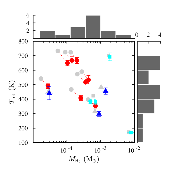
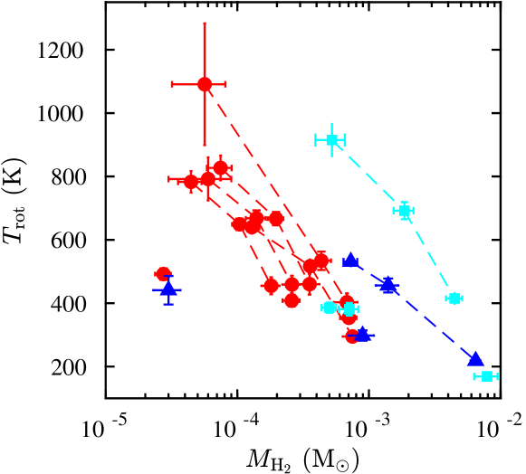
Figure 9: Summary of the RD results. Top: The colored symbols correspond to the opacity corrected values (single fit) which are connected by dotted lines to the corresponding uncorrected values in gray; on the sides we show the histograms of temperature and mass of the single fits; in the case of IRC+10216 we show weighted averages of four observations. Bottom: temperature and mass of the warm and hot components connected by dashed lines for the same target (if applicable).

The opacity-corrected RDs of the CO molecule are plotted in Fig. 6 and in Fig. 8, where multi-epoch RDs for IRC+10216 are separately shown, together with the best-fit parameters using a single-temperature component (gray line) and double-temperature component (red and blue lines). For 8 out of 14 sources, the RDs include CO transitions with upper-level energies that range from $E_{\rm u}$$\sim$580 K to $E_{\rm u}$$\la$2000-3000 K. For 6 targets, CO transitions with upper-level energies of up to $E_{\rm u}$$\sim$5000 K are also detected. Our temperatures for the group of AGBs are consistent with the ones reported in Nicolaes et al. (2018) within the uncertainties, although for many AGBs we find lower values because of the opacity correction term that we have included.

There are cases where it is clear by the analysis of residuals that a single straight line does not fit the entire range of excitation energies. That is the case of V Hya, IRAS 16594-4656, AFGL 3116, CIT 6 and AFGL 618. Because it is not always clear by eye whether the slope changes and at which point it occurs, we used the Bayesian information criterion (BIC) to help us deciding where to split the diagram and to quantify significance. This is explained in the appendix A.2 and illustrated in the supplementary Fig. 16.

We provide the fitting parameters in Table 1 corresponding to a single-fit and a double-component fit in targets where a single line does not equally fit all data points. As in Paper I, we call these two components ”warm” and ”hot” with $T_{\rm w}<T_{\rm single}<T_{\rm h}$. Their mean temperatures are $\overline{T}_{\rm w}\sim$ 400 K and $\overline{T}_{\rm h}\sim$ 820 K respectively. The corresponding masses are $M_{\rm w}$ and $M_{\rm h}$ with the former being 4-10 times larger than the latter. We find single-fit rotational temperatures in the range $T_{\rm rot}$$\sim$ 200-700 K with some of the post-AGBs and yPNe being the targets with the coolest gas, except for the yPNe AFGL 618 which has the largest rotational temperature in our sample similar to that of the warmest AGB CSEs.

The total number of CO molecules is in the range $N_{\rm CO}$$\sim 10^{49}-10^{51}$, resulting in column densities of $N^{\rm col}_{\rm CO}$$\sim 10^{16}-10^{19}$ $\rm cm^{-2}$ for the adopted radii (Table 1). To estimate the total gas mass from CO we assumed the same fractional abundance $X_{\rm CO}=8\times 10^{-4}$ (e.g. Teyssier et al. 2006) with respect to $\rm H_{2}$ for all targets. The single-fit values of the total mass of the CO-emitting volume range between $M_{\rm H_{2}}$$\sim$3$\times$10^-5 $\rm M_{\sun}$ (V Cyg and HD 44179) and $\sim$8$\times$10^-3 $\rm M_{\sun}$ (IRAS 21282+5050), with a median value of $M_{\rm H_{2}}$$\sim$4$\times$10^-4 $\rm M_{\sun}$.

Figure 9 shows the single-fit temperature versus mass for the opacity corrected diagram (colored symbols) and uncorrected (gray symbols). The opacity-correction results in changes in $T_{\rm rot}$ of 10-15% in AGBs, and lower than 5% in post-AGBs and yPNe. In mass this typically corresponds to 60% in AGBs and lower in the post-AGBs and AFGL 618 ($<10$% in $M_{\rm H_{2}}$), and negligible in the other three yPNes. Figure 14 shows that $\tau_{J=14-13}$ is close to unity but it quickly falls off with increasing $J$ meaning that $C_{\tau}\rightarrow 0$ for $E_{\rm u}/k>2000$ K, and that $M_{\rm h}$, in particular, is not underestimated by opacity effects.

As in Paper I, we find an anti-correlation between $M_{\rm H_{2}}$ and $T_{\rm rot}$, especially if we consider only the group of AGBs (Fig. 9). In general, post-AGBs and yPNe have the the highest masses. One clear exception to trend is The Red Rectangle, which is one of the least massive targets (with only a few $\sim$10^-5 $\rm M_{\odot}$ yr^-1) in contrast to the rest of post-AGBs and yPNe. This is not surprising given the nature of this object, which is the prototype of a special class of post-AGB objects with hot rotating disks and tenuous winds very different from the massive and fast (high-momentum) outflows of standard pre-PNe (Bujarrabal et al. 2016, and references therein).

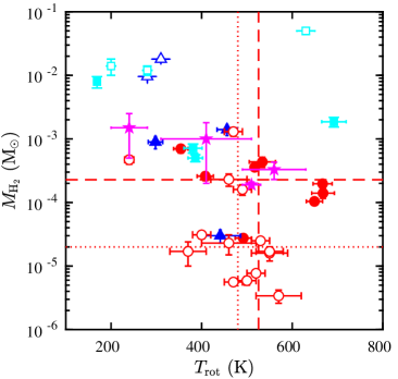
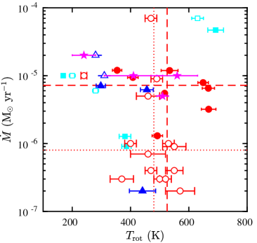
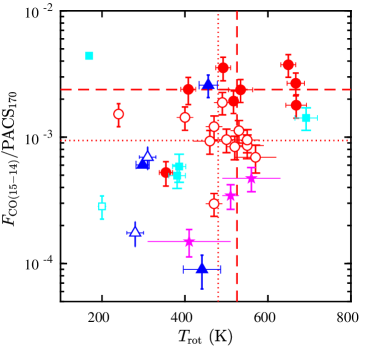
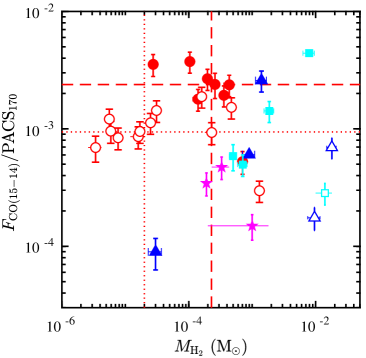
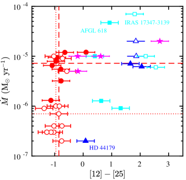
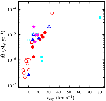
Figure 17: Supplementary plots. Temperature, mass, mass-loss-rate, line to continuum ratio and IRAS color of our sample of C-rich (filled symbols) and O-rich stars in Paper I (open symbols and magenta pentagrams). The color code is the same as in Fig. 1.

We also investigated the correlation between the CO $J=15-14$ flux and the gas mass and find that the strongest CO emitters have tendentially more massive envelopes, although there is a significant scatter (Fig. 17). Also, the targets with the highest temperatures have the highest line-to-continuum (F_CO 15-14/PACS₁₇₀) ratios. IRAS 21282+5050, which has the most massive warm envelope in our sample, defies this trend since it shows relatively strong CO $J=15-14$ emission, although its $T_{\rm rot}$$\sim 170$ K is the lowest in the sample. The Red Rectangle appears isolated in a region of rather weak CO emission in spite of relatively high temperatures ($\sim$400-500 K). We compare these results to Paper I in Section 6.3.

5.2 Mass-loss rates

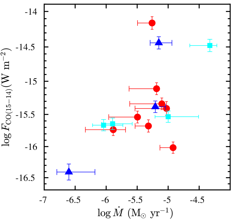
Figure 10: Logarithm of the mass-loss rate versus total CO $J=$15-14 flux.

The mass-loss rates have been estimated by simply dividing the total mass by the crossing time of the CO-emitting layers, that is:

$$\mbox{$\dot{M}$}=\frac{\mbox{$M_{\rm H_{2}}$}\,\mbox{$v_{\rm exp}$}}{\mbox{$r_{\rm CO}$}}$$ (1)

where $v_{\rm exp}$ is the expansion velocity of the gas, which has been taken from literature (Table 4). For the characteristic radius of the CO-emitting region we use the same value ($r_{\rm CO}$) adopted for the opacity correction. We note that this estimate represents a mean or ”equivalent” mass-loss rate assuming constant-velocity spherically-symmetric mass-loss during the time when the warm-inner envelope layers where the CO PACS lines arise were ejected, that is, during the last $\sim$20-50 yr and $\la$300 yr for AGBs and post-AGBs/yPNe, respectively, given the values of $v_{\rm exp}$ and $r_{\rm CO}$.

The mass-loss rates are listed in Table 1. We find a range of values of $\dot{M}\sim 10^{-7}-10^{-5}\rm\leavevmode\nobreak\ M_{\sun}\leavevmode\nobreak\ yr^{-1}$, with a median value in our AGB stars of $\dot{M}$$\sim 6\times 10^{-6}\rm\leavevmode\nobreak\ M_{\sun}\leavevmode\nobreak\ yr^{-1}$. These values are not to be taken as representative of the whole class of C-rich evolved stars, since our sample is small and not unbiased. This is because the objects in the THROES catalogue were originally selected for Herschel observations due to various reasons, probably including their strong CO emission.

As in Paper I, we investigated a possible correlation between $\dot{M}$, and $T_{\rm rot}$, $v_{\rm exp}$. We see little evidence of an anti-correlation between $\dot{M}$ and $T_{\rm rot}$, although the relation is strongly influenced by AFGL 618, which is a strong outlier in this parameter space (Fig. 17). In this, and maybe other objects (mainly post-AGB/yPNe), we expect departures from the simple (constant mass-loss rate, spherically symmetric) model adopted to estimate the ”equivalent” $\dot{M}$. We compare the results obtained here and in Paper I in Section 6.3.

Figure 10 shows the logarithm of the integrated flux of the CO $J=15-14$ line versus the logarithm of the mass-loss rate of the single component fit. The upper and lower limit of the errorbars in $\dot{M}$ correspond to a range of radii around the representative one (see Fig. 14). We find a positive trend which is consistent with a power-law relation similar to that found by Lombaert et al. (2016) in their sample of C-rich AGB CSEs with H₂O FIR emission lines.

Separate values of $\dot{M}$ for the hot and warm components are computed for completeness, but the difference found ($M_{\rm h}<M_{\rm w}$) should not be overinterpreted as a recent decrease of the mass-loss rate. The hot and warm components most likely trace adjacent layers of the inner-winds of our targets, with the hot component presumably best sampling regions closer to the center. However, for simplicity and since we ignore the true CO excitation structure, we use the same radius to formally compute $\dot{M}$ for both components. We note that due to the $1/r_{\rm CO}$ dependence, the values of $M_{\rm h}$ and $M_{\rm w}$ can be brought closer to the single-fit value if the warm and hot correspond to different $r_{\rm CO}$. We refrain from discussing $M_{\rm h}$ and $M_{\rm w}$ separately since a more sophisticated analysis, including nLTEexRT modeling, is needed in order to assess mass-loss time variability. For this reason we only compare our single-component mass-loss rates to the literature (§ 6.2).

5.3 The influence of line variability on $T_{\rm rot}$ and $M_{\rm H_{2}}$

We have shown in Fig. 4 the temporal variability of the continuum and line fluxes in the case of the Mira-type variable AGB star IRC+10216. The higher-$J$ CO lines ($E_{\rm u}$$>$2000 K) are the ones that show the strongest variations with time. Here, we are interested in studying how CO line variability affects the values of $M_{\rm H_{2}}$ and $T_{\rm rot}$ derived using the RD method but using data acquired at different epochs. We use the same seven available OBSIDS of IRC+10216 as Teyssier et al. (2015), which span a time period of 551 days (Table 3).

The RDs of IRC+10216 for these seven different observing epochs are shown in Fig. 8, and the results of the RD analysis are tabulated in Table 1, together with the remaining targets. Since three of the OBSIDs corresponding to the ODs 894, 1133 and 1288 have a more restricted wavelength coverage, the fits to the RDs have an inherently larger uncertainty because the fit is more sensitive to the low number statistics. The error-weighted mean (single-fit) rotational temperature and mass are $T_{\rm rot}$$\sim$520 K and $M_{\rm H_{2}}$$\sim$4$\times 10^{-4}$ $\rm M_{\sun}$, respectively.

In Fig. 11, we plot the temperature and the mass, for single- and double-temperature components, versus the operational day of the observations. The bottom panel shows that the total gas mass deduced from the single-fit of the RD or for the warm and hot components does not reflect the line flux variability since it stays essentially constant with time about the average value (dotted lines), well within the estimated uncertainties.

In a similar manner, the temperature of the warm component does not clearly reflect the CO line flux variations, since all multi-epoch values are in good agreement within uncertainties. The hot component is the one that shows the largest variations (perhaps periodic) of the temperature, with $T_{\rm h}$ going $\sim$100 K ($\sim$16%) above the average ($\sim$ 640 K) at OD 1087, and then relaxing back to normal values in the remaining epochs. This variation is echoed in the single-fit value of $T_{\rm rot}$  ($\sim$12%).

Temperature variations are not necessarily expected to be periodic, but if we assume that to be true by fitting a sinusoidal function with the known pulsation period $P=630$ days to the RD parameters, we find that such model accommodates reasonably well the data points corresponding to $T_{\rm h}$ (and also the single-fit $T_{\rm rot}$). It is also possible that IRC+10216 underwent an abrupt change of the physical conditions in its inner wind layers at epoch OD 1087, since the remaining data points by themselves will not justify/indicate periodic variability.

In summary, probably due to a compensation between the changes in the y-intercept and the slope of the RD due to CO line flux variations, which are largest for transitions with the highest $J$, the total gas mass $M_{\rm H_{2}}$ appears to be quite robust to FIR pumping (non-LTE) effects. These, however, could have a measurable, yet moderate impact on the rotational temperatures.

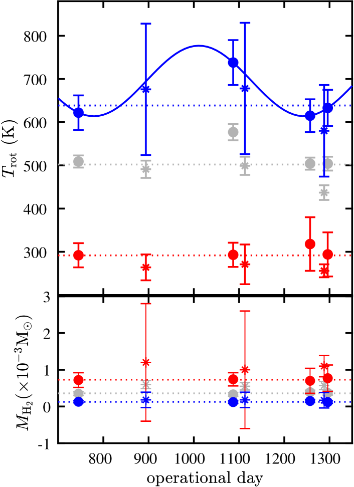
Figure 11: Rotational temperature and mass versus operational day in IRC+10216. Top: sinusoidal fit to the $T_{\rm rot}$variation with fixed period of 630 days (solid line). Bottom: total gas mass over time. In each panel, the dotted lines are the average of each component and the asterisks mark unused data points in the fit (see text). The color code is the same as in Fig. 8.

6 Discussion

6.1 Gas temperatures

The detection of high-$J$ CO rotational lines is an indication of a significant amount of molecular gas under relatively high temperature conditions. From our simple RD analysis we inferred that the average gas temperatures of the layers sampled by FIR CO lines are much larger ($T_{\rm rot}\sim 200-900$ K) than those typically derived from mm/sub-mm observations, which are sensitive to $\la$ 100 K gas from the intermediate-to-outer layers of the envelopes of evolved stars (at $\approx$10¹⁶-10¹⁷ cm, see e.g. De Beck et al. 2010; Schöier et al. 2011).

In a number of targets we identified a double-temperature (”warm” and ”hot”) component. Deviations from a single straight line fit to the RD have been found also in some of the O-rich objects in Paper I and in other previous works using, for example, ISO and/or Herschel/SPIRE CO spectra in a number of AGB and post-AGB CSEs (e.g., Justtanont et al. 2000; Wesson et al. 2010; Matsuura et al. 2014; Cernicharo et al. 2015b; Cordiner et al. 2016). AFGL 618 and IRAS 16594-4656 are the targets whose RDs show the most obvious departure from linearity. IRAS 16594-4656 is particularly interesting since we found a much cooler warm-component of just $T_{\rm w}\sim 220$ K, and a breakpoint at lower energies ($E_{\rm u}/k\approx 1049.9$ K) compared to other targets typically with $T_{\rm w}\sim 450$ K up to $E_{\rm u}/k\approx 1794.3$ K.

As in Paper I, in order to investigate if the double-temperature component is consistent with resulting from the temperature stratification within the inner layers of the CSEs, we compared the hot-to-warm $M_{\rm H_{2}}$ and $T_{\rm rot}$ ratios (Fig. 12), and find that they are correlated. If the temperature profiles in the envelope follow a power-law of the type $T(r)\propto r^{-\alpha}$, with $\alpha$ being a constant, then the trend in Fig. 12 should also follow approximately a power-law function. We find $\alpha\sim 0.4$, which is similar to the value found for the O-rich targets studied in Paper I. The value of $\alpha$ is in agreement with past works that suggested that the kinetic temperature distribution is shallower, with values of $\alpha$ down to $\sim$0.4-0.5, for the inner ($\sim$5$\times 10^{\rm 14}$-3$\times 10^{\rm 15}$ cm) CSE layers De Beck et al. (2012); Lombaert et al. (2016); Matsuura et al. (2014) than for the outer regions, where the steepest temperature variations ($\alpha\sim$1-1.2) are found ($\ga$10¹⁶ cm; Teyssier et al. 2006).

In addition to the average power-law exponent obtained by fitting all the targets simultaneously, we can also derive a value for each individual case applying:

$$\alpha=-\frac{\log(T_{\rm h}/T_{\rm w})}{\log(M_{\rm h}/M_{\rm w})}$$ (2)

as shown in the bottom panel of Fig. 12. In the case of IRC+10216, we find $\alpha=0.45\pm 0.06$ which is in good agreement with the power-law exponent in the inner CSE between 9 and 65 stellar radii (i.e., up to $\sim 3\times 10^{15}\rm\,cm$) deduced from detailed non-LTE excitation and radiative transfer models (De Beck et al. 2012).

Therefore, the empirical relation found between the hot-to-warm ratio of $M_{\rm H_{2}}$ and $T_{\rm rot}$ is consistent with the double-$T_{\rm rot}$ component in some of our targets stemming (at least partially) from the temperature stratification across the inner envelope layers. The two components in the RD do not necessarily imply two distinct/detached shells of gas at different temperatures, but they most likely reflect the temperature decay laws. As explained in Paper I, in case of LTE deviations (not impossible in the lowest mass-loss rate objects), the value of $\alpha$ obtained from this simple approach would more closely represent the dust (rather than the gas) temperature distribution. This needs confirmation by detailed nLTEexRT models to the individual targets, which will be done in a future publication.

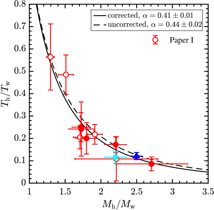
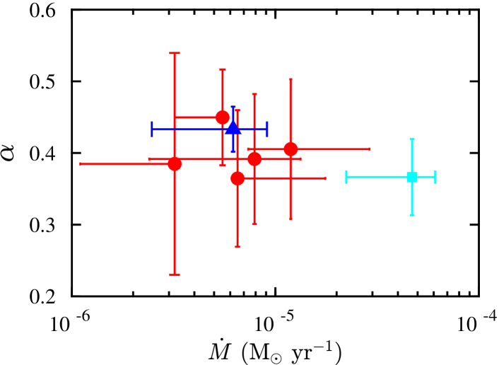
Figure 12: Hot/warm temperature ratio versus hot/warm mass ratio for AGBs and post-AGBs and the power-law index. Top: the lines correspond to power-law fits with index $\alpha=0.4$ for the opacity corrected RDs (solid) and $\alpha=0.44$ for the uncorrected RDs (dashed); the open symbols correspond to the O-rich AGB stars in Paper I. Bottom: power law index for each individual target versus mass-loss rate (single fit).

6.1.1 Individual targets: comparison with previous works

It is not possible to directly compare most of our results with literature because past studies have been focusing on the cold, outer components of CSEs. Prior to Herschel there was a study based on ISO LWS data in roughly the same wavelength range by Justtanont et al. (2000) who also performed RD analysis (without opacity correction). They found $T_{\rm rot}\sim 700(\pm 90)$ K and $T_{\rm rot}\sim 380(\pm 30)$ K for AFGL 618 and AFGL 2688 respectively. We obtained similar results without opacity correction, but introducing this effect lowered these values to $T_{\rm rot}\sim 690(\pm 30)$ K and $T_{\rm rot}\sim 300(\pm 20)$ K. In AFGL 618 the central star is hot enough ($T_{\rm eff}\sim 33000$ K) to produce FUV photons that heat the gas. In AGFL 2688 this is probably not the case since the central star is much cooler ($T_{\rm eff}\sim 7250$ K), so low-velocity shocks are the most likely heating mechanism.

Also partially based on ISO data, Ryde et al. (1999) used a number of spectral lines of CO between $J=1-0$ and $J=21-20$ to infer the kinetic temperature profile across the CSE of IRAS 15194-5115. According to their model, $T_{\rm kin}\sim 400$ K at $r_{\rm CO}\sim$ (1-2)$\times 10^{15}\rm\,cm$, which is in excellent agreement with our opacity-corrected single component $T_{\rm rot}\sim 410$ K for $r_{\rm CO}=2\times 10^{15}\rm\,cm$. This is because, as already pointed out by Ryde et al. (1999), these high-$J$ levels are mainly populated by collisions, therefore they are proxies for the kinetic temperature, at least out to a few $\sim 10^{15}$ cm. Also using ISO data, Schöier et al. (2002) presented a kinetic temperature model for CIT 6 that shows that $T_{\rm kin}\sim 400-500$ K at approximately $r_{\rm CO}\sim$ (1-2)$\times 10^{15}\rm\,cm$, which is consistent with the warm component ($T_{\rm w}\sim 460$ K) that we infer and the representative radius $r_{\rm CO}=2\times 10^{15}\rm\,cm$ adopted. The hot component ($T_{\rm w}\sim 830$ K) found by us would imply that regions closer to the star have an important contribution to the emission of the highest-$J$ lines.

The only star whose inner/warmer (gaseous) CSE had been studied in detail before using Herschel/PACS data is IRC+10216. This was done by Decin et al. (2010) using high-$J$ CO spectral lines to infer the kinetic temperature profile as a function of radial distance. They find $T_{\rm kin}\sim 500-600$ K at $r_{\rm CO}\sim$ (1-2)$\times 10^{15}\rm\,cm$. Here we applied the opacity correction for $r_{\rm CO}=3\times 10^{15}$ cm which seems to be the layer at which $T_{\rm kin}\sim 300$ K in their model. This is also the average value of $T_{\rm w}$ that we found by fitting only the lowest $J$ transitions, wich does not change appreciably with time despite strong line flux variability (Fig. 11). The hot component ($\sim$600-700 K) may correspond to $r_{\rm CO}\sim 1\times 10^{15}\rm\,cm$ according to their model.

Using Herschel/SPIRE data, Wesson et al. (2010) also performed RD analysis of CO spectra and derived $T_{\rm rot}\sim$70-230 K and $T_{\rm rot}\sim$100-200 K for AFGL 618 and AFGL 2688, respectively. The rotational temperatures we find are thus higher than the ones obtained in Wesson et al. (2010) as expected. Further Large-velocity gradient (LVG) calculations by those authors suggested that hot material at approximately $1000$ K might exist at the high-velocity wind region of AFGL 618, which could be the one traced by PACS since we found $T_{\rm h}\sim 900$ K.

For HD 44179 (the Red Rectangle) we obtained $T_{\rm rot}\sim 440$ K, which is about 2-3 times larger than the range of values inferred by Bujarrabal & Alcolea (2013) from Herschel/HIFI lower-$J$ CO observations. It is not surprising that we find a larger value since the higher $J$ lines probed by PACS are probably formed deeper inside the rotating circum-binary disk at the core of this object. Meanwhile follow up analysis has shown more clearly an outflow with $\sim 500$ K (Bujarrabal et al. 2016), but also seems that such temperature conditions could exist in a region of the inner disk with a radius of about $r_{\rm CO}\sim 2\times 10^{15}$ cm, unresolved by PACS. The opacity correction would still be moderate for this value ($\tau_{J=14-13}\sim 0.67$), and it lowers the rotational temperature to $T_{\rm rot}\approx 410$ K which is still within the uncertainties. For the remaining yPNes (IRAS 21282+5050, CPD-568032, Hen 2-113) there are no kinetic temperature models in the literature that we could compare our results to.

6.2 Mass-loss rate

As in Paper I, we have compared the values of the mass-loss rates derived from our simple RD analysis with other values found in the literature mostly from low-$J$ observations, paying special attention to a few targets with detailed non-LTE excitation and radiative transfer analysis of CO data including at least some high-$J$ transitions observed with Herschel. This is also a way of ascertaining the robustness of the RD method.

Figure 13 shows our estimate of the mass-loss rate versus that found in the literature (see Table 4). For each target the markers correspond to the single temperature component for the radius mentioned in Table 1, and the error bars represent the uncertainty in the radius for the adopted $v_{\rm exp}$. We show the computed opacities for the considered radii in each target in the supplementary Fig. 14. The range of values found in literature are shown by the gray shaded area whose bounds are set by the maximum and minimum $\dot{M}$ plus uncertainties when reported (factor of $\sim$3 in AGBs, Ramstedt et al. 2008; De Beck et al. 2010). Those values have been rescaled to the same distance, $v_{\rm exp}$ and $X_{\rm CO}$ here adopted.

Similarly to the non C-rich THROES targets in Paper I, our mass-loss rates are in good agreement with values in the literature within the large uncertainties. In our case, these are dominated by the uncertainty in $r_{\rm CO}$. We see that the range of radii we explored yields a $\dot{M}$ that fits within the shaded area. In many cases, the error bars are truncated at the upper limit above which the line opacities would be too large to allow reliable estimates of the masses and mass-loss rates (see Fig. 14). For example, in the case of AFGL 3068 this seems to imply smaller radius than what we have adopted to better match the values in literature.

In the case of IRC+10216, the opacity correction for $r_{\rm CO}=2\times 10^{15}$ cm (instead of $r_{\rm CO}$=3$\times 10^{\rm 15}$ cm) would result in a mass-loss of $\dot{M}\approx 1.4\times 10^{-5}\leavevmode\nobreak\ \rm M_{\sun}\leavevmode\nobreak\ yr^{-1}$ (not displayed) that would best match the estimate from mm observations. However in these circumstances the expected opacities in the lowest $J$ lines would be too large ($\tau\gg 1$). Nonetheless, the derived $T_{\rm w}$ and $T_{\rm h}$ are consistent with kinetic temperature profile models as explained in Section 6.1. We find an average value of four OBSIDs of $\dot{M}\sim 5\times 10^{-6}\leavevmode\nobreak\ \rm M_{\sun}\leavevmode\nobreak\ yr^{-1}$, which is lower than the range $\dot{M}\sim$(1-3)$\times 10^{-5}\leavevmode\nobreak\ \rm M_{\sun}\leavevmode\nobreak\ yr^{-1}$ scaled from Teyssier et al. (2006); De Beck et al. (2010, 2012); Guélin et al. (2017). However the value obtained for the warm component agrees with the lower limit of this range (because of the larger $M_{\rm H_{2}}$). We obtain $T_{\rm w}\sim 300$ K and $\dot{M_{\rm w}}\sim$1$\times 10^{-5}\leavevmode\nobreak\ \rm M_{\sun}\leavevmode\nobreak\ yr^{-1}$ for a radius of $r_{\rm CO}=3\times 10^{15}$ cm, in good agreement with the results of radiative transfer modeling of the same high $J$ CO lines by Decin et al. (2010). Scaling their $\dot{M}$ to the same $d$ and $X_{\rm CO}$ gives $\dot{M}\sim$1.2$\times 10^{-5}$ $\rm M_{\odot}$ yr^-1 with an uncertainty of a factor 2.

For V Hya we obtained $\dot{M}\sim 8\times 10^{-6}\leavevmode\nobreak\ \rm M_{\sun}\leavevmode\nobreak\ yr^{-1}$ which is lower than $\dot{M}\sim 3\times 10^{-5}\leavevmode\nobreak\ \rm M_{\sun}\leavevmode\nobreak\ yr^{-1}$ from Camps (2011) who performed radiative transfer calculations using the same PACS spectrum. In this case, however, the spatio-kinematic structure of the molecular outflow is more complex than assumed here. In particular, multiple kinematic (fast and slow) components seem to be present Hirano et al. (2004); Sahai et al. (2009), which not only translates into a larger uncertainty in the characteristic value of $v_{\rm exp}$ in the PACS CO-emitting layers, but also implies that the ”equivalent” mass-loss rate is particularly questionable.

As for V Hya, for pPNe and yPNe, the assumption of constant-velocity spherically- symmetric mass loss may also not hold. For completeness, the mass-loss rates estimates for these targets are shown Table 4, but they are subject to larger uncertainties and have to be interpreted with caution. We have checked that, even in these cases, our values are in good agreement with previous estimates (making similar simplifying assumptions) in the literature. For example, for the Red Rectangle, we obtained $\dot{M}\sim 2\times 10^{-7}$ $\rm M_{\odot}$ yr^-1 which is within the (scaled) range of $\dot{M}\sim$(0.2-1.4)$\times 10^{-7}$ $\rm M_{\odot}$ yr^-1 reported by De Beck et al. (2010).

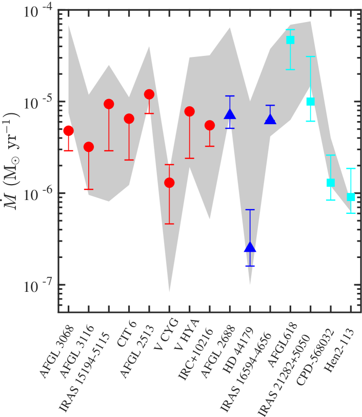
Figure 13: Comparison between the mass-loss rate in this work and the literature. The markers correspond to the representative radii listed in Table 1 for each target and the error bars are mass-loss rates for a given range of radii. The shaded area encloses the range of values found in literature scaled to the same parameters here assumed (see text).

In summary, our results are consistent with the literature within the typical uncertainties, but it is hard to tell what is the exact cause of the slight discrepancies from case to case. One obvious reason is that the simple RD method and our assumption of a characteristic value of $r_{\rm CO}$ (unknown, but crudely constrained from first principles and observations) only provides a rough estimate of the mass-loss. We also note, that the bulk of the CO emission under study is produced in the warm inner layers of the CSEs of our targets down to a location where $\tau$$\sim$1. For very optically thick CSEs, there may be an additional amount of gas that is not fully recovered after the moderate opacity correction applied. Another reason for $\dot{M}$ discrepancies is the different number of transitions and range of $E_{\rm u}$ covered by different studies. Non-LTE excitation and radiative transfer models of the CO emission including a wide range of $J$- transitions is needed to obtain accurate estimates of the mass-loss rates and, in particular, to address $\dot{M}$ time modulations.

6.3 Comparison between the sample of O-rich and C-rich stars

In the Appendix we provide Fig. 17 where we plot together the results presented here to the ones obtained for the sample of O-rich and S-type stars in Paper I.

We find that the range of $T_{\rm rot}$ is approximately the same among C-rich and O-rich stars, but the O-rich AGBs have less massive CSEs by typically one order of magnitude, and lower expansion velocities. This in turn reflects on lower mass-loss rates on average. The scenario is reversed in the groups of PNes with the few O-rich PNes having more warm gas than the carbon counterparts. Probably the O-rich AGB stars studied in Paper I are typically low massive stars with very large evolution times, while the O-rich post-AGBs and PNe are very massive objects that have undergone through the Hot Bottom Burning stage.

We stress that despite these trends being indicative of clear differences in the properties of the CSEs of the targets in the THROES catalogue, they may not be a general property of C-rich versus non C-rich targets, since our samples are not necessarily unbiased and they are definitely not statistically significant.

7 Summary

In this paper (Paper II), we use Herschel/PACS FIR spectra of a sample of 15 C-rich evolved stars, including AGBs, post-AGBs and yPNe, from the THROES catalogue (Ramos-Medina et al. 2018b). These data contain valuable information about the physical-chemical properties of evolved stars as shown, for instance, by the striking differences of spectral features (molecular, atomic/ionized and solid state) as a function of evolutionary stage. In this work, we focus on the rotational spectrum of CO (up to $J=45-44$) which was used as a proxy for the molecular component of the gas in the warm regions of the CSEs. Our findings can be summarized as follows:

• Due to Herschel’s higher sensitivity compared to ISO, the range of detected ¹²CO  transitions has been extended to high rotational levels of up to $J_{\rm u}$=45 in low-to-intermediate mass evolved stars. Rotational diagrams using high-excitation CO ($v$=0) rotational emission lines, with upper-level energies $E_{\rm u}$$\sim$580 to 5000 K, have been plotted to estimate rotational temperatures ($T_{\rm rot}$), total molecular mass in the CO-emitting layers ($M_{\rm H_{2}}$) and average mass-loss rates during the ejection of these layers ($\dot{M}$).

• The range of temperatures found in our sample, $T_{\rm rot}$$\sim$200-700 K, is larger than what had been deduced from mm/sub-mm observations, and even Herschel/HIFI and SPIRE observations, confirming that PACS CO lines probe deeper layers yet poorly studied to date (typically, $\approx$10¹⁵ cm for AGBs and $\approx$10¹⁶ cm for post-AGBs and yPNes).)

• The total gas mass of the warm envelope layers sampled by PACS data are between $M\sim 10^{-5}-10^{-3}\leavevmode\nobreak\ \rm M_{\sun}$, with post-AGBs and yPNe being overall more massive.

• We find clearly different temperature distributions for the different classes with AGBs having typically hotter gas (up to $T_{\rm rot}\sim 1000$ K) than post-AGBs ($T_{\rm rot}\la 500$ K) and yPNes ($T_{\rm rot}\la 400$ K). The yPN AFGL 618 is a clear outlier with a very high amount ($M_{\rm H_{2}}$$\sim$2$\times 10^{\rm-3}$ $\rm M_{\sun}$) of rather hot (up to T_h$\sim$900 K) gas, similar to the most massive AGBs in the sample.

• For AFGL 3116, CIT 6, AFGL 2513, V Hya, IRAS 16594-4656 and AFGL 618 a double temperature (hot and warm) component is inferred from the RDs. The mean temperatures of the warm and hot components are $\sim$400 K and $\sim$820 K, respectively. The mass of the warm component ($\sim$10^-5-8$\times$10^-3$\rm M_{\sun}$) is always larger than that of the hot component, by a factor $\sim$4-10.

• The warm-to-hot $M_{\rm H_{2}}$ and $T_{\rm rot}$ ratios in our sample are correlated and are consistent with an average temperature radial profile of $T\propto$ $r^{-0.4}$, that is, slightly shallower than in the outer envelope layers, in agreement with recent studies.

• The mass-loss rates estimated are in the range $\dot{M}$$\approx$10^-7-10^-4$\rm M_{\odot}$ yr^-1, in agreement (within the uncertainties) with values found in the literature for our targets.

• We investigated the impact of CO line flux variability on the values of $M_{\rm H_{2}}$ and $T_{\rm rot}$ derived from the simple RD analysis. We studied in detail the case of the Mira-variable AGB star IRC+10216, for which multi-epoch PACS data exist. In spite of strong line flux variability we find that the total gas mass and the average temperature derived from the RDs at different epochs are minimally affected. Only the hot component does show the sign of line variability ($\delta T/T\sim 16$%), roughly in-phase with the continuum periodicity.

• Similarly to Paper I, we find an anti-correlation between $T_{\rm rot}$ and $M_{\rm H_{2}}$, which may result from a combination of CO line cooling and opacity effects, and we find a correlation between $\dot{M}$ and $v_{\rm exp}$, which is consistent with the wind acceleration mechanism being more efficient the more luminous/massive the star is. These trends had been reported in previous studies using low-$J$ CO transitions.

We show that high-$J$ CO emission lines probed by Herschel/PACS are good tracers of the warm gas ($T\sim 200-900$ K) surrounding evolved carbon stars. Using the simple RD technique, we have provided systematic and homogeneous insight into the deepest layers of these CSEs, though it relies on several approximations. Detailed non-LTE excitation and radiative transfer calculations are needed to determine the temperature stratification of the CSEs, to infer mass-loss rates and to address their time-variability.

Table 1: Results of the CO rotational diagram analysis with opacity correction and double-component fit. The assumed distance ($d$), expansion velocity ($v_{\rm exp}$) and radius ($r_{\rm CO}$), the derived rotational temperature ($T_{\rm rot}$), CO column density ($N^{\rm col}_{\rm CO}$), total mass of $\rm H_{2}$ within the CO emitting-volume ($M_{\rm H_{2}}$), mass-loss rate ($\rm\dot{M}=\mbox{$M_{\rm H_{2}}$}\times v_{\rm exp}/r_{\rm CO}$) and ratio between opacity corrected and uncorrected total masses.

Target	$d$ (pc)	$v_{\rm exp}$ $\rm(km\leavevmode\nobreak\ s^{-1})$	$r_{\rm CO}$ (cm)	$T_{\rm rot}$(K)	$N^{\rm col}_{\rm CO}$$\rm(cm^{-2})$	$M_{\rm H_{2}}$$\rm(\rm M_{\sun})$	$\dot{M}$ $\rm(\rm M_{\sun}\leavevmode\nobreak\ yr^{-1})$	Correction $M_{\rm H_{2}}$
AFGL 3068	1100	13	$6\times 10^{15}$	350$\pm$20	$3\times 10^{18}$	$7(\pm 1)\times 10^{-4}$	$5\times 10^{-6}$	1.6
AFGL 3116	630	14	$2\times 10^{15}$	670$\pm$30	$5.4\times 10^{18}$	$1.4(\pm 0.2)\times 10^{-4}$	$3\times 10^{-6}$	1.6
				460$\pm$30	$9.8\times 10^{18}$	$2.6(\pm 0.4)\times 10^{-4}$	$6\times 10^{-6}$	1.8
				790$\pm$70	$2.4\times 10^{18}$	$6(\pm 3)\times 10^{-5}$	$1\times 10^{-6}$	1.3
IRAS 15194-5115	500	23	$2\times 10^{15}$	410$\pm$20	$9.8\times 10^{18}$	$2.6(\pm 0.4)\times 10^{-4}$	$9\times 10^{-6}$	1.9
CIT 6	440	21	$2\times 10^{15}$	670$\pm$20	$7.4\times 10^{18}$	$2(\pm 0.3)\times 10^{-4}$	$7\times 10^{-6}$	1.6
				460$\pm$30	$1.3\times 10^{19}$	$3.5(\pm 0.7)\times 10^{-4}$	$1\times 10^{-5}$	1.7
				830$\pm$40	$2.8\times 10^{18}$	$7(\pm 2)\times 10^{-5}$	$2\times 10^{-6}$	1.3
AFGL 2513	1760	26	$3\times 10^{15}$	530$\pm$30	$7.3\times 10^{18}$	$4.4(\pm 0.8)\times 10^{-4}$	$1\times 10^{-5}$	1.6
				400$\pm$30	$1.1\times 10^{19}$	$7(\pm 1)\times 10^{-4}$	$2\times 10^{-5}$	1.7
				1100$\pm$200	$9.5\times 10^{17}$	$6(\pm 2)\times 10^{-5}$	$2\times 10^{-6}$	1.3
V Cyg	271	15	$1\times 10^{15}$	490$\pm$20	$4.2\times 10^{18}$	$2.7(\pm 0.4)\times 10^{-5}$	$1\times 10^{-6}$	1.6
V Hya	380	24	$1\times 10^{15}$	650$\pm$20	$1.6\times 10^{19}$	$1.0(\pm 0.1)\times 10^{-4}$	$8\times 10^{-6}$	1.9
				460$\pm$30	$2.7\times 10^{19}$	$1.8(\pm 0.3)\times 10^{-4}$	$1\times 10^{-5}$	2.1
				780$\pm$40	$6.7\times 10^{18}$	$4.5(\pm 0.9)\times 10^{-5}$	$3\times 10^{-6}$	1.4
AFGL 2688	340	20	$8\times 10^{15}$	300$\pm$20	$2\times 10^{18}$	$9(\pm 2)\times 10^{-4}$	$7\times 10^{-6}$	1.2
HD 44179	710	10	$4\times 10^{15}$	440$\pm$50	$3\times 10^{17}$	$3.2(\pm 0.8)\times 10^{-5}$	$2\times 10^{-7}$	1.1
IRAS 16594-4656	1800	14	$1\times 10^{16}$	460$\pm$20	$2\times 10^{18}$	$1.4(\pm 0.3)\times 10^{-3}$	$6\times 10^{-6}$	1.4
				220$\pm$5	$1\times 10^{19}$	$6.5(\pm 0.6)\times 10^{-3}$	$3\times 10^{-5}$	1.5
				530$\pm$20	$1\times 10^{18}$	$7.3(\pm 0.9)\times 10^{-4}$	$3\times 10^{-6}$	1.3
AFGL 618	900	80	690$\pm$30	$1\times 10^{16}$	$2.8\times 10^{18}$	$1.9(\pm 0.3)\times 10^{-3}$	$5\times 10^{-5}$	1.1
				415$\pm$20	$6.8\times 10^{18}$	$4.5(\pm 0.6)\times 10^{-3}$	$1\times 10^{-4}$	1.1
				915$\pm$60	$7.9\times 10^{17}$	$5(\pm 1)\times 10^{-4}$	$1\times 10^{-5}$	1
IRAS 21282+5050	2000	14	$4\times 10^{16}$	170$\pm$10	$7.5\times 10^{17}$	$8(\pm 2)\times 10^{-3}$	$1\times 10^{-5}$	1.2
CPD-568032	1530	22.6	$4\times 10^{16}$	380$\pm$20	$6.8\times 10^{16}$	$7(\pm 1)\times 10^{-4}$	$1\times 10^{-6}$	1
Hen 2-113	1230	23	$4\times 10^{16}$	390$\pm$20	$4.7\times 10^{16}$	$5.0(\pm 0.6)\times 10^{-4}$	$9\times 10^{-7}$	1

Table 2: Continued.

Target	$d$ (pc)	$v_{\rm exp}$ $\rm(km\leavevmode\nobreak\ s^{-1})$	$r_{\rm CO}$ (cm)	$T_{\rm rot}$(K)	$N^{\rm col}_{\rm CO}$$\rm(cm^{-2})$	$M_{\rm H_{2}}$$\rm(\rm M_{\sun})$	$\dot{M}$ $\rm(\rm M_{\sun}\leavevmode\nobreak\ yr^{-1})$	Correction $M_{\rm H_{2}}$
IRC+10216
(OD 745)	150	14.5	$3\times 10^{15}$	510$\pm$20	$5.8\times 10^{18}$	$3.5(\pm 0.5)\times 10^{-4}$	$5\times 10^{-6}$	1.8
				290$\pm$30	$1.2\times 10^{19}$	$7(\pm 2)\times 10^{-4}$	$1\times 10^{-5}$	1.9
				620$\pm$40	$2.3\times 10^{18}$	$1.3(\pm 0.3)\times 10^{-4}$	$2\times 10^{-6}$	1.3
(OD 894)*	150	14.5	$3\times 10^{15}$	490$\pm$20	$1\times 10^{19}$	$6(\pm 1)\times 10^{-4}$	$9\times 10^{-6}$	2.2
				260$\pm$30	$2\times 10^{19}$	$1(\pm 1)\times 10^{-3}$	$2\times 10^{-5}$	2.1
				680$\pm$150	$3\times 10^{18}$	$2(\pm 2)\times 10^{-4}$	$3\times 10^{-6}$	1.5
(OD 1087)	150	14.5	$3\times 10^{15}$	580$\pm$20	$5.5\times 10^{18}$	$3.3(\pm 0.5)\times 10^{-4}$	$5\times 10^{-6}$	1.7
				290$\pm$30	$1.2\times 10^{19}$	$7(\pm 2)\times 10^{-4}$	$1\times 10^{-5}$	1.7
				740$\pm$50	$2.1\times 10^{18}$	$1.2(\pm 0.4)\times 10^{-4}$	$2\times 10^{-6}$	1.3
(OD 1113)*	150	14.5	$3\times 10^{15}$	500$\pm$20	$9\times 10^{18}$	$6(\pm 1)\times 10^{-4}$	$8\times 10^{-6}$	2.1
				270$\pm$50	$1.7\times 10^{19}$	$1(\pm 3)\times 10^{-3}$	$2\times 10^{-5}$	2
				680$\pm$150	$3\times 10^{18}$	$2(\pm 2)\times 10^{-4}$	$3\times 10^{-6}$	1.5
(OD 1257)	150	14.5	$3\times 10^{15}$	500$\pm$20	$6.6\times 10^{18}$	$3.9(\pm 0.6)\times 10^{-4}$	$6\times 10^{-6}$	1.8
				320$\pm$60	$1.2\times 10^{19}$	$7(\pm 3)\times 10^{-4}$	$1\times 10^{-5}$	1.9
				620$\pm$40	$2.5\times 10^{18}$	$1.5(\pm 0.4)\times 10^{-4}$	$2\times 10^{-6}$	1.3
(OD 1288)*	150	14.5	$3\times 10^{15}$	440$\pm$20	$1\times 10^{19}$	$6(\pm 1)\times 10^{-4}$	$9\times 10^{-6}$	2.2
				260$\pm$15	$1.9\times 10^{19}$	$1.1(\pm 0.3)\times 10^{-3}$	$2\times 10^{-5}$	2.1
				580$\pm$120	$2.9\times 10^{18}$	$2(\pm 2)\times 10^{-4}$	$3\times 10^{-6}$	1.5
(OD 1296)	150	14.5	$3\times 10^{15}$	500$\pm$20	$6.3\times 10^{18}$	$3.7(\pm 0.6)\times 10^{-4}$	$6\times 10^{-6}$	1.8
				290$\pm$50	$1.3\times 10^{19}$	$8(\pm 4)\times 10^{-4}$	$1\times 10^{-5}$	1.9
				630$\pm$40	$2.1\times 10^{18}$	$1.2(\pm 0.4)\times 10^{-4}$	$2\times 10^{-6}$	1.3

Appendix A Methods

A.1 Opacity correction

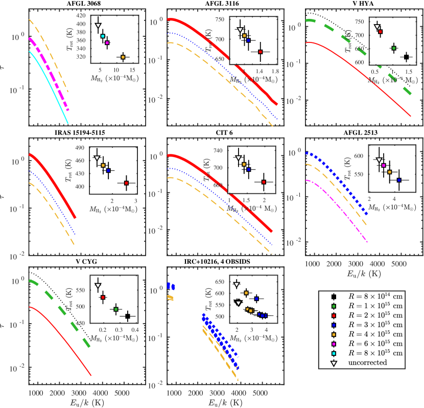
Figure 14: Optical depth at line center ($\tau$) as a function of the energy of the upper level ($E_{\rm u}$). $\tau$ was computed for a range of radii; the characteristic radius adopted ($r_{\rm CO}$, Table 1) is marked with a thick line. In each panel, the inset shows the values of $T_{\rm rot}$ and $M_{\rm H_{2}}$ after the $C_{\tau}$ correction has been applied for the corresponding radii, along with the opacity-uncorrected results (open triangle).

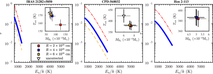
Figure 15: Continued.

In case of optically thick emission, an optical depth correction factor $\rm C_{\tau}$ should be added to the RD to compensate for an underestimation of the mass within the CO-emitting volume. The optical depth at the line center ($\tau$) of a given CO ($J_{\rm u}$-$J_{\rm l}$) transition is:

$$\tau=\frac{A_{\rm ij}\lambda^{3}_{0}N^{\rm col}_{\mathrm{u}}}{8\pi V}\times[e^{(h\nu/kT)}-1]$$ (3)

where $V=v_{\rm exp}\sqrt{\pi}/(2\sqrt{\log 2})\leavevmode\nobreak\ [\rm km\leavevmode\nobreak\ s^{-1}]$ with $v_{\rm exp}$ being the expansion velocity of the gas, $N^{\rm col}_{\mathrm{u}}=N_{\mathrm{u}}/\pi r_{\rm CO}^{2}$ is the column density of the upper level, $A_{\rm ij}$ is the Einstein coefficient for spontaneous emission and $\lambda_{0}$ is the peak wavelength. It follows that the correction factor is written as:

$$C_{\tau}=\frac{\tau}{1-e^{-\tau}}$$ (4)

To compute $C_{\tau}$, we perform a first fit of the RD datapoints, $\ln\left(\frac{N_{\rm u}}{g_{\rm u}}\right)_{0}$, starting with null opacity correction ($\ln C_{\tau}=0$) which yields initial (or opacity-uncorrected) values of $T_{\rm rot}$ and $N_{\rm CO}$. We use these values to calculate $\tau$ and $C_{\tau}$ and to apply the opacity correction, that is, $\ln\left(\frac{N_{\rm u}}{g_{\rm u}}\right)_{1}$ = $\ln\left(\frac{N_{\rm u}}{g_{\rm u}}\right)_{0}+\ln C_{\tau}$. A second fit to $\ln\left(\frac{N_{\rm u}}{g_{\rm u}}\right)_{1}$ is then performed, which renders the so-called opacity-corrected values of $T_{\rm rot}$ and $N_{\rm CO}$ (Table 1).

We want to highlight that, as explained in Goldsmith & Langer (1999), the opacity correction is only reliable for moderate values of the optical depth. For this reason, for all objects in our sample, the minimum acceptable value of $r_{\rm CO}$ used to compute the CO column density is always chosen so that it results in values of $\tau$ close to, but smaller than, unity (Fig. 14). Indeed, the envelope layers where $\tau\sim$1 are the deepest regions observationally accessible, because of the almost null escape probability (1/$C_{\tau}$ $\rightarrow$0) from deeper, optically thicker regions. As seen in Fig. 14, for $r_{\rm CO}$$\la$1$\times 10^{\rm 15}$ cm the opacity of the CO $J$=14-13 line ($E_{\rm u}$=580 K), which is the optically thickest transition in our sample, becomes larger than 1 in all our targets. The expected size of the CO-emitting volume in our sample is discussed in detail in Section. 4.

The optical depth of the line is also sensitive to the expansion velocity of the gas (Eq. 3), which is unconstrained from PACS data and has been assumed to be the terminal expansion velocity of the AGB CSE from the literature (values and references are given in Table 3). In the case of pAGBs and yPNe, we adopt the average expansion velocity of the bulk of the envelope from different previous works. The uncertainty of $v_{\rm exp}$ is normally less than 10%.

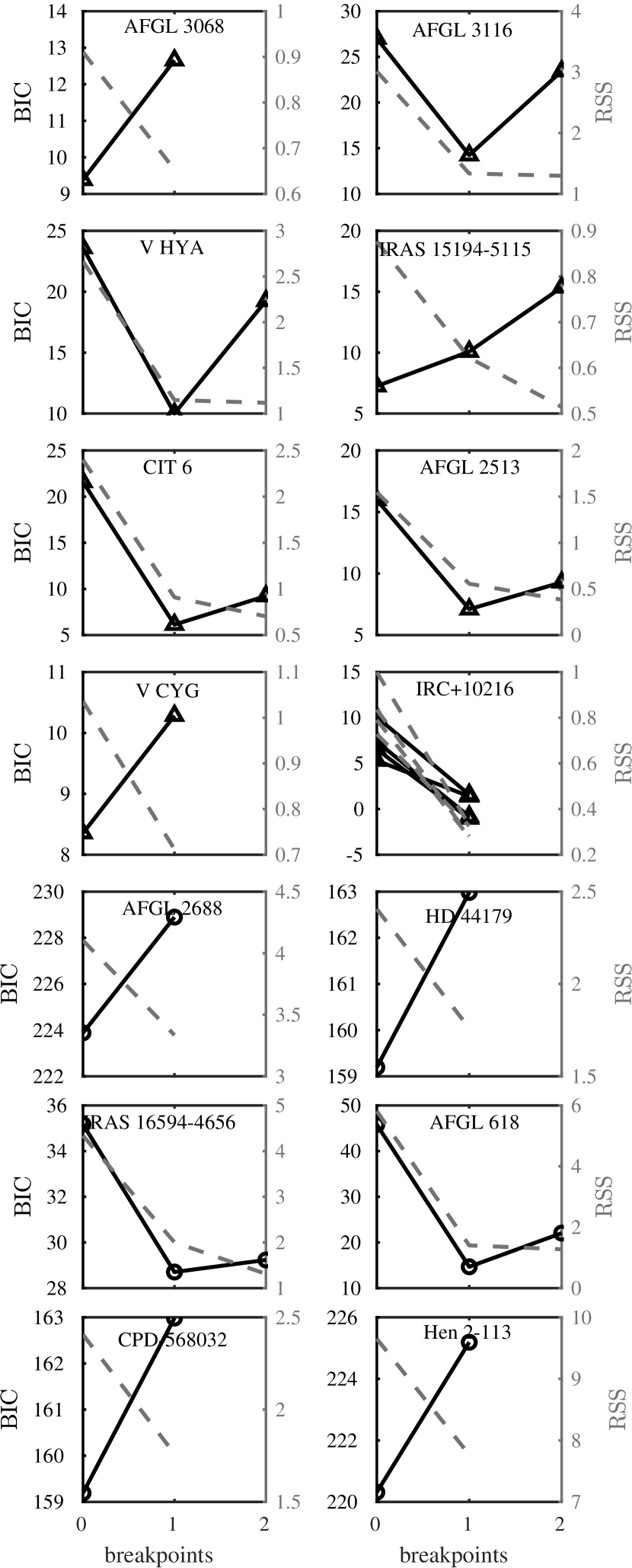
Figure 16: Bayesian information criterion and residual sum of squares as a function of number of breakpoints. The BIC is given by the solid line and the RSS is given by the dashed line. The statistic was not computed for IRAS 21282+5050 due to insufficient number of points.

A.2 Model selection with BIC

Here we describe the method used to automatically find a break point in the linear relation in the rotational diagram using the Bayesian information criterion (BIC).

Our approach concerns the minimization of the RSS (residual sum of squares) by computing the BIC for a range of possible locations of break points. The BIC can be regarded as a rough estimate of the Bayes factor (Schwarz 1978), and it is given by:

$$BIC=n\ln(RSS/n)+k\ln(n)$$ (5)

where a penalty term, $k\ln(n)$, penalizes model complexity depending on the number of parameters $k$ and data points $n$ (see also Maindonald & Braun 2010). We also tested the Akaike’s information criterion (AIC) (Akaike 1974), but we concluded that for this particular application it tends to overfit essentially because the penalty term is smaller. In fact, due to the small number of data points, we are not interested in splitting the rotational diagram too much in order to obtain robust results. It can happen that BIC suggests more than one breakpoint due to the smaller accuracy of the higher $J$ line fluxes, and in that case only the first break point is taken into account. Obvious line blends were excluded upon the computation of both statistics.

Figure 16 shows the BIC test in a graphical way where we see that the BIC curve is usually minimal at 0 or 1 breakpoints. For example for AFGL 2513 it is shown that the residuals of the fit keep decreasing with 2 breakpoints, although this is strongly penalized by the BIC, so a 2-component fit is favored. On the contrary, in AFGL 3068, IRAS 15194-5115 and IRC+10216 a single temperature component suffices to reproduce the data.

We note that these methods do not prove that a double temperature component is physically true, neither they provide an alternative explanation for the trends in the data. They simply highlight hidden patterns in the residuals which can be caused by many effects, being line blend the most obvious among them, or heteroscedasticity.

Appendix B Tables

Table 3: Characterization of PACS observations.

Target name	Alt. name	Class	R.A. (J2000)	DEC (J2000)	OBSID	Obs. date
AFGL 3068	LL Peg	C-rich AGB	$23^{\rm h}19^{\rm m}12^{\rm s}.39$	$17\textordmasculine 11^{\prime}35\arcsec.4$	1342199417 1342199418	2010-06-30
AFGL 3116	LP And	C-rich AGB	$23^{\rm h}34^{\rm m}27^{\rm s}.67$	$43\textordmasculine 33^{\prime}2\arcsec.52$	1342212512 1342212513	2011-01-11
IRC+10216	CW Leo	C-rich AGB	$9^{\rm h}47^{\rm m}57^{\rm s}.41$	$13\textordmasculine 16^{\prime}43\arcsec.60$	1342221889 1342241328 1342245395 1342246381 1342253754 1342255741 1342256262	2011-05-29 2011-10-25 2012-05-05 2012-05-30 2012-10-21 2012-11-21 2012-11-30
IRAS 15194-5115	II Lup	C-rich AGB	$15^{\rm h}23^{\rm m}4^{\rm s}.91$	$-51\textordmasculine 25^{\prime}59\arcsec.0$	1342215685 1342215686	2010-03-10
CIT 6	RW Lmi	C-rich AGB	$10^{\rm h}16^{\rm m}2^{\rm s}.28$	$30\textordmasculine 34^{\prime}18\arcsec.48$	1342197799 1342197800	2010-06-05
AFGL 2513	V1969 Cyg	C-rich AGB	$20^{\rm h}09^{\rm m}14^{\rm s}.25$	$31\textordmasculine 25^{\prime}44\arcsec.9$	1342270010 1342269936	2013-04-14 2013-04-12
V Cyg		C-rich AGB	$20^{\rm h}41^{\rm m}18^{\rm s}.27$	$48\textordmasculine 08^{\prime}28\arcsec.8$	1342208939 1342208940	2010-11-15
V Hya		C-rich AGB	$10^{\rm h}51^{\rm m}37^{\rm s}.25$	$21\textordmasculine 15^{\prime}00\arcsec.3$	1342197790 1342197791	2010-06-05
AFGL 2688	Egg Nebula	C-rich post-AGB	$21^{\rm h}2^{\rm m}18^{\rm s}.74$	$36\textordmasculine 41^{\prime}37\arcsec.68$	1342199233 1342199234	2010-06-26
HD 44179	Red Rectangle	mixed post-AGB	$6^{\rm h}19^{\rm m}58^{\rm s}.22$	$-10\textordmasculine 38^{\prime}14\arcsec.7$	1342220928 1342220929	2011-04-30
IRAS 16594-4656	Water Lily Nebula	mixed post-AGB	$17^{\rm h}03^{\rm m}10^{\rm s}.03$	$-47\textordmasculine 00^{\prime}27\arcsec.7$	1342228414 1342228415	2011-09-10
AFGL 618	CRL 618	C-rich yPNe	$4^{\rm h}42^{\rm m}53^{\rm s}.66$	$36\textordmasculine 6^{\prime}53\arcsec.28$	1342225838 1342225839	2011-08-07
IRAS 21282+5050		C-rich yPNe	$21^{\rm h}29^{\rm m}58^{\rm s}.42$	$51\textordmasculine 3^{\prime}59\arcsec.76$	1342220741 1342223375	2011-05-12 2011-06-30
CPD-568032	Hen 3-1333	mixed yPNe	$17^{\rm h}7^{\rm m}0^{\rm s}.87$	$-56\textordmasculine 54^{\prime}48\arcsec.0$	1342228201 1342228202	2011-09-06
Hen 2-113		mixed yPNe	$14^{\rm h}59^{\rm m}53^{\rm s}.52$	$-54\textordmasculine 18^{\prime}07\arcsec.20$	1342225142 1342225143	2011-08-02

Table 4: Properties of stars and their CSEs taken from the bibliography.

Target name	Var.	$T_{\rm eff}$ (K)	$d$ (pc)	$v_{\rm exp}\leavevmode\nobreak\ \rm(km\leavevmode\nobreak\ s^{-1})$	$\dot{M}\rm\leavevmode\nobreak\ (M_{\sun}\leavevmode\nobreak\ yr^{-1})$		references
AFGL 3068	Mira	2000	1100	13	(0.9, 6) $\times 10^{-5}$	(0.8, 6.8) $\times 10^{-5}$	2, 10, 23, 29
AFGL 3116	Mira	2000	630	14	(4.6, 12) $\times 10^{-6}$	(1, 11.8) $\times 10^{-6}$	2, 10, 23
IRC+10216	Mira	2330	150	14.5	(0.2, 4) $\times 10^{-5}$	(0.05, 3.2) $\times 10^{-5}$	2, 12, 23, 24, 31
IRAS 15194-5115	Mira	2400	500	23	(0.4, 1.5) $\times 10^{-5}$	(0.08, 2.5) $\times 10^{-5}$	2, 10, 13
CIT 6	SRa	2450	440	21	(5, 6) $\times 10^{-6}$	(1.2, 11) $\times 10^{-6}$	2, 10, 23
AFGL 2513	Mira	2500	1760	26	2 $\times 10^{-5}$	(1, 4) $\times 10^{-5}$	6, 14
V Cyg	Mira	2580	271	15	(0.4, 6.3) $\times 10^{-6}$	(0.08, 1.7) $\times 10^{-6}$	2, 10, 15
V Hya	SR/Mira	2650	380	24	(0.25, 6) $\times 10^{-5}$	(0.03, 3) $\times 10^{-5}$	1, 10, 17, 25
AFGL 2688		7250	340	20	(0.7, 2) $\times 10^{-4}$	(0.06, 0.6) $\times 10^{-4}$	3, 8, 19, 27
HD 44179		7750	710	8.3	$10^{-7}$-$10^{-5}$	$10^{-7}$-$10^{-5}$	5, 7, 10, 32
IRAS 16594-4656		10000	1800	14	1 $\times 10^{-5}$	(0.4, 3.7) $\times 10^{-5}$	9, 18
AFGL 618		33000	900	80	(0.3, 2) $\times 10^{-4}$	(0.06, 0.7) $\times 10^{-4}$	4, 16, 26, 27, 30
IRAS 21282+5050		30000	2000	14	(2, 10) $\times 10^{-5}$	(1.5, 7.5) $\times 10^{-5}$	11, 21, 26
CPD-568032		30000	1530	22.6	(1.2-4) $\times 10^{-6}$	(1.2-4) $\times 10^{-6}$	20, 28
Hen 2-113		30900	1230	23	(6.3-8) $\times 10^{-7}$	(6.3-8) $\times 10^{-7}$	20, 28

$\leavevmode\nobreak\ {}^{(1)}$Bergeat & Chevallier (2005), $\leavevmode\nobreak\ {}^{(2)}$Ramstedt & Olofsson (2014), $\leavevmode\nobreak\ {}^{(3)}$Balick et al. (2012), $\leavevmode\nobreak\ {}^{(4)}$Sánchez Contreras et al. (2004), $\leavevmode\nobreak\ {}^{(5)}$Bujarrabal et al. (2016) $\leavevmode\nobreak\ {}^{(6)}$Guandalini et al. (2006), $\leavevmode\nobreak\ {}^{(7)}$Men’shchikov et al. (2002), $\leavevmode\nobreak\ {}^{(8)}$Ishigaki et al. (2012), $\leavevmode\nobreak\ {}^{(9)}$Mishra et al. (2015) $\leavevmode\nobreak\ {}^{(10)}$De Beck et al. (2010), ⁽¹¹⁾Hasegawa & Kwok (2003), $\leavevmode\nobreak\ {}^{(12)}$Cernicharo et al. (2015a),$\leavevmode\nobreak\ {}^{(13)}$Ryde et al. (1999), $\leavevmode\nobreak\ {}^{(14)}$Groenewegen et al. (2002), $\leavevmode\nobreak\ {}^{(15)}$Neufeld et al. (2010), $\leavevmode\nobreak\ {}^{(16)}$Huang et al. (2016), $\leavevmode\nobreak\ {}^{(17)}$Knapp et al. (1997), $\leavevmode\nobreak\ {}^{(18)}$Woods et al. (2005), $\leavevmode\nobreak\ {}^{(19)}$Milam et al. (2009), $\leavevmode\nobreak\ {}^{(20)}$De Marco & Crowther (1998), $\leavevmode\nobreak\ {}^{(21)}$Likkel et al. (1988), $\leavevmode\nobreak\ {}^{(22)}$Bujarrabal et al. (2016), $\leavevmode\nobreak\ {}^{(23)}$Teyssier et al. (2006), $\leavevmode\nobreak\ {}^{(24)}$De Beck et al. (2012), $\leavevmode\nobreak\ {}^{(25)}$Knapp et al. (1999), $\leavevmode\nobreak\ {}^{(26)}$Meixner et al. (1998), $\leavevmode\nobreak\ {}^{(27)}$Bujarrabal et al. (2001), $\leavevmode\nobreak\ {}^{(28)}$Leuenhagen et al. (1996), $\leavevmode\nobreak\ {}^{(29)}$Sánchez Contreras & Sahai (2012), $\leavevmode\nobreak\ {}^{(30)}$Wesson et al. (2010), $\leavevmode\nobreak\ {}^{(31)}$Guélin et al. (2018), $\leavevmode\nobreak\ {}^{(32)}$Bujarrabal & Alcolea (2013)

Table 5: Carriers of some of the spectral lines detected towards our sample of C-rich evolved stars.

Target Name	Molecular						Atomic/ionized				Dust
	CO	HCN	CS	OH	$\rm H_{2}O$	CH+	[OI] $63.18\rm\mu m$	[NII] $121.89\rm\mu m$	[OI] $145.52\rm\mu m$	[CII] $157.74\rm\mu m$	forsterite $69\rm\leavevmode\nobreak\ \mu m$
AFGL 3068	✓	✓	✓		✓
AFGL 3116	✓	✓	✓		✓
IRC+10216	✓	✓	✓		✓
IRAS 15194-5115	✓	✓	✓		✓
CIT 6	✓	✓	✓		✓
AFGL 2513	✓	✓	✓		✓
V Cyg	✓	✓	✓		✓
V Hya	✓	✓	✓		✓
AFGL 2688	✓	✓			✓
HD 44179	✓						✓		✓	✓	✓
IRAS 16594-4665	✓			✓		✓	✓		✓	✓
AFGL 618	✓	✓		✓	✓		✓		✓	✓
IRAS 21282+5050	✓					✓	✓	✓	✓	✓
CPD-568032	✓			✓		✓	✓		✓	✓	✓
Hen 2-113	✓			✓		✓	✓	✓	✓	✓	✓

Table 6: Line fluxes of CO rotational transitions in a sample of C-rich evolved stars.

Transition	$\rm\nu_{\rm rest}\leavevmode\nobreak\ (MHz)$	$\rm\lambda_{\rm rest}\leavevmode\nobreak\ (\mu m)$	$\rm E_{\rm up}/k\leavevmode\nobreak\ (K)$	$\rm A_{ij}\leavevmode\nobreak\ (s^{-1})$			$F\leavevmode\nobreak\ (\rm\times 10^{-16}\leavevmode\nobreak\ W\leavevmode\nobreak\ m^{-2})$
$\rm{}^{12}CO\leavevmode\nobreak\ (\nu=0)$					CIT 6	V Hya	IRAS 15194-5115	AFGL 2513	V Cyg
$J=14\rightarrow$ 13	1611794	185.999	580.497	0.00027	8.9$\pm$0.3	4.3$\pm$0.2	4.3$\pm$0.4	0.88$\pm$0.07	1.8$\pm$0.2
$J=15\rightarrow$ 14	1726603	173.631	663.361	0.00034	7.7$\pm$0.3	4.6$\pm$0.2	3.9$\pm$0.5	0.96$\pm$0.05	1.8$\pm$0.1
$J=16\rightarrow$ 15	1841346	162.812	751.733	0.00041	9.2$\pm$0.5	5.6$\pm$0.2	5.0$\pm$0.3	1.07$\pm$0.06	2.6$\pm$0.1
$J=17\rightarrow$ 16	1956018	153.267	845.608	0.00048	11.3$\pm$0.6	6.1$\pm$0.2	4.9$\pm$0.3	1.29$\pm$0.08	2.3$\pm$0.1
$J=18\rightarrow$ 17	2070616	144.784	944.983	0.00057	9.6$\pm$0.7	5.3$\pm$0.2	3.7$\pm$0.5	0.99$\pm$0.07	2.7$\pm$0.1
$J=19\rightarrow$ 18	2185135	137.196	1049.854	0.00067	8.1$\pm$0.6	5.0$\pm$0.2	4.1$\pm$0.3	0.84$\pm$0.08	2.7$\pm$0.2
$J=20\rightarrow$ 19	2299570	130.369	1160.217	0.00077	16.2$\pm$0.9	8.9$\pm$0.3	7.4$\pm$0.6	1.7$\pm$0.1	3.9$\pm$0.3
$J=21\rightarrow$ 20	2413917	124.193	1276.068	0.00088	11$\pm$1.0	6.4$\pm$0.3	4$\pm$1	1.0$\pm$0.1	2.6$\pm$0.2
$J=22\rightarrow$ 21	2528172	118.581	1397.402	0.00101	10.9$\pm$0.6	5.9$\pm$0.2	4.3$\pm$0.8	1.0$\pm$0.07	2.7$\pm$0.2
$J=23\rightarrow$ 22	2642330	113.458	1524.215	0.00114	16$\pm$2	9$\pm$1	5$\pm$2	1.5$\pm$0.2	4.1$\pm$0.4
$J=24\rightarrow$ 23	2756388	108.763	1656.502	0.00128	11$\pm$2	5.6$\pm$0.5	5$\pm$2∗	0.9$\pm$0.1	1.9$\pm$0.3
$J=25\rightarrow$ 24	2870339	104.445	1794.258	0.00143	9$\pm$1	5.9$\pm$0.5	3.8$\pm$0.8	0.8$\pm$0.1	2.7$\pm$0.4∗
$J=28\rightarrow$ 27	3211519	93.349	2240.286	0.00194	6.8$\pm$0.4	5.3$\pm$0.3	2.5$\pm$0.4∗	0.7$\pm$0.1	1.2$\pm$0.2
$J=29\rightarrow$ 28	3325005	90.163	2399.862	0.00213	11$\pm$1.0	5.3$\pm$0.4	1.6$\pm$0.4	0.8$\pm$0.1	1.8$\pm$0.2
$J=30\rightarrow$ 29	3438365	87.19	2564.879	0.00232	9.7$\pm$0.9	6.4$\pm$0.5∗	3.2$\pm$0.8	1.5$\pm$0.2∗	2.1$\pm$0.4∗
$J=31\rightarrow$ 30	3551592	84.411	2735.331	0.00252	9.8$\pm$0.9	4.9$\pm$0.3	1.7$\pm$0.6	0.9$\pm$0.1	1.6$\pm$0.3
$J=32\rightarrow$ 31	3664684	81.806	2911.209	0.00274	6.1$\pm$0.9	4.1$\pm$0.6	…	0.7$\pm$0.2	1.0$\pm$0.3
$J=33\rightarrow$ 32	3777636	79.359	3092.509	0.00295	5.4$\pm$0.9	5.2$\pm$0.6	…	0.7$\pm$0.2	0.96$\pm$0.3
$J=34\rightarrow$ 33	3890443	77.059	3279.223	0.00318	9$\pm$1	4.6$\pm$0.4	…	0.7$\pm$0.1∗	1.1$\pm$0.3∗
$J=35\rightarrow$ 34	4003101	74.89	3471.344	0.0034	8$\pm$2∗	3.9$\pm$0.8	…	0.8$\pm$0.1∗	1.2$\pm$0.3∗
$J=36\rightarrow$ 35	4115606	72.843	3668.864	0.00364	4.7$\pm$0.9∗	3.2$\pm$0.3	…	…	…
$J=37\rightarrow$ 36	4227953	70.907	3871.775	0.00388	5$\pm$1	3.0$\pm$0.6∗	…	…	…
$J=38\rightarrow$ 37	4340138	69.074	4080.071	0.00412	3.7$\pm$0.4	2.8$\pm$0.3	…	…	…
$J=39\rightarrow$ 38	4452157	67.336	4293.743	0.00437	3$\pm$1∗	2.5$\pm$0.5∗	…	…	…
$J=40\rightarrow$ 39	4564006	65.686	4512.783	0.00461	3.2$\pm$1.0∗	2.9$\pm$0.7	…	…	…
$J=41\rightarrow$ 40	4675679	64.117	4737.183	0.00486	1.1$\pm$0.6∗	1.4$\pm$0.4	…	…	…
$J=42\rightarrow$ 41	4787174	62.624	4966.933	0.00511	2$\pm$1∗	0.9$\pm$0.5∗	…	…	…
$J=43\rightarrow$ 42	4898485	61.201	5202.026	0.00536	3.3$\pm$0.9∗	1.8$\pm$0.4∗	…	…	…
$J=44\rightarrow$ 43	5009608	59.843	5442.452	0.00561	1.7$\pm$0.6	1.9$\pm$0.5	…	…	…
$J=45\rightarrow$ 44	5120539	58.547	5688.201	0.00585	…	…	…	…	…

Table 7: Continued.

AFGL 3068	AFGL 3116	AFGL 618	HD 44179	IRAS 16594-4656	AFGL 2688	Hen 2-113	CPD-568032	IRAS 21282+5050
2.1$\pm$0.2	2.7$\pm$0.2	39$\pm$1	0.4$\pm$0.1	4.1$\pm$0.1	41$\pm$1	2.24$\pm$0.09	2.4$\pm$0.1	2.96$\pm$0.06
2.1$\pm$0.2	2.9$\pm$0.2	33$\pm$1	0.39$\pm$0.09	4.1$\pm$0.1	36$\pm$1	2.16$\pm$0.07	2.3$\pm$0.1	2.92$\pm$0.05
2.3$\pm$0.1	2.8$\pm$0.1	40$\pm$1	0.4$\pm$0.1	3.9$\pm$0.3	33$\pm$1	2.3$\pm$ 0.5	2.2$\pm$0.1	2.42$\pm$0.06
2.5$\pm$0.2	4.1$\pm$0.3	37$\pm$1	0.53$\pm$0.09	3.2$\pm$0.1	26$\pm$1	2.3$\pm$ 0.1	2.0$\pm$0.07	1.63$\pm$0.04
2.7$\pm$0.3	3.5$\pm$0.2	38$\pm$1	0.6$\pm$0.1	2.76$\pm$0.06	25$\pm$1	2.1$\pm$ 0.1	1.9$\pm$0.1	1.04$\pm$0.07
2.5$\pm$0.2	3.0$\pm$0.2	39$\pm$2	0.45$\pm$0.09	2.42$\pm$0.01	22$\pm$1	2.0$\pm$ 0.1	1.6$\pm$0.1	0.9$\pm$0.1
3.9$\pm$0.2	6.1$\pm$0.4	44$\pm$1	0.4$\pm$0.1	2.5$\pm$0.1	24$\pm$1	2.2$\pm$ 0.1	2$\pm$0.2	0.59$\pm$0.09
2.3$\pm$0.3	4.3$\pm$0.5	34$\pm$2	0.4$\pm$0.1	2.8$\pm$0.1	17$\pm$1	2.0$\pm$ 0.1	1.7$\pm$0.2	0.50$\pm$0.08
2.7$\pm$0.2	3.6$\pm$0.2	36$\pm$2	0.7$\pm$0.1	2.2$\pm$0.2	18$\pm$1	2.4$\pm$ 0.3	1.3$\pm$0.2	…
2.5$\pm$0.6	4.6$\pm$0.9	46$\pm$2	0.4$\pm$0.2	2.7$\pm$0.1	14$\pm$2	2.2$\pm$0.3	1.9$\pm$0.2	…
1.6$\pm$0.4	3.7$\pm$0.6	28$\pm$2∗	…	1.9$\pm$0.1	11$\pm$2	1.2$\pm$0.2	1.0$\pm$0.2	…
1.3$\pm$0.5	3.4$\pm$0.2	31$\pm$2	…	2.1$\pm$0.2	6$\pm$2	1.6$\pm$0.2	1.2$\pm$0.3	…
1.2$\pm$0.3	3.2$\pm$0.3	21$\pm$1	…	1.6$\pm$0.1	6$\pm$1	0.7$\pm$0.2	0.9$\pm$0.1	…
1.9$\pm$0.4∗	3.3$\pm$0.3	25$\pm$1	…	1$\pm$2∗	11$\pm$2∗	…	bad fit	…
…	4.5$\pm$0.5∗	20$\pm$1	…	1.3$\pm$0.1	bad fit∗	…	…	…
…	2.9$\pm$0.3	26$\pm$2	…	4.9$\pm$0.8∗	4$\pm$2	…	…	…
…	2.0$\pm$0.2	17$\pm$2	…	0.9$\pm$0.1	…	…	…	…
…	2.4$\pm$0.5	15$\pm$2∗	…	0.8$\pm$0.8∗	…	…	…	…
…	2.4$\pm$0.7∗	16$\pm$2	…	0.7$\pm$0.1	…	…	…	…
…	2.2$\pm$0.4	16$\pm$2	…	0.8$\pm$0.1∗	…	…	…	…
…	2.3$\pm$0.5	11$\pm$1	…	…	…	…	…	…
…	3$\pm$1∗	13$\pm$3∗	…	…	…	…	…	…
…	1.3$\pm$0.2∗	11$\pm$1	…	…	…	…	…	…
…	0.9$\pm$0.3	6$\pm$5	…	…	…	…	…	…
…	0.9$\pm$0.3	5$\pm$2	…	…	…	…	…	…
…	…	10$\pm$2	…	…	…	…	…	…
…	…	37$\pm$20∗	…	…	…	…	…	…
…	…	9$\pm$3	…	…	…	…	…	…
…	…	6$\pm$2	…	…	…	…	…	…
…	…	3$\pm$2	…	…	…	…	…	…

Table 8: CO line fluxes of seven observations of IRC+10216. Asterisks flag known line blends.

Transition	$\rm\nu_{\rm rest}\leavevmode\nobreak\ (MHz)$	$\rm\lambda_{\rm rest}\leavevmode\nobreak\ (\mu m)$	$\rm E_{\rm up}/k\leavevmode\nobreak\ (K)$	$\rm A_{\rm ij}\leavevmode\nobreak\ (s^{-1})$				$F\leavevmode\nobreak\ \rm(\rm\times 10^{-16}\leavevmode\nobreak\ W\leavevmode\nobreak\ m^{-2})$
$\rm{}^{12}CO\leavevmode\nobreak\ (\nu=0)$					OD 745	OD 894	OD 1087	OD 1113	OD 1257	OD 1288	OD 1296
$J=14\rightarrow$ 13	1611794	185.99	580.5	0.00027	85$\pm$3	98$\pm$10	92$\pm$4	90$\pm$5	97$\pm$3	86$\pm$8	100$\pm$3
$J=15\rightarrow$ 14	1726603	173.63	663.36	0.00034	74$\pm$5	103$\pm$13	80$\pm$6	108$\pm$30	82$\pm$5	88$\pm$8	80$\pm$5
$J=16\rightarrow$ 15	1841346	162.81	751.73	0.00041	89$\pm$4	100$\pm$24	93$\pm$3	93$\pm$12	78$\pm$2	89$\pm$12	79$\pm$3
$J=17\rightarrow$ 16	1956018	153.27	845.61	0.00048	92$\pm$7		99$\pm$7		92$\pm$7		89$\pm$6
$J=18\rightarrow$ 17	2070616	144.78	944.98	0.00057	82$\pm$7		85$\pm$6		110$\pm$5		102$\pm$5
$J=28\rightarrow$ 27	3211519	93.35	2240.29	0.00194	69$\pm$2	104$\pm$18	97$\pm$3	104$\pm$18	64$\pm$2	59$\pm$15	62$\pm$2
$J=29\rightarrow$ 28	3325005	90.16	2399.86	0.00213	72$\pm$4	124$\pm$15	95$\pm$6	124$\pm$15	80$\pm$5	78$\pm$10	77$\pm$5
$J=30\rightarrow$ 29	3438365	87.19	2564.88	0.00232	55$\pm$7	82$\pm$12	82$\pm$9	82$\pm$12	72$\pm$6	50$\pm$9	55$\pm$4
$J=31\rightarrow$ 30	3551592	84.41	2735.33	0.00252	57$\pm$7	108$\pm$11	101$\pm$9	108$\pm$11	52$\pm$5	60$\pm$6	55$\pm$5
$J=32\rightarrow$ 31	3664684	81.81	2911.21	0.00274	37$\pm$8	54$\pm$18	68$\pm$6	54$\pm$18	47$\pm$5	26$\pm$11	39$\pm$4
$J=33\rightarrow$ 32	3777636	79.36	3092.51	0.00295	43$\pm$8	80$\pm$15	79$\pm$10	80$\pm$15	42$\pm$5	39$\pm$7	40$\pm$4
$J=34\rightarrow$ 33	3890443	77.06	3279.22	0.00318	38$\pm$8		64$\pm$9		30$\pm$5		35$\pm$5
$J=35\rightarrow$ 34	4003101	74.89	3471.34	0.0034	34$\pm$8∗		64$\pm$9∗		39$\pm$8∗		38$\pm$7∗
$J=36\rightarrow$ 35	4115606	72.84	3668.86	0.00364	19$\pm$7		32$\pm$9		23$\pm$5		18$\pm$4
$J=37\rightarrow$ 36	4227953	70.91	3871.78	0.00388	20$\pm$6		45$\pm$10		20$\pm$6		22$\pm$6

Appendix C Supplement figures