Efficient treatment of model discrepancy by Gaussian Processes - Importance for imbalanced multiple constraint inversions

Abstract

Mechanistic simulation models are inverted against observations in order to gain inference on modeled processes. However, with the increasing ability to collect high resolution observations, these observations represent more patterns of detailed processes that are not part of a modeling purpose. This mismatch results in model discrepancies, i.e. systematic differences between observations and model predictions. When discrepancies are not accounted for properly, posterior uncertainty is underestimated. Furthermore parameters are inferred so that model discrepancies appear with observation data stream with few records instead of data streams correponding to the weak model parts. This impedes the identification of weak process formulations that need to be improved. Therefore, we developed an efficient formulation to account for model discrepancy by the statistical model of Gaussian processes (GP). This paper presents a new Bayesian sampling scheme for model parameters and discrepancies, explains the effects of its application on inference by a basic example, and demonstrates applicability to a real world model-data integration study.

The GP approach correctly identified model discrepancy in rich data streams. Innovations in sampling allowed successful application to observation data streams of several thousand records. Moreover, the proposed new formulation could be combined with gradient-based optimization. As a consequence, model inversion studies should acknowledge model discrepancies, especially when using multiple imbalanced data streams. To this end, studies can use the proposed GP approach to improve inference on model parameters and modeled processes.

• December 2018

Keywords: Bayesian, multiple constraint, Gaussian process, model discrepancy, imbalanced data streams

1 Introduction

The increased availability of high-resolution observation data streams in many sciences (Luo et al., 2011) allows constructing and evaluating detailed process models (Keenan et al., 2011). Often, the data supports higher detail than required by the modeling purpose. Mismatch in detail between observations and model leads to model discrepancy: systematic differences between the observed process and the prediction of a calibrated model. Model discrepancy is often ignored in model-data integration studies, or it is treated as part of a Gaussian residual term (Tarantola, 2005). Yet, model discrepancies cause correlation in model-data residuals that are not accounted for by correlations in observations. Such unaccounted correlations lead to overconfident estimates of parameters and predictions (Weston et al., 2014). They can also lead to biased parameter estimates, especially when used with imbalenced data streams, i.e. streams that strongly differ by their number of records (Wutzler and Carvalhais, 2014). A treatment for model discrepancy, hence, is important for model calibration.

Researchers in numerical weather prediction early acknowledged the importance of accounting for correlations in model data residuals and developed methods for estimating those observations (Bormann et al., 2003; Healy and White, 2005; Weston et al., 2014). If a background, i.e. a previous ensemble of model predictions, is available and if certain conditions are fulfilled, the covariance matrix can be estimated using both the predicions based on the background and predictions based on the posterior sample (Desroziers et al., 2005; Waller et al., 2014). However, it is hard for this approach to account for tradeoffs among imbalanced data streams, because all ensemble members are based on the same estimate of the covariance matrix. An approach that is suitable for trade-offs should allow discrepancies and correlations matrices to differ across parameter samples. A promising alternative approach is to represent discrepancy explicitly as a statistical distribution called Gaussian process (GP) (Kennedy and O’Hagan, 2001; Brynjarsdóttir and O’Hagan, 2014), which is further described in section 2.1.

Adding additional constraints or data streams of various types holds the promise to constrain different aspects of the model (Richardson et al., 2010; Ahrens et al., 2014). The addition of sparse data stream, i.e. data sets of relatively few records, has, however, only neglibile influence on the model fit if no additional weights are applied. Model discrepancy is allocated preferentially to sparse data streams. This preferential allocation leads to complications in identifying model deficiendies in studies using imbalanced data streams, i.e. streams that strongly differ in their number of records (Wutzler and Carvalhais, 2014).

The objectives of this study center around a better allocation of model discrepancy and improved inference on modeled processes in inversion studies using imbalanced data streams. The objectives are to

• demonstrate the problem of preferential allocation of model discrepancy to sparse data streams,

• present an efficient sampling formulation where model discrepancy is represented as a Gaussian processes (GP),

• demonstrate the ability of the GP approach to better allocate discrepancy helping identification of which modelled processes need improvement.

• demonstrate the applicability of the GP approach to real world problems involving rich data streams.

This study focuses on deterministic models and parameter estimation by batch data assimilation (Zobitz et al., 2011). The initial state is assumed to be given or part of the vector of parameters to estimate. For each proposed parameter vector, there is a unique model prediction for each observation.

In addition, the study focuses on approaches that combine evidence from all data streams into a scalar valued objective function. The data stream likelihoods are combined by their product, i.e. saying how likely the first constraint “AND” the other constraints are, given a set of parameters. This approach differs from multi-objective optimization where the trade-offs are explored by using a vector-valued objective function, and the user has to specify additional information on how to select among different trade-offs (Miettinen, 1999). The Bayesian approach employed in this study corresponds to using the information content of the different streams to determine the location in the pareto front in case of trade-offs.

The paper is structured as follows. The remainder of this section visually introduces the approach of explicitly representing model discrepancy via a GP and how this apoproach affects posterior predictions. Section 2 gives a mathematical introduction to the GP approach and introduces both the basic example and the real-world ecosystem case used in the remainder of the paper. Section 3.1 demonstrates the effects using the GP approach on model inference with imbalanced data streams, by using a basic example with two scenarios: one that ignores model discrepancies and another one that explicitly models discrepancy as a GP. Section 3.2 briefly demonstrates the applicability of the GP approach to a real world inversion problem, the Dalec-Howland case. Section 4 discusses how several problems were tackled and what we learned.

The concept of representing model discrepancy as a GP is visualized in Figure 1, which displays two examples of model predictions and model discrepancies against observations. The surrogate process of the example, i.e. the process generating the synthethic data, consists of a linear part plus an oscillating part. The model only accounts for the linear part, but is used to gain inferences on the slope. Model discrepancy constitutes the other oscillating part. It is treated as a smooth sequence of values at observation locations, $x$, and is represented as a GP. It is extremely large, here, for visualization purposes. Its uncertainty is reflected by several samples from the GP (several squiggly lines in Figure 1) conditioned on observed model-observation differences at some supporting locations (triangles in Figure 1). Note that differences between observation and process predictions, i.e. model plus discrepancy, are similar across predictions by different model parameters (top and bottom panels).

Figure 1: Process predictions (squiggly lies) that approximate observations (dots) are the sum of a model prediction, $\mathbf{g}$ (straight line) and several realizations of model discrepancy $\boldsymbol{\delta}$: $\mathbf{o}\sim N(\mathbf{g}(\boldsymbol{\theta})+\boldsymbol{\delta},\sigma^{2}_{\epsilon})$. Process predictions (top and bottom panel) obtained by different parameters (model parameters $\boldsymbol{\theta}=(intersept,slope)^{T}$, and correlation length $\psi$) are more similar than the corresponding model predictions. The respective two Gaussian process (GP) models of discrepancies have been trained on a subset of data at supporting locations indicated by triangles.

The GP approach affects inference mainly by an increased estimate of prediction uncertainty (Figure 2). The inversion with the ignore scenario, which does not acknowledge correlation among model-data residuals, overestimates information content in the observations and hence overestimates precision of posterior estimates. Contrary, the GP approach strongly reduces correlations among residuals between observations process predictions, i.e. model predictions plus discrepancies. At the same time, it yields in a similar likelihood for a broader range of model parameters (compare rows in Figure 1), and hence increases the estimate of uncertainty.

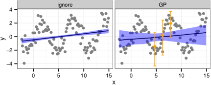
Figure 2: Uncertainty estimates of predictions change when accounting for correlations due to model discrepancy. Sampling the linear part of the example data (dots, same as in Figure 1) underestimated prediction uncertainty when ignoring model discrepancy (left), as denoted by the narrow shaded 95% confidence band. Representing discrepancy as a Gaussian process (GP) (right) increased the estimate of uncertainty. In addition, the representation allowed inference on process predictions ($\mathbf{g}_{i}(\boldsymbol{\theta})+\boldsymbol{\delta}_{i}$), as denoted by the 95% confidence interval whiskers.

2 Methods

2.1 modeling discrepancy as a Gaussian process (GP)

The vector of observations $\mathbf{o}$ of one data stream is modelled as the sum of the deterministic model prediction $\mathbf{g}$, an unknown smooth correlated vector of model discrepancy $\boldsymbol{\delta}$, and observation error $\boldsymbol{\epsilon}$ as (Kennedy and O’Hagan, 2001):

$$\mathbf{o} =\mathbf{g}(\boldsymbol{\boldsymbol{\theta}})+\boldsymbol{\delta}+\boldsymbol{\epsilon}$$ (1a)

$$\boldsymbol{\epsilon} \sim N(\mathbf{0},\boldsymbol{\Sigma})$$ (1b)

$$\boldsymbol{\delta} \sim GP\left(\mathbf{0},K\right).$$ (1c)

The model prediction $\mathbf{g}$ depends on parameter vector $\boldsymbol{\boldsymbol{\theta}}$, whose distribution is to be estimated. The model can be a simple regression function or a complex deterministic dynamical simulation model. The observation error $\boldsymbol{\epsilon}$ is assumed to be Gaussian noise, often with the additional assumptions of independent errors: $\boldsymbol{\Sigma}=\sigma^{2}_{\epsilon}\mathbf{I}$. The unknown vector of the model discrepancy is modelled as as GP. It accounts for the additional correlations in model-data residuals due to model discrepancy. Here, the GP uses a squared exponential covariance function, $K(x_{p},x_{q})=\sigma^{2}_{d}exp(-(x_{p}-x_{q})^{2}/\psi^{2}+\sigma^{2}_{\epsilon}\delta_{pq})$, where the Kronecker delta $\delta_{pg}$ equals one for $p=q$ and zero otherwise. The covariance function has two hyperparameters: correlation length $\psi$ that controls the smoothness of the model discrepancy across neighboring locations, and signal variance $\sigma^{2}_{d}$ that controls the amplitude of the discrepancies varying around the expected value of zero (Rasmussen and Williams, 2006). The approach is applicable also for different assumptions about the measurement error or the covariance structure of the model discrepancies.

2.2 Dimensionless model discrepancy variance

When dealing with multiple data streams, the different units of model discrepancy variance $\sigma^{2}_{d}$ of different streams hinder the comparison of model error. For example one stream may report weights of soil carbon and the other fluxes of carbon dioxide per day. Here, we propose normalizing discrepancy variance for stream, $k$, by the mean variance of observation uncertainty,

$$\sigma^{2}_{k}=\sigma^{2}_{d,k}/\sigma^{2}_{\epsilon,k}.$$ (1b)

The unitless quantity $\sigma^{2}_{k}$ allows comparing model discrepancy across streams. For example, one can state that model discrepancy in stream $k_{1}$ is double the model discrepancy of stream $k_{2}$, although they report different qualities.

2.3 Parameters sampling

The parameters to estimate comprise the vector of model parameters, $\boldsymbol{\boldsymbol{\theta}}$, and for each data stream, $k$, the two scalar hyperparameters $\sigma^{2}_{k}$, and $\psi_{k}$. Variance of observations uncertainty, $\sigma^{2}_{\epsilon}$, is assumed to be known in this study. This section motivates several choices of the sampling strategy, while A reportes the details of the sampling.

Sampling used the Block-at-a-Time Metropolis-Hastings algorithm (Hastings, 1970; Chib and Greenberg, 1995; Gelman et al., 2003). Each signal variance, $\sigma^{2}_{k}$, was sampled from an inverse Gamma distribution. All the other parameters were sampled by Metropolis steps. A Metropolis step can be used to obtain a sample from a random variable for which probability density can be evaluated up to a normalizing constant (Metropolis et al., 1953; Hastings, 1970; Andrieu et al., 2003). One Metropolis step was applied for each hyperparameter $\psi_{k}$ and another Metropolis step was applied for model parameter vector $\boldsymbol{\boldsymbol{\theta}}$. Proposals of new parameter vectors were generated by using differential evolution Markov chain algorithm (ter Braak and Vrugt, 2008).

We used a subset of observation locations, called the supporting locations (triangles in Figure 1), for training the GP model of discrepancies. The usage of a subset improved computational efficiency and prevent numerical singularity, because the resulting matrices were smaller and less prone to numerically singularity (Brynjarsdóttir and O’Hagan, 2014).

In addition, we treated model discrepancies at supporting locations, $\boldsymbol{\delta}_{s}$, as latent variables instead of including them in the set of estimated parameters for two reasons. First, the spacing of the supporting points should adapt to the correlation length to avoid numerical instabilities, and hence the number and location of these supporting locations varied. Second, this treatment dimished the problem of high rejection rate in the Metropolis step and the slow mixing of the parameters, which occurs with sampling that is conditioned on discrepancies (Brynjarsdóttir and O’Hagan, 2014). Furthermore, the resulting formulation can also be used with non-sampling based optimization methods, e.g. gradient-based methods that require a smaller number of model evaluations.

2.4 The basic example

A basic synthethic example demonstrates the problem with imbalanced multiple data streams.

Consider the chemical reaction that oxidizes organic carbon in soil and evolves carbon dioxide ($CO_{2}$). The $CO_{2}$ production rate was monitored over a week, i.e. roughly 1000 times, and found to increase with temperature. For the same site the content of organic matter has been measured september each year in 10 years together with the cumulative amount of $CO_{2}$ produced over two weeks. The cumulated $CO_{2}$ production increased with organic matter content, i.e. the amount of available reactant.

We modeled the corresponding two data streams $\mathbf{o}_{\mathrm{rich}}$ ($n_{\mathrm{rich}}=1000$) and $\mathbf{o}_{\mathrm{sparse}}$ ($n_{\mathrm{sparse}}=10$) of such a system by a surrogate physical process (Reich and Cotter, 2015). The covariates of organic matter content ($\mathbf{x}_{\mathrm{sparse}}$) and temperature ($\mathbf{x}_{\mathrm{rich}}$) were sampled from uniform distributions as $\sim\mathcal{U}(0.5,1.5)$ and $\sim\mathcal{U}(0.7,1)$, respectively.

For demonstration purposes we use a simple linear model, that depends on parameters $a$,$b$, and $c$ as,

$$\hat{\mathbf{o}}_{\mathrm{sparse}}(a,b) =a\,\mathbf{x}_{\mathrm{sparse}}+b\,\overline{x}_{\mathrm{rich}}/10.$$ (1ca)

$$\hat{\mathbf{o}}_{\mathrm{rich}}(a,b,c) =a\,x_{1,\mathrm{sparse}}+b\,\left(\mathbf{x}_{\mathrm{rich}}-\mathrm{c}\right).$$ (1cb)

The example is set up in a way so that the the spread in the prediction of the sparse data stream, $\mathbf{o}_{\mathrm{sparse}}$, mainly depends on the covariates $\mathbf{x}_{\mathrm{sparse}}$. This is because the process description (1ca) uses a single aggregated value $\overline{x}_{\mathrm{rich}}$, of the covariates of the rich data stream, specifically average september temperature. The spread in the rich data stream $\mathbf{o}_{\mathrm{rich}}$, on the other hand, mainly depends on covariates, $\mathbf{x}_{\mathrm{rich}}$. This is because the process description (1cb) only uses a single value, $x_{\mathrm{1,sparse}}$, of the covariates of the rich data stream, specifically the organic matter content at the year of the measurement campaign.

The surrogate physical process, $\mathbf{o}^{*}$, was generated by running the model with parameters $a^{*}=1$ and $b^{*}=2$, and bias variable $c^{*}=0.3$. Next, observations, $\mathbf{o}$, were generated by adding Gaussian noise to $\mathbf{o}^{*}$ with standard deviation of 4% and 3% of the mean of $\mathbf{o}^{*}_{\mathrm{sparse}}$ and $\mathbf{o}^{*}_{\mathrm{rich}}$, respectively.

Using the generated observations and covariates, the posterior density of parameters $a$ and $b$ were sampled by different scenarios of model inversions. In order to demonstrate the transfer of model uncertainty, all scenarios used a model that slightly differed from the data-generating model. Specifically they used a value of the fixed bias parameter in the process description of the rich data stream (1cb) of $c=0.1$, instead of $c^{*}=0.3$. This bias parameter represents a difference between measured air temperature and the top soil temperature at the site of respiration.

2.5 The real world ecosystem example

The real world example inversely estimated 15 parameters and initial conditions of the process-based ecosystem model of carbon dynamics, the Data Assimilation Linked Ecosystem Carbon (DALEC) (Williams et al., 2005). Observations comprised 10-years of daily eddy covariance-based net ecosystem exchange (NEE) (Hollinger et al., 2004; Hollinger and Richardson, 2005), soil respiration, and litterfall at the Howland forest. While data streams of NEE and respiration had about 2000 observations, litterfall had only one record for each of the 10 years. For demonstration purposes, here, we used estimates of observation uncertainties that were reduced by 25% compared to the original estimates for each data stream. Original estimates of observation error were specified as a function that increased with the magnitude of the fluxes. We applied those functions to the model prediction instead of the observed value in order to prevent preferential fit to low fluxes. Further details of the model inversion settings are described in (Wutzler and Carvalhais, 2014).

3 Results

First, the results of the basic example illustrate the consequences applying several analyses that differ by their treatment of model discrepancy. Second, the ecosystem example demonstrates the applicability of the GP approach to more demanding real world inversion settings.

3.1 Basic example

The inversion of the basic example model (Section 2.4) resulted in different estimates of posterior density of model parameters and in different estimates of predictive posterior density of process values (Figure 3) when using different sampling scenarios (Table 1)

Table 1: Scenarios of model inversions.

Sampling scenario	Description	Section
ignore	ignoring model discrepancy	3.1.1
GP	GP for each stream’s model discrepancy	3.1.2

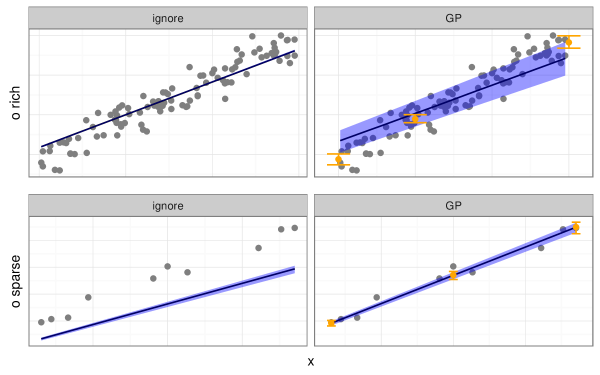
Figure 3: Predictive posterior of the basic example: Ignoring model discrepancy (left) leads to allocation of model discrepancy to the sparse observations, as seen by the misfit between observations (dots) and median model predictions (line inside shaded 95% confidence band). Contrary, representing discrepancies by a GP (right) correctly allocates discrepancy to a slightly worse fit of the biased rich observations. The distribution of process predictions (vertical 95% confidence whiskers) hint to the form of the deficiency in the process formulation.

3.1.1 Analysis without accounting for model discrepancy

With the ignore scenario, model discrepancy was assumed to be the zero vector, $\boldsymbol{\delta}=\mathbf{0}$. The Likelihood of the observations conditioned on model parameters $\boldsymbol{\theta}$ was to the usual formulation derived from the assumption of normally distributed observation errors (Tarantola, 2005).

$$p_{\mathrm{indep}}(\boldsymbol{\theta}|\mathbf{o}) =C_{1}\,p(\mathbf{o}|\boldsymbol{\theta})\,p(\boldsymbol{\theta}).$$

$$\mathrm{log}\left(p_{\mathrm{indep}}(\boldsymbol{\theta}|\mathbf{o})\right) =C_{2}-1/2\sum_{k}S_{k}(\mathbf{o}_{k}|\boldsymbol{\theta})+\mathrm{log}\,p(\boldsymbol{\theta}).$$ (1cd)

$$S_{k}(\mathbf{o}_{k}|\boldsymbol{\theta},\boldsymbol{\delta})=\mathbf{d}^{T}\boldsymbol{\Sigma}^{-1}\mathbf{d}=\sum_{i_{k}}\frac{\mathbf{d}_{i_{k}}^{2}}{\sigma_{\epsilon,i_{k}}^{2}},$$ (1ce)

$$\mathbf{d}_{k}=\mathbf{o}_{k}-\left[\mathbf{g}_{k}(\boldsymbol{\theta})+\boldsymbol{\delta}_{k}\right]$$ (1cf)

where $C_{1}$ and $C_{2}$ are constants, which cancel in the Metropolis decision, and $i_{k}$ iterates across all record numbers in stream $k\in\{rich,sparse\}$, $S_{k}$ is a cost, and $\mathbf{d}_{k}$ is the vector of observation-process residuals.

The infererred uncertainty of the process prediction was very low, indicated by the thin 95% confidence band of the model predictions (first column of Figure 3). Moreover, the introduced model deficiency appeared in the sparse data stream instead of the rich data stream.

By ignoring the model discrepancies, also the additional correlation among model data residuals were ignored. Hence with this scenario, the uncertainty was largely underestimated. Moreover, the results incorrectly suggested that the model fails to predict the sparse data stream, and that the corresponding process description should be refined. Instead, we had introduced the model deficiency in the process description corresponding to the rich data stream (Section 2.4).

3.1.2 Analysis with representing model discrepancy as a GP

With the GP scenario, model discrepancies were represented by a separate GP for each stream. Note that there was an additional term, $-1/2\,\hat{\boldsymbol{\delta}}_{s,k}\mathbf{K}_{ss,k}^{-1}\hat{\boldsymbol{\delta}}_{s,k}$, in the log-density of the parameters (1cs - 1cv) compared to the ignore scenario (3.1.1), effectively penalizing large model discrepancies.

The infererred uncertainty of the process corresponding to the rich observations increased compared to the ignore scenario (Figure 3). The magnitude of model discrepancies in the sparse data stream strongly declined, while the magnitude of model discrepancies in the rich data stream only slightly increased.

The GP scenario helped to tackle both problems: first, the underestimation of posterior variance and second, the unbalanced allocation of model discrepancies.

3.1.3 Analysis using a gradient-based optimization

The optimum parameter set can be found by a gradient-based maximization of the probability densitiy (3.1.1). Here, we used the Broyden-Fletcher-Goldfarb-Shanno (BFGS) method of (Nash, 1990), as implemented by the optim function in the R stats package (R Core Team, 2016). A first order estimate of parameter uncertainty was obtained from the Hessian matrix at the optimum.

Alternatively, the optimum parameter set can be found by maximization of the GP-based density (1cs). In order to maximise this density, we had to a priori specify the parameters of the GP, i.e. supporting locations, correlation length, $\psi_{k}$, and signal variance, $\sigma^{2}_{d,k}$. We specified conservative values based on the results of the optimization that ignored discrepancies (Figure 4 left), where the magnitudes of the model discrepancies exceeded the observation uncertainty, while the correlations spanned the entire range of the data. Specifically, we specified four equidistant supporting points, a correlation length of one-third of the range of the respective covariate, and a signal variance based on 1.5 times the observation uncertainty for all data streams.

Figure 4: Predictive posterior based on a gradient-based optimization of the basic example reveals similar changes on applying the GP-based formulation as with the sampling based inversion (Figure 3). The GP-based inversion (right) correctly allocates discrepancy to the biased rich observations, as seen by the misfit between observations (dots) and median model predictions (line inside shaded 95% confidence band).

The results with gradient-based optimization changed in a similar way as in the sampling-based inversions when representing model discrepancy by a GP. The estimates of the prediction uncertainty increased, while the model discrepancy in the sparse data stream almost disappeared (Figure 4).

3.2 Real world ecosystem example

Model inversions of the 15 DALEC parameters using datastreams with thousands of records was computationally more expensive, both in terms of required model runs and in terms of computing the inverse of the discrepancy correlation matrix. Despite the improved GP sampling formulation, mixing was not as good as expected and we had to increase the thinning interval up to 48. The slowest mixing was observed for correlation length parameters. Chains converged to the limiting distribution after about 2000 samples (C).

When ignoring model discrepancies, posterior distribution of parameters were estimated in such a way that predictions beyond the calibration period lead to very low uncertainty of predictions of the rich data streams of NEE and soil respiration (first column in Figure 5). With the GP scenario the predicted uncertainty increased (second column in Figure 5). This was similar to the results of an inversion based on the parameter blocks approach (Wutzler and Carvalhais, 2014) (shown for comparison in third column of Figure 5).

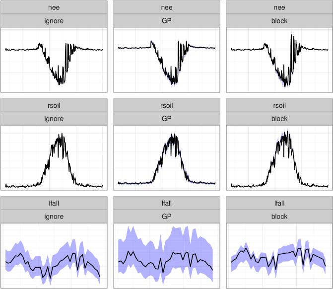
Figure 5: Long term (40 years) future predictive posterior of the DALEC ecosystem example show a more realistic estimation of prediction uncertainty (shaded 95% confidence bands) with the GP and the block approach. Ignoring discrepancy (left) leads to overconfident estimates, as seen by the overplotting of the confidence interval by the median model prediction in the rich NEE and respiration data streams (two top rows, where only the 40^th year is shown). While the GP approach (middle column) leads to increased uncertainty of both rich and sparse data streams, the block approach (right) balances the allocation of uncertainty away from the sparse litterfall stream (bottom row) towards the rich data streams.

The marginal parameter distributions estimated by the GP scenario were mostly broader than the estimates of the ignore and the blocks scenario. Moreover, the GP scenario estimated higher turnover rates (Tl, Tf, Tlab) and lower temperature sensitivity (Et) (C).

The GP inversion estimated the largest model discrepancies for soil respiration (Figure 6), at about double the discrepancy of all the other data streams. The overall magnitude was, however, small with only less than 10% of average observation uncertainty of the corresponding data stream. The DALEC model well captured the patterns in the observations and there was only a negligible trade-off between several constraining data streams.

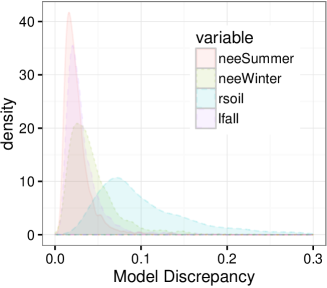
Figure 6: Distribution of discrepancy variance in Howland example was only a small fraction of corresponding variance of observation uncertainty (see Equation 1b). Such a finding increases confidence in the application of the DALEC model.

4 Discussion

The discussion highlights three main points. Section 4.1 discusses how the GP approach can solve problems associated with imbalanced data streams. Next, section 4.2 discusses how methodological innovations allowed the application to real world problems. Finally, section 4.3 highlights, that the proposed formulation allows combining advantages of non-sampling based optimizations with GP-based representation of model discrepancy.

4.1 Balancing multiple data streams

Model discrepancy will become more relevant in future. It is often caused by a mismatch in detail between model and observations. The detail in models is bounded by the modeling purpose, while the detail in observations increases with the ability to take high resolution measurements (Luo et al., 2011).

Therefore, the problem of preferential allocation of model discrepancy to sparse data streams (Wutzler and Carvalhais, 2014) should be acknowledged when inverting models against imbalanced multiple data streams. It impairs the usage of multiple data streams to constrains different model aspects (Richardson et al., 2010), as demonstrated, here, with the basic example. Most important, it complicates locating the source of model deficiencies, because the model discrepancy does not appear with the observations corresponding to the weak model aspects (Figure 2).

The GP approach, i.e. explicit representation of model discrepancy by a GP (Figure 1), tackles the problem of preferential discrepancy allocation. The problem is caused in part by overestimating the information content in the rich data stream, which is in turn caused by not accounting for correlations among model-data residuals due to model discrepancy. The GP approach represents these correlations by two parameters per data stream, whose distribution is estimated during the Bayesian model inversion. Indeed, in this study it achieved a better balance of fits to the imbalanced data streams (Figure 3). In addition, it yielded a more realistic estimate of the uncertainty of the parameters and the predictions.

The estimated variance of the model discrepancies can be used to identify which processes in the model need refinement. The variance can be expressed in a dimensionless metric, normalized as a multiple of average stream measurement uncertainty (section 2.2), which is not affected by different units. A larger normalized variance (relative to other streams) indicates that the corresponding process are in less accordance with observations. In the basic example, the largest normalized misfit was correctly associated with the process that predicts the observations of the rich data stream (Figure 7), as the example was constructed.

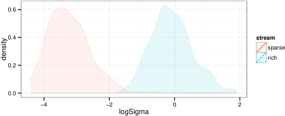
Figure 7: The large values in the distribution of posterior model discrepancy, which are of the same magnitude as the variance of observation uncertainty (units of the x-axis is as natural logaritm of their ratio, see equation 1b), suggest that model developers should refine the process description predicting the rich data stream with the basic example.

Model refinement can be justified by the magnitude of the normalized discrepancy variance. Refinement is necessary up to a detail that captures the salient patterns in the observations (Wiegand et al., 2003). Therefore, it is justified when the data is good enough to reveal more details of the processes, and when those details help the modeling purpose. With the Howland case, refinement was not necessary, because, the model discrepancy was only a small fraction of the observation uncertainty (Figure 6). With the basic example, refinement was justified, despite the cost of an additional parameter, because model discrepancy variance of the rich data stream amounted to same magnitude as the observation uncertainty (Figure 7, $e^{0}=1$). In addition, refinement can be guided by the shape of the model discrepancy. With the basic example, refinement would start to look at the slope in the modeling of the rich data stream (Figure 3).

The GP approach propagates uncertainty in observations to the uncertainty of parameters in a well-grounded manner. It is fully based on probabilistic principles, and does not invoke any external information for combining multiple criteria. It avoid the modification of uncertainty estimates with weighting different data stream (Wutzler and Carvalhais, 2014). It retains the advantage that improved resolution of sampling also leads to a more precise estimation of model parameters, given that the model is able to resolve the patterns emerging at the high resolution.

The acceptance of more parameter vectors with the GP-approach compared to the approach ignoring discrepancy is feature not a flaw. The resulting higher estimates of parameter and prediction uncertainty are more realistic, because there is less information in model-data residuals that are correlated due to model discrepancy. But how can the approach decide in which shares the model-data residuals are explained by either the mechanistical model or the statistical GP model of discrepancies? The allocation of model-data misfit, to either the mechanistical model or the statistical GP model, is solved by penalizing large model discrepancies (1cv). Parameter vectors that yield predictions with low discrepancy lead to low estimates of the signal variance and in turn to high penalties and low probabilities for other parameter vectors.

4.2 Application to larger data streams

While the GP approach worked well for the basic example, there were practical problems with application to larger problems, which were tackled by the proposed sampling scheme.

The first problem is that an inversion using rich data streams with several thousand records (Luo et al., 2011) must use many supporting points for the GP if correlation length becomes small. That leads to the construction of huge matrices that need to be inverted often. We tackled this problem by constraining the choices of supporting points and correlation length (B).

The second problem is the slow mixing of model parameters and model discrepancies when parameters and discrepancies are sampled separately (Brynjarsdóttir and O’Hagan, 2014). In this study, we tackled this problem by conditioning the model discrepancies on observed model-data residuals, i.e. treating them as latend variables, and recomputing them on each draw of new model parameters or correlation length. The posterior density of model parameters then is a part of the joint likelihood of model parameters and inferred discrepancies. This derivation resulted in an additional term per data stream in the density of model parameters that penalizes large model discrepancies (A).

The third problem is to specify appropriately spaced supporting points (triangles in figure 1) if correlation length $\psi$ is not well known a priori. If the points are spaced to close to each other, the matrices become numerically singular (Brynjarsdóttir and O’Hagan, 2014). If the points are spaced too wide, the underlying function may not be captured well. We tackled this problem by re-arranging the supporting points for each proposed correlation length. In addition, we introduced some randomness in selecting supporting points for a given correlation length. This avoided being trapped in states with lucky choices of supporting locations that yield exceptionally high likelihoods of observations.

The proposed sampling scheme tackled those problems and allowed successfull application to real world data of several thousand records.

4.3 Combination with fast optimizers

The proposed formulation (1cs - 1cv) makes it possible to combine the advantages of gradient-based optimization with GP-based representation of model discrepancy.

Speed is one advantage of gradient-based optimization compared to Bayesian sampling. The proposed Bayesian sampling scheme converges faster and is numerically less demanding than a sampling scheme that needs to sample discrepancies at the supporting locations. However, many real world problems employ models with longer run-time and cannot affort Monte-Carlo approaches, but must rely on gradient-based optimization for model calibration.

With gradient-based optimization, the parameters of the GP could not be estimated from the data any more. They had to be specified a priory based on reasonable expectations about the magnitude of the model discrepancy, i.e. signal variance, and the smoothness of the discrepancy, i.e. the correlation length. The advantages of the GP-based representation held true, despite the specification of a conservatively large signal variance for the sparse data stream with the basic example (Section 3.1.3).

A first order estimate of uncertainty in model parameters can be obtained from the curvature, i.e. Hessian matrix at the optimum of a gradient-based solution. Whenever computationally possible this estimate should be improved in a second step by a Bayesian sampling scheme. In this second step also the GP parameters can be estimated from the data as their uncertainty contributes to the uncertainty of parameters and predictions.

5 Conclusions

Based on results of different sampling scenarios of the basic model example and of the ecosystem case we conclude:

• Neglecting model discrepancies during the sampling leads to, first, underestimation of posterior uncertainty, and second, preferential allocation of model discrepancy to sparse data streams.

• Explicitly accounting for model discrepancy by representing it as a Gaussian processes (GP) successfully tackles both problems.

• The proposed sampling scheme, which treats model discrepancies as latent variable, tackles several computational problems occuring with large data streams. It allows application of the GP approach to real world inverse problems.

• The proposed formulation can combine advantages of gradient-based optimization with GP-based representation of model discrepancy.

When inverting a model using multiple data streams, it is important to explicitly account for model discrepancies. The presented GP formulation efficiently balances allocation of model discrepancy to imbalanced data streams and allows an improved inference on modelled processes.

Appendix A Sampling details

Table 2: Notation. Stream subscript $k$ is omitted for brevity.

Symbol	description
$\mathbf{o}$	observations. vector of size $n_{k}$
$\boldsymbol{\theta}$	model parameters
$\mathbf{g}(\boldsymbol{\theta})$	vector of model prediction for each observation
$\mathbf{t}$	locations of the observations, here their times. vector of size $n_{k}$
$\mathbf{z}$	model-data residuals. $\mathbf{z}=\mathbf{o}-\mathbf{g}(\boldsymbol{\theta})=\mathbf{z}_{s}\cup\mathbf{z}_{r}$
$\mathbf{z}_{s}$	model-data residuals at supporting locations $\mathbf{s}\subset\mathbf{t}$.
$\mathbf{z}_{r}$	model-data residuals at remaining locations $\mathbf{r}=\mathbf{t}\setminus\mathbf{s}$.
$\mathbf{d}$	model-process residuals. $\mathbf{d}=\mathbf{o}-\left[\mathbf{g}(\boldsymbol{\theta})+\boldsymbol{\delta}\right]$
$\psi$	correlation length of model discrepancies
$\sigma^{2}_{\epsilon}$	variance of observation uncertainty.
$\sigma^{2}_{d}$	variance of model discrepancy, i.e. signal variance of the Gaussian process (GP).
$\sigma^{2}$	normalized variance of model discrepancies. $\sigma^{2}=\sigma^{2}_{d}/\sigma^{2}_{\epsilon}$ (1b)
$\boldsymbol{\delta}$	model discrepancy. $\boldsymbol{\delta}=\boldsymbol{\delta}_{s}\cup\boldsymbol{\delta}_{r}$
$\boldsymbol{\Lambda}_{\mathbf{i},\mathbf{j}}$	Correlation matrix between two vectors of locations $\mathbf{i},\mathbf{j}\subseteq\mathbf{t}$. It depends on $\psi$
$\mathbf{K}_{\mathbf{i},\mathbf{j}}$	Covariance matrix between two vectors of model locations. $\mathbf{K}_{\mathbf{i},\mathbf{j}}=\sigma^{2}_{d}\boldsymbol{\Lambda}_{\mathbf{i},\mathbf{j}}$
$\mathbf{K}_{z}$	Covariance matrix with observation noise. $\mathbf{K}_{z}=\mathbf{K}_{\mathbf{s},\mathbf{s}}+\sigma^{2}_{\epsilon}\mathbf{I}$

The following section details the sampling of parameters for one data stream. All quantities except model parameters, $\boldsymbol{\theta}$, are stream specific. For brevity the stream index $k$ is omitted.

A complete formulation of the model is the following

$$\mathbf{o}|\boldsymbol{\theta},\boldsymbol{\delta}\sim N\left(g(\boldsymbol{\theta})+\boldsymbol{\delta},\sigma^{2}_{\epsilon}\mathbf{I}\right)$$ (1cg)

$$\left[\boldsymbol{\theta}\right]\propto 1$$ (1ch)

$$\boldsymbol{\delta}|\psi,\sigma^{2}_{d}\sim GP\left(\mathbf{0},K(\psi,\sigma^{2}_{d})\right)$$ (1ci)

$$\psi\sim\mathrm{trGamma}(a_{\psi},b_{\psi})$$ (1cj)

$$\sigma^{2}_{d}=\sigma^{2}\sigma^{2}_{\epsilon}\,,\sigma^{2}\sim\mathrm{IG}(\alpha_{\sigma^{2}},\beta_{\sigma^{2}}),$$ (1ck)

where, in the presented examples the prior for model parameters $\boldsymbol{\theta}$ was uniform, and $\mathrm{trGamma}$ denotes the truncated gamma distribution. The covariance function of the GP, here, was a squared exponential function: $K(x_{p},x_{q};\psi,\sigma^{2}_{d})=\sigma^{2}_{d}exp(-(x_{p}-x_{q})^{2}/\psi^{2}+\sigma^{2}_{\epsilon}\delta_{pq})$, where the Kronecker delta $\delta_{pg}$ equals one for $p=q$ and zero otherwise. In this study we knew that the correlation length of model discrepancies had to be of similar magnitude as the range of observation locations and used a prior to yield a mean of one third of the range of locations, $r(\mathbf{x}_{k})$, and variance of $r(\mathbf{x}_{k})^{2}/3.2$, specifically $(a_{\psi},b_{\psi})=(1.14,0.188)$ for the sparse data stream. In order to avoid numeric instability, the Metropolis step of $\psi$ rejected proposals if they fell outside the truncation bounds described in B. The prior density of the normalized discrepancy variance is an Inverse Gamma distribution. We used $\alpha_{\sigma^{2}}=1.005$ and $\beta_{\sigma^{2}}=0.1$ to yield a rather flat prior distribution with mean 20 and mode 0.5.

The Block-at-a-Time Metropolis-Hastings algorithm proceeds by several cycles with each cycle in turn sampling several blocks, i.e. subsets of the parameter vector (Hastings, 1970; Chib and Greenberg, 1995; Andrieu et al., 2003). Here we use a Metroplis sampling block for each $\psi_{k}$, another Metropolis sampling block for $\boldsymbol{\theta}$, and Gibbs sampling blocks for each $\sigma^{2}_{d,k}$. We briefly recall the Metropolis-Markov chain procedure to sample a random variable for which the probability density ist known up to a constant. At the beginning of each Metropolis sampling block a new parameter proposal is generated. In this study we generated proposals by using DEMC, which suggests steps in parameter space based on the distribution the parameter among several sampling chains (ter Braak and Vrugt, 2008). Next, model discrepancies, and the conditional probability for proposed block parameters are computed. These are also re-computed for the current block parameters if parameters that are used by the probability function have been updated by other blocks. Next a Metropolis decision accepts the proposed state if the ratio of the probabilties (proposed to current) is larger than a random number drawn from $U(0,1)$. If accepted, the proposed parameter is recorded as new sample, otherwise the current parameter is recorded again.

Correlation length $\psi$ is sampled by a Metropolis-Hastings block. The full conditional distribution of $\psi$ is

$$p\left(\psi|\mathbf{o}\right)=\frac{p\left(\psi,\hat{\boldsymbol{\delta}}|\mathbf{o}\right)}{p\left(\hat{\boldsymbol{\delta}}|\psi,\mathbf{o}\right)}\propto\frac{p(\mathbf{o}|\psi,\hat{\boldsymbol{\delta}})\,p(\psi,\hat{\boldsymbol{\delta}})}{p\left(\hat{\boldsymbol{\delta}}|\psi,\mathbf{o}\right)}=\frac{p(\mathbf{o}|\psi,\hat{\boldsymbol{\delta}})\,p(\hat{\boldsymbol{\delta}}|\psi)p(\psi)}{p\left(\hat{\boldsymbol{\delta}}|\psi,\mathbf{o}\right)}$$ (1cl)

$$p(\mathbf{o}|\psi,\hat{\boldsymbol{\delta}})\propto exp\left(-\frac{1}{2\sigma^{2}_{\epsilon}}\|\mathbf{o}-\left(\mathbf{g}+\hat{\boldsymbol{\delta}}\right)\|^{2}\right)$$ (1cm)

$$p(\psi)=p_{\Gamma}(a_{\psi},b_{\psi})\propto\psi^{a_{\psi}-1}\,e^{-b_{\psi}\psi}$$ (1cn)

$$\frac{p(\hat{\boldsymbol{\delta}}|\psi)}{p\left(\hat{\boldsymbol{\delta}}|\psi,\mathbf{o}\right)}=\frac{(2\pi)^{-n_{k}/2}|\mathbf{K}_{\boldsymbol{\delta}}|^{-1/2}e^{-\frac{1}{2}\,(\hat{\boldsymbol{\delta}}-\mathbf{0})\mathbf{K}_{\boldsymbol{\delta}}^{-1}(\hat{\boldsymbol{\delta}}-\mathbf{0})}}{(2\pi)^{-n_{k}/2}|\mathbf{K}_{\boldsymbol{\delta}}|^{-1/2}\,e^{0}}\approx e^{-\frac{1}{2}\,\hat{\boldsymbol{\delta}}_{s}\mathbf{K}_{ss}^{-1}\hat{\boldsymbol{\delta}}_{s}}$$ (1co)

$$\mathbf{K}_{\boldsymbol{\delta}}=\left[\mathbf{K}_{ss},\mathbf{K}_{sr};\mathbf{K}_{rs},\mathbf{K}_{rr}\right],$$ (1cp)

where the depencies on $\boldsymbol{\theta}$ and $\sigma^{2}_{d}$ and the stream index, $k$, are omitted for brevity. The first step in (1cl) derives from a factorization of the joint density of $\psi$ and $\hat{\boldsymbol{\delta}}$. The second step is the Bayes rule. The third step is the factorization of the joint unconditional density of $\hat{\boldsymbol{\delta}}$ and $\psi$.

The Likelihood 1cl is based only on the expected value of model discrepancy and does not require a sample of model discrepancy. It actually holds for any particular sample of model discrepancy $\boldsymbol{\delta}$, but choosing the expected value $\hat{\boldsymbol{\delta}}$ greatly simplifies calculations (1co). The normalizing factor in (1co) cancels. The numerator is the probability density of $\hat{\boldsymbol{\delta}}$ without knowning the observations, i.e. a multivariate normal density of the GP with zero mean. The denominator is the probability conditioned on the current observations and predictions, i.e. a multivariate normal density with mean $\hat{\boldsymbol{\delta}}$. The inversion of the blocked matrix $\mathbf{K}_{\boldsymbol{\delta}}$ could be done using blockwise inversion. However, it still requires an inversion of a matrix of dimension of the number of non-supporting locations $r$, and has the danger of becoming numerically singular. We suggest approximating the norm by only using the supporting locations. Due to the relation between spacing of supporting locations and the correlation length (B), the approximation stayed within one per mill precision in our applications so far. The relation also prevents $\mathbf{K}_{\mathbf{s},\mathbf{s}}$ from becoming numerically singular. If $\mathbf{K}_{\mathbf{s},\mathbf{s}}$ became numerically singular, a small diagonal component could be added.

The vector of expected value of model discrepancies $\hat{\boldsymbol{\delta}}=\hat{\boldsymbol{\delta}}_{s}\cup\hat{\boldsymbol{\delta}}_{r}$ is computed as function of parameters $\boldsymbol{\theta}$, $\psi$, and $\sigma^{2}_{d}$ based on the model model-data residuals at supporting locations, $\mathbf{z}_{s}$ (Rasmussen and Williams, 2006)

$$\hat{\boldsymbol{\delta}_{s}}=\mathbf{K}_{\mathbf{s},\mathbf{s}}\mathbf{K}_{z}^{-1}\mathbf{z}_{s}$$ (1cq)

$$\hat{\boldsymbol{\delta}_{r}}=\mathbf{K}_{\mathbf{r},\mathbf{s}}\mathbf{K}_{\mathbf{s},\mathbf{s}}^{-1}\boldsymbol{\delta}_{s}=\mathbf{K}_{\mathbf{r},\mathbf{s}}\mathbf{K}_{z}^{-1}\mathbf{z}_{s}$$ (1cr)

Note that covariance matrices $\mathbf{K}$ depend on current discrepancy variance $\sigma_{d}^{2}$ and correlation length $\psi$, and that $\mathbf{z}_{s}$ depends on parameters $\boldsymbol{\theta}$ and observations $\mathbf{o}$.

Model parameters $\boldsymbol{\theta}$ are sampled by Metropolis-Hastings block. Their conditional distribution depends on all data streams, $k$. We assume that observations and model discrepancies are independent between different streams.

$$p\left(\boldsymbol{\theta}|\mathbf{o}\right) =\frac{p\left(\boldsymbol{\theta},\hat{\boldsymbol{\delta}}|\mathbf{o}\right)}{p\left(\hat{\boldsymbol{\delta}}|\boldsymbol{\theta},\mathbf{o}\right)}\propto\frac{p(\mathbf{o}|\boldsymbol{\theta},\hat{\boldsymbol{\delta}})\,p(\hat{\boldsymbol{\delta}}|\boldsymbol{\theta})\,p(\boldsymbol{\theta})}{p\left(\hat{\boldsymbol{\delta}}|\boldsymbol{\theta},\mathbf{o}\right)}$$ (1cs)

$$=\prod_{k}p(\mathbf{o}_{k}|\boldsymbol{\theta},\hat{\boldsymbol{\delta}}_{k})\,\frac{p(\hat{\boldsymbol{\delta}}_{k}|\boldsymbol{\theta})}{p\left(\hat{\boldsymbol{\delta}}_{k}|\boldsymbol{\theta},\mathbf{o}_{k}\right)}\,p(\boldsymbol{\theta})$$ (1ct)

$$p(\boldsymbol{\theta}) \propto 1$$ (1cu)

$$\frac{p(\hat{\boldsymbol{\delta}}_{k}|\boldsymbol{\theta})}{p\left(\hat{\boldsymbol{\delta}}_{k}|\boldsymbol{\theta},\mathbf{o}_{k}\right)} =exp(-1/2\,\hat{\boldsymbol{\delta}}_{k}\mathbf{K}_{\boldsymbol{\delta},k}^{-1}\hat{\boldsymbol{\delta}}_{k})\approx exp(-1/2\,\hat{\boldsymbol{\delta}}_{s,k}\mathbf{K}_{ss,k}^{-1}\hat{\boldsymbol{\delta}}_{s,k}),$$ (1cv)

where, the dependence on all hyperparameters $\psi_{k}$ and $\sigma^{2}_{d,k}$ has been omitted for brevity. The derivation of each stream-factor is analogous to the derivation of conditional density $p\left(\psi|\mathbf{o}\right)$ above, unless the simplification that the normalizing factor of $p(\hat{\boldsymbol{\delta}}_{k})$ does not depend on $\boldsymbol{\theta}$. Note that a penalty term (1cv) for each stream model discrepancy must be included in the conditional density function of the parameter vector. Again, we approximated the norm of the vector of all model discrepancies $\hat{\boldsymbol{\delta}}_{k}$ by the norm of the model discrepancies at supporting locations $\hat{\boldsymbol{\delta}}_{s,k}$.

Normalized discrepancy variance $\sigma^{2}$ was sampled from an inverse Gamma distribution conditioned on discrepancies derived for current parameters.

$$\sigma^{2}|\mathbf{o},\boldsymbol{\theta},\psi\sim IG\left(\alpha_{\sigma^{2}}+\frac{n_{s}}{2},\beta_{\sigma^{2}}+\frac{1}{2\sigma^{2}_{\epsilon}}||\hat{\boldsymbol{\delta}}_{s}(\mathbf{o},\boldsymbol{\theta},\psi,\sigma^{2}_{d})||_{\Lambda_{ss}^{-1}}\right),$$ (1cw)

where $n_{s}$ is the number of supporting locations and $\alpha_{\sigma^{2}}$, $\beta_{\sigma^{2}}$ are parameters of the prior probability density. The factor $1/\sigma^{2}_{\epsilon}$ needs to be included, because we specified the prior for the discrepancy variance normalized by variance of observation uncertainties. We did not encounter problems when reusing the current value of $\sigma^{2}_{d}$ in the calculation of discrepancy. However, one could instead use a data-based discrepancy variance to prevent this dependence and potential feedback behaviour. A data-based estimate can be found by maximising the likelihood of observed residuals given all the other parameters and observation uncertainty.

Appendix B Limits for choosing supporting points $\mathbf{s}$ and truncation of sampling correlation length $\psi$

For large correlation length $\psi$, some matrices used in the calculation of model discrepancies $\delta_{s}$ become numerically singular. Further, different correlation length that are larger than the range of the data, $t$, cannot be distinguished. Hence, an upper bound of $(max(t)-min(t))$ is applied to the sampling of $\psi$.

For very small correlation length, model discrepancy goes to the expected value zero between supporting points. However, we want to model a smooth discrepancy between supporting points. Hence, a lower bound of 2/3 of the mean distance between supporting points is applied to the sampling of $\psi$.

Supporting points are chosen among observation points closest to a grid with distance $3\psi/2$, with a minimal spacing so that there are two points between supporting points and a maximal spacing so that there are at least five supporting points.

Appendix C Dalec-Howland inversion additional results

Eight chains from two independent populations converged to the same limiting distribution (Figure 8).

Figure 8: Trace and marginal distribution of the tails of eight Chains from two independent populations sampling 15 parameters of the DALEC model. They indicate good mixing and convergence to the limiting distribution.

The variance of the marginals of posterior probability density inferred by the GP approach, was intermediate between the ignore and the blocked inversion scenarios. The location of the mode was mostly in between the two other approaches (Figure 9).

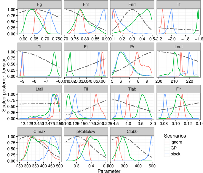
Figure 9: Marginals of posterior probability density of inverting the DALEC model. The thick dash-dot line represents prior parameter density.

Prediction during calibration period are quite similar across inversion scenarios (Figure 10). Nevertheless there were differences in uncertainty of posterior predictions (Figure 5).

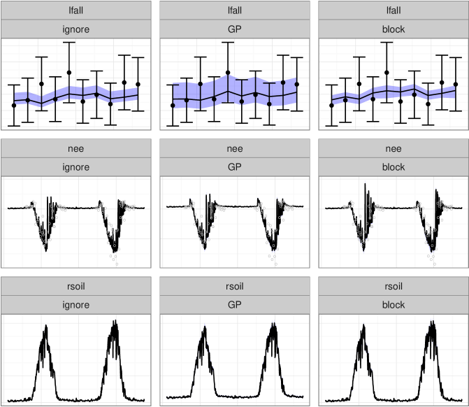
Figure 10: Comparsion of model predictions to observations of the DALEC inversion during the calibration period. Columns represent different inversion scenarios. ignore: ignoring model discrepancies, GP: Gaussian processes approach, blocks: parameter block approach. Rows show different data streams. Litterfall is shown for predictions of 10 years of calibration period. NEE and respiration are shown for the last two of the 10 years.

References

- (1)
- Ahrens et al. (2014) Ahrens, B., Reichstein, M., Borken, W., Muhr, J., Trumbore, S. E. and Wutzler, T. (2014). Bayesian calibration of a soil organic carbon model using delta-14c measurements of soil organic carbon and heterotrophic respiration as joint constraints, Biogeosciences 11(8): 2147–168.
- Andrieu et al. (2003) Andrieu, C., De Freitas, N., Doucet, A. and Jordan, M. I. (2003). An introduction to mcmc for machine learning, Machine learning 50(1-2): 5–43.
- Bormann et al. (2003) Bormann, N., Saarinen, S., Kelly, G. and Thépaut, J.-N. (2003). The spatial structure of observation errors in atmospheric motion vectors from geostationary satellite data, Monthly Weather Review 131(4): 706–718.
- Brynjarsdóttir and O’Hagan (2014) Brynjarsdóttir, J. and O’Hagan, A. (2014). Learning about physical parameters: the importance of model discrepancy, Inverse Problems 30(11): 114007.
- Chib and Greenberg (1995) Chib, S. and Greenberg, E. (1995). Understanding the Metropolis-Hastings algorithm, American Statistician 49: 327–335.
- Desroziers et al. (2005) Desroziers, G., Berre, L., Chapnik, B. and Poli, P. (2005). Diagnosis of observation, background and analysis-error statistics in observation space, Q. J. R. Meteorol. Soc. 131(613): 3385–3396.
- Gelman et al. (2003) Gelman, A., Carlin, J., Stern, H. and Rubin, D. (2003). Bayesian Data Analysis. 2003, Boca Raton (FL): Chapman Hall .
- Hastings (1970) Hastings, W. (1970). Monte carlo sampling methods using markov chains and their applications, Biometrika 57(1): 97–109.
- Healy and White (2005) Healy, S. and White, A. (2005). Use of discrete Fourier transforms in the 1D-var retrieval problem, Q. J. R. Meteorol. Soc. 131(605): 63–72. neglecting correlations leads to overestimation of information content.
- Hollinger et al. (2004) Hollinger, D. Y., Aber, J., Dail, B., Davidson, E. A., Goltz, S. M., Hughes, H., Leclerc, M. Y., Lee, J. T., Richardson, A. D., Rodrigues, C. and et al. (2004). Spatial and temporal variability in forest-atmosphere CO2 exchange, Global Change Biology 10(10): 1689–1706.
- Hollinger and Richardson (2005) Hollinger, D. Y. and Richardson, A. D. (2005). Uncertainty in eddy covariance measurements and its application to physiological models, Tree Physiology 25(7): 873–885.
- Keenan et al. (2011) Keenan, T. F., Carbone, M. S., Reichstein, M. and Richardson, A. D. (2011). The model–data fusion pitfall: assuming certainty in an uncertain world, Oecologia 167(3): 587–597.
- Kennedy and O’Hagan (2001) Kennedy, M. C. and O’Hagan, A. (2001). Bayesian calibration of computer models, Journal of the Royal Statistical Society. Series B, Statistical Methodology pp. 425–464.
- Luo et al. (2011) Luo, Y., Ogle, K., Tucker, C., Fei, S., Gao, C., LaDeau, S., Clark, J. S. and Schimel, D. S. (2011). Ecological forecasting and data assimilation in a data-rich era, Ecological Applications 21(5): 1429–1442.
- Metropolis et al. (1953) Metropolis, N., Rosenbluth, A. W., Rosenbluth, M. N., Teller, A. H. and Teller, E. (1953). Equation of state calculations by fast computing machines, The journal of chemical physics 21(6): 1087–1092.
-
Miettinen (1999)
Miettinen, K. (1999).
Nonlinear multiobjective optimization, volume 12 of international
series in operations research and management science.
http://users.jyu.fi/~miettine/book/ - Nash (1990) Nash, J. C. (1990). Compact numerical methods for computers: linear algebra and function minimisation, CRC Press.
-
R Core Team (2016)
R Core Team (2016).
R: A Language and Environment for Statistical Computing, R
Foundation for Statistical Computing, Vienna, Austria.
https://www.R-project.org -
Rasmussen and Williams (2006)
Rasmussen, C. E. and Williams, C. K. I. (2006).
Gaussian Processes for Machine Learning, The MIT Press.
http://www.gaussianprocess.org/gpml/chapters/ - Reich and Cotter (2015) Reich, S. and Cotter, C. (2015). Probabilistic Forecasting and Bayesian Data Assimilation, Cambridge University Press.
- Richardson et al. (2010) Richardson, A., Williams, M., Hollinger, D., Moore, D., Dail, D., Davidson, E., Scott, N., Evans, R., Hughes, H., Lee, J., Rodrigues, C. and Savage, K. (2010). Estimating parameters of a forest ecosystem c model with measurements of stocks and fluxes as joint constraints, Oecologia pp. –.
- Tarantola (2005) Tarantola, A. (2005). Inverse Problems Theory, Methods for Data Fitting and Model Parameter Estimation, SIAM, Philadelphia.
- ter Braak and Vrugt (2008) ter Braak, C. and Vrugt, J. (2008). Differential Evolution Markov Chain with snooker updater and fewer chains, Statistics and Computing 18(4): 435–446.
- Waller et al. (2014) Waller, J. A., Dance, S. L., Lawless, A. S. and Nichols, N. K. (2014). Estimating correlated observation error statistics using an ensemble transform Kalman filter, Tellus A 66(0). estimation of error covariance matrix by DBCP diagnostics, here slowly varying with time.
- Weston et al. (2014) Weston, P. P., Bell, W. and Eyre, J. R. (2014). Accounting for correlated error in the assimilation of high-resolution sounder data, Q.J.R. Meteorol. Soc. 140(685): 2420–2429.
- Wiegand et al. (2003) Wiegand, T., Jeltsch, F., Hanski, I. and Grimm, V. (2003). Using pattern-oriented modeling for revealing hidden information: a key for reconciling ecological theory and application, Oikos 100(2): 209–222.
- Williams et al. (2005) Williams, M., Schwarz, P. A., Law, B. E., Irvine, J. and Kurpius, M. R. (2005). An improved analysis of forest carbon dynamics using data assimilation, Global Change Biology 11(1): 89–105.
- Wutzler and Carvalhais (2014) Wutzler, T. and Carvalhais, N. (2014). Balancing multiple constraints in model-data integration: Weights and the parameter-block approach, J. Geophys. Res. Biogeosci. 119(11): 2112–2129.
- Zobitz et al. (2011) Zobitz, J., Desai, A., Moore, D. and Chadwick, M. (2011). A primer for data assimilation with ecological models using markov chain monte carlo (mcmc), Oecologia 167(3): 599–611.