Experimental Low-Latency Device-Independent Quantum Randomness

Abstract

Applications of randomness such as private key generation and public randomness beacons require small blocks of certified random bits on demand. Device-independent quantum random number generators can produce such random bits, but existing quantum-proof protocols and loophole-free implementations suffer from high latency, requiring many hours to produce any random bits. We demonstrate device-independent quantum randomness generation from a loophole-free Bell test with a more efficient quantum-proof protocol, obtaining multiple blocks of $512$ random bits with an average experiment time of less than $5\;\mathrm{min}$ per block and with a certified error bounded by $2^{-64}\approx 5.42\times 10^{-20}$.

A fundamental feature of quantum mechanics is that measurements of a quantum system can have random outcomes even when the system is in a definite, pure state. By definition, pure states are completely uncorrelated with every other physical system, which implies that the measurement outcomes are intrinsically unpredictable by anyone outside the measured quantum system’s laboratory. The unpredictability of quantum measurements is exploited by conventional quantum random number generators (QRNGs) Herrero-Collantes and Garcia-Escartin (2017) for obtaining random bits whose distribution is ideally uniform and independent of other systems. The use of such QRNGs requires trust in the underlying quantum devices Pironio and Massar (2013). A higher level of security is attained by device-independent quantum random number generators (DIQRNGs) Colbeck (2006); Colbeck and Kent (2011) based on loophole-free Bell tests, where the randomness produced can be certified even with untrusted quantum devices that may have been manufactured by dishonest parties. The security of a DIQRNG relies on the physical security of the laboratory to prevent unwanted information leakage, and on the trust in the classical systems that record and process the outputs of quantum devices for randomness generation.

Since the idea of DIQRNGs was introduced in Colbeck’s thesis Colbeck (2006), many DIQRNG protocols have been developed—for a review see Acín and Masanes (2016). These protocols generally exploit quantum non-locality to certify entropy but differ in device requirements, Bell-test configurations, randomness rates, finite-data efficiencies, and the security levels achieved. We can classify protocols by whether they are secure in the presence of classical or quantum side information, in other words, by whether they are classical- or quantum-proof.

The first experimentally accessible DIQRNG protocol was given and implemented by Pironio et al. Pironio et al. (2010) with a detection-loophole-free Bell test using entangled ions. They certified $42$ bits of classical-proof entropy with error bounded by $0.01$, where, informally, the error can be thought of as the probability that the protocol output does not satisfy the certified claim. This required about one month of experiment time. To improve this result required the advent of loophole-free Bell tests and much more efficient protocols. Such a protocol and experimental implementation with an optical loophole-free Bell test was given by Bierhorst et al. Bierhorst et al. (2018) and obtained $1024$ classical-proof random bits with error $10^{-12}$ in $10\;\mathrm{min}$. There have been three demonstrations of quantum-proof DIQRNGs, all with photons. The first two were subject to the locality and freedom-of-choice loopholes Bell (2004). They obtained $4.6\times 10^{7}$ random bits with error $10^{-5}$ in $111\;\mathrm{h}$ Liu et al. (2018a), and $6.2\times 10^{5}$ random bits with error $10^{-10}$ in $43\;\mathrm{min}$ Shen et al. (2018), respectively. The third was loophole-free and obtained $6.2\times 10^{7}$ random bits with error $10^{-5}$ in $96\;\mathrm{h}$ Liu et al. (2018b).

The quantum-proof experiments described above aimed for good asymptotic rates. To approach the asymptotic rate requires a very large number of trials to certify a large amount of entropy. However, many if not most applications of certified randomness require only short blocks of fresh randomness. To address these applications, we consider instead a standardized request for $512$ random bits with error $2^{-64}\approx 5.42\times 10^{-20}$ and with minimum delay, or latency, between the request and delivery of bits satisfying the request. In this work, we consider only the contribution of experiment time to latency. The previous quantum-proof DIQRNG implemented with a loophole-free Bell test Liu et al. (2018b) would have required at least $24.1\;\mathrm{h}$ to satisfy the standardized request—see Sect. V of the Supplemental Material (SM).

In this letter, we reduce the latency required to produce $512$ device-independent and quantum-proof random bits with error $2^{-64}$ by orders of magnitude. For this purpose, here we implement a quantum-proof protocol developed in the companion paper (CP) Zhang et al. (2018a) with a loophole-free Bell test. Unlike other demonstrations of quantum-proof DIQRNGs, we conservatively account for adversarial bias in the setting choices, and we show repeated fulfillment of the standardized request. We obtain five successive blocks of $512$ random bits with error $2^{-64}$ and with an average experiment time of less than $5\;\mathrm{min}$ per block.

Overview of theory. We give a high-level description of the features of our protocol. For formal definitions and technical details, see the CP Zhang et al. (2018a). Our protocol is based on repeated (but not necessarily independent or identical) trials of a loophole-free CHSH Bell test Clauser et al. (1969), consisting of a source $\mathsf{S}$ and two measurement stations $\mathsf{A}$ and $\mathsf{B}$ (see Fig. 2). In each trial, the source attempts to distribute a pair of entangled photons to the stations, the protocol randomly chooses binary measurement settings $X$ and $Y$ for the stations, the corresponding measurements are performed, and the binary outcomes $A$ and $B$ are recorded. We call $Z=XY$ and $C=AB$ the input and output of the trial, respectively.

An end-to-end randomness generation protocol starts with a request for $k$ random bits with error $\epsilon$. The user then chooses a positive quantity $\sigma$ (the entropy threshold for success) and positive errors $\epsilon_{\sigma},\epsilon_{x}$ (the entropy error and the extractor error, respectively) whose sum is no more than $\epsilon$. The quantity $\sigma$ chosen by the user must satisfy the inequality $\sigma\geq k+4\log_{2}(k)+4\log_{2}(2/\epsilon_{x}^{2})+6$. This inequality is sufficient to guarantee that, if the outputs of the experiment can be proven to have entropy at least $\sigma$, then $k$ random bits can be extracted. (The randomness extractor that we use for this purpose is Trevisan’s extractor Trevisan (2001) as implemented by Mauerer, Portmann and Scholz Mauerer et al. (2012). We refer to it as the TMPS extractor—see Sect. II of the SM.) The user also needs to decide the maximum number $n$ of Bell-test trials to run. For simplicity, we temporarily assume that a fixed number $n$ of trials will be executed, but in the implementation as described in a later section we exploit the ability to stop early.

After fixing the parameters defined in the previous paragraph, $n$ Bell-test trials are sequentially executed, and the inputs and outputs are recorded as $\mathbf{Z}=(Z_{i})_{i=1}^{n}$ and $\mathbf{C}=(C_{i})_{i=1}^{n}$, where $Z_{i}$ and $C_{i}$ are the input and output of the $i$’th trial. The upper-case symbols $\mathbf{C}$, $C_{i}$, $\mathbf{Z}$ and $Z_{i}$ are treated as random variables, and their values are denoted by the corresponding lower-case symbols. Let $\mathsf{E}$ denote the “environment” of the experiment, including any quantum side information that could be possessed by an adversary. The entropy of the outputs $\mathbf{C}$ is quantified by the quantum $\epsilon_{\sigma}$-smooth conditional min-entropy of $\mathbf{C}$ given $\mathbf{Z}\mathsf{E}$ Renner (2006). We refer to this quantity as the output entropy. The user can estimate the output entropy as described in the next section and check whether that estimate is at least $\sigma$. If not, the protocol fails and a binary variable $P$ is set to $P=0$; otherwise, the protocol succeeds and $P=1$.

When the protocol succeeds, we apply the TMPS extractor Mauerer et al. (2012) to extract $k$ random bits with error $\epsilon$. The TMPS extractor is a classical algorithm that is applied to the outputs $\mathbf{C}$ as well as a random seed $S$, and produces a bit string $R$. The final state of the protocol then consists of the classical variables $RS\mathbf{Z}P$ and the quantum system $\mathsf{E}$. In the CP Zhang et al. (2018a), we prove that the protocol is $\epsilon$-sound in the following sense: The error $\epsilon$ is an upper bound on the product of the success probability and the purified distance Tomamichel (2016) between the actual state of $RS\mathbf{Z}\mathsf{E}$ conditional on the success event $P=1$ and an ideal state of $RS\mathbf{Z}\mathsf{E}$, according to which $RS$ is uniformly random and independent of $\mathbf{Z}\mathsf{E}$. For the protocol to be useful, it is necessary that the probability of success in the actual implementation can be close to $1$, a property referred to as completeness. With properly configured quantum devices, it is possible to make this probability exponentially close to $1$ by increasing the number of trials executed. Soundness and completeness imply formal security of the protocol.

Estimating entropy. In the CP Zhang et al. (2018a), we develop the approach of certifying entropy by “quantum estimation factors” (QEFs), a general technique that generalizes previous certification techniques against quantum side information Miller and Shi (2017); Arnon-Friedman et al. (2018). The construction of QEFs requires first defining a notion of models. The “model” for an experiment is the set of all possible final states that can occur at the end of the experiment. A final state can be written as $\rho_{\mathbf{CZ}\mathsf{E}}=\sum_{\mathbf{cz}}\ket{\mathbf{cz}}\bra{\mathbf{cz}}\otimes\rho_{\mathsf{E}}(\mathbf{cz})$, where $\rho_{\mathsf{E}}(\mathbf{cz})$ is the unnormalized state of $\mathsf{E}$ given results $\mathbf{cz}$.

Given the state $\rho_{\mathbf{CZ}\mathsf{E}}$, we characterize the unpredictability of the outputs $\mathbf{c}$ given the system $\mathsf{E}$ and the inputs $\mathbf{z}$ by the sandwiched Rényi power, denoted by $\mathcal{R}_{1+\beta}\big{(}\rho_{\mathsf{E}}(\mathbf{cz})\big{|}\rho_{\mathsf{E}}(\mathbf{z})\big{)}$ where $\beta>0$ and $\rho_{\mathsf{E}}(\mathbf{z})=\sum_{\mathbf{c}}\rho_{\mathsf{E}}(\mathbf{cz})$ (see Eq. (S2) of the SM for the explicit expression). A QEF with a positive power $\beta$ for a sequence of $n$ trials is a non-negative function $T$ of random variables $\mathbf{CZ}$ such that for all states $\rho_{\mathbf{CZ}\mathsf{E}}$ in the model, $T$ satisfies the inequality

$$\sum_{\mathbf{cz}}T(\mathbf{cz})\mathcal{R}_{1+\beta}\left(\rho_{\mathsf{E}}(\mathbf{cz})\middle|\rho_{\mathsf{E}}(\mathbf{z})\right)\leq 1.$$

Informally, one main result in the CP Zhang et al. (2018a) is that if at the conclusion of the experiment the variable $\log_{2}(T)/\beta$ takes a value at least $h$ for some $h>0$, then the output entropy (in bits) must be at least $h-\log_{2}(2/\epsilon_{\sigma}^{2})/\beta$ no matter which particular state in the model describes the experiment. Hence, for estimating entropy it suffices to construct QEFs.

In practice, the model for a sequence of trials is constructed as a chain of models for each individual trial. QEFs then satisfy a chaining property: If $F_{i}(C_{i}Z_{i})$ is a QEF with power $\beta$ for the $i$’th trial, then the product $\prod_{i=1}^{n}F_{i}(C_{i}Z_{i})$ is a QEF with power $\beta$ for the sequence of $n$ trials. To construct the QEF $T(\mathbf{CZ})$, we use this property. Moreover, since the model for each trial of our experiment is identical, we always take the same QEF for each executed trial. The CP Zhang et al. (2018a) contains general techniques for constructing models and QEFs, and the SM contains the details of constructing models (Sect. I) and QEFs (Sect. IV) for each trial of our experiment.

Experiment. Our setup is similar to those reported in Refs. Shalm et al. (2015); Bierhorst et al. (2018). A pair of polarization-entangled photons are generated through the process of spontaneous parametric downconversion and then distributed via optical fiber to Alice and Bob (see Fig. 1). At each lab of Alice and Bob, a fast QRNG with parity-bit randomness extraction Abellán et al. (2015) is used to randomly switch a Pockels cell-based polarization analyzer (see Fig. 2). Alice’s polarization measurement angles, relative to a vertical polarizer, are $a=−4.1^{\circ}$ and $a^{\prime}=25.5^{\circ}$, and Bob’s are $b=-a$ and $b^{\prime}=-a^{\prime}$. These measurement angles, along with the non-maximally entangled state prepared in Fig. 1, are chosen based on numerical simulations of our setup to achieve an optimal Bell violation. The photons are then detected in each lab using superconducting nanowire single-photon detectors with efficiency greater than $90\%$ Marsili et al. (2013). The total system efficiencies for Alice and Bob are $76.2\pm 0.3\%$ and $75.8\pm 0.3\%$, allowing the detection loophole to be closed. With the configuration detailed in Fig. 2, we can also close the locality loophole.

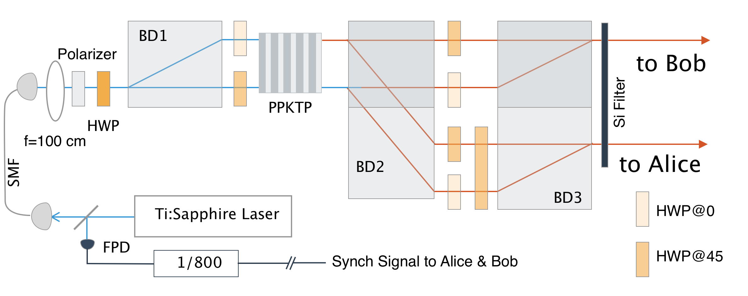
Figure 1: Diagram of the entangled photon-pair source. A $775$-nm-wavelength picosecond Ti:Sapphire laser operating at a $79.3\;\mathrm{MHz}$ repetition rate pumps a $20$-mm-long periodically-poled potassium titanyl phosphate (PPKTP) crystal, to produce degenerate photons at $1550\;\mathrm{nm}$ with a per-pulse probability of $0.0045$. The pump is transmitted through a polarization-maintaining single-mode fiber (SMF). The PPKTP crystal is cut for type-II phasematching and placed in a polarization-based Mach-Zehnder interferometer constructed using half-wave plates (HWPs) and three beam displacers (BD1, BD2 and BD3). Tuning the polarization of the pump by a polarizer and HWP allows us to create the non-maximally entangled state $\ket{\psi}=0.967\ket{HH}+0.254\ket{VV}$, where $H$ and $V$ denote the horizontally and vertically polarized single-photon states. The photons, along with a synchronization signal, are then distributed via optical fiber to Alice and Bob. The synchronization signal is generated by a fast photodiode (FPD) and divider circuit which divides the pump frequency by $800$, and is used as a clock to determine the start of a trial and to time the operation of Alice’s and Bob’s measurements. This leads to a trial rate of approximately $100\;\mathrm{kHz}$.

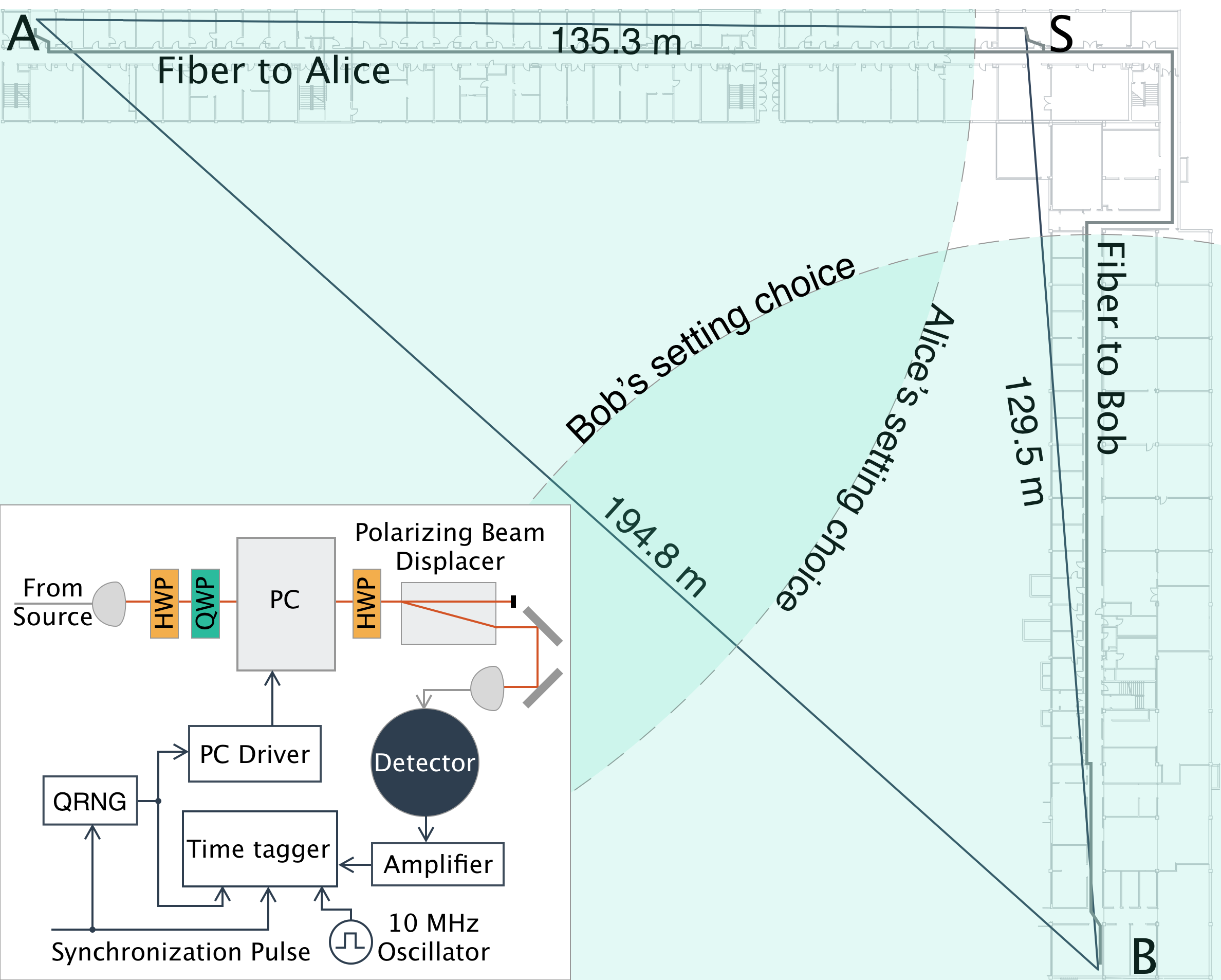
Figure 2: Locations of Alice ($\mathsf{A}$), Bob ($\mathsf{B}$), and the source ($\mathsf{S}$). Alice and Bob are separated by $194.8\pm 1.0\;\mathrm{m}$ (this is slightly further than in Refs. Shalm et al. (2015); Bierhorst et al. (2018)). Faint grey lines indicate the paths that the entangled photons take from the source to Alice and Bob through fiber optic cables. The light-green quarter circles are the 2D projections of the expanding light spheres containing the earliest available information about the random bits used for Alice’s and Bob’s setting choices at the trial. When Bob finishes his measurement, the radius of the light sphere corresponding to the start of Alice’s QRNG has expanded to $127.3\pm 0.5\;\mathrm{m}$, after which it takes an additional $222.3\pm 3.8\;\mathrm{ns}$ before the light sphere will intersect Bob’s location. Similarly, when Alice completes her measurement, the light sphere corresponding to the start of Bob’s QRNG has only reached a radius of $98.3\pm 0.5\;\mathrm{m}$, and it will take $315.5\pm 3.8\;\mathrm{ns}$ more to arrive at Alice’s station. In this way, the actions of Alice and Bob are spacelike separated. Inset: Alice’s and Bob’s measurement apparatuses both consist of a Pockels cell (PC), operating at approximately 100 KHz, and a polarizer, constructed using two have-wave plates (HWPs), a quarter-wave plate (QWP) and a polarizing beam displacer, in order to make fast polarization measurements on their respective photons. The measurement setting is controlled by a QRNG, the photon is detected by a high-efficiency superconducting nanowire single-photon detector, and the resulting signal is recorded on a time tagger, where a $10\;\mathrm{MHz}$ oscillator is used to keep Alice’s and Bob’s time taggers synchronized.

In each trial, Alice’s and Bob’s setting choices $X$ and $Y$ are made with random bits whose deviation from uniform is assumed to be bounded. That is, knowing all events in the past light cone, one should not be able to predict the next choice with a probability better than $0.5+\epsilon_{b}$. We call $\epsilon_{b}$ the (maximum) adversarial bias. In particular, it is assumed that the quantum devices used cannot have more prior knowledge of the random setting choices than the adversarial bias for each trial. Specifically, we assume that the adversarial and trial-dependent bias of Alice’s and Bob’s QRNGs is bounded by $\epsilon_{b}\leq 1\times 10^{-3}$. That is, each of the setting choices $X$ and $Y$ has a two-outcome distribution with probabilities in the interval $[0.5-1\times 10^{-3},0.5+1\times 10^{-3}]$. The bias assumption is supported in two ways: first by a quantum statistical model of the QRNGs, validated by measurements of the QRNG internal operation Abellán et al. (2015), and second by the observation that the frequencies of the output bits of each QRNG deviate from 0.5 by less than $6\times 10^{-5}$ on average in a run of $21\;\mathrm{min}$ of trials.

Protocol implementation. The goal is to obtain $k=512$ random bits with error $\epsilon=2^{-64}$. For this, we set $\epsilon_{\sigma}=0.8\times 2^{-64}$ and $\epsilon_{x}=0.2\times 2^{-64}$. To extract $k=512$ random bits with the TMPS extractor, it suffices to set the entropy threshold to be $\sigma=1089$. The implementation stages for each instance of the protocol are summarized in Box 1, and more details are available in Sect. III of the SM.

1. Calibration

   1. Determine the QEF $F(CZ)$ and its power $\beta$ used for each executed trial.

   2. Fix $n$—the maximum number of trials.

2. Randomness Accumulation: Run the experiment to acquire up to $n$ trials. After each trial $i$,

   1. Update the running $\log_{2}$-QEF value $L_{i}=\sum_{j=1}^{i}\log_{2}(F(c_{j}z_{j}))$, where $c_{j}$ and $z_{j}$ are the observed values of $C_{j}$ and $Z_{j}$.

   2. If $\big{(}L_{i}-\log_{2}(2/\epsilon_{\sigma}^{2})\big{)}/\beta\geq\sigma$, stop the experiment, set the number of trials actually executed as $n_{\text{act}}=i$, and set the success event $P=1$.

3. Randomness Extraction: If $P=1$, then extract $k$ random bits with error $\epsilon$.

Box 1 Overview of protocol implementation

Results. Ideally, the protocol would be applied concurrently with the acquisition of the experimental trials. In this case, the trials were performed three months before the protocol was fully implemented. About $89\;\mathrm{min}$ of experimental results were recorded. The results were stored in $1\;\mathrm{min}$ blocks containing approximately $6\times 10^{6}$ trials each. The first $21\;\mathrm{min}$ were unblinded for testing the protocol, and the rest were kept in blind storage until the protocol was fully implemented and ready to be used.

From the first $21\;\mathrm{min}$ of unblinded results we decided to run five sequential instances of the protocol, and for calibration in each instance we determined to use the $10\;\mathrm{min}$ of results preceding to the first trial to be used for randomness accumulation (see Sect. III of the SM for details). We note that the trials for randomness accumulation in one instance can be used also for calibration in the next instance. For the protocol, we loaded the data and divided each $1\;\mathrm{min}$ block into $60$ subblocks of approximately $1\times 10^{5}$ trials each. The protocol was then designed to use integer multiples of these subblocks. The first instance of the protocol started producing randomness at the $22$nd $1\;\mathrm{min}$ block. Each instance started at the first not-yet-used subblock and used the previous $600$ subblocks for calibration, then processed subblocks until the running entropy estimate surpassed the threshold $\sigma$. In each instance, this happened well before the maximum number of trials $n$ determined at the calibration stage was reached, leading to success of the instance. We then applied the extractor to produce $512$ random bits with error $2^{-64}$.

Table 1: Characteristics of the five protocol instances. The number of subblocks is approximately the number of seconds of experiment time required. The entropy rate is estimated by $L_{n_{\mathrm{act}}}/(\beta n_{\mathrm{act}})$, where $n_{\mathrm{act}}$ is the actual number of trials executed in an instance, $L_{n_{\mathrm{act}}}$ is the running $\log_{2}$-QEF value at the end of an instance, and $\beta$ is the power associated with the QEF which is used for each executed trial and determined at the calibration stage. The trial rate in the experiment was approximately $100\;\mathrm{kHz}$.

Instance	$n/10^{7}$	$n_{\mathrm{act}}/10^{7}$	Number	$\beta$	Entropy
			of sub-		rate$/10^{-4}$
			blocks
1	$5.25$	$2.32$	$233$	0.010	$6.07$
2	$4.74$	$3.76$	$379$	0.010	$3.78$
3	$5.92$	$2.85$	$287$	0.009	$5.47$
4	$6.20$	$2.83$	$285$	0.009	$5.53$
5	$5.49$	$2.72$	$274$	0.010	$5.20$

The results are summarized in Tab. 1. It shows that the experiment time required to fulfill the request for $512$ quantum-proof random bits with error $2^{-64}$ is less than $5\;\mathrm{min}$ on average, demonstrating a dramatic improvement over other quantum-proof protocols and previous experiments. The only experimentally accessible alternative quantum-proof protocol is entropy accumulation as described in Ref. Arnon-Friedman et al. (2018). We found that satisfying the request using theoretical results from Ref. Arnon-Friedman et al. (2018), with our experimental configuration and performance, would have required at least $6.108\times 10^{10}$ trials, corresponding to $169.7\;\mathrm{h}$ of experiment time—see Sect. V of the SM for details.

In conclusion, we demonstrated five sequential instances of the DIQRNG protocol. For joint (or composable) security of the five instances, it suffices that the quantum devices do not retain memory of what happened during the previous instances. Without this assumption, the joint security of the five instances can be compromised as explained in Ref. Barrett et al. (2013). In our implementation such problems are mitigated by the definition of soundness in terms of the purified distance rather than the conventional trace distance, but the issues arising in composing protocols like ours need further investigation.

We have emphasized the importance of latency. To produce a fixed block of random bits, latency is simply the time it takes for the protocol to fulfill the request. Above, we have neglected the classical computing time required for calibration and extraction since this can be made relatively small by using faster and more parallel computers. For the current implementation the time costs for calibration and extraction are detailed in Sect. IV and Sect. III of the SM, respectively. The latency for our setup is limited by the rate at which we can implement random setting choices, which in turn is limited by the Pockels cells. Since the source produces pulses at a rate of $79.3\;\mathrm{MHz}$ and we can use $10$ successive laser pulses as a single trial without reducing the quality of trials, if the Pockels cell limitation can be overcome, the latency could be reduced by a factor of about $80$ with the current entangled photon-pair source.

Supplemental Material: Experimental Low-Latency Device-Independent Quantum Randomness

I Theory background

We consider an experiment which has an input $Z$ and an output $C$ at each trial. For the CHSH Bell-test configuration, the trial input consists of the random setting choices $X$ and $Y$ of Alice and Bob, while the trial output consists of the corresponding outcomes $A$ and $B$ of both parties. That is, $Z=XY$ and $C=AB$. The quantum state of the devices used in a trial is subsumed by the model below but does not appear explicitly. We therefore focus on the visible, classical variables $Z$ and $C$ referred to as the trial results. The possible value that a classical variable takes is denoted by the corresponding lower-case letter. There is an external quantum system $\mathsf{E}$ carrying quantum side information. We would like to certify randomness in $C$ with respect to $\mathsf{E}$ and conditional on $Z$. For this, we need to know the correlation between the trial results $CZ$ and the quantum system $\mathsf{E}$. After each trial of the experiment, the joint state of $CZ$ and $\mathsf{E}$ is a classical-quantum state

$$\rho_{CZ\mathsf{E}}=\sum_{cz}\ket{cz}\bra{cz}\otimes\rho_{\mathsf{E}}(cz),$$ (S1)

where $\rho_{\mathsf{E}}(cz)$ is the sub-normalized state of $\mathsf{E}$ given trial results $cz$. The trace $\tr\big(\rho_{\mathsf{E}}(cz)\big{missing})$ is the probability of observing the results $cz$ at a trial. In general, we consider the set of all possible classical-quantum states that can occur at the end of the trial. We refer to this set as the “model” $\mathcal{C}$ for the trial. Similarly, we can define the model for a sequence of trials. In this work, the phrase “quantum state,” unless otherwise specified, refers to a normalized quantum state.

We characterize the unpredictability of the output $c$ given the system $\mathsf{E}$ and the input $z$ by the sandwiched Rényi power, denoted by $\mathcal{R}_{1+\beta}\big{(}\rho_{\mathsf{E}}(cz)\big{|}\rho_{\mathsf{E}}(z)\big{)}$, which is equal to

$$\tr((\rho_{\mathsf{E}}(z)^{-\beta/(2+2\beta)}\rho_{\mathsf{E}}(cz)\rho_{\mathsf{E}}(z)^{-\beta/(2+2\beta)})^{1+\beta}),$$ (S2)

where $\beta>0$ is a free parameter and $\rho_{\mathsf{E}}(z)=\sum_{c}\rho_{\mathsf{E}}(cz)$. Our method relies on a class of non-negative functions $F:cz\mapsto F(cz)$, called “quantum estimation factors” (QEFs). A QEF with power $\beta$ for a given trial is a non-negative function which satisfies the inequality

$$\sum_{cz}F(cz)\mathcal{R}_{1+\beta}\big{(}\rho_{\mathsf{E}}(cz)\big{|}\rho_{\mathsf{E}}(z)\big{)}\leq 1$$ (S3)

at all states $\rho_{CZ\mathsf{E}}$ in the trial model $\mathcal{C}$. Similarly, we can define a QEF with power $\beta$ for a sequence of trials given the model governing this sequence. The above inequality is called the QEF inequality.

The concept of a QEF generalizes techniques for certifying randomness against quantum side information used in previous works. The role of QEFs is similar to the role of the weighting terms in the weighted $(1+\epsilon)$-randomness function of Eq. (6.4) in Ref. Miller and Shi (2017), and also similar to the role of the quantum systems $D_{i}\overline{D}_{i}$ in Eq. (16) of Ref. Arnon-Friedman et al. (2018). QEFs are also closely related to classical “probability estimation factors” (PEFs) as introduced in Refs. Knill et al. (2017); Zhang et al. (2018b). When the quantum system $\mathsf{E}$ has the minimum dimension of one, the sub-normalized states $\rho_{\mathsf{E}}(cz)$ and $\rho_{\mathsf{E}}(z)$ specify the probabilities $\mu_{\mathsf{E}}(cz)$ and $\mu_{\mathsf{E}}(z)$ of observing the results $cz$ and $z$ according to a distribution $\mu_{\mathsf{E}}$. The model $\mathcal{C}$ then captures classical side information and specifies a set of probability distributions of $CZ$ given $\mathsf{E}$. In this case, the QEF inequality (S3) simplifies to

$$\sum_{cz}\mu_{\mathsf{E}}(cz)F(cz)\mu_{\mathsf{E}}(c|z)^{\beta}\leq 1.$$ (S4)

If a non-negative function $F:cz\mapsto F(cz)$ satisfies this inequality at all probability distributions in the trial model $\mathcal{C}$, then $F$ is a PEF with power $\beta$ for the trial Knill et al. (2017); Zhang et al. (2018b).

The model $\mathcal{C}$ for a trial is constructed as follows. Let $\mathsf{D}$ be the quantum system of the devices used in the trial. The model $\mathcal{C}$ is induced by a family of input-dependent positive-operator valued measures (POVMs) of $\mathsf{D}$ with an input $Z$ that is “free” in the sense that $Z$ is independent of other classical variables and the quantum systems $\mathsf{D},\mathsf{E}$. Before the trial, the joint state of the quantum systems $\mathsf{D}$ and $\mathsf{E}$ is described by a state $\rho_{\mathsf{DE}}$ which may depend on the previous trial results. Let $\mathcal{P}_{\mathsf{D},Z}(C)$ be a family of $Z$-dependent POVMs of $\mathsf{D}$ with outcome $C$. The specific family $\mathcal{P}_{\mathsf{D},Z}(C)$ of POVMs may depend on the previous trial results. However, each POVM $P_{\mathsf{D},Z}(C)$ in $\mathcal{P}_{\mathsf{D},Z}(C)$ should be consistent with the behavior of the quantum devices at the trial. In the CHSH Bell-test configuration, $Z=XY$, $C=AB$, and the quantum system $\mathsf{D}$ can be decomposed into two subsystems $\mathsf{D}_{1}$ and $\mathsf{D}_{2}$ held by Alice and Bob respectively. Hence, the POVM $P_{\mathsf{D},Z}(C)$ has a tensor-product structure over the two subsystems $\mathsf{D}_{1}$ and $\mathsf{D}_{2}$. Furthermore, in a Bell test the non-signaling conditions Popescu and Rohrlich (1994); Barrett et al. (2005) are satisfied, so the output of a local party is independent of the input of another local party. Therefore, for an arbitrary input $z=xy$ and output $c=ab$ the POVM element is of the form $P_{\mathsf{D}_{1},x}(a)\otimes P_{\mathsf{D}_{2},y}(b)$ where $P_{\mathsf{D}_{1},x}(A)$ and $P_{\mathsf{D}_{1},y}(B)$ are POVMs. Given any input $z$, the joint state $\rho_{C\mathsf{E}|z}$ of the output $C$ and the system $\mathsf{E}$ is induced by performing a measurement $P_{\mathsf{D},z}(C)$ on the initial state $\rho_{\mathsf{DE}}$. That is, for each $z$

$$\rho_{C\mathsf{E}|z}=\sum_{c}\ket{c}\bra{c}\otimes\tr_{\mathsf{D}}\big{(}\rho_{\mathsf{DE}}\left(P_{\mathsf{D},z}(c)\otimes\mathds{1}_{\mathsf{E}}\right)\big{)},$$ (S5)

where $\tr_{\mathsf{D}}$ is the partial trace over the system $\mathsf{D}$ and $\mathds{1}_{\mathsf{E}}$ is the identity operator on the system $\mathsf{E}$. The set of induced states $\rho_{C\mathsf{E}|z}$ satisfying the above physical constraints is denoted by $\mathcal{M}(\mathcal{P}_{\mathsf{D},z}(C);\mathsf{E})$. Let $\mathcal{D}(Z)$ be a set of probability distributions of $Z$ at a trial. The specific set $\mathcal{D}(Z)$ may depend on the previous trial results. If the input $Z$ is a free choice with distribution $\nu(Z)\in\mathcal{D}(Z)$ and for each $z$ the state $\rho_{C\mathsf{E}|z}$ is in $\mathcal{M}(\mathcal{P}_{\mathsf{D},z}(C);\mathsf{E})$, then the final state of the trial results $CZ$ and the quantum system $\mathsf{E}$ is given by

$$\rho_{CZ\mathsf{E}}=\sum_{z}\nu(z)\ket{z}\bra{z}\otimes\rho_{C\mathsf{E}|z}.$$ (S6)

We construct the model $\mathcal{C}$ governing each trial as the set of states of the above form with an appropriate set $\mathcal{D}(Z)$ of input distributions as specified in the following paragraph. We emphasize that although a sequence of trials may be not independent and identically distributed (i.i.d.), the model governing each trial is the identical $\mathcal{C}$.

At each trial of our experiment, the input $Z=XY$, where $X$ and $Y$ are selected by QRNGs. The distributions $\nu(X)$ and $\nu(Y)$ are each close to uniform. Specifically, they satisfy $|\nu(x)-1/2|\leq\epsilon_{b}$ and $|\nu(y)-1/2|\leq\epsilon_{b}$ for all $x,y=0,1$. We call $\epsilon_{b}$ the (maximum) adversarial bias of the input random bits. For the model $\mathcal{C}$, we allow an arbitrary joint distribution $\nu(XY)$ as long as it lies in the convex envelope of joint distributions of two independent binary variables where each variable’s distribution satisfies the above bias constraints. It follows that the set $\mathcal{D}(Z)$ of distributions of $Z=XY$ is a convex polytope with $4$ extreme points. At these extreme points, the probability distributions are given by $(p^{2},pq,pq,q^{2})$, $(pq,q^{2},p^{2},pq)$, $(pq,p^{2},q^{2},pq)$, and $(q^{2},pq,pq,p^{2})$ with $p=1/2+\epsilon_{b}$ and $q=1-p$, where a distribution $\nu(XY)$ is expressed as a vector $\big{(}\nu(X=0,Y=0),\nu(X=1,Y=0),\nu(X=0,Y=1),\nu(X=1,Y=1)\big{)}$. We denote these four extremal distributions by $\nu_{k}$, $k=1,2,3,4$. We note that the convex polytope $\mathcal{D}(Z)$ includes an open neighborhood of joint distributions at the uniform distribution, including correlated ones.

In view of the above construction of the model $\mathcal{C}$, every state $\rho_{CZ\mathsf{E}}\in\mathcal{C}$ can be written as a convex combination $\rho_{CZ\mathsf{E}}=\sum_{k=1}^{4}\lambda_{k}\rho_{CZ\mathsf{E}}^{(k)}$, where $\lambda_{k}\geq 0$, $\sum_{k}\lambda_{k}=1$, and the states $\rho_{CZ\mathsf{E}}^{(k)}$ can be expressed by Eq. (S6) with $\nu(z)$ replaced by $\nu_{k}(z)$. The model $\mathcal{C}$ then admits a computationally accessible characterization, see Thm. 5 of the companion paper (CP) Zhang et al. (2018a). Based on this characterization, in Appendix G of the CP Zhang et al. (2018a) we presented an effective algorithm to compute a tight upper bound $f_{\max}$ on the sum $\sum_{cz}F^{\prime}(cz)\mathcal{R}_{1+\beta}\big{(}\rho_{\mathsf{E}}(cz)\big{|}\rho_{\mathsf{E}}(z)\big{)}$ for all states $\rho_{CZ\mathsf{E}}$ in the model $\mathcal{C}$ and for an arbitrary non-negative function $F^{\prime}:cz\mapsto F^{\prime}(cz)$. From the definition of QEFs, one can see that the function $F:cz\mapsto F^{\prime}(cz)/f_{\max}$ is a QEF with power $\beta$ for the model $\mathcal{C}$. In this work, to construct a QEF with power $\beta$ we choose the non-negative function $F^{\prime}:cz\mapsto F^{\prime}(cz)$ to be a PEF with the same power $\beta$, because not only are effective methods for constructing PEFs available but also PEFs exhibit unsurpassed finite-data efficiency Knill et al. (2017); Zhang et al. (2018b). See Sect. IV for details on the QEF construction.

II Quantum-proof strong extractors

Let $C$, $S$ and $R$ be classical variables with the number of possible values denoted by $|C|$, $|S|$ and $|R|$, respectively. Define $m=\log_{2}(|C|)$, $d=\log_{2}(|S|)$ and $k=\log_{2}(|R|)$. When $C$, $S$ and $R$ are bit strings, $m$, $d$ and $k$ are their respective length. In the context of an extractor, $C$ is its input, $R$ is its output, and $S$ is the seed, which has a uniform probability distribution and is independent of all other classical variables and quantum systems. An extractor is specified by a function $\mathcal{E}:(C,S)\mapsto R$. Before running the extractor, the joint state of $C$, $S$ and $\mathsf{E}$ is described as $\rho_{C\mathsf{E}}\otimes\tau_{S}$, where $\rho_{C\mathsf{E}}=\sum_{c}\outerproduct{c}{c}\otimes\rho_{\mathsf{E}}(c)$ and $\tau_{S}$ is a fully mixed state of dimension $2^{d}$. After running the extractor, the joint state of $R$, $S$ and $\mathsf{E}$ is described as $\rho_{RS\mathsf{E}}=\sum_{rs}\outerproduct{rs}{rs}\otimes\rho_{\mathsf{E}}(rs)$.

The function $\mathcal{E}$ is called a quantum-proof strong extractor with parameters $(m,d,k,\sigma,\epsilon_{x})$ if for every classical-quantum state $\rho_{C\mathsf{E}}$ with quantum conditional min-entropy $H_{\infty}(C|\mathsf{E})\geq\sigma$ bits, the joint distribution of the extractor output $R=\mathcal{E}(C,S)$ and the seed $S$ is close to uniform and independent of $\mathsf{E}$ in the sense that the purified distance between $\rho_{RS\mathsf{E}}$ and $\tau_{RS}\otimes\rho_{\mathsf{E}}$ is less than or equal to $\epsilon_{x}$. Here $\tau_{RS}$ is a fully mixed state of dimension $2^{d+k}$ and $\rho_{\mathsf{E}}$ is the marginal state of $\mathsf{E}$ according to $\rho_{C\mathsf{E}}$.

The above definition of quantum-proof strong extractors differs from others such as that in Ref. Mauerer et al. (2012) by requiring small purified distance instead of small trace distance. The definitions of both the purified and trace distances between two quantum states are given in Sect. 3.2 of Ref. Tomamichel (2012). The purified distance can be extended to the previously traced-out quantum systems such as that of the quantum devices used in the protocol. This extendibility helps to analyze the composability of protocols involving the same quantum devices, see Appendix A of the CP Zhang et al. (2018a) for detailed discussions. We also note that as the purified distance is an upper bound of the trace distance (see Prop. 3.3 of Ref. Tomamichel (2012)), the above definition of quantum-proof strong extractors implies the definition in Ref. Mauerer et al. (2012).

To make the extractor work properly, the parameters $(m,d,k,\sigma,\epsilon_{x})$ need to satisfy a set of constraints, called “extractor constraints.” The extractor constraints always include that $1\leq\sigma\leq m$, $d\geq 0$, $k\leq\sigma$, and $0<\epsilon_{x}\leq 1$. A specific strong extractor with reasonably low seed requirements is Trevisan’s strong extractor Trevisan (2001), which is proved to be quantum-proof in Ref. De et al. (2012). Here we use Trevisan’s strong extractor based on the implementation of Mauerer, Portmann and Scholz Mauerer et al. (2012) that we refer to as the TMPS extractor $\mathcal{E}_{\mathrm{TMPS}}$. To run the TMPS extractor, additional extractor constraints are

$$k+4\log_{2}(k)\leq\sigma-6+4\log_{2}(\delta_{x}),$$

$$d\leq w^{2}\max\left(2,1+\left\lceil\frac{\log_{2}(k-e)-\log_{2}(w-e)}{\log_{2}(e)-\log_{2}(e-1)}\right\rceil\right),$$ (S7)

where $\delta_{x}$ is the desired upper bound on the trace distance between $\rho_{RS\mathsf{E}}$ and $\tau_{RS}\otimes\rho_{\mathsf{E}}$, $w$ is the smallest prime larger than $2\lceil\log_{2}(4mk^{2}/\delta_{x}^{2})\rceil$, and $e$ is the base of the natural logarithm. To ensure that the purified distance is at most $\epsilon_{x}$, we set $\delta_{x}=\epsilon_{x}^{2}/2$ according to the relation between the purified and trace distances as stated in Prop. 3.3 of Ref. Tomamichel (2012). We remark that the first extractor constraint in Eq. (II) is according to the $1$-bit extractor based on polynomial hashing, which is directly from Ref. Mauerer et al. (2012), while the second extractor constraint is according to the block-weak design presented in Ref. Mauerer et al. (2012) after considering the improved construction of a basic weak design of Ref. Ma et al. (2012).

III Details of protocol implementation

Our goal is to obtain $k=512$ random bits with error $\epsilon=2^{-64}$. To achieve this goal, we set the smoothness error to be $\epsilon_{\sigma}=0.8\epsilon\approx 4.34\times 10^{-20}$ and the extractor error to be $\epsilon_{x}=0.2\epsilon\approx 1.08\times 10^{-20}$. We emphasize that the positive errors $\epsilon_{\sigma}$ and $\epsilon_{x}$ need to satisfy that $\epsilon_{\sigma}+\epsilon_{x}\leq\epsilon$, but their choices are not unique. In order to reduce the number of trials (Eq. (S9) of Sect. IV) and the number of seed bits (Eq. (II) of Sect. II) required to achieve the goal, we need to choose $\epsilon_{\sigma}$ and $\epsilon_{x}$ such that $\epsilon_{\sigma}+\epsilon_{x}=\epsilon$. Moreover, we observed that with the increase of the splitting ratio $\epsilon_{\sigma}$:$\epsilon_{x}$, the number of trials required decreases while the number of seed bits required increases. The splitting ratio $0.8$:$0.2$ used by us was not optimized; instead it was chosen heuristically such that it does not make the number of trials or the number of seed bits required too large. To satisfy the constraints of the TMPS extractor (see Eq. (II) of Sect. II), the amount of quantum $\epsilon_{\sigma}$-smooth conditional min-entropy to be certified is $\sigma=1089$ bits. Below we describe the stages required for implementing our protocol.

The first stage of the protocol is calibration based on the results preceding the first trial to be used for randomness accumulation. To determine the number of trials required for a reliable calibration, we study the statistical strength, which is the minimum Kullback-Leibler divergence of the experimental distribution of trial results from the local realistic distributions in a Bell test van Dam et al. (2005); Zhang et al. (2010). As explained in Ref. Zhang et al. (2018b), the latency for producing random bits is determined by the statistical strength: the larger the statistical strength, the lower the latency becomes. From the first $21\;\mathrm{min}$ of unblinded results, we found that a stable estimate of the statistical strength needs at least $10\;\mathrm{min}$ of results. Consequently, a reliable calibration requires at least $10\;\mathrm{min}$ of results preceding the first trial to be used for randomness accumulation in each instance of the protocol. As a result of the calibration stage, we determine a well-performing QEF $F(CZ)$ and its power $\beta$ used for each executed trial, and fix the maximum number of trials $n$ that can be used for randomness accumulation, see Sect. IV for details.

From the statistical strength determined from the first $21\;\mathrm{min}$ of unblinded results, we also estimated that an implementation of our protocol with a high probability of success requires about $8.75\;\mathrm{min}$ of trials with the trial rate $100\;\mathrm{kHZ}$ (see the values at the most left column of Tab. 5). Considering that besides the first $21\;\mathrm{min}$ of unblinded trials we have about $68\;\mathrm{min}$ of trials left for implementing the protocol, we decided ahead of time to aim for five successful instances of the protocol.

The second stage consists of acquiring up to $n$ trials. After each trial $i$, we update the running $\log_{2}$-QEF value $L_{i}=\sum_{j=1}^{i}\log_{2}(F(c_{j}z_{j}))$, where $c_{j}$ and $z_{j}$ are the actual values of variables $C_{j}$ and $Z_{j}$ observed at the $j$’th trial. According to our theory, the output entropy estimated after the $i$’th trial is at least $\big{(}L_{i}-\log_{2}(2/\epsilon_{\sigma}^{2})\big{)}/\beta$. One advantage of QEFs Zhang et al. (2018a) is that we can stop the experiment early as soon as the running entropy estimate surpasses the threshold $\sigma$, that is, $\big{(}L_{i}-\log_{2}(2/\epsilon_{\sigma}^{2})\big{)}/\beta\geq\sigma$. If we fail to satisfy this condition after $n$ trials, the protocol fails. Let $n_{\mathrm{act}}$ be the actual number of trials executed.

The third and final stage consists of applying the TMPS extractor to the trial outputs. The extractor input is exactly $m=2n$ bits long and consists of the trial outputs padded with zeros to $2n$ bits if $n_{\mathrm{act}}<n$. The amount of seed required by the extractor is determined by $m$, $k$ and $\epsilon_{x}$ as instructed in Sect. II. In each instance of the protocol the number of seed bits provided to the extractor is $796322$, of which $398161$ bits were actually used. In our numerical implementation of the TMPS extractor, the extraction of $512$ random bits with error $2^{-64}$ took about $3$ seconds on a personal computer for each protocol instance.

IV Calibration details

Before each instance of the protocol we aim to minimize the number of trials required to certify the desired amount of quantum smooth conditional min-entropy. For this, we first determine an input-conditional distribution $\nu(C|Z)$ by maximum likelihood using the calibration data (see Tab. 2) and assuming i.i.d. calibration trials. We enforce the requirement that the distribution $\nu(C|Z)$ with $C=AB$ and $Z=XY$ satisfy non-signaling conditions (Popescu and Rohrlich, 1994) and Tsirelson’s bounds Cirelśon (1980). Denote the set of conditional distributions satisfying non-signaling conditions and Tsirelson’s bounds by $\mathcal{T}_{C|Z}$, and let the number of calibration trials with inputs $z=xy$ and outputs $c=ab$ be $n_{cz}$. Then, to obtain $\nu(C|Z)$ we need to solve the following optimization problem:

$$\begin{array}[b]{lll}\textrm{Max}_{\mu(C|Z)}&\sum_{cz}n_{cz}\log(\mu(c|z))&\\ \textrm{Subject to}&\mu(C|Z)\in\mathcal{T}_{C|Z}.&\end{array}$$ (S8)

The objective function is strictly concave and the set $\mathcal{T}_{C|Z}$ is a convex polytope as characterized in Sect. VIII of Ref.Knill et al. (2017), so there is a unique maximum, which can be found by convex programming. In our implementation we use sequential quadratic programming. The input-conditional distribution $\nu(C|Z)$ found for each protocol instance using the calibration data is shown in Tab. 3. We remark that the above use of the i.i.d. assumption is only for determining the distribution $\nu(C|Z)$ in order to help the following QEF construction.

Table 2: Counts of measurement settings $xy$ and outcomes $ab$ used for calibration in the protocol.

Calibration data for Instance 1 $ab$ 00 10 01 11 $xy$ 00 14828499 20247 21081 39893 10 14700691 150422 16012 45361 01 14685622 16396 165442 44033 11 14506915 191754 205253 3425	Calibration data for Instance 2 $ab$ 00 10 01 11 $xy$ 00 14829111 20268 21486 40044 10 14700512 150192 15731 45853 01 14685622 16371 164191 43981 11 14510138 191978 203934 3452
Calibration data for Instance 3 $ab$ 00 10 01 11 $xy$ 00 14833584 20397 21730 39366 10 14698516 149471 15704 45686 01 14687682 16329 162921 43488 11 14512332 191118 202908 3439	Calibration data for Instance 4 $ab$ 00 10 01 11 $xy$ 00 14831299 20421 21461 39383 10 14694430 149505 15765 45042 01 14677655 16275 163939 43348 11 14505754 191564 204731 3432
Calibration data for Instance 5 $ab$ 00 10 01 11 $xy$ 00 14831005 20234 21422 39750 10 14695631 149205 15729 44973 01 14675545 16416 164758 43357 11 14502760 192437 205327 3328

Table 3: The input-conditional distributions $\nu(C|Z)$ by maximum likelihood using the calibration data. They are used for determining trial-wise PEFs and QEFs, not to make a statement about the actual distribution when running calibration or randomness accumulation in each instance of the protocol.

The distribution $\nu(C|Z)$ for Instance 1 $ab$ 00 10 01 11 $xy$ 00 0.994538669905741 0.001359201002169 0.001417406491026 0.002684722601064 10 0.985821748235815 0.010076122672094 0.001071100768434 0.003031028323657 01 0.984879607640748 0.001098577207454 0.011076468756019 0.002945346395779 11 0.973101422088709 0.012876762759493 0.013791426915540 0.000230388236258

The distribution $\nu(C|Z)$ for Instance 2 $ab$ 00 10 01 11 $xy$ 00 0.994515705036610 0.001358847709653 0.001440882644962 0.002684564608775 10 0.985817745162412 0.010056807583851 0.001054979429726 0.003070467824011 01 0.984965456715605 0.001098349494673 0.010991130965968 0.002945062823755 11 0.973168846092021 0.012894960118257 0.013703878500117 0.000232315289605

The distribution $\nu(C|Z)$ for Instance 3 $ab$ 00 10 01 11 $xy$ 00 0.994527969039707 0.001367319162871 0.001460067976166 0.002644643821256 10 0.985882962094683 0.010012326107895 0.001051045129976 0.003053666667446 01 0.985062951474202 0.001095311498405 0.010925085541671 0.002916651485723 11 0.973323258322106 0.012835004650500 0.013610748902553 0.000230988124841

The distribution $\nu(C|Z)$ for Instance 4 $ab$ 00 10 01 11 $xy$ 00 0.994550684213053 0.001368493402282 0.001440000126752 0.002640822257912 10 0.985876463349061 0.010042714266275 0.001057058224524 0.003023764160141 01 0.984968085635641 0.001092870990901 0.011022598704165 0.002916444669293 11 0.973224019770634 0.012836936855908 0.013709501802950 0.000229541570507

The distribution $\nu(C|Z)$ for Instance 5 $ab$ 00 10 01 11 $xy$ 00 0.994550644169521 0.001356542061317 0.001433498602964 0.002659315166198 10 0.985858226009355 0.010048960221483 0.001057422898793 0.003035390870369 01 0.984914018142560 0.001101986657382 0.011070124629925 0.002913870570133 11 0.973153836105957 0.012862168693984 0.013761812802190 0.000222182397868

Second, we determine the QEF and its power to be used at each executed trial for certifying randomness. For this, we assume that the quantum devices used are honest. Specifically, we assume that the trial results in the data to be analyzed are i.i.d. with the input-conditional distribution $\nu(C|Z)$ found above and with the uniform input distribution, that is, $p(z)=1/4$ for each $z=xy$. We denote the distribution of each trial’s results by $\nu(CZ)$, which is given as $\nu(C|Z)/4$. Given a QEF $F(CZ)$ with power $\beta$ and the target probability distribution $\nu(CZ)$ at each trial, according to our theory in the CP Zhang et al. (2018a) the amount of quantum $\epsilon_{\sigma}$-smooth conditional min-entropy (in bits) available after $n$ trials in a successful implementation of our protocol is expected to be $n\mathbb{E}_{\nu}\log_{2}(F(CZ))/\beta-\log_{2}(2/\epsilon_{\sigma}^{2})/\beta$, where $\mathbb{E}_{\nu}$ is the expectation functional according to the distribution $\nu(CZ)$. Therefore, the number of trials required to certify $\sigma=1089$ bits of quantum smooth conditional min-entropy with the smoothness error $\epsilon_{\sigma}=0.8\times 2^{-64}$ is given by

$$n_{\text{exp}}=\frac{\beta\sigma+\log_{2}(2/\epsilon_{\sigma}^{2})}{\mathbb{E}_{\nu}\big{(}\log_{2}(F(CZ))\big{)}}.$$ (S9)

In principle, we can choose the QEF $F(CZ)$ and its power $\beta$ such that the number $n_{\text{exp}}$ is minimized. Such a QEF is optimal for our purpose. However, an effective algorithm for finding optimal QEFs has not yet been well developed. Instead, we determine a valid and well-performing QEF by a method described in the next paragraph.

We replace the trial-wise QEF $F(CZ)$ with a trial-wise PEF $F^{\prime}(CZ)$ with the same power $\beta$ in the above expression of $n_{\text{exp}}$, and we minimize $n_{\text{exp}}$ over the PEFs and the power $\beta$. The PEF $F^{\prime}(CZ)$ is constructed for the classical trial model which includes all distributions of $CZ$ satisfying non-signaling conditions (Popescu and Rohrlich, 1994), Tsirelson’s bounds Cirelśon (1980), and the specified adversarial bias $\epsilon_{b}$ with free setting choices. Denote the above classical trial model by $\mathcal{T}_{CZ}$, which is a convex polytope as characterized in Sect. VIII of Ref.Knill et al. (2017). Since the values of $\sigma$ and $\epsilon_{\sigma}$ are given, the minimization of $n_{\text{exp}}$ over the PEFs at a fixed $\beta>0$ is equivalent to the following maximization problem:

$$\begin{array}[b]{lll}\textrm{Max}_{F^{\prime}(CZ)}&\mathbb{E}_{\nu}\big{(}\log_{2}(F^{\prime}(CZ))\big{)}&\\ \textrm{Subject to}&\sum_{cz}\mu(cz)F^{\prime}(cz)\mu(c|z)^{\beta}\leq 1\textrm{ for all }\mu(CZ)\in\mathcal{T}_{CZ},&\\ &F^{\prime}(cz)\geq 0\textrm{ for all }cz.&\end{array}$$ (S10)

The objective function is strictly concave and the constraints are linear, so there is a unique maximum, which can be found by the sequential qudratic programming (see Sect. VIII of Ref.Knill et al. (2017) for more details). After solving the minimization of $n_{\text{exp}}$ over the PEFs with a fixed $\beta>0$, the minimization over the power $\beta$ can be solved by any generic local search method. The optimal trial-wise PEF $F_{s}^{\prime}(CZ)$ and its power $\beta_{s}$ found for each instance of our protocol are shown in Tab. 4. Once we obtain $F_{s}^{\prime}(CZ)$ and $\beta_{s}$, according to the method discussed in Sect. I we can find the scaling factor $f_{\max}$ such that the function $F_{s}:cz\mapsto F_{s}^{\prime}(cz)/f_{\max}$ is a valid QEF with power $\beta_{s}$ for each trial even considering the adversarial bias in the setting choices. We found that $f_{\max}$ is indistinguishable from $1$ at high precision. Specifically, we certified that $f_{\max}\in[1,1+4\times 10^{-8}]$. Thus, we can construct a well-performing trial-wise QEF in the sense that the constructed trial-wise QEF performs as well as the optimal trial-wise PEF used.

Table 4: The optimal trial-wise PEF $F_{s}^{\prime}(CZ)$ and its power $\beta_{s}$ constructed using the calibration data.

The PEF $F_{s}^{\prime}(CZ)$ with $\beta_{s}=0.010$ for Instance 1 $ab$ 00 10 01 11 $xy$ 00 0.999985100015945 0.960053330288753 0.961278860973820 1.031270546920231 10 1.000014959703430 0.996179015633874 0.928539989152853 1.034730739709108 01 1.000014959703431 0.929773555664518 0.996567940251360 1.036340302673597 11 0.999984980337838 1.003805611257416 1.003418239233214 0.897122388776918

The PEF $F_{s}^{\prime}(CZ)$ with $\beta_{s}=0.010$ for Instance 2 $ab$ 00 10 01 11 $xy$ 00 0.999983119719060 0.957736610299895 0.959750543337949 1.033066848043457 10 1.000016947937376 0.995893262896469 0.924415087525900 1.035965231274906 01 1.000016947937377 0.926439911048989 0.996244181142510 1.038322042906155 11 0.999982984135019 1.004090207359396 1.003740689984598 0.892082537083196

The PEF $F_{s}^{\prime}(CZ)$ with $\beta_{s}=0.009$ for Instance 3 $ab$ 00 10 01 11 $xy$ 00 0.999987733298785 0.962390263422718 0.964371945028196 1.030101311154533 10 1.000012315866351 0.996537925255370 0.932055378066285 1.032011535518689 01 1.000012315866352 0.934047411232071 0.996837840568035 1.034285221532220 11 0.999987634771458 1.003448155559641 1.003149437513694 0.903094436700780

The PEF $F_{s}^{\prime}(CZ)$ with $\beta_{s}=0.009$ for Instance 4 $ab$ 00 10 01 11 $xy$ 00 0.999988613440492 0.963372326842968 0.964857020693164 1.029377999040675 10 1.000011432196966 0.996661005061451 0.933765419597876 1.031652352661214 01 1.000011432197022 0.935258762949600 0.996997010088361 1.033467124616762 11 0.999988521982605 1.003325574159495 1.002990910470073 0.905005556856297

The PEF $F_{s}^{\prime}(CZ)$ with $\beta_{s}=0.010$ for Instance 5 $ab$ 00 10 01 11 $xy$ 00 0.999986292840056 0.960621025921868 0.962460953372542 1.030949615008017 10 1.000013762098517 0.996351569224136 0.929429804140644 1.033727107818069 01 1.000013762098517 0.931280011007014 0.996713237820074 1.035921358844919 11 0.999986182742716 1.003633756084664 1.003273531275535 0.898874175871150

We emphasize that the above use of the i.i.d. assumption is only for determining a well-performing trial-wise QEF, while in our analysis of experimental data the i.i.d. assumption is not invoked. To ensure that the probability of success in the actual implementation is high even if the experimental distribution of trial results $CZ$ drifts slowly with time, we conservatively set the maximum number of trials that can be used for randomness accumulation to $n=2n_{\textrm{exp},s}$, where $n_{\textrm{exp},s}$ is the number of trials required with the optimal PEF $F_{s}^{\prime}(CZ)$ found in the above paragraph. The values of $n$ at each instance are shown in Tab. 5. If the quantum devices used are honest, we can bound the probability of failure at an instance with Bernstein’s inequality Bernstein (1927). The results are shown in Tab. 5. In the actual implementation of the protocol, each instance succeeded with an actual number of trials much less than $n$. The data analyzed are presented in Tab. 6.

Table 5: The maximum number, $n$, of trials required for each instance and the corresponding failure probability $p_{\text{fail}}$.

Instance	1	2	3	4	5
$n$	52481032	47374338	59237139	61990028	54890733
$p_{\text{fail}}$	$\leq 8.386\times 10^{-6}$	$\leq 7.958\times 10^{-6}$	$\leq 9.863\times 10^{-6}$	$\leq 1.014\times 10^{-5}$	$\leq 8.598\times 10^{-6}$

Table 6: Counts of measurement settings $xy$ and outcomes $ab$ analyzed for randomness accumulation in the protocol.

Analysis data for Instance 1 $ab$ 00 10 01 11 $xy$ 00 5766872 7890 8525 15483 10 5715070 58133 6115 18096 01 5713556 6361 62971 17067 11 5643767 74691 78949 1334	Analysis data for Instance 2 $ab$ 00 10 01 11 $xy$ 00 9365500 12916 13661 24706 10 9278437 94378 9907 28542 01 9269918 10273 103158 27282 11 9160334 120357 128237 2185
Analysis data for Instance 3 $ab$ 00 10 01 11 $xy$ 00 7098856 9769 10200 19035 10 7033040 71534 7528 21465 01 7025429 7822 78637 20731 11 6941352 92273 98527 1607	Analysis data for Instance 4 $ab$ 00 10 01 11 $xy$ 00 7044516 9510 10216 18839 10 6981677 70746 7461 21440 01 6969396 7845 78520 20625 11 6889053 91212 97340 1582
Analysis data for Instance 5 $ab$ 00 10 01 11 $xy$ 00 6768897 9374 9996 18188 10 6708625 68397 7033 20723 01 6702989 7421 74355 19950 11 6622018 87747 92572 1602

In our numerical implementation, the time cost for finding the maximally likely input-conditional distribution $\nu(C|Z)$ and the optimal PEF $F_{s}^{\prime}(CZ)$ with its power $\beta_{s}$ at each instance of the protocol was about two seconds on a personal computer, which is negligible. However, it took time to determine tight bounds on $f_{\max}$ in order to ensure that the performance of the resulted QEF is as close as possible to that of the PEF used. We recall that as the same QEF is used for each executed trial, we need only to perform the certification of $f_{\max}$ once at each instance of the protocol. For this, we implemented the algorithm presented in Appendix G of the CP Zhang et al. (2018a) with parallel computation in Matlab. According to the algorithm, the least upper bound and the greatest lower bound on $f_{\max}$ are iteratively updated. At each iteration, we first need to divide a 2-dimensional searching region into $t$ subregions and perform a computation for each subregion independently. Then the bounds on $f_{\max}$ could be updated according to the algorithm. This division and computation step can be implemented in parallel. The parameter $t$ is free and reflects the tradeoff between the time cost and the computational resource cost. In our implementation, we used $81$ parallel workers and so we set $t=81$. At each instance of the protocol, the certification that $f_{\max}\in[1,1+4\times 10^{-8}]$ at the numerical precision of $2^{-52}\approx 2.22\times 10^{-16}$ with Matlab took about $39\;\mathrm{min}$. We also verified the obtained bounds on $f_{\max}$ with Mathematica at the precision of $10^{-32}$. This verification consumed about $4.5\;\mathrm{min}$ on a personal computer for each instance.

V Performance of entropy accumulation with CHSH-based min-tradeoff functions

The entropy accumulation protocol as described in Ref. Arnon-Friedman et al. (2018) is another experimentally accessible protocol for certifying smooth conditional min-entropy with respect to quantum side information. The implementation of entropy accumulation requires a “min-tradeoff function” $f_{\min}$. We studied the performance of entropy accumulation with the class of min-tradeoff functions in Ref. Arnon-Friedman et al. (2018). These min-tradeoff functions are constructed from a lower bound on the single-trial conditional von Neumann entropy derived in Refs. Acín et al. (2007); Pironio et al. (2009). The lower bound is characterized as a function of the violation of the CHSH Bell inequality Clauser et al. (1969) (hence we are calling them “CHSH-based min-tradeoff functions”). Given the expected violation $(\hat{I}-2)>0$ of the CHSH Bell inequality, a lower bound $\kappa$ on the success probability of the entropy accumulation protocol, and the smoothness error $\epsilon_{\sigma}$, the minimum number of i.i.d. trials, where the input distribution is uniform, required to certify $\sigma$ bits of quantum smooth conditional min-entropy according to entropy accumulation with CHSH-based min-tradeoff functions is denoted by $n_{\textrm{EAT},\sigma}$. The explicit expression for $n_{\textrm{EAT},\sigma}$ is given in Eq. (S34) of our previous work Zhang et al. (2018b), which is derived from the results presented in Ref. Arnon-Friedman et al. (2018). For convenience and completeness, we restate the result as follows:

$$n_{\mathrm{EAT},\sigma}=\min_{3/4\leq p_{t}\leq(2+\sqrt{2})/4}n_{\mathrm{EAT},\sigma}(p_{t}),$$ (S11)

where $n_{\mathrm{EAT},\sigma}(p_{t})$ is defined by

$$g(p)=\begin{cases}1-h\left(\frac{1}{2}+\frac{1}{2}\sqrt{16p(p-1)+3}\right)&p\in\left[3/4,(2+\sqrt{2})/4\right]\\ 1&p\in\left[(2+\sqrt{2})/4,1\right]\;,\end{cases}$$

$$f_{\min}\left(p_{t},p\right)=\begin{cases}g\left(p\right)&p\leq p_{t}\\ \frac{\mathrm{d}}{\mathrm{d}p}g(p)\big{|}_{p_{t}}p+\Big{(}g(p_{t})-\frac{\mathrm{d}}{\mathrm{d}p}g(p)\big{|}_{p_{t}}p_{t}\Big{)}&p>p_{t}\;,\end{cases}$$

$$v(p_{t},\epsilon,\kappa)=2\left(\log_{2}9+\frac{\mathrm{d}}{\mathrm{d}p}g(p)\big{|}_{p_{t}}\right)\sqrt{1-2\log_{2}(\epsilon\kappa)}\;,$$

$$n_{\mathrm{EAT},\sigma}(p_{t})=\Bigg{(}\frac{v(p_{t},\epsilon_{\sigma},\kappa)+\sqrt{v(p_{t},\epsilon_{\sigma},\kappa)^{2}+4\sigma f_{\min}\left(p_{t},\hat{I}/8+1/2\right)}}{2f_{\min}\left(p_{t},\hat{I}/8+1/2\right)}\Bigg{)}^{2}\;,$$

where $h(x)=-x\log_{2}(x)-(1-x)\log_{2}(1-x)$ is the binary entropy function and $f_{\min}\left(p_{t},p\right)$ with the free parameter $p_{t}$ is a CHSH-based min-tradeoff function.

We estimate the minimum number of trials required by entropy accumulation with CHSH-based min-tradeoff functions when $\sigma=1089$ and $\epsilon_{\sigma}=0.8\times 2^{-64}\approx 4.34\times 10^{-20}$. We observe that the smaller the value of $\kappa$, the larger the value of $n_{\mathrm{EAT},\sigma}$ becomes when other parameters are fixed. We therefore formally set $\kappa=1$ in the above expression of $n_{\mathrm{EAT},\sigma}$. From the first $21\;\mathrm{min}$ unblinded data for testing our protocol we estimate the expected CHSH violation $(\hat{I}-2)=1.142\times 10^{-3}$. Then $n_{\mathrm{EAT},\sigma=1089}=6.108\times 10^{10}$, which would have taken $169.7\;\mathrm{h}$ of experiment time with the trial rate of $100\;\mathrm{kHz}$ (this is slightly higher than the trial rate used in the current work). For the DIQRNG implemented with a loophole-free Bell test of Ref. Liu et al. (2018b), from Tab. VI therein we estimate the expected CHSH violation $(\hat{I}-2)=2.141\times 10^{-3}$. So, $n_{\mathrm{EAT},\sigma=1089}=1.737\times 10^{10}$, which would have taken $24.1\;\mathrm{h}$ of experiment time with the trial rate of $200\;\mathrm{kHz}$ used in Ref. Liu et al. (2018b).