Performance and Scaling of Collaborative Sensing and Networking for Automated Driving Applications

Abstract

A critical requirement for automated driving systems is enabling situational awareness in dynamically changing environments. To that end vehicles will be equipped with diverse sensors, e.g., LIDAR, cameras, mmWave radar, etc. Unfortunately the sensing ‘coverage’ is limited by environmental obstructions, e.g., other vehicles, buildings, people, objects etc. A possible solution is to adopt collaborative sensing amongst vehicles possibly assisted by infrastructure. This paper introduces new models and performance analysis for vehicular collaborative sensing and networking. In particular, coverage gains are quantified, as are their dependence on the penetration of vehicles participating in collaborative sensing. We also evaluate the associated communication loads in terms of the Vehicle-to-Vehicle (V2V) and Vehicle-to-Infrastructure (V2I) capacity requirements and how these depend on penetration. We further explore how collaboration with sensing capable infrastructure improves sensing performance, as well as the benefits in utilizing spatio-temporal dynamics, e.g., collaborating with vehicles moving in the opposite direction. Collaborative sensing is shown to greatly improve sensing performance, e.g., improves coverage from $20\%$ to $80\%$ with a $20\%$ penetration. In scenarios with limited penetration and high coverage requirements, infrastructure can be used to both help sense the environment and relay data. Once penetration is high enough, sensing vehicles provide good coverage and data traffic can be effectively ‘offloaded’ to V2V connectivity, making V2I resources available to support other in-car services.

I Introduction

In future automated driving systems, vehicles will need to maintain real-time situational awareness in dynamically changing environments. Despite vehicles being equipped with multiple sensors, e.g., radar, LIDAR, cameras etc., the sensing ‘coverage’ of a single vehicle is limited. Indeed such sensors typically rely on a Line-Of-Sight (LOS) to detect and track objects, so their performance is fragile in obstructed environments, e.g., a vehicle may have limited visibility of what is happening several cars ahead of it. Such information could be needed for path planning, determining car-following distance, taking critical safety manouvers, etc. Further without access to diverse points of view of an object, it may be difficult to quickly detect and recognize what it is, e.g., a cyclist viewed only from the front may look like a pedestrian.

To overcome this problem researchers and industry are considering enabling distributed collaborative sensing amongst neighboring vehicles, and possibly infrastructure, e.g., Road Side Units (RSUs) and/or base stations. The idea is to enable automated vehicles to exchange High Resolution (HD) and/or processed data from vehicles and/or RSUs to enhance timely perception of the environment, see e.g., [1][2]. The benefits of this approach will depend on the penetration of collaborating vehicles/RSUs as well as the density and character of obstructions in the environment. The communication loads to share sensed information can be high and will need to be met by enabling new forms of connectivity.

Collaborative sensing is likely to be one of key functionalities for cooperative automated driving [2], and one of the three most important use cases of future 5G systems [3]. Thus a basic understanding of sensing performance and traffic scaling is of great interest. It may involve substantial data rates per vehicle, e.g., $53$ Mbps, for highly automated driving, and require low end-to-end delays, e.g., $100$ ms or less depending on the use case [4]. At high vehicle densities realizing such data exchanges via Vehicle-to-Infrastructure (V2I) resources is not likely to be possible, e.g., there could be tens to hundreds of vehicles sharing a base station. A possible solution is to leverage direct data exchanges amongst vehicles. In particular short range millimeter wave (mmWave) based LOS Vehicle-to-Vehicle (V2V) links can support exceedingly high data rates. Unfortunately such links are also susceptible to obstructions, and thus, not unlike collaborative sensing itself, the connectivity of such V2V networks is limited by the penetration of vehicles with such communication capabilities and obstructions in the environment. Thus in order to be viable (and reliable) collaborative sensing applications will leverage a mix of V2V and V2I connectivity, likely attempting to offload as much traffic as possible to the V2V networks.

The aim of this paper is to develop initial models and analysis of the benefits, communication loads and requirements for vehicular collaborative sensing and networking. We focus on two intertwined classes of questions:
1. What are simple and tractable metrics for collaborative sensing performance in obstructed environments? How does performance scale with the penetration of collaborating vehicles and density of obstructions?
2. What are the network connectivity-capacity requirements to support collaborative sensing on V2V/V2I networks as a function of the penetration and density of vehicles?
Note that while our focus will be on vehicular networks, other distributed autonomous systems built on wireless systems share similar characteristics, including, e.g., robotic or possibly emerging aerial drone applications.

Contributions. The key contributions of this paper are as follows.

• We introduce a stochastic geometric model to study collaborative sensing in obstructed environments along with associated performance metrics capturing sensing coverage.

• We quantify the performance of collaborative sensing for varying coverage requirements, vehicle/object densities and penetration of collaborative sensing vehicles.

• We explore heterogeneous architectures of sensing and communication combining vehicles and infrastructure. Our study on the sensing performance and capacity requirements exhibits the critical role that infrastructure assistance might need to play in improving sensing coverage and providing reliable communication especially at the early stages of collaborative sensing at low penetrations.

• We show that exploiting spatio-temporal dynamics collaboration with flows of vehicles moving in different directions improves the performance of collaborative sensing, yet the benefit is limited at high penetrations of collaborating vehicles.

Our analytical results are based on simple/tractable models that capture the essence of such systems. We further conduct simulations of typical road traffic scenarios to validate our analysis and provide additional quantitative assessments.

Related work. Collaborative sensing is likely to be one of the key enabling technologies for automated driving systems. Vehicles can exchange real time sensor information with vehicles/RSUs to enhance their view of an obstructed environment [5][6][7][8][9]. An analysis of the scaling and performance of such systems has however not been done before.

Currently available communication protocols such as Dedicated Short-Range Communication (DSRC) [10] have limited data rates, e.g., IEEE 802.11p supports 3–27 Mbps (typically 6Mbps). LTE systems are evolving to support safety-related V2X applications [11], but still provide limited capacity and face challenges associated with the high densities of UEs. To serve the requirements of collaborative sensing, 3GPP defined various use cases and requirements in [4][12]. Also mmWave technology is being considered to support the sharing of HD sensor data [13][14].

The capacity of Vehicular Ad Hoc Networks (VANETs) has been studied in a variety of works, see e.g., [15][16][17][18]. The communication requirements for collaborative sensing, i.e., each vehicle requiring local many-to-many information sharing, is different from that typically considered in VANET studies where the source and destination of data need not be close by. The existing capacity analysis needs to be adapted to this many-to-many setting. The authors of [19] study the communication loads on a single vehicle, but obstructions and networking are not considered.

To our knowledge, our work on modeling and assessing the performance of collaborative sensing is novel. It can be viewed as a stochastic version of what are referred to as the art gallery problem(s) [20]. These problems typically address questions such as the number and placement of cameras/guards in a fixed environment to meet a pre-specified coverage criterion. Hence this paper also contributes new results of this type but for random sensor placement and obstructed environments. Such results are more appropriate towards understanding vehicular systems “in the wild”.

Organization. We begin by proposing a 2D model for sensing in obstructed environments in Section II. We then quantify the benefits that collaborative sensing would afford in terms of sensing coverage in Section III. In Section IV we analyze the capacity requirements on V2V and V2I networks. In Section V we study the performance of collaborative sensing in the presence of spatio-temporal dynamics. We conclude the paper in Section VI.

II Modeling Collaborative Sensing in Obstructed Environments

We begin by introducing a simple stochastic geometric model to study the character of collaborative sensing.

II-A Obstructed Environments and Sensing Capabilities

The environment includes all objects, i.e., vehicles, pedestrians, buildings, etc. In some settings there may be substantial a priori knowledge regarding the environment, e.g., static elements that are part of a previously computed HD maps [21]. While the presence of such objects is already known they still impact collaborative sensing as they can obstruct a sensor’s field of view, e.g., a building may obstruct a vehicle’s view when entering an intersection. For simplicity we shall not differentiate among static and dynamic objects, and focus on sensing at a snapshot in time.

The centers of objects are located on 2-D plane according to a Homogeneous Poisson Point Process (HPPP) $\Phi$ with intensity $\lambda$, i.e.,

$$\Phi=\{X_{i}|X_{i}\in\operatorname*{\mathbb{R}^{2}},~{}i={\operatorname*{\mathbb{N}}}^{+}\}\sim\mbox{HPPP}(\lambda),$$

where $X_{i}$ is the location of object $i$, and $\operatorname*{\mathbb{N}}^{+}$ is the set of positive integers. Each object, say $i$, has a shape modeled by a random closed convex set denoted $A_{i}\subset\operatorname*{\mathbb{R}}^{2}$ referenced to the origin $0$ and independent of $X_{i}$. We let $E_{i}$ denote the region it occupies which is given by

$$E_{i}=\{X_{i}\}\oplus A_{i}\mathrel{\ensurestackMath{\stackon[1pt]{=}{\scriptstyle\Delta}}}\{X_{i}+x|x\in A_{i}\},$$

i.e., the object’s shape $A_{i}$ shifted to its location $X_{i}$, where $\oplus$ is the Minkowski sum, see Fig. 1a. Thus $E=\overset{\infty}{\underset{i=1}{\cup}}E_{i}$ denotes the region occupied by objects in the environment. We refer to the region not occupied by objects, $E^{c}=\{x|x\notin E\}$, as the void space. Fig. 1b illustrates our model for the environment.

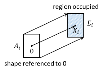
(a) Model for object $i$.

(b) Model for environment.

Figure 1: Model for environment based on randomly located and shaped objects.

It is unavoidable that initially as automated driving technologies are introduced, only a fraction of vehicles will be equipped with sensors and/or participate in collaborative sensing. Thus only the subset equipped with sensors can participate in collaborative sensing – we shall refer to such objects as sensors. Each object has an independent probability $p_{s}$ of being a sensor. Thus the locations of sensors, $\Phi^{s}$, correspond to an independent thinning [22] of $\Phi$, and so $\Phi^{s}\sim$HPPP$(\lambda^{s})$ where $\lambda_{s}=p_{s}\lambda$. For such objects we assume for simplicity that each has one sensor, and denote by $Y_{i}\in\operatorname*{\mathbb{R}}^{2}$ the relative placement of the sensor on object $i$ referenced to $X_{i}$, so the location of sensor $i$ is given by $X_{i}+Y_{i}\in E_{i}$. Each sensor $i$ is assumed to have a radial sensing support $S_{i}^{0}\subset\operatorname*{\mathbb{R}}^{2}$ referenced to the location of the sensor which is defined as follows.

Definition 1.

(Radial sensing support) The radial sensing support of a sensor $i$ referenced to the origin, $S_{i}^{0}$, is the set of locations that can be viewed if the sensor is located at $0$ and the LOS to the location is not obstructed. The set $S_{i}^{0}$ can be represented in polar coordinates as follows,

$$S_{i}^{0}=\big{\{}(r,\theta)\big{|}r\in[0,r_{\max}^{i}(\theta)],\theta\in[0,2\pi]\big{\}},$$ (1)

where $r_{\max}^{i}(\theta)$ is the maximum sensing range in direction $\theta$.

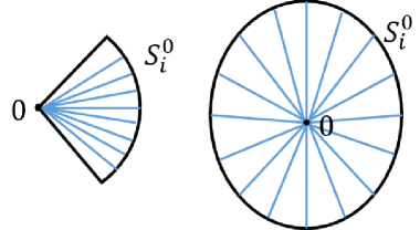
(a) Radial sensing support $S_{i}^{0}$

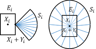
(b) Sensing support $S_{i}$

Figure 2: LABEL:sub@subfig:model:environment:object Radial support referenced to the origin $0$ and LABEL:sub@subfig:model:radial_support the sensing support of sensor $i$.

Fig. 2 illustrates examples of sector and omni-directional radial sensing supports. We denote by $S_{i}=\{X_{i}+Y_{i}\}\oplus S_{i}^{0}$ the sensing support of sensor $i.$ For an object, say $j$, which is not a sensor, we let $Y_{j}=0$ and $S_{j}^{0}=\emptyset$. The environment and the sensing field are thus modeled by an Independently Marked PPP (IMPPP), $\tilde{\Phi}$, which associates independent marks $M_{i}=(A_{i},Y_{i},S_{i}^{0})$ to each object $i$, i.e.,

$$\tilde{\Phi}=\big{\{}\big{(}X_{i},M_{i}\big{)},i\in{\operatorname*{\mathbb{N}}}^{+}\big{\}}.$$

Note that $(A_{i},Y_{i},S_{i}^{0})$ is independent of $X_{i}$, but $A_{i},Y_{i},S_{i}^{0}$ need not be mutually independent. Indeed if $i$ is a sensor, $Y_{i}\in A_{i}$ since the sensor should be mounted on the object. Also the distribution of the shape of objects with sensors, e.g., vehicles, can be different from that of other objects, e.g., pedestrians.

The aim of such general IMPPP model is to model all the objects in the environment, including vehicles, pedestrians, motorcycles, buildings, etc., thus we use a generalized HPPP model for the objects. Note that in practice vehicles follow the lanes on roads or parking lots, yet the analysis for such settings is similar to the simplified setting we consider. Furthermore comparisons via simulation of a detailed freeway model validate that the proposed HPPP model is a good approximation to study the performance of sensing in typical freeway and other scenarios. Our model may also apply to other (collaborative) sensing systems relying on wireless communication, but the model and analysis in this paper focuses on the unique characteristics of vehicular sensing, i.e., vehicles play the role of sensor, obstruction, and objects of interest at the same time.

II-B Model for Vehicle’s Region of Interest

We shall assume each sensing vehicle is interested in information within a certain range around it – usually measured in time, e.g., $t_{\operatorname*{interest}}$ sec. The actual spatial range depends on the vehicle’s speed $s$ and is given by $s\cdot t_{\operatorname*{interest}}$. We model a sensing vehicle’s region of interest as follows.

Definition 2.

(Region of interest) The region of interest for sensor vehicle $i$, $D_{i}$, is modeled for simplicity as a disc, $b(X_{i},r)$, centered at $X_{i}$ with radius $r=s\cdot t_{\operatorname*{interest}}$.

Note that for a vehicle located at the center of a multi-lane road, its region of interest can also be approximated by a rectangular set $[-s\cdot t_{\operatorname*{interest}},~{}~{}s\cdot t_{\operatorname*{interest}}]\times[-\frac{w_{\operatorname*{road}}}{2},\frac{w_{\operatorname*{road}}}{2}]$, where $w_{\operatorname*{road}}$ denotes the width of the road.

II-C Collaborative Sensing in an Obstructed Environment

Next we define a sensor’s coverage set given the environment and sensor model $\tilde{\Phi}$ as follows – see Fig. 3.

Definition 3.

(Sensor coverage set) For sensor $i$ with radial sensing support $S_{i}$ in the environment and sensor model $\tilde{\Phi}$, we let $E^{-i}=\underset{j:j\neq i}{\cup}E_{j}$ denote the environment excluding $E_{i}$. The coverage set of sensor $i$, $C_{i}(\tilde{\Phi})$, is then given by

$$C_{i}(\tilde{\Phi})=\big{\{}x\in S_{i}\big{|}x\in E_{i}\mbox{~{}or~{}}l_{X_{i}+Y_{i},x}\cap E^{-i}\subseteq\{x\}\big{\}},$$ (2)

where $l_{y,z}$ denotes the closed line segment between $y,z\in\operatorname*{\mathbb{R}^{2}}$. The coverage area of sensor $i$ is the area of its coverage set which we denote $|C_{i}(\tilde{\Phi})|$.

In the above definition, we assume that a sensor is aware of $E_{i}$, the space it occupies, i.e. no “self blocking”. Also $l_{X_{i}+Y_{i},x}\cap E^{-i}\subseteq\{x\}$ verifies that the LOS channel between the sensor at $X_{i}+Y_{i}$ and location $x$ is not blocked by other objects. A location $x\in C_{i}(\tilde{\Phi})$ may be in the void space or on the surface of an object. The coverage set of sensor $i$ represents the surrounding environment that it is able to view (on its own) under environmental obstructions.

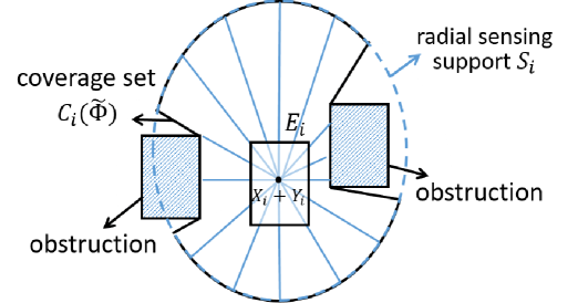
Figure 3: Coverage set of sensor $i$ in $\tilde{\Phi}$.

The expected coverage area of a typical sensor is given in the following theorem, where $C^{0}$ denotes the coverage set of a typical sensor shifted to the origin and $A^{0}$, $Y^{0}$ and $S^{0}$ are the associated shape, location of sensor, and radial support set, referred to the origin. The set $\{Y^{0}\}\oplus S^{0}\cap A^{0}$ denotes the region, if any, in the sensing support overlapping with the object, while $(\{Y^{0}\}\oplus S^{0})\backslash A^{0}=\{x|x\in\{Y^{0}\}\oplus S^{0},x\notin A^{0}\}$ is the region in the sensing support excluding the sensing object. Finally $A$ denotes a random set with the same distribution as the shape of objects and is independent of $A^{0}$. Their distributions may be different, since the latter is conditioned on an environmental object being a sensor, i.e., being a sensing vehicle.

Theorem 1.

Under our environment and sensor model $\tilde{\Phi}$ the expected coverage area of a typical sensor is given by

$${\operatorname*{\mathrm{E}}}\big{[}|C^{0}|\big{]}=\operatorname*{\mathrm{E}}[|(\{Y^{0}\}\oplus S^{0})\cap A^{0}|]\\ +{\operatorname*{\mathrm{E}}}\bigg{[}\int_{(\{Y^{0}\}\oplus S^{0})\backslash A^{0}}e^{-\lambda\cdot{\operatorname*{\mathrm{E}}}[|l_{Y^{0},x}\oplus\check{A}|]}dx\bigg{]},$$ (3)

where $\check{A}=\{x|-x\in A\}$.

For example if objects are modeled as discs of radius $r$, i.e., $A=b(0,r)$, with probability $1$, and the sensor is mounted at the center, i.e., $Y^{0}=0$, we have that $|l_{0,x}\oplus\check{A}|=\pi r^{2}+2r\cdot|x|$ (see [22]), so $\operatorname*{\mathrm{E}}\big{[}|C^{0}|\big{]}$ is straightforward to compute. The theorem shows how the coverage area of a single sensor decreases in the object density $\lambda$ since the probability of sensing a given location (the term inside integral) decreases exponentially in $\lambda$. The proof of Theorem 1 leverages straightforward stochastic geometric results and is relegated to the appendix.

II-D Sensor Coverage Area: Numerical and Simulation Results

Below we verify the robustness of our idealized analytical model by comparing the analytical results to a simulation of vehicles on a freeway. For the analytical model, the shape of all objects (vehicles) is a disc of radius $1.67\operatorname*{m}$, roughly corresponding to the area of a vehicle, and each has an omni-directional sensing support with radius $100\operatorname*{m}$. For the typical vehicle we limit its sensing support and coverage set to a rectangular region of interest centered on the vehicle, say $i$, such that

$$D_{i}=b(X_{i},100\operatorname*{m})\cap([-\infty,\infty]\times[X_{i}-12\operatorname*{m},X_{i}+12\operatorname*{m}]).$$ (4)

This is geared at capturing the fact that vehicles are mainly interested in sensing nearby road and sidewalks and $12\operatorname*{m}$ is roughly the width of three lanes.

Our simulations are based on the freeway scenario specified in [12] with $3$ lanes in each direction and lane widths of $4$ m. Vehicles are placed on each lane according to a linear Matérn process [23], i.e., randomly located but ensuring a minimum gap of $10$m among the centers of vehicles on the same lane. Vehicles are modeled as $4.8$m $\times 1.8$m rectangles, and the distance from the center locations to the lane center are uniformly distributed $\operatorname*{unif}[-1,1]$m. The coverage area does not include the region off the road.

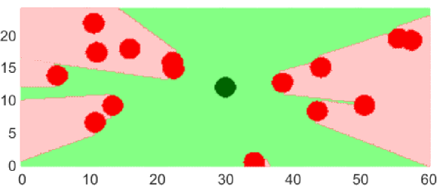
(a) Analytical model

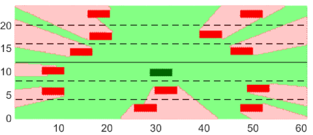
(b) Freeway simulation

Figure 4: Sensing of a typical vehicle in LABEL:sub@subfig:model:sensing:analysis analytical model and LABEL:sub@subfig:model:sensing:highway freeway simulation model. The green shapes are reference objects, the red shapes are obstructions, light green represents sensed region, light red indicates obstructed region.

Fig. 4 illustrates an example of sensing in our simplified analytical model and freeway simulation. The sensed and obstructed regions in the two models share similar characteristics.

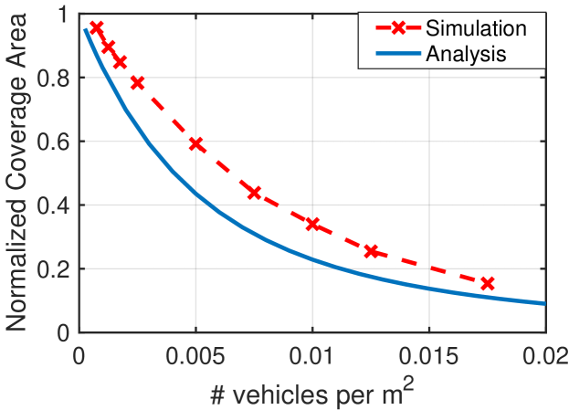
Figure 5: Coverage area of a typical vehicle normalized by the area of its sensing support.

Fig. 5 exhibits analytical and simulation results for the vehicle’s coverage area normalized by the area of sensing support scales versus vehicle density $\lambda$. Confidence intervals are not shown as they are negligible. As expected, with increased vehicle density, the sensor coverage area decreases due to increased obstructions. To reduce boundary effects, the simulation results correspond to the average sensor coverage area for vehicles in the two most central lanes. As can be seen the analytical and simulation results exhibit similar trends. At high vehicle densities, the coverage area of a single vehicle is heavily limited, i.e., covering less than $20\%$ of the sensing support. In an obstructed environment collaborative sensing will be critical to achieve better coverage over each vehicle’s region of interest. We consider this next.

III Benefits of Collaborative Sensing

The benefits of collaborative sensing are twofold: (1) it increases sensing redundancy/diversity leading to improved coverage, and (2) it improves coverage by effectively extending the sensing range. We consider two metrics for the performance of collaborative sensing: redundancy and coverage.

Sensing redundancy. We define sensing redundancy as the number of collaborative sensing vehicles that can view a location/object. The task of detecting/recognizing and tracking objects is facilitated if multiple sensors’ point of view are available, providing greater coverage and robustness to sensor/communication link failures.

Definition 4.

(Sensing redundancy for a location) Given an environment and sensing field, $\tilde{\Phi}$, and a subset of collaborating sensors $K\subseteq\Phi^{s}$, the sensing redundancy for a location $x$ is the number of sensors in $K$ that view $x$, denoted by

$$R(\tilde{\Phi},K,x)=\sum_{i:X_{i}\in K}\operatorname*{\mathbbm{1}}\big{(}x\in C_{i}(\tilde{\Phi})\big{)}.$$ (5)

In the most optimistic case $K=\Phi^{s}$, i.e., all sensors collaborate. The expected redundancy of a location in the void space is given by the results in the following theorem.

Theorem 2.

Given an environment and sensing field $\tilde{\Phi}$ and assuming all sensors collaborate, $K=\Phi^{s}$, the expected redundancy of a typical location $x$ in the void space is

$${\operatorname*{\mathrm{E}}}[R(\tilde{\Phi},\Phi^{s},x)|x\notin E]=\frac{p_{s}\cdot\lambda\cdot{\operatorname*{\mathrm{E}}}[|C^{0}\backslash A^{0}|]}{e^{-\lambda\cdot\operatorname*{\mathrm{E}}[|A|]}},$$ (6)

where ${\operatorname*{\mathrm{E}}}[|C^{0}\backslash A^{0}|]$ is given in the second term in Eq. 3.

The proof of this theorem included in the appendix follows from the definition of redundancy and a sensor’s coverage set.

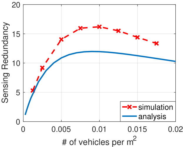
Figure 6: The expected sensing redundancy of a random void location versus object density. All vehicles participate in collaborating, i.e., $K=\Phi^{s}=\Phi$.

Fig. 6 exhibits the expected sensing redundancy of a typical location in the void space. As can be gleaned from our analytical results, sensing redundancy for a location is proportional to $p_{s}$ so we only exhibit results for $p_{s}=1$. At small densities sensors are not likely to be blocked thus redundancy first increases in the density of objects $\lambda$. However, at higher densities, the objects obstruct each other reducing the coverage area of each sensor and the resulting sensing redundancy. The simulation results show the expected redundancy of a random location in the central two lanes (see Section II-D), and exhibit similar trends as the analysis. Overall one can conclude that collaborative sensing will provide highest redundancy at moderate densities, i.e., this is where in principle collaborative sensing is most reliable and robust to sensor/communication failures.

Collaborative sensing coverage. A location in a vehicle’s region of interest is covered by collaborative sensing if the location can be reliably sensed, i.e., sensed by a sufficient number of collaborating sensors. We define the collaborative sensing coverage for a vehicle as follows.

Definition 5.

(Collaborative sensing coverage) Given an environment and sensing field $\tilde{\Phi}$, a minimum redundancy requirement $\gamma\in\operatorname*{\mathbb{N}}^{+}$ for reliable sensing of a location, a subset of collaborating sensors, $K\subseteq\Phi^{s}$, and sensor $i$’s region of interest $D_{i}$, the $\gamma$-coverage set of sensor $i$ is the region within $D_{i}$, which is covered by at least $\gamma$ sensors in $K$, denoted by

$$C_{c}(\tilde{\Phi},K,D_{i},\gamma)\mathrel{\ensurestackMath{\stackon[1pt]{=}{\scriptstyle\Delta}}}\big{\{}x\big{|}x\in D_{i},R(\tilde{\Phi},K,x)\geq\gamma\big{\}}.$$ (7)

The $\gamma$-coverage of sensor $i$ is the area of the $\gamma$-coverage set, $|C_{c}(\tilde{\Phi},K,D_{i},\gamma)|$. The normalized $\gamma$-coverage is the $\gamma$-coverage normalized by the area of the region of interest, $|C_{c}(\tilde{\Phi},K,D_{i},\gamma)|/|D_{i}|$.

The normalized $\gamma$-coverage can be interpreted as the fraction of $i$’s region of interest that can be reliably sensed. Denote by $D^{0}$ the possibly random region of interest associated with a typical sensing vehicle, and $A^{s}\subset\operatorname*{\mathbb{R}^{2}}$ a random set having the same distribution of the shape within a the region occupied by the sensor and is covered in the sensor’s support, i.e., $\{Y^{0}\}\oplus S^{0}\cap A^{0}$.

Approximation of the normalized $\gamma$-coverage. Denote by $\mkern 1.5mu\overline{\mkern-1.5muQ\mkern-1.5mu}\mkern 1.5mu(k,m)=\operatorname*{P}(N(m)\geq k)$, where $N(m)$ is a Poisson random variable with mean $m$. Denote by $\mkern 1.5mu\overline{\mkern-1.5muR\mkern-1.5mu}\mkern 1.5mu_{\operatorname*{void}}=\operatorname*{\mathrm{E}}[R(\tilde{\Phi},\Phi^{s},x)|x\notin E]$ the expected redundancy of a location in the void space as given in Eq. 6. The average $\gamma$-coverage can be approximated by

$$\operatorname*{\mathrm{E}}\big{[}|C_{c}(\tilde{\Phi},\Phi^{s},D^{0},\gamma)|\big{]}\approx$$

$$\operatorname*{\mathrm{E}}[|D^{0}\cap C^{0}\cap A^{0}|]\cdot\mkern 1.5mu\overline{\mkern-1.5muQ\mkern-1.5mu}\mkern 1.5mu(\gamma-1,\lambda^{s}\cdot\operatorname*{\mathrm{E}}[|A^{s}|])$$

$$+\operatorname*{\mathrm{E}}[|D^{0}\cap C^{0}\backslash A^{0}|]\cdot\mkern 1.5mu\overline{\mkern-1.5muQ\mkern-1.5mu}\mkern 1.5mu(\gamma-1,\mkern 1.5mu\overline{\mkern-1.5muR\mkern-1.5mu}\mkern 1.5mu_{\operatorname*{void}})$$

$$+\operatorname*{\mathrm{E}}[|D^{0}\backslash A^{0}|]\cdot\mkern 1.5mu\overline{\mkern-1.5muQ\mkern-1.5mu}\mkern 1.5mu(\gamma,\lambda^{s}\cdot\operatorname*{\mathrm{E}}[|A^{s}|])$$

$$+(\operatorname*{\mathrm{E}}[|D^{0}\backslash A^{0}|]\cdot e^{-\lambda\cdot\operatorname*{\mathrm{E}}[|A|]}-\operatorname*{\mathrm{E}}[|D^{0}\cap C^{0}\backslash A^{0}|])\cdot\mkern 1.5mu\overline{\mkern-1.5muQ\mkern-1.5mu}\mkern 1.5mu(\gamma,\mkern 1.5mu\overline{\mkern-1.5muR\mkern-1.5mu}\mkern 1.5mu_{\operatorname*{void}}).$$ (8)

This approximation is based on decomposing $D^{0}$ into various sets, see Fig. 7.

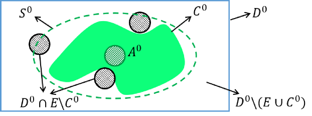
Figure 7: Decomposition of $D^{0}$ for collaborative sensing coverage approximation.

In particular, $D^{0}\cap C^{0}\cap A^{0}$ is the set occupied and sensed by the object, $D^{0}\cap C^{0}\backslash A^{0}$ is the set outside the object but sensed by the object, $D^{0}\cap E\backslash C^{0}$ is the set occupied by objects but not in $C^{0}$, and $D^{0}\backslash(E\cup C^{0})$ is the void space excluding $C^{0}$.

By Slivynak-Mecke theorem [22], the other objects as seen by the reference sensor follow an IMPPP with the same distribution as $\tilde{\Phi}$, so the locations of the other sensors follow HPPP$(\lambda^{s})$. The region covered by objects and sensors will each form a Boolean process [22]. For a random location $x$, the number of sensors occupying and sensing $x$ has a Poisson distribution with mean $\lambda^{s}\cdot\operatorname*{\mathrm{E}}[|A^{s}|]$, the number of objects occupying $x$ has a Poisson distribution with mean $\lambda\cdot\operatorname*{\mathrm{E}}[|A|]$. For a location in the void spacer, we will approximate the distribution of the redundancy by a Poisson distribution with mean $\mkern 1.5mu\overline{\mkern-1.5muR\mkern-1.5mu}\mkern 1.5mu_{\operatorname*{void}}$. $\mkern 1.5mu\overline{\mkern-1.5muR\mkern-1.5mu}\mkern 1.5mu_{\operatorname*{void}}$ is not conditioned on there being at typical sensor, thus $\mkern 1.5mu\overline{\mkern-1.5muR\mkern-1.5mu}\mkern 1.5mu_{\operatorname*{void}}$ can be different from the expected redundancy at a location $x\in D^{0}\backslash E$. In $C^{0}$ the reference object provides $1$ redundancy and other sensors should provide $(\gamma-1)$ redundancy, while in $D^{0}\backslash C^{0}$ the other sensors must provide $\gamma$ redundancy.

Based on the above approximation, the components of Eq. 8 are interpreted as follows:

• $\operatorname*{\mathrm{E}}[|D^{0}\cap C^{0}\cap A^{0}|]\cdot\mkern 1.5mu\overline{\mkern-1.5muQ\mkern-1.5mu}\mkern 1.5mu(\gamma-1,\lambda^{s}\cdot\operatorname*{\mathrm{E}}[|A^{s}|])$ is the area in $A^{0}$ that is occupied (and sensed) by $\gamma-1$ other sensors.

• $\operatorname*{\mathrm{E}}[|D^{0}\cap C^{0}\backslash A^{0}|]\cdot\mkern 1.5mu\overline{\mkern-1.5muQ\mkern-1.5mu}\mkern 1.5mu(\gamma-1,\mkern 1.5mu\overline{\mkern-1.5muR\mkern-1.5mu}\mkern 1.5mu_{\operatorname*{void}})$ is the area void space space in $C^{0}$ that is covered by $\gamma-1$ other sensors.

• $\operatorname*{\mathrm{E}}[|D^{0}\backslash A^{0}|]\cdot\mkern 1.5mu\overline{\mkern-1.5muQ\mkern-1.5mu}\mkern 1.5mu(\gamma,\lambda^{s}\cdot\operatorname*{\mathrm{E}}[|A^{s}|])$ is the area in $D^{0}\backslash A^{0}$ that is occupied (and sensed) by $\gamma$ sensors.

• $\operatorname*{\mathrm{E}}[|D^{0}\backslash A^{0}|]\cdot e^{-\lambda\cdot\operatorname*{\mathrm{E}}[|A|]}-\operatorname*{\mathrm{E}}[|D^{0}\cap C^{0}\backslash A^{0}|]$ is the area of void space in $D^{0}\backslash A^{0}$ excluding $C^{0}$, and $\mkern 1.5mu\overline{\mkern-1.5muQ\mkern-1.5mu}\mkern 1.5mu(\gamma,\mkern 1.5mu\overline{\mkern-1.5muR\mkern-1.5mu}\mkern 1.5mu_{\operatorname*{void}})$ is the probability that a location is covered by $\gamma$ other sensors.

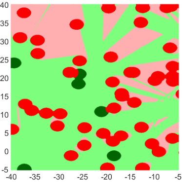
(a) Sensing in analytical model

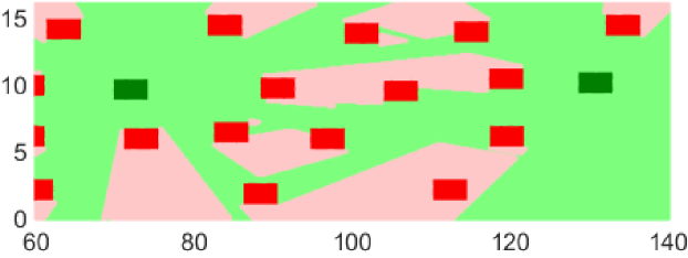
(b) Sensing in freeway scenario

Figure 8: Collaborative sensing in LABEL:sub@subfig:collaborative:scenario:analysis analytical model, and LABEL:sub@subfig:collaborative:scenario:highway freeway simulation. Dark green shapes represent sensors, red shapes are non-sensing objects. Light green region can be sensed via collaborative sensing, while light red region are obstructed and not sensed.

Fig. 8 illustrates collaborative sensing for our analytical model and the freeway simulation. In the analytical model, objects are modeled as randomly distributed discs and may overlap. The objects are randomly placed thus the region covered by collaborative sensing will also be the realization of a random shape. In the freeway simulation, vehicles are randomly distributed along lanes, such that there is no overlap. The environment is more ‘structured’, and thus so is the collaborative sensing coverage set, e.g., the space between lanes is less likely to be obstructed.

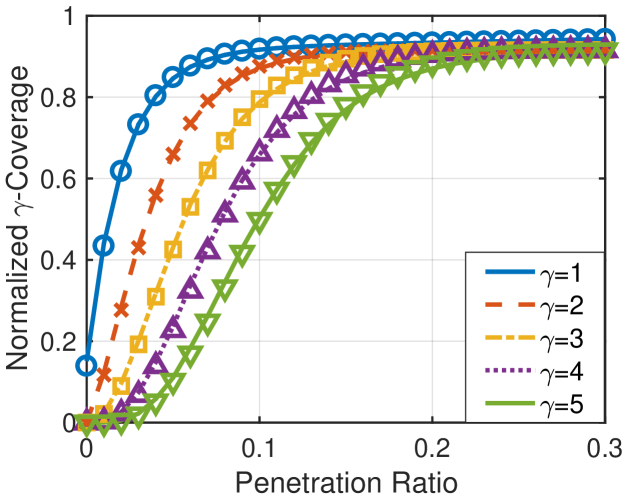
(a) Approximation validation

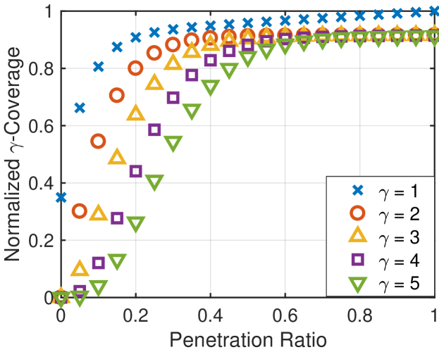
(b) Freeway simulation model

Figure 9: Normalized $\gamma$-coverage for different redundancy requirements $\gamma$. In LABEL:sub@subfig:collaborative:reliability:validation curves represent results from our approximation in Eq. 8 , markers are simulation of the analytical model. LABEL:sub@subfig:collaborative:reliability:simulation_gamma are freeway simulation results.

We validate the accuracy of our approximation in Fig. 9a, in which we consider a 2D infinite plane with $\lambda=0.01/{\operatorname*{m}}^{2}$. As can be seen the approximation in Eq. 8 is a good match for the analytical model. Fig. 9b exhibits the freeway simulation results, which show the same qualitative trend as the analytical results. As expected the minimum penetration to achieve a certain level of $\gamma$-coverage increases in the required diversity $\gamma$.

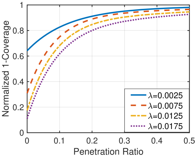
(a) Analytical Approximation

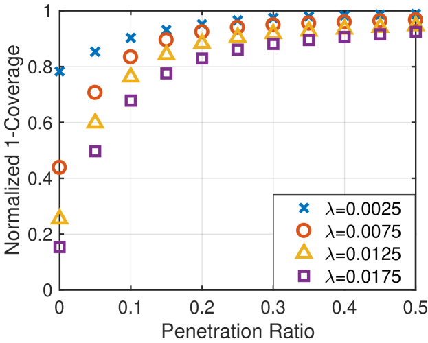
(b) Freeway simulation model

Figure 10: Normalized $1$-coverage: LABEL:sub@subfig:collaborative:reliability:analysis based on analytical approximation in Eq. 8, and LABEL:sub@subfig:collaborative:reliability:simulation obtained by simulation of freeway scenario.

Fig. 10 exhibits the expected normalized $1$-coverage for varying penetrations $p_{s}$ and vehicle densities $\lambda$. The freeway simulation results show the same trend as analytical results. Note that Eq. 8 is an approximation of the analytical model, which is different from our simulation of the freeway scenario. As expected, coverage increases monotonically in $p_{s}$. More importantly, collaborative sensing can greatly improve coverage even with a small penetration of collaborating vehicles, e.g., over $0.8$ coverage when $20\%$ of vehicles collaborate as compared to $0.2$ coverage without collaboration at a vehicle density $\lambda=0.0175/{\operatorname*{m}}^{2}$. Such results indicate that it would be beneficial to share sensor data even with only a subset of neighboring vehicles.

Despite the performance gains associated with vehicular collaborative sensing, achieving a high $\gamma$-coverage at low penetrations is difficult, especially for $\gamma>1$. Joint collaborative sensing with Road Side Units (RSUs) having sensing capabilities can help improve coverage, e.g., and RSU infrastructure could provide $100\%$ $1$-coverage if located above a freeway (no obstruction) if their sensing support covers the freeway. If $\gamma_{\operatorname*{rsu}}$ denotes the redundancy provided by RSU infrastructure, the gain in $\gamma$-coverage associated with joint vehicle/RSU collaboration is given by

$$\operatorname*{\mathrm{E}}\big{[}|C_{c}(\tilde{\Phi},\Phi^{s},D^{0},\gamma-\gamma_{\operatorname*{rsu}})|\big{]}-\operatorname*{\mathrm{E}}\big{[}|C_{c}(\tilde{\Phi},\Phi^{s},D^{0},\gamma)|\big{]}.$$ (9)

In Fig. 9b, for $\gamma_{\operatorname*{rsu}}=1$ and $p_{s}=0.1$, collaboration with RSUs improves $2$-coverage by over $0.25$. In summary the possibility of combining vehicular collaborative sensing with infrastructure (RSU) based sensing provides a natural avenue to improve coverage, especially at low penetrations, but possibly also at higher penetrations if $\gamma=2$ or higher diversity is desired.

Another setting our analytical framework can shed light on is how the collaborative sensing coverage scales in the obstruction density when the sensor density is fixed. One example of such a setting might be some freeway on ramps where vehicles entering the freeway are primarily non-sensing capable. Fig. 11 exhibits how the $1$-coverage scales in the obstruction density based on the approximation in Eq. 8. As can be seen the $1$-coverage decreases approximately linearly in the obstruction density. Collaborative sensing with RSUs may be required to ensure coverage in such scenarios.

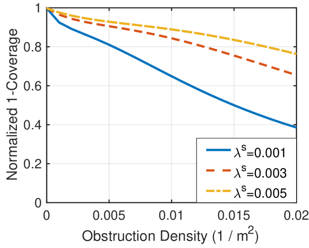
Figure 11: Normalized $1$-coverage for different obstruction densities, $\lambda-\lambda^{s}$. Sensor density $\lambda^{s}$ is fixed.

IV Network Capacity Scaling for Collaborative Sensing Applications

In this section we study the network capacity requirements for collaborative sensing. We envisage both V2V and V2I connectivity might be used to enable collaborative sensing in automotive settings. This might be critical to meet reliability and coverage requirements as we transition from legacy systems. In particular when the penetration of collaborative sensing vehicles is limited, the V2V links/paths required to share collaborative sensing data may be blocked / unavailable, particularly when line of sight based links are used such as mmWave or optical based links. When this is the case, V2I connectivity, e.g., LTE based links, could serve as the fallback to share critical sensing/manouvering information. Below we study the V2I fallback capacity scaling for collaborative sensing settings.

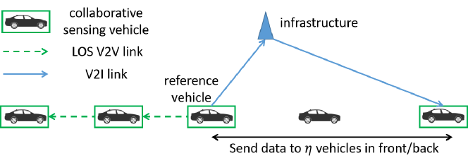
Figure 12: Collaborative sensing of vehicles in a single lane with V2V + V2I network. Vehicle uses V2I to relay data when LOS V2V links are blocked.

We consider vehicles on a single lane assisted by infrastructure deployed along the road. Vehicles move at a constant velocity $s$. Each sensing vehicle has a region of interest, $t_{\operatorname*{interest}}$ sec, in both forward and backward directions. We shall consider the worst case scenario, i.e., the density of vehicles is high and the gap between (the centers of) vehicles in the same lane is the minimum gap for safe driving, $t_{\operatorname*{gap}}$ sec and the inter-vehicle gap is $s\cdot t_{\operatorname*{gap}}\operatorname*{m}$. The density of vehicle is thus given by $\lambda_{\operatorname*{v}}=\frac{1}{s\cdot t_{\operatorname*{gap}}}$. We assume vehicles need to receive data from all vehicles in their range of interest, and by symmetry vehicle also need to send data to all vehicles in their range of interest. A sensing vehicle thus needs to send data to $\eta=\lfloor\frac{t_{\operatorname*{interest}}}{t_{\operatorname*{gap}}}\rfloor$ other vehicles in front and behind it, see Fig. 12.

A vehicle has LOS V2V communication channels to the neighboring vehicles in front and back. A non collaborating vehicle thus blocks the V2V relay path along the chain of vehicles. If a LOS V2V relay path is not available, we assume the reference vehicle relays data through the infrastructure and the receiving vehicle can then further relay data to other vehicles via available V2V links (V2I + V2V relay). We assume the message a vehicle sends to other vehicles is the same, thus a vehicle only needs to upload its data to the infrastructure at most once. The infrastructure can then relay the message to other vehicles requiring the message via either unicast or broadcast. If using unicast, infrastructure needs to send the message to every vehicle located in its service region, which requires the message and cannot get the message via V2V / V2I + V2V relay.

Let $N_{\operatorname*{UL}}$ and $N_{\operatorname*{DL}}^{\operatorname*{U}}$ be random variables denoting the number of uplink and unicast downlink V2I transmissions required to share data of a typical sensing vehicle. The expected required V2I uplink capacity $c_{\operatorname*{UL}}$ and V2I downlink capacity for broadcast, $c_{\operatorname*{DL}}^{\operatorname*{B}}$, and unicast, $c_{\operatorname*{DL}}^{\operatorname*{U}}$, are given in the following theorem.

Theorem 3.

Consider a single lane model, with a density of vehicles is $\lambda_{\operatorname*{v}}$, where each sensing vehicle share data with $\eta=\lfloor t_{\operatorname*{interest}}/t_{\operatorname*{gap}}\rfloor$ vehicles in front and back. The V2I capacity requirements on a infrastructure serving the linear road segment of length $d\operatorname*{m}$ are given by

$$c_{\operatorname*{UL}}=c_{\operatorname*{DL}}^{\operatorname*{B}} =p_{s}\cdot\lambda_{\operatorname*{v}}\cdot d\cdot\operatorname*{\mathrm{E}}[N_{\operatorname*{UL}}]\cdot\nu,$$ (10)

$$c_{\operatorname*{DL}}^{\operatorname*{U}} =p_{s}\cdot\lambda_{\operatorname*{v}}\cdot d\cdot\operatorname*{\mathrm{E}}[N_{\operatorname*{DL}}^{\operatorname*{U}}]\cdot\nu,$$ (11)

where

$$\operatorname*{\mathrm{E}}[N_{\operatorname*{UL}}]=1-\big{(}\sum_{k=0}^{\eta}p_{s}^{k}\cdot(1-p_{s})^{\eta-k}\big{)}^{2},$$ (12)

$$\operatorname*{\mathrm{E}}[N_{\operatorname*{DL}}^{\operatorname*{U}}]=\begin{cases}2(\eta-1)p_{s}(1-p_{s}),&\text{if }\eta\geq 2,\\ 0,&\text{otherwise}\end{cases}.$$ (13)

The development of this result can be found in the appendix. The above results convey the average capacity requirements on V2I infrastructure. Unfortunately in a single lane setting a single non-collaborating vehicle can block the V2V LOS links/paths amongst a large number of vehicles and result in a burst of V2I traffic especially at high penetrations, e.g., when vehicles in front and back of the non-collaborating vehicle are all collaborating. The required V2I capacity to handle such bursts can thus be much higher.

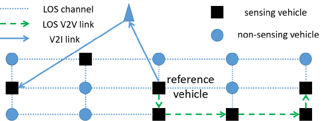
Figure 13: Collaborative sensing of vehicles in a single lane using V2V + V2I, with V2V relay assistance from vehicles in the two neighboring lanes.

The single lane relaying scenario studied above is a worst case, i.e., data can only be relayed by vehicles on the same lane. One can also consider scenarios where in addition collaborative vehicles on either of two neighboring lanes participate in V2V relaying. LOS links among vehicles on neighboring lanes are less likely to be blocked, but LOS links to distant vehicles in neighboring lanes will see larger path loss and may experience more interference, e.g., from transmissions of vehicles in the same lane. Thus for simplicity suppose vehicles only communicate with the closest vehicle in a neighboring lane and consider the simple grid connectivity model shown in Fig. 13. Each node on the grid corresponds to a vehicle, and each row represents a lane. Vehicles have LOS channels to neighboring vehicles on the grid. For comparison purposes we suppose, as before, that a reference vehicle needs to send data to $\eta$ vehicles in front and back in the same lane. Vehicles can receive data via V2V links if there is an LOS V2V relay path on the grid. To limit the number of hops and associated delays we assume that a relay path can not include links in both forward and backward directions.

Based on this model, whether vehicles in the $(k+1)^{th}$ column from the reference vehicle can receive data via V2V links depends on whether the vehicles in the $(k+1)^{th}$ column are collaborating and can get data from vehicles in the $k^{th}$ column. In this setting one can again compute the expected V2I capacity requirements to deliver data to vehicles in each column and thus the total capacity requirements as a function of $\eta$ and $p_{s}$ – a detailed analysis is included in the appendix.

IV-A Numerical Results

Fig. 14 exhibits how the V2I capacity, $c_{\operatorname*{UL}}$, $c_{\operatorname*{DL}}^{\operatorname*{B}}$ and $c_{\operatorname*{DL}}^{\operatorname*{U}}$, normalized by $\lambda_{\operatorname*{v}}\cdot d\cdot\nu$ and the average V2V throughput per sensing vehicle normalized by V2V throughput at $p_{s}=1$, vary with $p_{s}$ in single lane setting and in the single lane assisted by vehicles in neighboring lanes setting. The results correspond to the case where $\eta=5$. An increase in $p_{s}$ causes an increase in the number of vehicles participating in collaborative sensing but also results in improved V2V connectivity. When $p_{s}$ is small, both the number of collaborative sensing vehicles and the capacity per sensing vehicle increase, thus V2I traffic increases. However at higher penetrations, V2V connectivity improves and the V2I capacity requirements of a sensing vehicle decreases, resulting in lower and eventually negligible V2I traffic. Comparing the results with and without assistance from vehicles in neighboring lanes, we observe, as expected, that V2I traffic is smaller when vehicles in neighboring lanes can help relay data. The V2V throughput per sensing vehicle increases with $p_{s}$. However if vehicles in neighboring lanes assist with V2V relaying, the V2V throughput is higher than that in the single lane scenario, and the $c_{\operatorname*{V2V}}$ can be higher than the V2V throughput at full penetration.

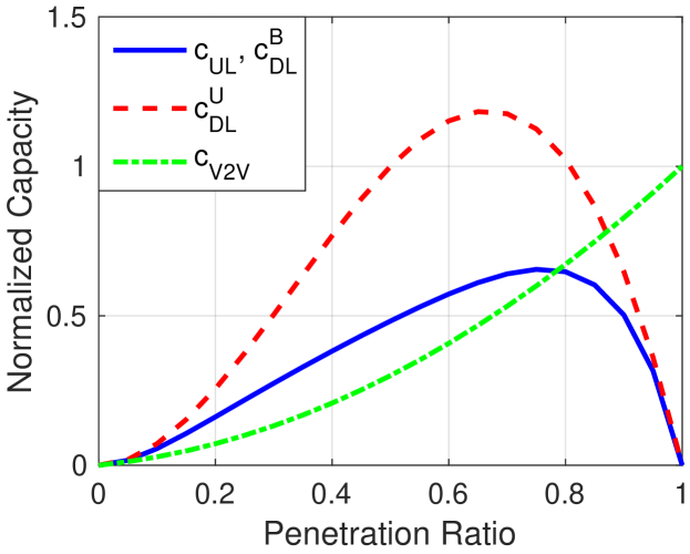
(a) Single lane

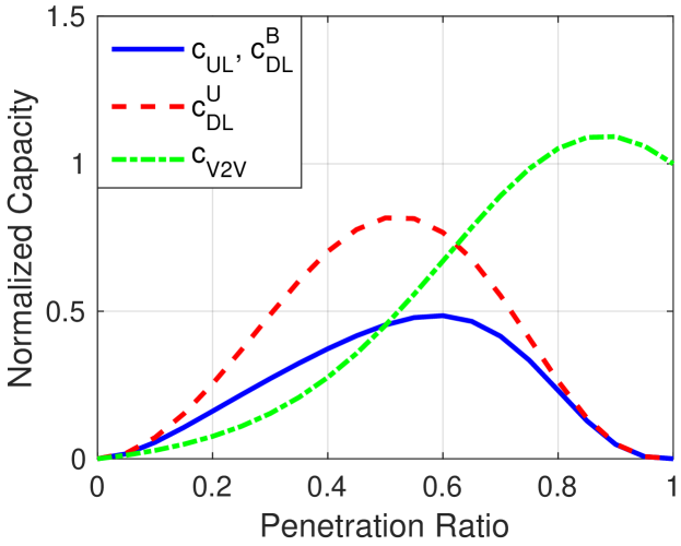
(b) Single lane assisted by vehicles in neighboring lanes

Figure 14: How V2I capacity requirements, normalized by $\lambda_{\operatorname*{v}}\cdot d\cdot\nu$, scale with $p_{s}$ in LABEL:sub@subfig:scalability:v2i:1d:capacity single lane and LABEL:sub@subfig:scalability:v2i:2d:capacity single lane assisted by vehicles in neighbor lanes. $c_{\operatorname*{UL}}$ is uplink capacity, $c_{\operatorname*{DL}}^{\operatorname*{B}}$ and $c_{\operatorname*{DL}}^{\operatorname*{U}}$ are downlink capacity using broadcast and unicast. $c_{\operatorname*{V2V}}$ is V2V throughput per sensing vehicle normalized by the V2V throughput at full penetration, $p_{s}=1$.

In summary the V2I traffic resulting from collaborative sensing data would be highest at intermediate penetrations, e.g., ranging from $0.5$ to $0.7$, but eventually would decline once most vehicles participate in both collaborative sensing and V2V networking. This suggests an evolution path where V2I resources are initially critical to safety-related services like collaborative sensing, but eventually at high penetrations of sensing vehicles, traffic can be effectively offloaded to the V2V network, e.g., in the single lane assisted by neighboring lanes, $c_{\operatorname*{UL}},c_{\operatorname*{DL}}^{\operatorname*{B}}$ per vehicle is less than $0.25\nu$ if $p_{s}>0.8$, and the infrastructure may transition to supporting non-safety-related services, e.g., mobile high data rate entertainment and dynamic digital map updates. These results are likely robust to improved models, yet more detailed analysis based on more accurate V2V mmWave channel and networking models would be required to provide more accurate quantitative assessment.

V Impact of Dynamics on Collaborative Sensing

In the previous sections we studied how collaborative sensing improves coverage for a snapshot of the environment by providing spatial diversity in sensing, i.e., sensor data for locations and objects from different points of view. In addition, collaborative sensing can improve sensing performance by utilizing temporal diversity in sensing. Objects in the environment are moving thus the environment is dynamic, e.g., vehicles’ regions of interest, blockage fields, and the sensor coverage sets are varying with time. Sensor data measured at different time provides possibly different information regarding the environment, thus sensors can exploit temporal diversity for sensing and tracking of objects in the environment.

V-A Temporal Dynamic Environment and Sensing Model

We shall consider extending the environment and sensing model proposed in Section II to capture temporal dynamics. We let $X_{i}$ be the location of object $i$ at time $0$, and denote by

$$\Phi^{d}(t)=\{X_{i}^{d}(t),i\in{\operatorname*{\mathbb{N}}}^{+}\}$$

the locations of objects at time $t$, where $X_{i}^{d}(t)$ is the location of object $i$ at time $t$. Suppose the movements of objects are IID and independent of the locations of objects (during the time interval of interest). Since the objects’ locations follow $\Phi\sim\operatorname*{HPPP}(\mathrm{\lambda})$ it follows by the Displacement Theorem [22] that the locations of objects at any time $t$ will remain an HPPP process, i.e., for all $t>0$,

$$\Phi^{d}(t)\sim\operatorname*{HPPP}(\lambda).$$

For simplicity we suppose the shape, location of sensor on the object, and the radial sensing support of the sensor, $M_{i}=(A_{i},Y_{i},S_{i}^{0})$, do not change with time, e.g., objects do not rotate. Denote by

$$E_{i}^{d}(t)=X_{i}^{d}(t)\oplus A_{i}$$ (14)

the region occupied by object $i$ at time $t$, and

$$S_{i}^{d}(t)=X_{i}^{d}(t)\oplus S_{i}^{0}$$ (15)

the sensing support of sensor $i$ at $t$. The environment and sensing sensing field at $t$ is then given by

$$\tilde{\Phi}^{d}(t)=\big{\{}\big{(}X_{i}^{d}(t),(A_{i},Y_{i},S_{i}^{0})\big{)},i\in{\operatorname*{\mathbb{N}}}^{+}\big{\}},$$

and the model for the temporal dynamics of the environment and sensing capabilities is denoted by

$$\boldsymbol{\tilde{\Phi}^{d}}=\big{(}\tilde{\Phi}^{d}(t),t\in{\operatorname*{\mathbb{R}}}^{+}\big{)}.$$

We let $\Phi^{s}$ denote the locations of collaborating sensors at time $0$.

The coverage set of sensor $i$ at time $t$, denoted $C_{i}^{d}(\boldsymbol{\tilde{\Phi}^{d}},t)$, is given by

$$C_{i}^{d}(\boldsymbol{\tilde{\Phi}^{d}},t)=\\ \big{\{}x\in S_{i}^{d}(t)\big{|}x\in E_{i}^{d}(t)\mbox{~{}or~{}}l_{X_{i}^{d}(t)+Y_{i},x}\cap E^{-i,d}(t)\subseteq\{x\}\big{\}},$$ (16)

where $E^{-i,d}(t)={\cup}_{j\neq i}E_{j}^{d}(t)$ is the blockage set associated with objects other than $i$ at time $t$.

We let $D_{i}^{d}(t)\subseteq\operatorname*{\mathbb{R}^{2}}$ denote sensor $i$’s region of interest at time $t$. We shall define the objects that a sensor needs to sense at time $t$ as follows.

Definition 6.

(Objects of interest at time $t$) The objects of interest of sensor $i$ at time $t$ are the objects which overlap with sensor $i$’s region of interest at $t$, denoted by $O_{i}^{d}(t)$, and given by

$$O_{i}^{d}(t)=\big{\{}j\in{\operatorname*{\mathbb{N}}}^{+}\big{|}E_{j}^{d}(t)\cap D_{i}^{d}(t)\neq\emptyset\big{\}}.$$ (17)

V-B Sensing Redundancy and Coverage Resulting from Temporal Dynamics

We suppose an object $i$ is sensed by object $j$ at time $t$ if sensor $j$ senses any part of $i$, i.e.,

$$C_{j}^{d}(\boldsymbol{\tilde{\Phi}^{d}},t)\cap E_{i}^{d}(t)\neq\emptyset.$$

Sensors can track the states of objects in the environment, e.g., locations, velocity, acceleration, etc, and thus have a good estimate of the objects even when the objects are blocked for some time. For simplicity we assume an object is tracked by a sensor at $t$ if the object has been sensed in time interval $[t-\tau,t]$, where $\tau$ is the maximum time window for reliable tracking without new sensor data.

The spatio-temporal sensing redundancy of an object can then be defined as follows.

Definition 7.

(Spatio-temporal object sensing redundancy) Given an environment and sensing model $\boldsymbol{\tilde{\Phi}^{d}}$, a fixed subset of collaborating sensors, $K\subseteq\Phi^{s}$, and assuming an object can be sensed if it has been sensed within a time period $\tau$, the object sensing redundancy of sensor $i$ at time $t$ is given by

$$R^{\operatorname*{o},d}(\boldsymbol{\tilde{\Phi}^{d}},K,i,t,\tau)=\\ \sum_{j:X_{j}\in K}\operatorname*{\mathbbm{1}}\big{(}\exists z\in[t-\tau,t]\mbox{~{}s.t.~{}}E_{i}^{d}(z)\cap C_{j}^{d}(\boldsymbol{\tilde{\Phi}^{d}},z)\neq\emptyset\big{)}.$$ (18)

Given the above definition of spatio-temporal sensing redundancy we can define the $(\gamma,\tau)$-object coverage as follows.

Definition 8.

($(\gamma,\tau)$-object coverage) Given an environment and sensing field $\boldsymbol{\tilde{\Phi}^{d}}$, a minimum redundancy requirement $\gamma\in\operatorname*{\mathbb{N}}^{+}$ for reliable sensing of an object, a subset of collaborating sensors, $K\subseteq\Phi^{s}$, and sensor $i$’s objects interest $O_{i}^{d}$, the $\gamma$-coverage object set of sensor $i$ is the set of objects of interest at time $t$ which are covered by at least $\gamma$ sensors in $K$, denoted by

$$C_{c}^{d}(\tilde{\Phi}^{d},K,O_{i}^{d},\gamma,t,\tau)\mathrel{\ensurestackMath{\stackon[1pt]{=}{\scriptstyle\Delta}}}\big{\{}j\in O_{i}^{d}(t)\big{|}R^{d}(\tilde{\Phi}^{d},K,j,t,\tau)\geq\gamma\big{\}}.$$ (19)

The $(\gamma,\tau)$-object coverage is proportion of the objects of interest that are in the $\gamma$-coverage set, i.e.,

$$\frac{|C_{c}(\tilde{\Phi},K,O_{i}^{d},\gamma,t,\tau)|}{|O_{i}^{d}(t)|}.$$ (20)

V-C Performance of Collaborative Sensing Utilizing Spatio-temporal Diversity

The relative movement of neighboring vehicles driving in the same direction would typically be small, e.g., the relative locations of vehicles in a fleet may be stable most time. Such slow relative movement facilitates the communication amongst the vehicles, but limits the temporal diversity in the sensing of vehicles moving in the same direction. The sensing coverage of collaborative sensing for vehicles moving in the same direction may fail to change quickly with time and obstructed vehicles will remain unseen. By comparison RSUs and vehicles moving in the opposite direction will see fast relative movements to a given flow of vehicles and have improved sensing coverage with temporal diversity. We have shown in [24] that RSUs can have an almost unobstructed view of the road if located well above the vehicles. In practice, RSUs may be low, e.g., to save cost, and vehicles are of different dimension, thus the sensing of vehicles can be obstructed. However RSUs may benefit from temporal sensing diversity with respect to a flow of vehicles. The relative velocity of vehicles moving in the opposite direction is large, i.e., twice the typical speed of a vehicle, which increases temporal diversity. However such high relative speeds can make it difficult to establish reliable high rate links, e.g., in the mmWave band.

Let us evaluate the performance of collaborative sensing in the presence of such relative motions via simulation in a freeway scenario. We extend the simulation setting in Section II-D. Sensing and communication capable RSUs are located along one side of the road at an even spacing, denoted by $d_{\operatorname*{rsu}}$. The RSUs are at a distance $d_{\operatorname*{road}}$ from the edge of the road and the height of RSUs is $h_{\operatorname*{rsu}}$. Denote by $r_{\operatorname*{rsu}}$ the sensing range of RSUs, $r_{\operatorname*{v}}$ the sensing range of vehicles. Both RSUs and vehicles have the same communication range $r_{\operatorname*{comm}}$. Vehicles are moving at the same speed $s$. We shall refer to the direction of the lanes close to RSUs as the ‘nearby’ direction, and the other direction as the ‘opposite’ direction, see Fig. 15.

Figure 15: Freeway simulation scenario for RSU assisted collaborative sensing with temporal dynamics.

We consider different collaborative sensing schemes, i.e., 1) base case: collaborate with only vehicles moving in the same direction. The communication channel is stable, yet the set of collaborating sensors is limited. 2) RSU: in addition vehicles communicate with sensing capable RSUs. 3) opposite: vehicles communicate with vehicles moving in the same direction and in the opposite direction.

(a) Collaboration with RSUs and/or vehicles in the nearby direction

(b) Collaboration with RSRUs and/or vehicles in the opposite direction

Figure 16: The $(1,\tau)$-object coverage of collaborative sensing with vehicles driving in the same direction and RSUs for vehicles moving in LABEL:sub@subfig:temporal:rsu_coverage:original the original direction, and LABEL:sub@subfig:temporal:rsu_coverage:opposite the opposite direction.

Fig. 16 illustrates the $(1,\tau)$-object coverage of collaborative sensing under our three different collaboration schemes and different $\tau$. RSUs are uniformly deployed along the road, providing a $1$-coverage of the road, e.g., $r_{\operatorname*{rsu}}=200\operatorname*{m}$, $d_{\operatorname*{rsu}}=400\operatorname*{m}$. We assume $r_{\operatorname*{interest}}=200\operatorname*{m}$, $d_{\operatorname*{road}}=2\operatorname*{m}$, $r_{\operatorname*{v}}=200\operatorname*{m}$, $s=20\operatorname*{m}/s$. The communication range is $r_{\operatorname*{comm}}=500\operatorname*{m}$, which is enough for a vehicle to communicate with all sensors having relevant sensor data. We set $h_{\operatorname*{rsu}}=1\operatorname*{m}$, which is lower than the heights of vehicles, i.e., typically $1.5\operatorname*{m}$ for sedans or higher for other vehicles. Such assumption on $h_{\operatorname*{rsu}}$ is mainly used to make the sensors subject to obstructions to study the impact of temporal diversity. The base case is that vehicles collaborate with other vehicles moving in the same direction.

First let us consider collaborative sensing without temporal diversity, i.e., $\tau=0\sec$. From the simulation results in Fig. 16 we can see sensing coverage increases with spatial diversity, i.e., collaboration with RSUs and/or vehicles in the opposite direction improves the sensing coverage. If we compare the coverage when only RSUs or neighbor vehicles are used, we can see that collaborating with only RSUs provides larger gain at low penetrations while collaborating with neighbor vehicles direction works better at high penetrations. As expected, collaborating with both RSUs and vehicles in the opposite direction provides most temporal diversity and thus most gain.

When temporal diversity in sensing is utilized, i.e., RSUs and vehicles in the opposite direction track objects using previous measurements, coverage can be further improved. In fact the coverage increases with $\tau$. Note that collaborating with RSUs and utilizing temporal diversity alone can already provide a relative high coverage, e.g., over $95\%$. This indicates that RSUs can have a good coverage of the environment by tracking objects even when RSUs are not located higher than all objects and are subject to objects. A comparison of coverage for vehicles moving in different directions shows that RSUs provide better temporal diversity for sensing vehicles moving in the further away lanes. The reason is that the obstructions in the nearby lanes have larger relative movements, thus RSUs will see larger temporal diversity in the obstruction field.

VI Conclusion

Collaborative sensing can greatly improve a vehicle’s sensing coverage. V2V collaborative sensing could improve the sensing coverage from $20\%$ to $80\%$ at $20\%$ penetration and we can further improve the coverage using both V2V and V2I collaborative sensing. However, collaborative sensing suffers at low penetrations due to, both a lack of available collaborators, and communication blockages for (mmWave) V2V relaying paths. Access to V2I connectivity will thus be important to provide communication for collaborative sensing when V2V relaying paths are unavailable. At higher penetrations, the average V2I traffic is low, but the infrastructure should still have the ability to support traffic bursts when the V2V network of collaborating vehicles becomes disconnected.

To provide higher coverage one might consider supporting joint collaborative sensing amongst vehicles and RSUs with both sensing and communication capabilities. With sufficient RSU density and unobstructed placements, one can ensure $100\%$ $1$-coverage by collaborating only with RSUs. The associated capacity requirement can also be much smaller than collaboration with vehicles: vehicles receive data from one RSU instead of all neighboring vehicles. However sensing based only on RSUs deployed with $100\%$ $1$-coverage might not provide enough sensing redundancy and deploying even more RSUs to provide diversity would be costly. Furthermore, in order to navigate in a variety of environments, vehicles will need to have their own sensing capabilities which should clearly be leveraged. Thus we see the combination of vehicular/RSU collaborative sensing as the most cost effective way to achieve high coverage in vehicular automated driving applications – in particular say for high speed automated highways.

-A Proof of Theorem 1

The locations associated marks of the objects, $\tilde{\Phi}$, follow an IMPPP, thus the occupied space can be modeled by a Boolean Process [22]. One can also formally define the distribution as seen by a typical vehicle referred to the origin $0$. Let $Z^{0}=(0,M^{0})$, $M^{0}=(A^{0},Y^{0},S^{0})$, denote the typical vehicle. We let

$$f(x,z^{0},\tilde{\phi}\backslash\{z^{0}\})=\operatorname*{\mathbbm{1}}(x\in c^{0})$$ (21)

be the indicator function that location $x$ is in the coverage set of the typical sensor $z^{0}$, where $\tilde{\phi}\backslash\{z^{0}\}$ denotes the other objects in the environment excluding $z^{0}$. The expected area of coverage set of a typical vehicle is then given by,

$$\begin{split}\operatorname*{\mathrm{E}}[|C^{0}|]&={\operatorname*{\mathrm{E}}}\bigg{[}\int_{x\in\operatorname*{\mathbb{R}^{2}}}f(x,Z^{0},\tilde{\Phi}\backslash\{Z^{0}\})dx\bigg{]}\\ &=\int_{x\in\operatorname*{\mathbb{R}^{2}}}\int_{m\in\mathbb{M}}\int_{\tilde{\phi}}f(x,\tilde{\phi}\backslash\{z\},z)P_{z}^{!}(d\tilde{\phi})F_{M^{0}}(dm)dx,\end{split}$$ (22)

where $\mathbb{M}$ is the support of $M^{0}$, $P_{z}^{!}(\cdot)$ is the reduced Palm distribution of $\tilde{\Phi}$ given a typical object is $z=(0,m)$, i.e., the distribution of other objects in the environment as seen by a typical object[22]. For a Boolean Process, it follows by Slivnyak-Mecke theorem [22] that the reduced Palm distribution is the same as that of the original Boolean Process. Thus we have

$$\begin{split}&\int_{\tilde{\phi}}f(x,z,\tilde{\phi}\backslash\{z\})P_{z}^{!}(d\tilde{\phi})=\int_{\tilde{\phi}}f(x,z,\tilde{\phi})P_{\tilde{\Phi}}(d\tilde{\phi})\\ \stackrel{{\scriptstyle(1)}}{{=}}&\operatorname*{\mathbbm{1}}(x\in(\{y\}\oplus s)\cap a)+\operatorname*{\mathbbm{1}}(x\in(\{y\}\oplus s)\backslash a)e^{-\lambda{\operatorname*{\mathrm{E}}}_{A}[|l_{y,x}\oplus\check{A}|]},\end{split}$$ (23)

where $(\{y\}\oplus s)\backslash a$ is the sensing support of the typical sensor excluding the region $a$ covered by the sensor itself. In equality $(1)$ we have used the fact that for a Boolean Process, the number of objects intersecting a compact convex shape, e.g., $l_{y,x}$, has a Poisson distribution with mean $\lambda\cdot\operatorname*{\mathrm{E}}_{A}[|l_{y,x}\oplus\check{A}|]$, $\check{A}=\{x|-x\in A\}$ [22]. Thus substituting the result in Eq. 23 into Eq. 22 we get Eq. 3.

-B Proof of Theorem 2

The locations of the objects follow an HPPP and the environment can be modeled as an IMPPP thus the environment is homogeneous in space. Without loss of generality we consider the redundancy of location $0$. By definition, we have

$$\operatorname*{\mathrm{E}}[R(\tilde{\Phi},\Phi^{s},0)|0\notin E]=\frac{\operatorname*{\mathrm{E}}[R(\tilde{\Phi},\Phi^{s},0)\cdot\operatorname*{\mathbbm{1}}(x\notin E)]}{\operatorname*{P}(0\notin E)}$$ (24)

Since the region occupied by objects follows the Boolean Process thus the probability that $0$ is not occupied by objects is given by, see [22],

$$\operatorname*{P}(0\notin E)=e^{-\lambda\cdot\operatorname*{\mathrm{E}}[|A|]}.$$ (25)

We let $h(x_{0},x,m,\tilde{\phi}\backslash\{(x,m)\})$ be the indicator function that location $x_{0}$ is in the void space and sensed by object $(x,m)$, for the given environment excluding the reference object, i.e., $\tilde{\phi}\backslash\{(x,m)\}$. $\operatorname*{\mathrm{E}}[R(\tilde{\Phi},\Phi^{s},0)\cdot\operatorname*{\mathbbm{1}}(0\notin E)]$ is then given by,

$$\operatorname*{\mathrm{E}}[R(\tilde{\Phi},\Phi^{s},0)\cdot\operatorname*{\mathbbm{1}}(0\notin E)]$$

$$= \operatorname*{\mathrm{E}}\bigg{[}\sum_{(X_{i},M_{i})\in\tilde{\Phi},X_{i}\in\Phi^{s}}h\big{(}0,X_{i},M_{i},\tilde{\Phi}\backslash\{(X_{i},M_{i})\}\big{)}\bigg{]}$$

$$= p_{s}\lambda\int_{x\in\operatorname*{\mathbb{R}^{2}}}\int_{m\in\mathbb{M}}\int_{\tilde{\phi}}h(0,x,m,\tilde{\phi})P_{(x,m)}^{!}(d\tilde{\phi})F_{M}(dm)dx$$

$$\stackrel{{\scriptstyle(1)}}{{=}} p_{s}\lambda\int_{x\in\operatorname*{\mathbb{R}^{2}}}{\operatorname*{\mathrm{E}}}_{M,\tilde{\Phi}}\big{[}h(0,x,M,\tilde{\Phi})\big{]}dx$$

$$\stackrel{{\scriptstyle(2)}}{{=}} p_{s}\lambda\int_{x\in\operatorname*{\mathbb{R}^{2}}}{\operatorname*{\mathrm{E}}}_{M,\tilde{\Phi}}\big{[}h(-x,0,M,\tilde{\Phi})\big{]}dx$$

$$\stackrel{{\scriptstyle(3)}}{{=}} p_{s}\lambda\cdot\operatorname*{\mathrm{E}}[|C^{0}\backslash A^{0}|].$$ (26)

The equality $(1)$ follows for Slivnyak-Mecke theorem [22]. Equality $(2)$ follows from the spatial homogeneity of the environmental model thus we have that

$${\operatorname*{\mathrm{E}}}_{M,\tilde{\Phi}}\big{[}h(0,x,M,\tilde{\Phi})\big{]}={\operatorname*{\mathrm{E}}}_{M,\tilde{\Phi}}\big{[}h(-x,0,M,\tilde{\Phi})\big{]}.$$

Equality $(3)$ follows from the result characterizing $\operatorname*{\mathrm{E}}[|C^{0}|]$ in Thm. 1. Note that function $h$ is not the same as $f$ introduced in the proof of Thm. 1, i.e., a point on the boundary of an object can be in the coverage set but can not be in the void space. However the area of the set of such points is $0$, thus equality $(3)$ holds. Combining the above results finishes the proof.

-C Proof of Theorem 3

We shall consider the expected number of V2I transmissions required by a typical sensing vehicle.

V2I uplink. The probability that the V2I link will be required to share sensor data with collaborating vehicles in one direction, e.g., forward direction, is given by

$${p}_{\operatorname*{front}}(\eta,p_{s})=1-\sum_{k=0}^{\eta}p_{s}^{k}\cdot(1-p_{s})^{\eta-k}.$$ (27)

This expression can be interpreted as one minus the probability (associated with the sum) that the V2I link is not required. The V2I link will not be required if the first $k$ vehicles are collaborative and can thus perform V2V relaying, and the remaining $\nu-k$ are not sensing vehicles and so do not require the data. The forward and backward directions are independent and symmetric, thus the probability that V2I resources will be required is

$${p}_{\operatorname*{V2I}}(\eta,p_{s})=1-\big{(}1-{p}_{\operatorname*{front}}(\eta,p_{s})\big{)}^{2}.$$ (28)

Note that data need only be sent up once irrespective of whether one or more sharing paths are blocked thus $\operatorname*{\mathrm{E}}[N_{\operatorname*{UL}}]=p_{\operatorname*{V2I}}$.

V2I downlink. If broadcast downlink is used, we have $N_{\operatorname*{DL}}^{\operatorname*{B}}=N_{\operatorname*{UL}}$, thus $\operatorname*{\mathrm{E}}[N_{\operatorname*{DL}}^{\operatorname*{B}}]=\operatorname*{\mathrm{E}}[N_{\operatorname*{UL}}]$. If only a unicast downlink is available, a V2I downlink is required for every collaborative vehicle where no LOS V2V relay path is available. Given our modeling assumption that vehicles receiving data from infrastructure can further relay data via V2V links, the $(k+1)^{th}$ collaborative vehicle requires a downlink transmission if the $k^{th}$ vehicle is not sensing. $\operatorname*{\mathrm{E}}[N_{\operatorname*{DL}}^{\operatorname*{U}}]$ is thus the sum of the expected number of unicast downlink transimission required by each $k^{th}$ vehicle and thus we have Eq. 13.

Given the expected numbers of V2I transmissions for a typical sensing vehicle, we get the associated capacity $c_{\operatorname*{UL}}$, $c_{\operatorname*{DL}}^{\operatorname*{B}}$, and $c_{\operatorname*{DL}}^{\operatorname*{U}}$ accordingly.

-D V2I Capacity with Assistance from Neighbor Lanes

Consider the vehicles in front of a reference vehicle placed in column $0$ of the grid. Let $S_{k}=(S_{k}^{1},S_{k}^{2},S_{k}^{3})$, $S_{k}^{i}\in\{0,1\}$, denote whether the vehicles in the $k^{th}$ column from the reference vehicle ($1,2,3$ denotes vehicles from top row to bottom row) are collaborating where $0$ denotes a non-collaborating vehicle and $1$ the opposite. Denote by $X_{k}=(X_{k}^{1},X_{k}^{2},X_{k}^{3})$, $X_{k}^{i}\in\{0,1\}$, the state of the vehicles in the $k^{th}$ column are both collaborating and can receive data from the reference vehicle. We denote by $Y_{k}\in\{0,1\}$ whether the V2I downlink is required to relay sensing data to vehicles in the first $k$ columns. The state of the $k^{th}$ column is given by

$$Z_{k}=(X_{k},Y_{k}).$$ (29)

Based on our assumption that relaying paths can not contain links in both forward and backward directions, $X_{k+1}$ only depends on $X_{k}$ and $S_{k+1}$. Since whether a vehicle is collaborating is independent from other vehicles, the probability distribution of $Z_{k+1}$ depends on that of $Z_{k}$ and $p_{s}$.

Denote by $P$ the state transition probability of a transition from $Z_{k}$ to $Z_{k+1}$, $k\geq 0$. The probability distribution of $S_{k+1}$ is given by,

$$\operatorname*{P}\big{(}S_{k+1}=(s_{k}^{1},s_{k}^{2},s_{k}^{3})\big{)}=p_{s}^{s_{k}^{1}+s_{k}^{2}+s_{k}^{3}}\cdot(1-p_{s})^{3-s_{k}^{1}-s_{k}^{2}-s_{k}^{3}}.$$ (30)

Denote by $\tilde{X}_{k+1}$ the indicator that vehicles in the $k^{th}$ column can send data to vehicles in the $(k+1)^{th}$ column via V2V links. Denote by $\wedge$ a logical AND, and by $\vee$ a logical OR, then we have that

$$\tilde{X}_{k+1}=(X_{k}^{1}\wedge S_{k+1}^{1},X_{k}^{2}\wedge S_{k+1}^{2},X_{k}^{3}\wedge S_{k+1}^{3}).$$ (31)

Further consider the communication amongst vehicles in the same column. Denote by $\hat{X}_{k+1}$ the state of vehicles after vehicles in the $(k+1)^{th}$ column share data amongst themselves via V2V links; then we have

$$\hat{X}_{k+1}^{1} =\tilde{X}_{k+1}^{1}\vee(S_{k+1}^{1}\wedge(\tilde{X}_{k+1}^{2}\vee(\tilde{X}_{k+1}^{3}\wedge S_{k+1}^{2}))),$$ (32)

$$\hat{X}_{k+1}^{2} =\tilde{X}_{k+1}^{2}\vee(S_{k+1}^{2}\wedge(\tilde{X}_{k+1}^{1}\vee\tilde{X}_{k+1}^{3})),$$ (33)

$$\hat{X}_{k+1}^{3} =\tilde{X}_{k+1}^{3}\vee(S_{k+1}^{3}\wedge(\tilde{X}_{k+1}^{2}\vee(\tilde{X}_{k+1}^{1}\wedge S_{k+1}^{2}))),$$ (34)

i.e., a sensing vehicle can also receive data from other collaborating vehicles in the same column via V2V relaying.

For V2I relaying, we denote by $\tilde{Y}_{k+1}$ whether V2I relaying is required by the $k+1$th column. This occurs if the vehicle in the central lane is collaborating but can not receive data via V2V links, i.e., when

$$(S_{k+1}^{2}=1)\mbox{~{}and~{}}(\hat{X}_{k+1}^{2}=0),$$ (35)

we have $\tilde{Y}_{k+1}=1$. The vehicle can further relay data to neighboring collaborative vehicles in the $(k+1)^{th}$ column. The state transition is now given by

$$Y_{k+1}=Y_{k}\vee\tilde{Y}_{k+1},$$ (36)

$$X_{k+1}=\begin{cases}\hat{X}_{k+1},&\text{if }\tilde{Y}_{k+1}=0\\ S_{k+1},&\text{otherwise}\end{cases}.$$ (37)

Based on the above state transition rules, we can compute $P$ as a function of $p_{s}$. Denote by $\mathcal{Z}$ the support of $Z_{k}$, $\pi_{k}=(\pi_{k}^{1},\pi_{k}^{2},\ldots,\pi_{k}^{|\mathcal{Z}|})$ the probability distribution of $Z_{k}$, where $\pi_{k}^{i}$ is the probability of state $i$ at column $k$. We have that

$$\pi_{k}=P^{k}\cdot\pi_{0}.$$ (38)

Denote by $\mathcal{Z}_{\operatorname*{V2I}}\subseteq\mathcal{Z}$ the set of states with $Y=1$. The probability that V2I communication is required to relay data to vehicles in the forward direction, conditioning on the probability distribution of column $Z_{0}$ being $\pi_{0}$, is given by

$$p_{\operatorname*{front}}(\eta,p_{s},\pi_{0})=\sum_{i\in\mathbb{Z}_{\operatorname*{V2I}}}\pi_{\eta}^{i},$$ (39)

where $\pi_{\eta}=P^{\eta}\pi_{0}$. Conditioning that the reference vehicle is a sensing vehicle, we can compute $\pi_{0}$ based on $p_{s}$. $p_{\operatorname*{V2I}}$ is thus given by

$$p_{\operatorname*{V2I}}=\sum_{i=1,\ldots,|\mathcal{Z}|}\pi_{0}^{i}\cdot\big{(}1-(1-p_{\operatorname*{front}}(\eta,p_{s},e_{i}))^{2}\big{)},$$ (40)

where $e_{i}\in\{0,1\}^{|\mathcal{Z}|}$, $e_{i}^{i}=1$ and $e_{i}^{j}=0$ for $j\neq i$.

For the number of $\operatorname*{\mathrm{E}}[N_{\operatorname*{DL}}^{\operatorname*{U}}]$, we can define $Y_{k}$ as the state for number of V2I unicast downlinks required by vehicles in each column. Similarly as above, we can compute the corresponding state transition probability and $\operatorname*{\mathrm{E}}[N_{\operatorname*{DL}}^{\operatorname*{U}}]$ is given by

$$\operatorname*{\mathrm{E}}[N_{\operatorname*{DL}}^{\operatorname*{U}}]=\sum_{k=1}^{\eta}\operatorname*{\mathrm{E}}[Y_{k}]$$ (41)

In the above analysis we assume the reference vehicle only needs to share data to vehicles in the same lane, e.g., vehicles are moving in platoons and mainly require data from the same platoon. In fact, vehicles may also need to share data with vehicles in neighboring lanes for applications such as advanced automated driving and collaborative sensing [4]. In this case we can analyze the required capacity on V2I network following similar steps. One major difference is that the condition in Eq. 35 should be replaced by

$$\exists i\in\{1,2,3\}\mbox{~{}s.t.~{}}\hat{X}_{k+1}^{i}\neq S_{k+1}^{i},$$ (42)

i.e., there is a sensing vehicle not receiving the sensor data via V2V relay. Also in Eq. 37 we have $X_{k+1}=S_{k+1}$, i.e., all sensing vehicles would get the data by either V2V or V2I.

Figure 17: How $p_{\operatorname*{V2I}}(\eta,p_{s})$, normalized $c_{\operatorname*{UL}}$, $c_{\operatorname*{DL}}^{\operatorname*{B}}$, and $c_{\operatorname*{DL}}^{\operatorname*{U}}$ change with $p_{s}$ when vehicles send data to vehicles in the same lane and the two neighboring lanes.

In Fig. 17 we exhibit the result when vehicles need to share data with vehicles on neighboring lanes. Compared with the case that vehicles need to share data with only vehicles in the same lane, the V2I capacity requirements here is much higher. Such a result was to be expected as more vehicles require sensing data. Note that $p_{\operatorname*{V2I}}$ is almost $1$ for a large range of penetrations, e.g., from $0.1$ to $0.6$. This indicates that assistance from V2I would be necessary for reliable collaborative sensing from the early stages when the penetration of automated driving vehicles is low.

References

- [1] S.-W. Kim, B. Qin, Z. J. Chong, X. Shen, W. Liu, M. H. Ang, E. Frazzoli, and D. Rus, “Multivehicle cooperative driving using cooperative perception: Design and experimental validation,” IEEE Trans. Intell. Transp. Syst., vol. 16, no. 2, pp. 663–680, 2015.
- [2] L. Hobert, A. Festag, I. Llatser, L. Altomare, F. Visintainer, and A. Kovacs, “Enhancements of V2X communication in support of cooperative autonomous driving,” IEEE Commun. Mag., vol. 53, no. 12, pp. 64–70, 2015.
- [3] “5G automotive vision,” 5GPPP white paper, October 2015.
- [4] “3GPP TS 22.186 v15.1.0 study on enhancement of 3GPP support for V2X scenarios; stage 1 (release15),” June 2016.
- [5] A. Rauch, F. Klanner, and K. Dietmayer, “Analysis of V2X communication parameters for the development of a fusion architecture for cooperative perception systems,” in Intelligent Vehicles Symposium (IV), 2011 IEEE. IEEE, 2011, pp. 685–690.
- [6] H. Li and F. Nashashibi, “Multi-vehicle cooperative perception and augmented reality for driver assistance: A possibility to ‘see’through front vehicle,” in Intelligent Transportation Systems (ITSC), 2011 14th International IEEE Conference on. IEEE, 2011, pp. 242–247.
- [7] A. Rauch, F. Klanner, R. Rasshofer, and K. Dietmayer, “Car2x-based perception in a high-level fusion architecture for cooperative perception systems,” in Intelligent Vehicles Symposium (IV), 2012 IEEE. IEEE, 2012, pp. 270–275.
- [8] S.-W. Kim, Z. J. Chong, B. Qin, X. Shen, Z. Cheng, W. Liu, and M. H. Ang, “Cooperative perception for autonomous vehicle control on the road: Motivation and experimental results,” in Intelligent Robots and Systems (IROS), 2013 IEEE/RSJ International Conference on. IEEE, 2013, pp. 5059–5066.
- [9] X. Zhao, K. Mu, F. Hui, and C. Prehofer, “A cooperative vehicle-infrastructure based urban driving environment perception method using a D-S theory-based credibility map,” Optik-International Journal for Light and Electron Optics, vol. 138, pp. 407–415, 2017.
- [10] J. B. Kenney, “Dedicated short-range communications (DSRC) standards in the united states,” Proc. IEEE, vol. 99, no. 7, pp. 1162–1182, 2011.
- [11] H. Seo, K.-D. Lee, S. Yasukawa, Y. Peng, and P. Sartori, “LTE evolution for vehicle-to-everything services,” IEEE Commun. Mag., vol. 54, no. 6, pp. 22–28, 2016.
- [12] “3GPP TR 22.886 v15.1.0 study on enhancement of 3GPP support for 5G V2X services (release15),” March 2017.
- [13] V. Va, T. Shimizu, G. Bansal, R. W. Heath Jr et al., “Millimeter wave vehicular communications: A survey,” Foundations and Trends® in Networking, vol. 10, no. 1, pp. 1–113, 2016.
- [14] J. Choi, V. Va, N. Gonzalez-Prelcic, R. Daniels, C. R. Bhat, and R. W. Heath, “Millimeter-wave vehicular communication to support massive automotive sensing,” IEEE Commun. Mag., vol. 54, no. 12, pp. 160–167, 2016.
- [15] G. Zhang, Y. Xu, X. Wang, X. Tian, J. Liu, X. Gan, H. Yu, and L. Qian, “Multicast capacity for VANETs with directional antenna and delay constraint,” IEEE J. Sel. Areas Commun., vol. 30, no. 4, pp. 818–833, 2012.
- [16] S. Kwon, Y. Kim, and N. B. Shroff, “Analysis of connectivity and capacity in 1-D vehicle-to-vehicle networks,” IEEE Trans. Wireless Commun., vol. 15, no. 12, pp. 8182–8194, 2016.
- [17] X. He, H. Zhang, W. Shi, T. Luo, and N. C. Beaulieu, “Transmission capacity analysis for linear VANET under physical model,” China Communications, vol. 14, no. 3, pp. 97–107, 2017.
- [18] A. T. Giang, A. Busson, A. Lambert, and D. Gruyer, “Spatial capacity of IEEE 802.11 p-based VANET: Models, simulations, and experimentations,” IEEE Trans. Veh. Technol., vol. 65, no. 8, pp. 6454–6467, 2016.
- [19] G. Ozbilgin, U. Ozguner, O. Altintas, H. Kremo, and J. Maroli, “Evaluating the requirements of communicating vehicles in collaborative automated driving,” in Intelligent Vehicles Symposium (IV), 2016 IEEE. IEEE, 2016, pp. 1066–1071.
- [20] J. O’rourke, Art gallery theorems and algorithms. Oxford University Press Oxford, 1987, vol. 57.
- [21] H. G. Seif and X. Hu, “Autonomous driving in the iCity–HD maps as a key challenge of the automotive industry,” Engineering, vol. 2, no. 2, pp. 159–162, 2016.
- [22] S. N. Chiu, D. Stoyan, W. S. Kendall, and J. Mecke, Stochastic geometry and its applications. John Wiley & Sons, 2013.
- [23] B. Matérn, Spatial variation. Springer Science & Business Media, 2013, vol. 36.
- [24] Y. Wang, G. de Veciana, T. Shimizu, and H. Lu, “Deployment and performance of infrastructure to assist vehicular collaborative sensing,” in Vehicular Technology Conference (VTC-Spring), 2018 IEEE 87th. IEEE, 2018, pp. 1–5.