Sticky Brownian Rounding and its Applications to Constraint Satisfaction Problems

Abstract

Semidefinite programming is a powerful tool in the design and analysis of approximation algorithms for combinatorial optimization problems. In particular, the random hyperplane rounding method of Goemans and Williamson [31] has been extensively studied for more than two decades, resulting in various extensions to the original technique and beautiful algorithms for a wide range of applications. Despite the fact that this approach yields tight approximation guarantees for some problems, e.g., Max-Cut, for many others, e.g., Max-SAT and Max-DiCut, the tight approximation ratio is still unknown. One of the main reasons for this is the fact that very few techniques for rounding semi-definite relaxations are known.

In this work, we present a new general and simple method for rounding semi-definite programs, based on Brownian motion. Our approach is inspired by recent results in algorithmic discrepancy theory. We develop and present tools for analyzing our new rounding algorithms, utilizing mathematical machinery from the theory of Brownian motion, complex analysis, and partial differential equations. Focusing on constraint satisfaction problems, we apply our method to several classical problems, including Max-Cut, Max-2SAT, and Max-DiCut, and derive new algorithms that are competitive with the best known results. To illustrate the versatility and general applicability of our approach, we give new approximation algorithms for the Max-Cut problem with side constraints that crucially utilizes measure concentration results for the Sticky Brownian Motion, a feature missing from hyperplane rounding and its generalizations.

1 Introduction

Semi-definite programming (SDP) is one of the most powerful tools in the design of approximation algorithms for combinatorial optimization problems. Semi-definite programs can be viewed as relaxed quadratic programs whose variables are allowed to be vectors instead of scalars and scalar multiplication is replaced by inner products between the vectors. The prominent approach when designing SDP based approximation algorithms is rounding: $(1)$ an SDP relaxation is formulated for the given problem, $(2)$ the SDP relaxation is solved, and lastly $(3)$ the fractional solution for the SDP relaxation is transformed into a feasible integral solution to the original problem, hence the term rounding.

In their seminal work, Goemans and Williamson [31] presented an elegant and remarkably simple rounding method for SDPs: a uniformly random hyperplane (through the origin) is chosen, and then each variable, which is a vector, is assigned to the side of the hyperplane it belongs to. This (binary) assignment is used to round the vectors and output an integral solution. For example, when considering Max-Cut, each side of the hyperplane corresponds to a different side of the cut. Using the random hyperplane rounding, [31] gave the first non-trivial approximation guarantees for fundamental problems such as Max-Cut, Max-2SAT, and Max-DiCut. Perhaps the most celebrated result of [31] is the $0.878$ approximation for Max-Cut, which is known to be tight [39, 44] assuming Khot’s Unique Games Conjecture [38]. Since then, the random hyperplane method has inspired, for more than two decades now, a large body of research, both in approximation algorithms and in hardness of approximation. In particular, many extensions and generalizations of the random hyperplane rounding method have been proposed and applied to a wide range of applications , e.g., Max-DiCut and Max-2SAT [25, 40], Max-SAT [8, 13], Max-Bisection [50, 12], Max-Agreement in correlation clustering [22], the Cut-Norm of a matrix [3].

Despite this success and the significant work on variants and extensions of the random hyperplane method, the best possible approximation ratios for many fundamental problems still remain elusive. Several such examples include Max-SAT, Max-Bisection, Max-2CSP, and Max-DiCut. Perhaps the most crucial reason for the above failure is the fact that besides the random hyperplane method and its variants, very few methods for rounding SDPs are known.

A sequence of papers by Austrin [10], Raghavendra [48], Raghavendra and Steurer [49] has shown that SDP rounding algorithms that are based on the random hyperplane method and its extensions nearly match the Unique Games hardness of any Max-CSP, as well as the integrality gap of a natural family of SDP relaxations. However, the universal rounding proposed by Raghavendra and Steurer is impractical, as it involves a brute-force search on a large constant-sized instance of the problem. Moreover, their methods only allow computing an $\varepsilon$ additive approximation to the approximation ratio in time double-exponential in $1/\varepsilon$.

1.1 Our Results and Techniques.

Our main contributions are (1) to propose a new SDP rounding technique that is based on diffusion processes, and, in particular, on Brownian motion; (2) to develop the needed tools for analyzing our new SDP rounding technique by deploying a variety of mathematical techniques from probability theory, complex analysis and partial differential equations (PDEs); (3) to show that this rounding technique has useful concentration of measure properties, not present in random hyperplane based techniques, that can be used to obtain new approximation algorithms for a version of the Max-Cut problem with multiple global side constraints.

Our method is inspired by the recent success of Brownian motion based algorithms for constructive discrepancy minimization, where it was used to give the first constructive proofs of some of the most powerful results in discrepancy theory [14, 41, 15, 16]. The basic idea is to use the solution to the semi-definite program to define the starting point and the covariance matrix of the diffusion process, and let the process evolve until it reaches an integral solution. As the process is forced to stay inside the cube $[-1,1]^{n}$ (for Max-Cut) or $[0,1]^{n}$ (for Max-2SAT and other problems), and to stick to any face it reaches, we call the most basic version of our algorithm (without any enhancements) the Sticky Brownian Motion rounding. The algorithm is defined more formally in Section 1.2.1.

Sticky Brownian Motion.

Using the tools we introduce, we show that this algorithm is already competitive with the state of the art results for Max-Cut, Max-2SAT, and Max-DiCut.

Theorem 1.

The basic Brownian rounding achieves an approximation ration of $0.861$ for the Max-Cut problem. Moreover, when the Max-Cut instance has value $1-\varepsilon$, Sticky Brownian Motion achieves value $1-\Omega(\sqrt{\varepsilon})$.

In particular, using complex analysis and evaluating various elliptic integrals, we show that the separation probability for any two unit vectors $u$ and $v$ separated by an angle $\theta$, is given by a certain hypergeometric function of $\theta$ (see Theorem 4 for details). This precise characterization of the separation probability also proves that the Sticky Brownian Motion rounding is different from the random hyperplane rounding. The overview of the analysis is in Section 1.2.2 and Section 2 has the details.

We can also analytically show the following upper bound for Max-2SAT.

Theorem 2.

The Sticky Brownian Motion rounding achieves approximation ratio of at least $0.8749$ for Max-2SAT.

While the complex analysis methods also give exact results for Max-2SAT, the explicit expressions are much harder to obtain as one has to consider all possible starting points for the diffusion process, while in the Max-Cut case the process always starts at the origin. Because of this, in order to prove Theorem 2 we introduce another method of analysis based on partial differential equations (PDEs), and the maximum principle, which allows us to prove analytic bounds on PDE solutions. Moreover, numerically solving the PDEs suggests the bound 0.921. The overview and details of the Max-2SAT analysis are, respectively, in Sections 1.2.3 and 3. Section 5.1 has details about numerical calculations for various problems.

For comparison, the best known approximation ratio for Max-Cut is the Goemans-Williamson constant $\alpha_{GW}\approx 0.878$, and the best known approximation ratio for Max-2SAT is $0.94016$ [40]. The result for Max-Cut instances of value $1-\varepsilon$ is optimal up to constants [39], assuming the Unique Games Conjecture.

We emphasize that our results above are achieved with a single algorithm “out of the box”, without any additional engineering. While the analysis uses sophisticated mathematical tools, the algorithm itself is simple, efficient, and straightforward to implement.

Extensions.

Next, we consider two different modifications of Sticky Brownian Motion that allow us to improve the approximation guarantees above, and show the flexibility of diffusion based rounding algorithms. The first one is to smoothly slow down the process depending on how far it is from the boundaries of the cube. As a proof of concept, we show, numerically, that a simple modification of this kind matches the Goemans-Williamson approximation of Max-Cut up to the first three digits after the decimal point. We also obtain significant improvements for other problems over the vanilla method.

Second, we propose a variant of Sticky Brownian Motion running in $n+1$ dimensions rather than $n$ dimensions, and we analyze it for the Max-DiCut problem. The extra dimension is used to determine whether the nodes labeled $+1$ or those labeled $-1$ are put on the left side of the cut. We show that this modification achieves an approximation ratio of $0.79$ for Max-DiCut. Slowing down the process further improves this approximation to $0.81$. We give a summary of the obtained results in Table 1. An overview and details of the extensions are given, respectively, in Sections 1.2.4 and 5.1.

Algorithm	Max-Cut	Max-2SAT	Max-DiCut ⋆
Brownian Rounding	0.861	0.921	$0.79$
Brownian with Slowdown	$0.878^{\dagger}$	0.929	$0.81$

Table 1: Approximation ratios for Sticky Brownian Motion rounding and Sticky Brownian Motion with Slowdown. $\dagger$ indicates that for Max-Cut, the approximation for the slowed down walk differs from the GW bound only in the fourth decimal. For Max-DiCut, the ^⋆ indicates that we only consider the $n+1$-dimensional walk.

Recent Progress.

Very recently, in a beautiful result, Eldan and Naor [24] describe a slowdown process that exactly achieves the Goemans-Williamson (GW) bound of 0.878 for Max-Cut, answering an open question posed in an earlier version of this paper. This shows that our rounding techniques are at least as powerful as the classical random hyperplane rounding, and are potentially more general and flexible.

In general, given the dearth of techniques for rounding semidefinite programs, we expect that rounding methods based on diffusion processes, together with the analysis techniques introduced in this paper, will find broader use, and, perhaps lead to improved results for Max-CSP problems.

Applications.

To further illustrate the versatility and general applicability of our approach, we consider the Max-Cut with Side Constraints problem, abbreviated Max-Cut-SC, a generalization of the Max-Bisection problem which allows for multiple global constraints. In an instance of the Max-Cut-SC problem, we are given an $n$-vertex graph $G=(V,E)$, a collection ${\cal F}=\{F_{1},\ldots,F_{k}\}$ of subsets of $V$, and cardinality bounds $b_{1},\ldots,b_{k}\in\mathbb{N}$. The goal is to find a subset $S\subset V$ that maximizes the weight $|\delta(S)|$ of edges crossing the cut $(S,V\setminus S)$, subject to having $|S\cap F_{i}|=b_{i}$ for all $i\in[k]$.

Since even checking whether there is a feasible solution is NP-hard [23], we aim for bi-criteria approximation algorithms. We give the following result for the problem, using the Sticky Brownian Motion as a building tool.

Theorem 3.

There exists a $O(n^{\mathrm{poly}(\log(k)/\varepsilon)})$-time algorithm that on input a satisfiable instance $G=(V,E)$, ${\cal F}$, and $b_{1},\ldots,b_{k}$, as defined above, outputs a $(0.843-\varepsilon,\varepsilon)$-approximation with high probability.

In the presence of a single side constraint, the problem is closely related to the Max-Bisection problem [50, 12], and, more generally to Max-Cut with a cardinality constraint. While our methods use the stronger semi-definite programs considered in [50] and [12], the main new technical ingredient is showing that the Sticky Brownian Motion possesses concentration of measure properties that allow us to approximately satisfy multiple constraints. By contrast, the hyperplane rounding and its generalizations that have been applied previously to the Max-Cut and Max-Bisection problems do not seem to allow for such strong concentration bounds. For this reason, the rounding and analysis used in [50] only give an $O(n^{\mathrm{poly}(k/\varepsilon)})$ time algorithm for the Max-Cut-SC problem, which is trivial for $k=\Omega(n)$, whereas our algorithm has non-trivial quasi-polynomial running time even in this regime. We expect that this concentration of measure property will find further applications, in particular to constraint satisfaction problems with global constraints.

Remark.

We can achieve better results using Sticky Brownian Motion with slowdown. In particular, in time $O(n^{\mathrm{poly}(\log(k)/\varepsilon)})$ we can get a $(0.858-\varepsilon,\varepsilon)$-approximation with high probability for any satisfiable instance. However, we focus on the basic Sticky Brownian Motion algorithm to simplify exposition. Note that due to the recent work by Austrin and Stanković [11], we know that adding even a single global cardinality constraint to the Max-Cut problem makes it harder to approximate. In particular, they show that subject to a single side constraint, Max-Cut is Unique Games-hard to approximate within a factor of approximately $0.858$. Thus, assuming the Unique Games conjecture, our approximation factor for the Max-Cut-SC problem is optimal up to small numerical errors. (We emphasize the possibility of numerical errors as both our result, and the hardness result in [11] are based on numerical calculations.)

1.2 Overview

1.2.1 The Sticky Brownian Motion Algorithm.

Let us describe our basic algorithm in some detail. Recall that the Goemans-Williamson SDP for Max-Cut is equivalent to the following vector program: given a graph $G=(V,E)$, we write

$$\max~{}~{}~{} \sum_{(i,j)\in E}\frac{1-{\bf w}_{i}\cdot{\bf w}_{j}}{2}$$

$$s.t.~{}~{}~{} {\bf w}_{i}\cdot{\bf w}_{i}=1 \forall i\in V$$

where the variables ${\bf w}_{i}$ range over $n$ dimensional real vectors ($n=|V|$). The Sticky Brownian Motion rounding algorithm we propose maintains a sequence of random fractional solutions ${\bf X}_{0},\ldots,{\bf X}_{T}$ such that ${\bf X}_{0}=\mathbf{0}$ and ${\bf X}_{T}\in\{-1,+1\}^{n}$ is integral. Here, a vertex of the hypercube $\{-1,+1\}^{n}$ is naturally identified with a cut, with vertices assigned $+1$ forming one side of the cut, and the ones assigned $-1$ forming the other side.

Let $A_{t}$ be the random set of coordinates of ${\bf X}_{t-1}$ which are not equal to $-1$ or $+1$; we call these coordinates active. At each time step $t=1,\ldots,T$, the algorithm picks $\mathbf{\Delta X}_{t}$ sampled from the Gaussian distribution with mean $\mathbf{0}$ and covariance matrix ${\bf W}_{t}$, where $({\bf W}_{t})_{ij}={\bf w}_{i}\cdot{\bf w}_{j}$ if $i,j\in A_{t}$, and $({\bf W}_{t})_{ij}=0$ otherwise. The algorithm then takes a small step in the direction of $\mathbf{\Delta X}_{t}$, i.e. sets ${\bf X}_{t}={\bf X}_{t-1}+\gamma\mathbf{\Delta X}_{t}$ for some small real number $\gamma$. If the $i$-th coordinate of ${\bf X}_{t}$ is very close to $-1$ or $+1$ for some $i$, then it is rounded to either $-1$ or $+1$, whichever is closer. The parameters $\gamma$ and $T$ are chosen so that the fractional solutions ${\bf X}_{t}$ never leave the cube $[-1,1]^{n}$, and so that the final solution ${\bf X}_{T}$ is integral with high probability. As $\gamma$ goes to $0$, the trajectory of the $i$-th coordinate of ${\bf X}_{t}$ closely approximates a Brownian motion started at $0$, and stopped when it hits one of the boundary values $\{-1,+1\}$. Importantly, the trajectories of different coordinates are correlated according to the SDP solution. A precise definition of the algorithm is given in Section 2.1.

The algorithm for Max-2SAT (and Max-DiCut) is essentially the same, modulo using the covariance matrix from the appropriate standard SDP relaxation, and starting the process at the marginals for the corresponding variables. We explain this in greater detail below.

1.2.2 Overview of the Analysis for Max-Cut

In order to analyze this algorithm, it is sufficient to understand the probability that an edge $(i,j)$ is cut as a function of the angle $\theta$ between the vectors ${\bf w}_{i}$ and ${\bf w}_{j}$. Thus, we can focus on the projection $(({\bf X}_{t})_{i},({\bf X}_{t})_{j})$ of ${\bf X}_{t}$. We observe that $(({\bf X}_{t})_{i},({\bf X}_{t})_{j})$ behaves like a discretization of correlated 2-dimensional Brownian motion started at $(0,0)$, until the first time $\tau$ when it hits the boundary of the square $[-1,1]^{2}$. After $\tau$, $(({\bf X}_{t})_{i},({\bf X}_{t})_{j})$ behaves like a discretization of a 1-dimensional Brownian motion restricted to one of the sides of the square. From now on we will treat the process as being continuous, and ignore the discretization, which only adds an arbitrarily small error term in our analysis. It is convenient to apply a linear transformation to the correlated Brownian motion $(({\bf X}_{t})_{i},({\bf X}_{t})_{j})$ so that it behaves like a standard 2-dimensional Brownian motion ${\bf B}_{t}$ started at $(0,0)$. We show that this linear transformation maps the square $[-1,1]^{2}$ to a rhombus $\mathbb{S}$ centered at $\mathbf{0}$ with internal angle $\theta$; we can then think of $\tau$ as the first time ${\bf B}_{t}$ hits the boundary of $\mathbb{S}$. After time $\tau$, the transformed process is distributed like a 1-dimensional Brownian motion on the side of the rhombus that was first hit. To analyze this process, we need to understand the probability distribution of ${\bf B}_{\tau}$. The probability measure associated with this distribution is known as the harmonic measure on the boundary ${\partial}\mathbb{S}$ of $\mathbb{S}$, with respect to the starting point $\mathbf{0}$. These transformations and connections are explained in detail in Section 2.2.

The harmonic measure has been extensively studied in probability theory and analysis. The simplest special case is the harmonic measure on the boundary of a disc centered at $\mathbf{0}$ with respect to the starting point $\mathbf{0}$. Indeed, the central symmetry of the disc and the Brownian motion implies that it is just the uniform measure. A central fact we use is that harmonic measure in 2 dimensions is preserved under conformal (i.e. angle-preserving) maps. Moreover, such maps between polygons and the unit disc have been constructed explicitly using complex analysis, and, in particular, are given by the Schwarz-Christoffel formula [2]. Thus, the Schwarz-Christoffel formula gives us an explicit formulation of sampling from the harmonic measure on the boundary ${\partial}\mathbb{S}$ of the rhombus: it is equivalent to sampling a uniformly random point on the boundary of the unit disc $\mathbb{D}$ centered at the origin, and mapping this point via a conformal map $F$ that sends $\mathbb{D}$ to $\mathbb{S}$. Using this formulation, in Section 2.3 we show how to write the probability of cutting the edge $(i,j)$ as an elliptic integral.

Calculating the exact value of elliptic integrals is a challenging problem. Nevertheless, by exploiting the symmetry in the Max-Cut objective, we relate our particular elliptic integral to integrals of the incomplete beta and hypergeometric functions. We further simplify these integrals and bring them into a tractable form using several key identities from the theory of special functions. Putting everything together, we get a precise closed form expression for the probability that the Sticky Brownian Motion algorithm cuts a given edge in Theorem 4, and, as a consequence, we obtain the claimed guarantees for Max-Cut in Theorems 1 and 7.

1.2.3 Overview of the Analysis for Max-2SAT

The algorithm for Max-2SAT is almost identical to the Max-Cut algorithm, except that the SDP solution is asymmetric, in the following sense. We can think of the SDP as describing the mean and covariance of a “pseudo-distribution” over the assignments to the variables. In the case of Max-Cut, we could assume that, without loss of generality, the mean of each variable (i.e. one-dimensional marginal) is $0$ since $S$ and $\overline{S}$ are equivalent solutions. However, this is not the case for Max-2SAT. We use this information, and instead of starting the diffusion process at the center of the cube, we start it at the point given by the marginals. For convenience, and also respecting standard convention, we work in the cube $[0,1]^{n}$ rather than $[-1,1]^{n}$. Here, in the final solution $X_{T}$, if $(X_{T})_{i}=0$ we set the $i$-th variable to true and if $(X_{T})_{i}=1$, we set it to false. We again analyze each clause $C$ separately, which allows us to focus on the diffusion process projected to the coordinates $((X_{t})_{i},(X_{t})_{j})$, where $i$ and $j$ are the variables appearing in $C$. However, the previous approach of using the Schwarz-Christoffel formula to obtain precise bounds on the probability does not easily go through, since it relies heavily on the symmetry of the starting point of the Brownian motion. It is not clear how to extend the analysis when we change the starting point to a point other than the center, as the corresponding elliptic integrals appear to be intractable.

Instead, we appeal to a classical connection between diffusion processes and partial differential equations [47, Chapter 9]. Recall that we are focusing on a single clause $C$ with variables $i$ and $j$, and the corresponding diffusion process $((X_{t})_{i},(X_{t})_{j})$ in the unit square $[0,1]^{2}$ starting at a point given by the marginals and stopped at the first time $\tau$ when it hits the boundary of the square; after that time the process continues as a one-dimensional Brownian motion on the side of the square it first hit. For simplicity let us assume that both variables appear un-negated in $C$. The probability that $C$ is satisfied then equals the probability that the process ends at one of the points $(0,1)$, $(1,0)$ or $(0,0)$. Let $u:[0,1]^{2}\rightarrow[0,1]$ be the function which assigns to $(x,y)$ the probability that this happens when the process is started at $(x,y)$. Since on the boundary ${\partial}[0,1]^{2}$ of the square our process is a one-dimensional martingale, the value of $u(x,y)$ is easy to compute on ${\partial}[0,1]^{2}$, and in fact equals $1-xy$. Then, in the interior of the square, we have $u(x,y)=\mathbb{E}[u((X_{\tau})_{i},(X_{\tau})_{j})]$. It turns out that this identifies $u$ as the unique solution to an elliptic partial differential equation (PDE) $\mathcal{L}u=0$ with the Dirichlet boundary condition $u(x,y)=1-xy\ \ \forall(x,y)\in\partial[0,1]^{2}$. In our case, the operator $\mathcal{L}$ just corresponds to Laplace’s operator $\mathcal{L}[u]=\frac{\partial^{2}u}{\partial x^{2}}+\frac{\partial^{2}u}{\partial y^{2}}$ after applying a linear transformation to the variables and the domain. This connection between our rounding algorithm and PDEs is explained in Section 3.2.

Unfortunately, it is still not straightforward to solve the obtained PDE analytically. We deal with this difficulty using two natural approaches. First, we use the maximum principle of elliptic PDE’s [28], which allows us to bound the function $u$ from below. In particular, if we can find a function $g$ such that $g(x,y)\leq u(x,y)=1-xy$ on the boundary of the square, and $\mathcal{L}g\geq 0$ in the interior, then the maximum principle tells us that $g(x,y)\leq u(x,y)$ for all $x,y$ in the square. We exhibit simple low-degree polynomials which satisfy the boundary conditions by design, and use the sum of squares proof system to certify non-negativity under the operator $\mathcal{L}$. In Section 3.3, we use this method to show that Sticky Brownian Motion rounding achieves approximation ratio at least $0.8749$.

Our second approach is to solve the PDE numerically to a high degree of accuracy using finite element methods. We use this approach in Section 5.1 to numerically obtain results showing a 0.921 approximation ratio for Max-2SAT.

1.2.4 Extensions of Sticky Brownian Motion.

Using different slowdown functions.

Recall that in the Sticky Brownian Motion rounding each increment is proportional to $\mathbf{\Delta X}_{t}$ sampled from a Gaussian distribution with mean $\mathbf{0}$ and covariance matrix ${\bf W}_{t}$. The covariance is derived from the SDP: for example, in the case of Max-Cut, it is initially set to be the Gram matrix of the vectors produced by the SDP solution. Then, whenever a coordinate $({\bf X}_{t})_{i}$ reaches $\{-1,+1\}$, we simply zero-out the corresponding row and column of ${\bf W}_{t}$. This process can be easily modified by varying how the covariance matrix ${\bf W}_{t}$ evolves with time. Instead of zeroing out rows and columns of ${\bf W}_{t}$, we can smoothly scale them based on how far $({\bf X}_{t-1})_{i}$ is from the boundary values $\{-1,1\}$. A simple way to do this, in the case of the Max-Cut problem, is to set

$$({\bf W}_{t})_{ij}=(1-({\bf X}_{t-1})_{i}^{2})^{\alpha/2}(1-{\bf X}_{t-1})_{j}^{2})^{\alpha/2}{\bf w}_{i}\cdot{\bf w}_{j}$$

for a constant $0\leq\alpha<2$. Effectively, this means that the process is slowed down smoothly as it approaches the boundary of the cube $[-1,+1]^{n}$. This modified diffusion process, which we call Sticky Brownian Motion with Slowdown, still converges to $\{-1,+1\}^{n}$ in finite time. Once again, the probability of cutting an edge $(i,j)$ of our input graph can be analyzed by focusing on the two-dimensional projection $(({\bf X}_{t})_{i},({\bf X}_{t})_{j})$ of ${\bf X}_{t}$. Moreover, we can still use the general connection between diffusion processes and PDE’s mentioned above. That is, if we write $u(x,y):[-1,1]^{2}\to[0,1]$ for the probability that edge $(i,j)$ is cut if the process is started at $(x,y)$, then $u$ can be characterized as the solution of an elliptic PDE with boundary conditions $u(x,y)=\frac{1-xy}{2}\ \ \ \forall(x,y)\in\partial[-1,1]^{2}$. We solve this PDE numerically using the finite element method to estimate the approximation ratio for a fixed value of the parameter $\alpha$, and then we optimize over $\alpha$. At the value $\alpha=$1.61 our numerical solution shows an approximation ratio that matches the Goemans-Williamson approximation of Max-Cut up to the first three digits after the decimal point. We also analyze an analogous algorithm for Max-2SAT and show that for $\alpha=$1.61 it achieves an approximation ratio of 0.929. The detailed analysis of the slowed down Sticky Brownian Motion rounding is given in Section 5.1.

A higher-dimensional version.

We also consider a higher-dimensional version of the Sticky Brownian Motion rounding, in which the Brownian motion evolves in $n+1$ dimensions rather than $n$. This rounding is useful for asymmetric problems like Max-DiCut in which the SDP produces non-uniform marginals, as we discussed above in the context of Max-2SAT. Such an SDP has a vector ${\bf w}_{0}$ in addition to ${\bf w}_{1},\ldots,{\bf w}_{n}$, and the marginals are given by ${\bf w}_{0}\cdot{\bf w}_{i}$. Now, rather than using the marginals to obtain a different starting point, we consider the symmetric Sticky Brownian Motion process starting from the center but using all the $n+1$ vectors ${\bf w}_{0},\ldots,{\bf w}_{n}$. At the final step $T$ of the process, in the case of Max-DiCut, the variables whose value is equal to $({\bf X}_{T})_{0}$ are assigned to the left side of the cut, and the variables with the opposite value are assigned to the right side of the cut. Thus, for an edge $i\to j$ to be cut, it must be the case that $({\bf X}_{T})_{i}=({\bf X}_{T})_{0}$ and $({\bf X}_{T})_{j}=1-({\bf X}_{T})_{0}$. While analyzing the probability that this happens is a question about Brownian motion in three rather than two dimensions, we reduce it to a two-dimensional question via the inclusion-exclusion principle. After this reduction, we can calculate the probability that an edge is cut by using the exact formula proved earlier for the Max-Cut problem. Our analysis, which is given in Section 5.2, shows that this $(n+1)$-dimensional Sticky Brownian Motion achieves an approximation of $0.79$ for Max-DiCut. Moreover, combining the two ideas, of changing the covariance matrix at each step, as well as performing the $n+1$-dimensional Sticky Brownian Motion, achieves a ratio of $0.81$.

1.2.5 Overview of the Analysis for Max-Cut-SC.

The starting point for our algorithm for the Max-Cut-SC problem is a stronger SDP relaxation derived using the Sum of Squares (SoS) hierarchy. Similar relaxations were previously considered in [50, 12] for the Max-Bisection problem. In addition to giving marginal values and a covariance matrix for a “pseudo-distribution” over feasible solutions, the SoS SDP makes it possible to condition on small sets of variables. The global correlation rounding method [17, 32] allows us to choose variables to condition on so that, after the conditioning, the covariance matrix has small entries on average. Differing from previous works [50, 12], we then run the Sticky Brownian Motion rounding defined by the resulting marginals and covariance matrix. We can analyze the weight of cut edges using the PDE approach outlined above. The main new challenge is to bound the amount by which the side constraints are violated. To do so, we show that Sticky Brownian Motion concentrates tightly around its mean, and, in particular, it satisfies sub-Gaussian concentration in directions corresponding to sets of vertices. Since the mean of the Sticky Brownian Motion is given by the marginals, which satisfy all side constraints, we can bound how much constraints are violated via the concentration and a union bound. To show this key concentration property, we use the fact that the covariance that defines the diffusion has small entries, and that Brownian Motion is a martingale. Then the concentration inequality follows, roughly, from a continuous analogue of Azuma’s inequality. The detailed analysis is given in Section 4. We again remark that such sub-Gaussian concentration bounds are not known to hold for the random hyperplane rounding method or its generalizations as considered in [50, 12].

1.3 Related Work

In their seminal work, Goemans and Williamson [31] presented the random hyperplane rounding method which yielded an approximation of 0.878 for Max-Cut. For the closely related Max-DiCut problem they presented an approximation of $0.796$. This was subsequently improved in a sequence of papers: Feige and Goemans [25] presented an approximation of $0.859$; Matuura and Matsui improved the factor to $0.863$; and culminating in the work of Lewin et. al. [40] who present the current best known approximation of $0.874$, getting close to the 0.878  approximation of [31] for Max-Cut. Another fundamental and closely related problem is Max-Bisection. In their classic work [27], Frieze and Jerrum present an approximation of $0.651$ for this problem. Their result was later improved to $0.699$ by Ye [53], to $0.701$ by Halperin and Zwick [34], and to $0.702$ by Feige and Langberg [26]. Using the sum of squares hierarchy, Raghavendra and Tan [50] gave a further improvement to $0.85$, and finally, Austrin et. al. [12] presented an almost tight approximation of $0.8776$. With respect to hardness results, Håstad [35] proved a hardness of $\nicefrac{{16}}{{17}}$ for Max-Cut (which implies the exact same hardness for Max-Bisection) and a hardness of $\nicefrac{{11}}{{12}}$ for Max-DiCut (both of these hardness results are assuming $\mathsf{P}\neq\mathsf{NP}$). If one assumes the Unique Games Conjecture of Khot [38], then it is known that the random hyperplane rounding algorithm of [31] is tight [39, 44]. Thus, it is worth noting that though Max-Cut is settled conditional on the Unique Games conjecture, both Max-DiCut and Max-Bisection still remain unresolved, even conditionally.

Another fundamental class of closely related problems are Max-SAT and its special cases Max-$k$-SAT. For Max-2SAT Goemans and Williamson [31], using random hyperplane rounding, presented an approximation of 0.878. This was subsequently improved in a sequence of works: Feige and Goemans [25] presented an approximation of $0.931$; Matsui and Matuura [42] improved the approximation factor to $0.935$; and finally Lewin et. al. [40] presented the current best known approximation of $0.94016$. Regarding hardness results for Max-2SAT, assuming $\mathsf{P}\neq\mathsf{NP}$, Håstad [35] presented a hardness of $\nicefrac{{21}}{{22}}$. Assuming the Unique Games Conjecture Austrin [9] presented a (virtually) tight hardness of $0.94016$, matching the algorithm of [40]. For Max-3SAT, Karloff and Zwick [37] and Zwick [54] presented an approximation factor of $\nicefrac{{7}}{{8}}$ based on the random hyperplane method. The latter is known to be tight by the celebrated hardness result of Håstad [35]. For Max-4SAT Halperin and Zwick [33] presented an (almost) tight approximation guarantee of $0.8721$. When considering Max-SAT in its full generality, a sequence of works [8, 7, 13] slowly improved the known approximation factor, where the current best one is achieved by Avidor et. al. [13] and equals $0.797$. For the general case of Max-CSP a sequence of works [10, 48] culminated in the work of Raghavendra and Steurer [49] who presented an algorithm that assuming the Unique Games Conjecture matches the hardness result for any constraint satisfaction problem. However, as previously mentioned, this universal rounding is impractical as it involves a brute-force solution to a large constant instance of the problem. Moreover, it only allows computing an $\varepsilon$ additive approximation to the approximation ratio in time double-exponential in $\nicefrac{{1}}{{\varepsilon}}$.

Many additional applications of random hyperplane rounding and its extensions exist. Some well known examples include: 3-Coloring [5, 20, 36], Max-Agreement in correlation clustering [22, 51], the maximization of quadratic forms [21], and the computation of the Cut-Norm [3].

Let us now briefly focus on the extensions and generalizations of random hyperplane rounding. The vast majority of the above mentioned works use different extensions of the basic random hyperplane rounding. Some notable examples include: rotation of the vectors [3, 45, 53, 55], projections [26, 46, 21], and combining projections with clustering [10, 48, 49]. It is worth noting that the above extensions and generalizations of the basic random hyperplane method are not the only approaches known for rounding SDPs. The most notable example of the latter is the seminal work of Arora et. al. [6] for the Sparsest-CUT problem. Though the approach of [6] uses random projections, it is based on different mathematical tools, e.g., Lévy’s isoperimetric inequality. Moreover, the algorithmic machinery that was developed since the work of [6] has found uses for minimization problems, and in particular it is useful for minimization problems that relate to graph cuts and clustering.

Brownian motion was first used for rounding SDPs in Bansal [14] in the context of constructive discrepancy minimization. This approach has since proved itself very successful in this area, and has led to new constructive proofs of several major results [41, 15, 16]. However, this line of work has largely focused on improving logarithmic factors, and its methods are not precise enough to analyze constant factor approximation ratios.

2 Brownian Rounding for Max-Cut via Conformal Mappings

In this section, we use Max-Cut as a case study for the method of rounding a semi-definite relaxation via Sticky Brownian Motion. Recall, in an instance of the Max-Cut problem we are given a graph $G=(V,E)$ with edge weights $a:E\rightarrow\mathbb{R}_{+}$ and the goal is to find a subset $S\subset V$ that maximizes the total weight of edges crossing the cut $(S,V\setminus S)$, i.e., $a(\delta(S)):=\sum_{\{u,v\}\in E:u\in S,v\notin S}a_{uv}$. We first introduce the standard semi-definite relaxation for the problem and introduce the sticky Brownian rounding algorithm. To analyze the algorithm, we use the invariance of Brownian motion with respect to conformal maps, along with several identities of special functions.

2.1 SDP Relaxation and Sticky Brownian Rounding Algorithm

Before we proceed, we recall again the SDP formulation for the Max-Cut problem, famously studied by Goemans and Williamson [31].

$$\max~{}~{}~{}~{}~{} \sum_{e=(i,j)\in E}a(e)\frac{\left(1-{\bf w}_{i}\cdot{\bf w}_{j}\right)}{2}$$

$$s.t.~{}~{}~{}~{}~{} {\bf w}_{i}\cdot{\bf w}_{i}=1 \forall i=1,...,n$$

We now describe the Sticky Brownian Motion rounding algorithm specialized to the Max-Cut problem. Let ${\bf W}$ denote the positive semi-definite correlation matrix defined by the vectors ${\bf w}_{1},\ldots,{\bf w}_{n}$, i.e., for every $1\leq i,j\leq n$ we have that: ${\bf W}_{i,j}={\bf w}_{i}\cdot{\bf w}_{j}$. Given a solution ${\bf W}$ to the semi-definite program, we perform the following rounding process: start at the origin and perform a Brownian motion inside the $[-1,1]^{n}$ hypercube whose correlations are governed by ${\bf W}$. Additionally, the random walk is sticky: once a coordinate reaches either $-1$ or $+1$ it is fixed and does not change anymore.

Formally, we define a random process $\left\{{\bf X}_{t}\right\}_{t\geq 0}$ as follows. We fix ${\bf X}_{0}=\mathbf{0}$. Let $\left\{{\bf B}_{t}\right\}_{t\geq 0}$ be standard Brownian motion in $\mathbb{R}^{n}$ started at the origin, and let $\tau_{1}=\inf\{t:\mathbf{x}_{0}+{\bf W}^{\nicefrac{{1}}{{2}}}{\bf B}_{t}\not\in[-1,1]^{n}\}$ be the first time $\mathbf{x}_{0}+{\bf W}^{\nicefrac{{1}}{{2}}}{\bf B}_{t}$ exits the cube. With probability $1$, you can assume that $\tau_{1}$ is also the first time that the process lies on the boundary of the cube. Here ${\bf W}^{\nicefrac{{1}}{{2}}}$ is the principle square root of ${\bf W}$. Then, for all $0\leq t\leq\tau_{1}$ we define

$${\bf X}_{t}=\mathbf{x}_{0}+{\bf W}^{\nicefrac{{1}}{{2}}}{\bf B}_{t}.$$

This defines the process until the first time it hits a face of the cube. From this point on, we will force it to stick to this face. Let $A_{t}=\{i:({\bf X}_{t})_{i}\neq\pm 1\}$ be the active coordinates of the process at time $t$, and let $F_{t}=\{\mathbf{x}\in[-1,1]^{n}:x_{i}=({\bf X}_{t})_{i}\forall i\in A_{t}\}$ be the face of the cube on which ${\bf X}_{t}$ lies at time $t$. With probability $1$, $F_{\tau_{1}}$ has dimension $n-1$. We define the covariance matrix $({\bf W}_{t})_{ij}={\bf W}_{ij}$ when $i,j\in A_{t}$, and $({\bf W}_{t})_{ij}=0$ otherwise. Then we take $\tau_{2}=\inf\{t\geq\tau_{1}:{\bf X}_{\tau_{1}}+{\bf W}_{\tau_{1}}^{\nicefrac{{1}}{{2}}}({\bf B}_{t}-{\bf B}_{\tau_{1}})\not\in F_{\tau_{1}}\}$ to be the first time that Brownian motion started at ${\bf X}_{\tau_{1}}$ with covariance given by ${\bf W}_{\tau_{1}}$ exits the face $F_{\tau_{1}}$. Again, with probability $1$, we can assume that this is also the first time the process lies on the boundary of $F_{\tau_{1}}$. For all $\tau_{1}<t\leq\tau_{2}$ we define

$${\bf X}_{t}={\bf X}_{\tau_{1}}+{\bf W}_{\tau_{1}}^{\nicefrac{{1}}{{2}}}({\bf B}_{t}-{\bf B}_{\tau_{1}}).$$

Again, with probability $1$, $\mathrm{dim}\ F_{\tau_{2}}=n-2$. The process is defined analogously from here on. In general, $\tau_{i}=\inf\{t\geq\tau_{i-1}:{\bf X}_{\tau_{i-1}}+{\bf W}_{\tau_{i-1}}^{\nicefrac{{1}}{{2}}}({\bf B}_{t}-{\bf B}_{\tau_{i-1}})\not\in F_{\tau_{i-1}}\}$ is (with probability $1$) the first time that the process hits a face of the cube of dimension $n-i$. Then for $\tau_{i-1}<t\leq\tau_{i}$ we have ${\bf X}_{t}={\bf X}_{\tau_{i-1}}+{\bf W}_{\tau_{i-1}}^{\nicefrac{{1}}{{2}}}({\bf B}_{t}-{\bf B}_{\tau_{i-1}})$. At time $\tau_{n}$, ${\bf X}_{\tau_{n}}\in\{-1,1\}^{n}$, so the process remains fixed, i.e. for any $t\geq\tau_{n}$, ${\bf X}_{t}={\bf X}_{\tau_{n}}$. The output of the algorithm then corresponds to a cut $S\subseteq V$ defined as follows:

$$S=\left\{i\in V:\left({\bf X}_{\tau_{n}}\right)_{i}=1\right\}.$$

We say that a pair of nodes $\{i,j\}$ is separated when $|S\cap\{i,j\}|=1$.

Remark: While we have defined the algorithm as a continuous diffusion process, driven by Brownian motion, a standard discretization will yield a polynomial time algorithm that achieves the same guarantee up to an error that is polynomially small. Such a discretization was outlined in the Introduction. An analysis of the error incurred by discretizing a continuous diffusion process in this way can be found, for example, in [29] or the book [30]. More sophisticated discrete simulations of such diffusion processes are also available, and can lead to better time complexity as a function of the error. One example is the Walk on Spheres algorithm analyzed by Binder and Braverman [19]. This algorithm allows us to draw a sample ${\bf X}_{\tau}$ from the continuous diffusion process, stopped at a random time $\tau$, such that ${\bf X}_{\tau}$ is within distance $\varepsilon$ from the boundary of the cube $[-1,1]^{n}$. The time necessary to sample ${\bf X}_{\tau}$ is polynomial in $n$ and $\log(1/\varepsilon)$. We can then round ${\bf X}_{\tau}$ to the nearest point on the boundary of the cube, and continue the simulation starting from this rounded point. It is straightforward to show, using the fact that the probability to cut an edge is continuous in the starting point of our process, that if we set $\varepsilon=o(n^{-1})$, then the approximation ratio achieved by this simulation is within an $o(1)$ factor from the one achieved by the continuous process. In the rest of the paper, we focus on the continuous process since our methods of analysis are naturally amenable to it.

2.2 Analysis of the Algorithm

Our aim is to analyze the expected value of the cut output by the Sticky Brownian Motion rounding algorithm. Following Goemans and Williamson [31], we aim to bound the probability an edge is cut as compared to its contribution to the SDP objective. Theorem 4 below gives an exact characterization of the probability of separating a pair of vertices $\{i,j\}$ in terms of the gamma function and hypergeometric functions. We refer to Appendix B.1 for the definitions of these functions and a detailed exposition of their basic properties.

Theorem 4.

The probability that the Sticky Brownian Motion rounding algorithm will separate a pair $\{i,j\}$ of vertices for which $\theta=cos^{-1}({\bf w}_{i}\cdot{\bf w}_{j})$ equals

$$1-\frac{\Gamma(\frac{a+1}{2})}{\Gamma(\frac{1-a}{2})\Gamma(\frac{a}{2}+1)^{2}}\cdot{}_{3}F_{2}{\left[\genfrac{.}{.}{0.0pt}{}{\frac{1+a}{2}{\mathchar 44\relax}\mskip 8.0mu\frac{1+a}{2}{\mathchar 44\relax}\mskip 8.0mu\frac{a}{2}}{\frac{a}{2}{\mathchar 44\relax}\mskip 8.0mu\frac{a}{2}+1};1\right]}$$

where $a=\theta/\pi$, $\Gamma$ is the gamma function, and ${}_{3}F_{2}$ is the hypergeometric function.

Theorem 1 will now follow from the following corollary of Theorem 4. The corollary follows from numerical estimates of the gamma and hypergeometric functions.

Corollary 1.

For any pair $\{i,j\}$, the probability that the pair $\{i,j\}$ is separated is at least 0.861$\cdot\frac{1-{\bf w}_{i}\cdot{\bf w}_{j}}{2}$.

We now give an outline of the proof of Theorem 4. The plan is to first show that the desired probability can be obtained by analyzing the two-dimensional standard Brownian motion starting at the center of a rhombus. Moreover, the probability of separating $i$ and $j$ can be computed using the distribution of the first point on the boundary that is hit by the Brownian motion. Conformal mapping and, in particular, the Schwarz-Christoffel formula, allows us to obtain a precise expression for such a distribution and thus for the separation probability, as claimed in the theorem. We now expand on the above plan.

First observe that to obtain the probability $i$ and $j$ are separated, it is enough to consider the 2-dimensional process obtained by projecting to the $i^{th}$ and $j^{th}$ coordinates of the vector ${\bf X}_{t}$. Projecting the process onto these coordinates, we obtain a process $\tilde{{\bf X}}_{t}\in\mathbb{R}^{2}$ that can be equivalently defined as follows. Let

$$\tilde{{\bf W}}=\begin{pmatrix}1&\cos(\theta)\\ \cos(\theta)&1\end{pmatrix},$$

where $\theta$ is the angle between ${\bf w}_{i}$ and ${\bf w}_{j}$. Let ${\bf B}_{t}$ be standard Brownian motion in $\mathbb{R}^{2}$ started at $0$, and let $\tau=\inf\{t:\tilde{{\bf W}}^{\nicefrac{{1}}{{2}}}{\bf B}_{t}\not\in[-1,1]^{t}\}$ be the first time the process hits the boundary of the square. Then for all $0\leq t\leq\tau$ we define $\tilde{{\bf X}}_{t}=\tilde{{\bf W}}^{\nicefrac{{1}}{{2}}}{\bf B}_{t}$. Any coordinate $k$ for which $(\tilde{{\bf X}}_{\tau})_{k}\in\{\pm 1\}$ remains fixed from then on, i.e. for all $t>\tau$, $(\tilde{{\bf X}}_{t})_{k}=(\tilde{{\bf X}}_{\tau})_{k}$. The coordinate $\ell$ that is not fixed at time $\tau$ (one exists with probability $1$) continues to perform one-dimensional Brownian motion started from $(\tilde{{\bf X}}_{\tau})_{\ell}$ until it hits $-1$ or $+1$, at which point it also becomes fixed. Let $\sigma$ be the time this happens; it is easy to show that $\sigma<\infty$ with probability $1$, and, moreover, $\mathbb{E}[\sigma]<\infty$. We say that the process $\{\tilde{{\bf X}}_{t}\}_{t\geq 0}$ is absorbed at the vertex $\tilde{{\bf X}}_{\sigma}\in\{-1,1\}^{2}$.

Observation 1.

The probability that the algorithm separates vertices $i$ and $j$ equals

$$\Pr\Big{[}\{\tilde{{\bf X}_{t}}\}_{t}\text{ is absorbed in }\{(+1,-1),(-1,+1)\}\Big{]}.$$

With an abuse of notation, we denote $\tilde{{\bf X}_{t}}$ by ${\bf X}_{t}$ and $\tilde{{\bf W}}$ by ${\bf W}$ for the rest of the section which is aimed at analyzing the above probability. We also denote by $\rho=\cos(\theta)$ the correlation between the two coordinates of the random walk, and call the two-dimensional process just described a $\rho$-correlated walk. It is easier to bound the probability that $i$ and $j$ are separated by transforming the $\rho$-correlated walk inside $[-1,1]^{2}$ into a standard Brownian motion inside an appropriately scaled rhombus. We do this by transforming $\{{\bf X}_{t}\}_{t\geq 0}$ linearly into an auxiliary random process $\{{\bf Y}_{t}\}_{t\geq 0}$ which will be sticky inside a rhombus (see Figures (1(a))-(1(b))). Formally, given the random process $\left\{{\bf X}_{t}\right\}_{t\geq 0}$, we consider the process ${\bf Y}_{t}={\bf O}\cdot{\bf W}^{-\nicefrac{{1}}{{2}}}\cdot{\bf X}_{t}$, where ${\bf O}$ is a rotation matrix to be chosen shortly. Recalling that for $0\leq t\leq\tau$ the process $\left\{{\bf X}_{t}\right\}_{0\leq t\leq\tau}$ is distributed as $\left\{{\bf W}^{\nicefrac{{1}}{{2}}}{\bf B}_{t}\right\}_{0\leq t\leq\tau}$, we have that, for all $0\leq t\leq\tau$,

$${\bf Y}_{t}={\bf O}\cdot{\bf B}_{t}\equiv{\bf B}_{t}.$$

Above $\equiv$ denotes equality in distribution, and follows from the invariance of Brownian motion under rotation. Applying ${\bf O}{\bf W}^{-\nicefrac{{1}}{{2}}}$ to the points inside $[-1,1]^{2}$, we get a rhombus $\mathbb{S}$ with vertices $b_{1},\dots,b_{4}$, which are the images of the points $(+1,-1),(+1,+1),(-1,+1),(-1,-1)$, respectively. We choose ${\bf O}$ so that $b_{1}$ lies on the positive $x$-axis and $b_{2}$ on the positive $y$-axis. Since ${\bf O}{\bf W}^{-\nicefrac{{1}}{{2}}}$ is a linear transformation, it maps the interior of $[-1,1]^{2}$ to the interior of $\mathbb{S}$ and the sides of $[-1,1]^{2}$ to the sides of $\mathbb{S}$. We have then that $\tau$ is the first time ${\bf Y}_{t}$ hits the boundary of $\mathbb{S}$, and that after this time ${\bf Y}_{t}$ sticks to the side of $\mathbb{S}$ that it first hit and evolves as (a scaling of) one-dimensional Brownian motion restricted to this side, and started at ${\bf Y}_{\tau}$. The process then stops evolving at the time $\sigma$ when ${\bf Y}_{\sigma}\in\{b_{1},\ldots,b_{4}\}$. We say that $\{{\bf Y}_{t}\}_{t\geq 0}$ is absorbed at ${\bf Y}_{\sigma}$.

The following lemma, whose proof appears in the appendix, formalizes the main facts we use about this transformation.

Lemma 1.

Applying the transformation ${\bf O}{\bf W}^{-\nicefrac{{1}}{{2}}}$ to $\{{\bf X}_{t}\}_{t\geq 0}$ we get a new random process $\{{\bf Y}_{t}\}_{t\geq 0}$ which has the following properties:

1. If ${\bf X}_{t}$ is in the interior/boundary/vertex of $[-1,1]^{2}$ then ${\bf Y}_{t}$ is in the interior/boundary/vertex of $\mathbb{S}$, respectively.

2. $\mathbb{S}$ is a rhombus whose internal angles at $b_{1}$ and $b_{3}$ are $\theta$, and at $b_{2}$ and $b_{4}$ are $\pi-\theta$. The vertex $b_{1}$ lies on the positive $x$-axis, and $b_{2},b_{3},b_{4}$ are arranged counter-clockwise.

3. The probability that the algorithm will separate the pair $\{i,j\}$ is exactly $\Pr[{\bf Y}_{t}\text{ is absorbed in }b_{1}\text{ or }b_{3}].$

In the following useful lemma we show that, in order to compute the probability that the process $\{{\bf Y}_{t}\}_{t\geq 0}$ is absorbed in $b_{1}$ or $b_{3}$, it suffices to determine the distribution of the first point ${\bf Y}_{\tau}$ on the boundary ${\partial}\mathbb{S}$ that the process $\{{\bf Y}_{t}\}_{t\geq 0}$ hits. This distribution is a probability measure on ${\partial}\mathbb{S}$ known in the literature as the harmonic measure (with respect to the starting point $0$). We denote it by $\mu_{{\partial}\mathbb{S}}$. The statement of the lemma follows.

Lemma 2.

$$\Pr[{\bf Y}_{t}\text{ is absorbed in }b_{1}\text{ or }b_{3}]=4\cdot\int_{b_{1}}^{b_{2}}1-\frac{\|p-b_{1}\|}{\|b_{2}-b_{1}\|}d\mu_{\partial\mathbb{S}}(p).$$

Proof.

Since both $\mathbb{S}$ and Brownian motion are symmetric with respect to reflection around the coordinate axes, we see that $\mu_{{\partial}\mathbb{S}}$ is the same as we go from $b_{1}$ to $b_{2}$ or $b_{4}$, and as we go from $b_{3}$ to $b_{2}$ or $b_{4}$. Therefore,

$$\Pr[\text{pair $\{i,j\}$ is separated}]=4\cdot\Pr[\text{pair $\{i,j\}$ is separated}\mid{\bf Y}_{\tau}\text{ lies on the segment }[b_{1},b_{2}]].$$

The process $\{{\bf Y}_{t}\}_{\tau\leq t\leq\sigma}$ is a one-dimensional martingale, so $\mathbb{E}[{\bf Y}_{\sigma}|{\bf Y}_{\tau}]={\bf Y}_{\tau}$ by the optional stopping theorem [43, Proposition 2.4.2]. If we also condition on ${\bf Y}_{\tau}\in[b_{1},b_{2}]$, we have that ${\bf Y}_{\sigma}\in\{b_{1},b_{2}\}$. An easy calculation then shows that the probability of being absorbed in $b_{1}$ conditional on ${\bf Y}_{\tau}$ and on the event ${\bf Y}_{\tau}\in[b_{1},b_{2}]$ is exactly $\frac{\|{\bf Y}_{\tau}-b_{2}\|}{\|b_{2}-b_{1}\|}=1-\frac{\|{\bf Y}_{\tau}-b_{1}\|}{\|b_{2}-b_{1}\|}$. Then,

$$\Pr[\text{pair $\{i,j\}$ is separated}\mid{\bf Y}_{\tau}\in[b_{1},b_{2}]]=\mathbb{E}\left[1-\frac{\|{\bf Y}_{\tau}-b_{1}\|}{\|b_{2}-b_{1}\|}\right]=\int_{b_{1}}^{b_{2}}1-\frac{\|p-b_{1}\|}{\|b_{2}-b_{1}\|}d\mu_{\partial\mathbb{S}}(p).$$

This proves the lemma. ∎

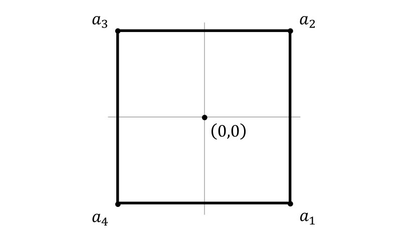
(a) $\left\{{\bf X}_{t}\right\}_{t\geq 0}$ in $[-1,1]^{2}$ square

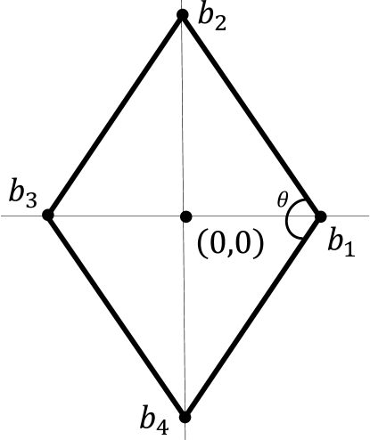
(b) $\left\{{\bf Y}_{t}\right\}_{t\geq 0}$ in $\mathbb{S}$

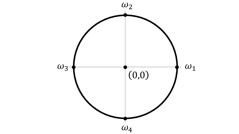
(c) $\left\{{\bf B}_{t}\right\}_{t\geq 0}$ in $\mathbb{D}$

Figure 1: Figure (a) depicts $\left\{{\bf X}_{t}\right\}_{t\geq 0}$ in the $[-1,1]^{2}$ square, Figure (b) depicts $\left\{{\bf Y}_{t}\right\}_{t\geq 0}$ in the rhombus $\mathbb{S}$, and Figure (c) depicts $\left\{{\bf B}_{t}\right\}_{t\geq 0}$ in the unit disc $\mathbb{D}$. The linear transformation ${\bf W}^{-\nicefrac{{1}}{{2}}}$ transforms the $[-1,1]^{2}$ square to $\mathbb{S}$ (Figure (a) to Figure (b)), whereas the conformal mapping $F_{\theta}$ transforms $\mathbb{D}$ to $\mathbb{S}$ (Figure (c) to Figure (b)).

To obtain the harmonic measure directly for the rhombus $\mathbb{S}$ we appeal to conformal mappings. We use the fact that the harmonic measure can be defined for any simply connected region $U$ in the plane with $0$ in its interior. More precisely, let ${\bf B}_{t}$ be standard $2$-dimensional Brownian motion started at $0$, and $\tau(U)=\inf\{t:{\bf B}_{t}\not\in U\}$ be the first time it hits the boundary of $U$. Then $\mu_{{\partial}U}$ denotes the probability measure induced by the distribution of ${\bf B}_{\tau(U)}$, and is called the harmonic measure on ${\partial}U$ (with respect to $0$). When $U$ is the unit disc centered at $0$, the harmonic measure is uniform on its boundary because Brownian motion is invariant under rotation. Then the main idea is to use conformal maps to relate harmonic measures on the different domains, namely the disc and our rhombus $\mathbb{S}$.

2.3 Conformal Mapping

Before we proceed further, it is best to transition to the language of complex numbers and identify $\mathbb{R}^{2}$ with the complex plane $\mathbb{C}$. A complex function $F:U\to V$ where $U,V\subseteq\mathbb{C}$ is conformal if it is holomorphic (i.e. complex differentiable) and its derivative $f^{\prime}(x)\neq 0$ for all $x\in U$. The key fact we use about conformal maps is that they preserve harmonic measure. Below we present this theorem from Mörters and Peres [43] specialized to our setting. In what follows, $\mathbb{D}$ will be the unit disc in $\mathbb{C}$ centered at $0$.

Theorem 5.

[43, p. 204, Theorem 7.23]. Suppose $F_{\theta}$ is a conformal map from the unit disk $\mathbb{D}$ to $\mathbb{S}$. Let $\mu_{\partial\mathbb{D}}$ and $\mu_{\partial\mathbb{S}}$ be the harmonic measures with respect to $0$. Then $\mu_{\partial\mathbb{D}}\circ F_{\theta}^{-1}=\mu_{\partial\mathbb{S}}$.

Thus the above theorem implies that in our setting, the probability that a standard Brownian motion will first hit any segment $S$ of the boundary of $\mathbb{D}$ is the same as the probability of the standard Brownian motion first hitting its image under $F_{\theta}$, i.e. $F_{\theta}(S)$ in ${\partial}\mathbb{S}$.

To complete the picture, the Schwarz-Christoffel formula gives a conformal mapping from the unit disc $\mathbb{D}$ to $\mathbb{S}$ that we utilize.

Theorem 6.

[2, Theorem 5, Section 2.2.2] Define the function $F_{\theta}(\omega)$ by

$$F_{\theta}(\omega)=\int_{s=0}^{\omega}f_{\theta}(s)ds=\int_{s=0}^{\omega}(1-s)^{-(1-\theta/\pi)}(1+s)^{-(1-\theta/\pi)}(s-i)^{-\theta/\pi}(s+i)^{-\theta/\pi}ds.$$

Then, for some real number $c>0$, $cF_{\theta}(\omega)$ is a conformal map from the unit-disk $\mathbb{D}$ to the rhombus $\mathbb{S}$.

The conformal map has some important properties which will aid us in calculating the probabilities. We collect them in the following lemma, which follows from standard properties of the Schwarz-Christoffel integral [2], and is easily verified.

Lemma 3.

The conformal map $cF_{\theta}(\omega)$ has the following properties:

1. The four points located at $\{1,i,-1,-i\}$ map to the four vertices $\{b_{1},\dots,b_{4}\}$ of the rhombus $\mathbb{S}$, respectively.

2. The origin maps to the origin.

3. The boundary of the unit-disk $\mathbb{D}$ maps to the boundary of $\mathbb{S}$. Furthermore, the points in the arc from $1$ to $i$ map to the segment $[b_{1},b_{2}]$.

Define the function $r:[0,\pi/2]\rightarrow\mathbb{R}$ as $r(\phi):=\lvert F_{\theta}(e^{i\phi})-F_{\theta}(1)\rvert$.

Lemma 4.

The probability that vertices $\{i,j\}$ are separated, given that the angle between ${\bf w}_{i}$ and ${\bf w}_{j}$ is $\theta$, is

$$\frac{2}{\pi}\int_{0}^{\pi/2}1-\frac{r(\phi)}{r(\pi/2)}d\phi$$

Proof.

Rewriting the expression in Lemma 2 in complex number notation, we have

$$\Pr[\{i,j\}\text{ separated}]=4\cdot\int_{b_{1}}^{b_{2}}1-\frac{\lvert z-b_{1}\rvert}{\lvert b_{2}-b_{1}\rvert}d\mu_{\partial\mathbb{S}}(z)=4\cdot\int_{b_{1}}^{b_{2}}1-\frac{\lvert z-cF_{\theta}(1)\rvert}{c\lvert F_{\theta}(i)-F_{\theta}(1)\rvert}d\mu_{\partial\mathbb{S}}(z).$$

Since the conformal map $F_{\theta}$ preserves the harmonic measure between the rhombus $\mathbb{S}$ and the unit-disk $\mathbb{D}$ (see Theorem 5) and by Lemma 3, the segment from $b_{1}$ to $b_{2}$ is the image of the arc from $1$ to $i$ under $cF_{\theta}$, we can rewrite the above as

$$=4\cdot\int_{0}^{\pi/2}1-\frac{\lvert cF_{\theta}(e^{i\phi})-cF_{\theta}(1)\rvert}{c\lvert F_{\theta}(i)-F_{\theta}(1)\rvert}d\mu_{\partial\mathbb{D}}(e^{i\phi}).$$

The harmonic measure $\mu_{{\partial}\mathbb{D}}$ on the unit-disk is uniform due to the rotational symmetry of Brownian motion.

$$=4\cdot\int_{0}^{\pi/2}1-\frac{\lvert cF_{\theta}(e^{i\phi})-cF_{\theta}(1)\rvert}{c\lvert F_{\theta}(i)-F_{\theta}(1)\rvert}\frac{d\phi}{2\pi}.$$

Simplifying the above, we see that the right hand side above equals

$$\frac{2}{\pi}\cdot\int_{0}^{\pi/2}1-\frac{\lvert F_{\theta}(e^{i\phi})-F(1)\rvert}{\lvert F_{\theta}(i)-F(1)\rvert}d\phi=\frac{2}{\pi}\cdot\int_{0}^{\pi/2}1-\frac{r(\phi)}{r(\pi/2)}d\phi.$$

This completes the proof. ∎

To calculate the approximation ratio exactly, we will make use of the theory of special functions. While these calculations are technical, they are not trivial. To aid the reader, we give a brief primer in Appendix B.1 and refer them to the work of Beals and Wong [18], Andrews et al. [4] for a more thorough introduction.

The proof of Theorem 4, will follow from the following key claims whose proofs appear in the appendix. Letting $a=\theta/\pi$ and $b=1-a$, we have

Claim 1.

$$r(\phi)=\frac{1}{4}\beta_{\sin^{2}\phi}(a/2,b/2)$$

when $\phi\in[0,\pi/2]$.

Claim 2.

$$4\cdot\int_{0}^{\pi/2}r(\phi)d\phi=\frac{\beta(a/2+1/2,1/2)}{2a}\cdot{}_{3}F_{2}{\left[\genfrac{.}{.}{0.0pt}{}{\frac{1+a}{2}{\mathchar 44\relax}\mskip 8.0mu\frac{1+a}{2}{\mathchar 44\relax}\mskip 8.0mu\frac{a}{2}}{\frac{a}{2}{\mathchar 44\relax}\mskip 8.0mu\frac{a}{2}+1};1\right]}$$

2.4 Asymptotic Calculation for $\theta$ close to $\pi$.

We consider the case when the angle $\theta=(1-\epsilon)\cdot\pi$ as $\epsilon\to 0$. The hyperplane-rounding algorithm separates such an edge by $\theta/\pi$, and hence has a separation probability of $1-\epsilon$. We show a similar asymptotic behaviour for the Brownian rounding algorithm, albeit with slightly worse constants. We defer the proof to the appendix.

Theorem 7.

Given an edge $\{i,j\}$ with $cos^{-1}({\bf w}_{i}^{T}{\bf w}_{j})=\theta=(1-\epsilon)\pi$, the Sticky Brownian Motion rounding will cut the edge with probability at least $1-\left(\frac{4}{\pi}\epsilon+O(\epsilon^{2})\right)$.

3 Brownian Rounding for Max-2SAT via Partial Differential Equations

In this section we use Max-2SAT as a case study for extending the Sticky Brownian Motion rounding method to other constraint satisfaction problems besides Max-Cut. In the Max-2SAT problem we are given $n$ variables $z_{1},\ldots,z_{n}$ and $m$ clauses $C_{1},\ldots,C_{m}$, where the $j$^th clause is of the form $y_{j_{1}}\vee y_{j_{2}}$ ($y_{j}$ is a literal of $z_{j}$, i.e., $z_{j}$ or $\overline{z}_{j}$). The goal is to assign to each variable $z_{i}$ a value of true or false so as to maximize the number of satisfied clauses.

3.1 Semi-definite Relaxation and Brownian Rounding Algorithm

The standard SDP relaxation used for Max-2SAT is the following:

$$\max~{}~{}~{} \sum_{j=1}^{m}\left(1-{\bf v}_{j_{1}}\cdot{\bf v}_{j_{2}}\right)$$

$$s.t.~{}~{}~{} {\bf v}_{0}\cdot{\bf v}_{0}=1$$ (1)

$${\bf v}_{0}\cdot{\bf v}_{i}={\bf v}_{i}\cdot{\bf v}_{i} \forall i=-n,\ldots,n$$ (2)

$${\bf v}_{i}\cdot{\bf v}_{-i}=0 \forall i=1,\ldots,n$$ (3)

$${\bf v}_{0}\cdot({\bf v}_{i}+{\bf v}_{-i})=1 \forall i=1,\ldots,n$$ (4)

$$1\geq{\bf v}_{0}\cdot{\bf v}_{i}+{\bf v}_{j}\cdot{\bf v}_{0}-{\bf v}_{i}\cdot{\bf v}_{j} \forall i,j=-n,\ldots,n$$ (5)

$${\bf v}_{i}\cdot{\bf v}_{0}\geq{\bf v}_{i}\cdot{\bf v}_{j} \forall i,j=-n,\ldots,n$$ (6)

$${\bf v}_{i}\cdot{\bf v}_{j}\geq 0 \forall i,j=-n.\ldots,n$$ (7)

In the above ${\bf v}_{0}$ is a unit vector that denotes the false assignment (constraint 1), whereas a zero vector denotes the true assignment. We use the standard notation that ${\bf v}_{i}$ denotes the literal $z_{i}$ and ${\bf v}_{-i}$ denotes the literal $\overline{z}_{i}$. Therefore, ${\bf v}_{i}\cdot{\bf v}_{-i}=0$ for every $i=1,\ldots.n$ (constraints 3 and 4) since $z_{i}$ needs to be either true or false. The remainder of the constraints (constraints 5, 6 and 7) are equivalent to the $\ell_{2}^{2}$ triangle inequalities over all triples of vectors that include ${\bf v}_{0}$.

When trying to generalize the Brownian rounding algorithm for Max-Cut presented in Section 2 to Max-2SAT, there is a problem: unlike Max-Cut the Max-2SAT problem is not symmetric. Specifically, for Max-Cut both $S$ and $\overline{S}$ are equivalent solutions having the same objective value. However, for Max-2SAT an assignment to the variables $z_{1}=\alpha_{1},\ldots,z_{n}=\alpha_{n}$ is not equivalent to the assignment $z_{1}=\overline{\alpha}_{1},\ldots,z_{n}=\overline{\alpha}_{n}$ (here $\alpha_{i}\in\{0,1\}$ and $\overline{\alpha}_{i}=1\oplus\alpha_{i}$). For example, if ${\bf v}_{i}\cdot{\bf v}_{0}=1$ then we would like the Brownian rounding algorithm to always assign $z_{i}$ to false. The Brownian rounding for Max-Cut cannot handle such a requirement. In order to tackle the above problem we incorporate ${\bf v}_{0}$ into both the starting point of the Brownian motion and the covariance matrix.

Let us now formally define the Brownian rounding algorithm for Max-2SAT. For simplicity of presentation denote for every $i=1,\ldots,n$ by $x_{i}$ the marginal value of $z_{i}$, formally: $x_{i}:={\bf v}_{i}\cdot{\bf v}_{0}$. Additionally, let ${\bf w}_{i}$ be the (unique) unit vector in the direction of the projection of ${\bf v}_{i}$ to the subspace orthogonal to ${\bf v}_{0}$, i.e., ${\bf w}_{i}$ satisfies ${\bf v}_{i}=x_{i}{\bf v}_{0}+\sqrt{x_{i}-x_{i}^{2}}{\bf w}_{i}$. Similarly to Max-Cut, our Sticky Brownian Motion rounding algorithm performs a random walk in $\mathbb{R}^{n}$, where the $i$^th coordinate corresponds to the variable $z_{i}$. For simplicity of presentation, the random walk is defined in $[0,1]^{n}$ as opposed to $[\pm 1]^{n}$, where $1$ denotes false and $0$ denotes true. Unlike Max-Cut, the starting point ${\bf X}_{0}$ is not the center of the cube. Instead, we use the marginals, and set $({\bf X}_{0})_{i}:=x_{i}$. The covariance matrix ${\bf W}$ is defined by ${\bf W}_{i,j}:={\bf w}_{i}\cdot{\bf w}_{j}$ for every $i,j=1,\ldots,n$, and similarly to Max-Cut, let ${\bf W}^{\nicefrac{{1}}{{2}}}$ be the principle square root of ${\bf W}$. Letting $\{{\bf B}_{t}\}_{t\geq 0}$ denote standard Brownian motion in $\mathbb{R}^{n}$, we define $\tau_{1}=\inf\{t:{\bf W}^{\nicefrac{{1}}{{2}}}{\bf B}_{t}+{\bf X}_{0}\not\in[0,1]^{n}\}$ to be the first time the process hits the boundary of $[0,1]^{n}$. Then, for all times $0\leq t\leq\tau_{1}$, the process ${\bf X}_{t}$ is defined as

$${\bf X}_{t}={\bf W}^{\nicefrac{{1}}{{2}}}{\bf B}_{t}+{\bf X}_{0}.$$

After time $\tau_{1}$, we force ${\bf X}_{t}$ to stick to the face $F_{1}$ hit at time $\tau_{1}$: i.e. if $({\bf X}_{\tau_{1}})_{i}\in\{0,1\}$, then we fix it forever, by zeroing out the $i$-th row and column of the covariance matrix of ${\bf W}$ for all future time steps. The rest of the process is defined analogously to the one for Max-Cut: whenever ${\bf X}_{t}$ hits a lower dimensional face of $[0,1]^{n}$, it is forced to stick to it until finally a vertex is reached, at which point ${\bf X}_{t}$ stops changing. We use $\tau_{i}$ for the first time that ${\bf X}_{t}$ hits a face of dimension $n-i$; then, ${\bf X}_{\tau_{n}}\in\{0,1\}^{n}$.

The output of the algorithm corresponds to the collection of the variables assigned a value of true $T\subseteq\{1,\ldots,n\}$:

$$T=\{i:\left({\bf X}_{\tau_{n}}\right)_{i}=0\},$$

whereas implicitly the collection of variables assigned a value of false are $\{i:\left({\bf X}_{\tau_{n}}\right)_{i}=1\}$.

3.2 Analysis of the Algorithm

Our goal is to analyze the expected value of the assignment produced by the Sticky Brownian Motion rounding algorithm. Similarly to previous work, we aim to give a lower bound on the probability that a fixed clause $C$ is satisfied. Unfortunately, the conformal mapping approach described in Section 2 does not seem to be easily applicable to the extended Sticky Brownian Motion rounding described above for Max-2SAT, because our calculations for Max-Cut relied heavily on the symmetry of the starting point of the random walk. We propose a different method for analyzing the Brownian rounding algorithm that is based on partial differential equations and the maximum principle. We prove analytically the following theorem which gives a guarantee on the performance of the algorithm. We also note that numerical calculations show that the algorithm in fact achieves the better approximation ratio of $0.921$ (see Section 5.1 for details).

Theorem 8.

The Sticky Brownian Motion rounding algorithm for Max-2SAT achieves an approximation of at least $0.8749$.

3.2.1 Analysis via Partial Differential Equations and Maximum Principle

As mentioned above, our analysis focuses on the probability that a single clause $C$ with variables $\{z_{i},z_{j}\}$ is satisfied. We assume the variables are not negated. This is without loss of generality as the algorithm and analysis are invariant to the sign of the variable in the clause.

For simplicity of notation we denote by $x$ the marginal value of $z_{i}$ and by $y$ the marginal value of $z_{j}$. Thus, ${\bf v}_{i}=x{\bf v}_{0}+\sqrt{x-x^{2}}{\bf w}_{i}$ and ${\bf v}_{j}=y{\bf v}_{0}+\sqrt{y-y^{2}}{\bf w}_{j}$. Projecting the random process $\{{\bf X}\}_{t\geq 0}$ on the $i$ and $j$ coordinates of the random process, we obtain a new process $\{\tilde{{\bf X}}_{t}\}_{t\geq 0}$ where $\tilde{{\bf X}}_{0}=(x,y)$. Let

$$\tilde{{\bf W}}=\begin{pmatrix}1&\cos(\theta)\\ \cos(\theta)&1\end{pmatrix},$$

where $\theta$ is the angle between ${\bf w}_{i}$ and ${\bf w}_{j}$. Then $\tilde{{\bf X}}_{t}=\tilde{{\bf X}}_{0}+\tilde{{\bf W}}^{\nicefrac{{1}}{{2}}}{\bf B}_{t}$ for all $0\leq t\leq\tau$, where $\tau=\inf\{t:\tilde{{\bf X}}_{0}+\tilde{{\bf W}}^{\nicefrac{{1}}{{2}}}{\bf B}_{t}\not\in[0,1]^{2}\}$ is the first time the process hits the boundary of the square. After time $\tau$, the process $\tilde{{\bf X}}_{t}$ performs a one-dimensional standard Brownian motion on the first side of the square it has hit, until it hits a vertex at some time $\sigma$. After time $\sigma$ the process stays fixed. Almost surely $\sigma<\infty$, and, moreover, it is easy to show that $\mathbb{E}\sigma<\infty$. We say that $\{\tilde{{\bf X}}_{t}\}_{t\geq 0}$ is absorbed at $\tilde{{\bf X}}_{\sigma}\in\{0,1\}^{2}$.

Observation 2.

The probability that the algorithm satisfies the clause $\{z_{i},z_{j}\}$ equals

$$\Pr\left[\tilde{{\bf X}}_{\sigma}\text{ is absorbed in }\{(0,0),(0,1),(1,0)\}\right].$$

We abuse notation slightly and denote $\tilde{{\bf X}_{t}}$ by ${\bf X}_{t}$ and $\tilde{{\bf W}}$ by ${\bf W}$ for the rest of the section which is aimed at analyzing the above probability. We also denote $\rho=\cos(\theta)$.

Our next step is fixing $\theta$ and analyzing the probability of satisfying the clause for all possible values of marginals $x$ and $y$. Indeed, for different $x$ and $y$ but the same $\theta$, the analysis only needs to consider the same random process with a different starting point. Observe that not all such $x,y$ are necessarily feasible for the SDP: we characterize which ones are feasible for a given $\theta$ in Lemma 7. But considering all $x,y$ allows us to handle the probability in Observation 2 analytically.

For any $0\leq x\leq 1,0\leq y\leq 1$, let $u(x,y)$ denote the probability of starting the random walk at the point $(x,y)$ and ending at one of the corners $(0,0)$, $(0,1)$ or $(1,0)$. This captures the probability of a clause being satisfied when the walk begins with marginals $(x,y)$ (and angle $\theta$). We can easily calculate this probability exactly when either $x$ or $y$ are in the set $\{0,1\}$. We obtain the following easy lemma whose proof appears in the appendix.

Lemma 5.

For $\phi(x,y)=1-xy$, we have

$$u({\bf x}) =\phi({\bf x})\text{ ~{}~{}~{}for all }{\bf x}\in{\partial}[0,1]^{2}$$ (8)

Moreover, for all ${\bf x}$ in the interior of the square $[0,1]^{2}$, $u({\bf x})=\mathbb{E}^{\bf x}[\phi({\bf X}_{\tau})]$, where $\mathbb{E}^{\bf x}$ denotes expectation with respect to starting the process at ${\bf X}_{0}={\bf x}$.

Next we use the fact that Brownian motion gives a solution to the Dirichlet boundary problem. While Brownian motion gives a solution to Laplace’s equation ([43] chapter 3), since our random process is a diffusion process, we need a slightly more general result. We state the following result from [47], specialized to our setting, that basically states that given a diffusion process in $[0,1]^{2}$ and a function $\phi$ on the boundary, the extension of the function defined on the interior by the expected value of the function at the first hitting point on the boundary is characterized by an elliptic partial differential equation.

Theorem 9 ([47] Theorem 9.2.14).

Let $D=(0,1)^{2}\subseteq\mathbb{R}^{2}$, $\mathbf{\Sigma}\in{{\mathbb{R}^{2\times 2}}}$ and let $a_{11},a_{12},a_{21},a_{22}$ be defined as follows

$$\begin{pmatrix}a_{11}&a_{12}\\ a_{21}&a_{22}\end{pmatrix}=\frac{1}{2}\mathbf{\Sigma}\mathbf{\Sigma^{\top}}.$$

For any ${\bf x}\in D$, consider the process ${\bf X}_{t}={\bf X}_{0}+\mathbf{\Sigma}{\bf B}_{t}$ where ${\bf B}_{t}$ is standard Brownian motion in $\mathbf{R}^{2}$. Let $\tau=\inf\{t:{\bf X}_{t}\not\in D\}$. Given a bounded continuous function $\phi:\partial D\rightarrow\mathbb{R}$, define the function $u:D\rightarrow\mathbb{R}$ such that

$$u({\bf x})=\mathbb{E}^{{\bf x}}\left[\phi({\bf X}_{\tau})\right],$$

where $\mathbb{E}^{{\bf x}}$ denotes the expected value when ${\bf X}_{0}={\bf x}\in\mathbb{R}^{2}$. I.e., $u({\bf x})$ is the expected value of $\phi$ when first hitting $\partial D$ conditioned on starting at point ${\bf x}$. Consider the uniformly elliptic partial differential operator $\mathcal{L}$ in $D$ defined by:

$$\mathcal{L}=\sum_{i,j=1}^{2}a_{ij}\frac{\partial^{2}}{\partial x_{i}\partial x_{j}}.$$

Then $u\in C^{2}(D)$ is the unique solution to the partial differential equation:

$$\mathcal{L}u =0 \text{ in }D$$

$$\lim_{\begin{subarray}{c}{\bf x}\rightarrow{\bf y}\\ {\bf x}\in D\end{subarray}}u({\bf x}) =\phi({\bf y}) \text{ for all }{\bf y}\in\partial D$$

We instantiate our differential equation by choosing $\mathbf{\Sigma}={\bf W}^{\nicefrac{{1}}{{2}}}$ and thus $a_{ij}$ are the entries of ${\bf W}$. It is important to note that all $a_{ij}$s are independent of the starting point ${\bf x}\in[0,1]^{2}$. Thus, we obtain that $u$ is the unique function satisfying the following partial differential equation:

$$\frac{\partial^{2}u}{\partial x^{2}}+\frac{\partial^{2}u}{\partial y^{2}}+2\rho\frac{\partial^{2}u}{\partial x\partial y} =0 \forall(x,y)\in{\operatorname{Int}}[0,1]^{2}$$

$$u(x,y) =(1-xy) \forall(x,y)\in{\partial}[0,1]^{2}$$

Above, and in the rest of the paper, we use ${\operatorname{Int}}\,D$ to denote the interior of a set $D$, and ${\partial}D$ to denote its boundary.

It remains to solve the above partial differential equation (PDE) that will allow us to calculate $u(x,y)$ and give the probability of satisfying the clause.

3.3 Maximum Principle

Finding closed form solutions general PDE’s is challenging and, there is no guarantee any solution would be expressible in terms of simple functions. However, to find a good approximation ratio, it suffices for us to find good lower-bounds on the probability of satisfying the clause. I.e. we need to give a lower bound on the function $u(x,y)$ from the previous section over those $(x,y)$ that are feasible. Since the PDE’s generated by our algorithm are elliptic (a particular kind of PDE), we will use a property of elliptic PDE’s which will allow us to produce good lower-bounds on the solution at any given point. More precisely, we use the following theorem from Gilbarg and Trudinger [28].

Let $\mathcal{L}$ denote the operator

$$\mathcal{L}:=\sum_{ij}a_{ij}\frac{\partial^{2}}{\partial_{i}\partial_{j}}$$

and we say that $\mathcal{L}$ is an elliptic operator if the coefficient matrix $A=[a_{ij}]_{i,j}$ is positive semi-definite.

We restate a version of Theorem 3.1 in Gilbarg and Trudinger [28] that shows how the maximum principle can be used to obtain lower bounds on $u(x,y)$. Here $\bar{D}$ denotes the closure of $D$.

Theorem 10 (Maximum Principle).

Let $\mathcal{L}$ be elliptic on a bounded domain $D$ and suppose $\mathcal{L}[g](x)\geq 0\;\;\forall x\in D$ for some $g\in C^{2}(D)\cap C^{0}(\bar{D})$. Then the maximum of $g$ on $D$ is achieved on $\partial D$, that is,

$$\sup_{x\in D}g(x)=\sup_{x\in\partial D}g(x)$$

Theorem 10 has the following corollary that allows us to obtain lower bounds on $u(x,y)$.

Corollary 2.

Let $\mathcal{L}$ be elliptic on a bounded domain $D$ and for some $u,g\in C^{2}(D)\cap C^{0}(\bar{D})$.

1. $\mathcal{L}[g](x)\geq\mathcal{L}[u](x)\quad\forall x\in D$

2. $g(x)\leq u(x)\quad\forall x\in\partial D$

then $g(x)\leq u(x)\forall x\in D$.

We refer the reader to [28] for a formal proof. Thus, it is enough to construct candidate functions $g:[0,1]^{2}\rightarrow\mathbb{R}$ such that

$$\frac{\partial^{2}g}{\partial x^{2}}+\frac{\partial^{2}g}{\partial y^{2}}+2\rho\frac{\partial^{2}g}{\partial x\partial y} \geq 0 \forall(x,y)\in{\operatorname{Int}}[0,1]^{2}$$ (9)

$$g(x,y) \leq(1-xy) \forall(x,y)\in\partial[0,1]^{2}$$ (10)

Then we obtain that $g(x,y)\leq u(x,y)$ for all $(x,y)\in[0,1]^{2}$. In what follows we construct many different such function each of which works for a different range of the parameter $\theta$ (equivalently, $\rho$).

3.4 Candidate Functions for Maximum Principle

We now construct feasible candidates to the maximum principle as described in Corollary 2. We define the following functions:

1. $g_{1}(x,y)=1-xy-\cos(\theta)\sqrt{x-x^{2}}\sqrt{y-y^{2}}$.

2. $g_{2}(x,y)=1-xy-2\cos(\theta)(x-x^{2})(y-y^{2})$.

3. $g_{3}(x,y)=1-xy-\frac{1}{2}(1+5\cos(\theta))(x-x^{2})(y-y^{2})(x+y)(2-x-y)$.

The following lemma shows that the above functions satisfy the conditions required for the application of the maximum principle (its proof appears in the appendix).

Lemma 6.

Each of $g_{1},g_{2},g_{3}$ satisfies the boundary conditions, i.e. $g_{i}(x,y)=u(x,y)$ for all $x,y\in\partial[0,1]^{2}$ and for all values $\theta$. Moreover, we have the following for each $(x,y)\in[0,1]^{2}$:

1. If $1\geq\cos(\theta)\geq 0$, then $\mathcal{L}g_{1}\geq 0$.

2. If $0\geq\cos(\theta)\geq-\frac{1}{2}$, then $\mathcal{L}g_{2}\geq 0$.

3. If $-\frac{1}{2}\geq\cos(\theta)\geq-1$, then $\mathcal{L}g_{3}\geq 0$.

While some of these proofs are based on simple inequalities, proving others requires us to use sum of squares expressions. For example, to show $\mathcal{L}g_{3}\geq 0$, we consider $\mathcal{L}g_{3}=p(x,y,\cos(\theta))$ as a polynomial in $x,y$ and $\cos(\theta)$. Replacing $z=\cos(\theta)$, our aim is to show $p(x,y,z)\geq 0$ if $0\leq x,y\leq 1$ and $-1\leq z\leq-\frac{1}{2}$. Equivalently, we need to show $p(x,y,z)\geq 0$ whenever $r_{1}(x,y,z):=x-x^{2}\geq 0$, $r_{2}(x,y,z):=y-y^{2}\geq 0$ and $r_{3}(x,y,z):=-(z+\frac{1}{2})\geq 0$ and $r_{4}(x,y,z):=(z+1)\geq 0$. We show this by obtaining polynomials $q_{i}(x,y,z)$ for $i=0,1,2,3,4$ such that each $q_{i}$ is a sum of squares polynomial of fixed degree and we have

$$p(x,y,z)=q_{0}(x,y,z)+\sum_{i=1}^{4}q_{i}(x,y,z)r_{i}(x,y,z).$$

Observe that the above polynomial equality proves the desired result by evaluating the RHS for every $0\leq x,y\leq 1$ and $-\nicefrac{{1}}{{2}}\geq z\geq-1$. Clearly, the RHS is non-negative: each $q_{i}$ is non-negative since it is a sum of squares and each $r_{i}$ is non-negative in the region we care about, by construction. We mention that we obtain these proofs via solving a semi-definite program of fixed degree (at most 6) for each of the $q_{i}$ polynomials (missing details appear in the appendix).

Let us now focus on the approximation guarantee that can be proved using the above functions $g_{1}$, $g_{2}$, and $g_{3}$. The following lemma compares the lower bounds on the probability of satisfying a clause, as given by $g_{1}$, $g_{2}$, and $g_{3}$, to the SDP objective. Recall that the contribution of any clause with marginals $x$ and $y$ and angle $\theta$ to the SDP’s objective is given by: $1-xy-\cos(\theta)\sqrt{x-x^{2}}\sqrt{y-y^{2}}$. We denote this contribution by $\textsc{SDP}(x,y,\theta)$. It is important to note that not all triples $(x,y,\theta)$ are feasible (recall that $\theta$ is the angle between ${\bf w}_{i}$ and ${\bf w}_{j}$), due to the triangle inequalities in the SDP. This is summarized in the following lemma.

Lemma 7.

Let $x,y,\theta$ be as defined by a feasible pair of vectors $v_{i}$ and $v_{j}$. Then they must satisfy the following constraints:

1. $0\leq x\leq 1,0\leq y\leq 1,0\leq\theta\leq\pi$.

2. $\cos(\theta)\geq-\sqrt{\frac{xy}{(1-x)(1-y)}}$.

3. $\cos(\theta)\geq-\sqrt{\frac{(1-x)(1-y)}{xy}}$.

Finally, we prove the following lemma which proves an approximation guarantee of 0.8749 for Max-2SAT via the PDE and the maximum principle approach. As before, these proofs rely on explicitly obtaining sum of squares proofs as discussed above. We remark that these proofs essentially aim to obtain $\frac{7}{8}=0.875$-approximation but errors of the order $10^{-5}$ allow us to obtain a slightly worse bound using this methods. The details appear in the appendix.

Lemma 8.

Consider any feasible triple $(x,y,\theta)$ satisfying the condition in Lemma 7. We have the following.

1. If $1\geq\cos(\theta)\geq 0$, then $g_{1}(x,y)\geq 1\cdot\textsc{SDP}(x,y,\theta)$.

2. If $0\geq\cos(\theta)\geq-\frac{1}{2}$, then $g_{2}(x,y)\geq$0.8749$\cdot\textsc{SDP}(x,y,\theta)$.

3. If $-\frac{1}{2}\geq\cos(\theta)\geq-1$, then $g_{3}(x,y)\geq$0.8749$\cdot\textsc{SDP}(x,y,\theta)$.

4 Max-Cut with Side Constraints (Max-Cut-SC)

In this section we describe how to apply the Sticky Brownian Motion rounding and the framework of Raghavendra and Tan [50] to the Max-Cut-SC problem in order to give a bi-criteria approximation algorithm whose running time is non-trivial even when the the number of constraints is large.

4.1 Problem Definition and Basics

Let us recall the relevant notation and definitions. An instance of the Max-Cut-SC problem is given by an $n$-vertex graph $G=(V,E)$ with edge weights $a:E\to\mathbb{R}_{+}$, as well as a collection ${\cal F}=\{F_{1},\ldots,F_{k}\}$ of subsets of $V$, and cardinality bounds $b_{1},\ldots,b_{k}\in\mathbb{N}$. For ease of notation, we will assume that $V=\{1,\ldots,n\}$. Moreover, we denote the total edge weight by $a(E)=\sum_{e\in E}{a(e)}$. The goal in the Max-Cut-SC problem is to find a subset $S\subset V$ that maximizes the weight $a(\delta(S))$ of edges crossing the cut $(S,V\setminus S)$, subject to having $|S\cap F_{i}|=b_{i}$ for all $i\in[k]$. These cardinality constraints may not be simultaneously satisfiable, and moreover, when $k$ grows with $n$, checking satisfiability is $\mathsf{NP}$-hard [23]. For these reasons, we allow for approximately feasible solutions. We will say that a set of vertices $S\subseteq V$ is an $(\alpha,\varepsilon)$-approximation to the Max-Cut-SC problem if $\bigl{|}|S\cap F_{i}|-b_{i}\bigr{|}\leq\varepsilon n$ for all $i\in[k]$, and $a(\delta(S))\geq\alpha\cdot a(\delta(T))$ for all $T\subset V$ such that $|T\cap F_{i}|=b_{i}\$ for all $i\in[k]$. In the remainder of this section we assume that the instance given by $G$, ${\cal F}$, and $b$ is satisfiable, i.e. that there exists a set of vertices $T$ such that $|T\cap F_{i}|=b_{i}\$ for all $i\in[k]$. Our algorithm may fail if this assumption is not satisfied. If this happens, then the algorithm will certify that the instance was not satisfiable.

We start with a simple baseline approximation algorithm, based on independent rounding. The algorithm outputs an approximately feasible solution which cuts a constant fraction of the total edge weight. For this reason, it achieves a good bi-criteria approximation when the value of the optimal solution OPT is much smaller than $\varepsilon a(E)$. This allows us to focus on the case in which OPT is bigger than $\varepsilon a(E)$ for our main rounding algorithm. The proof of the lemma, which follows from standard arguments, appears in the appendix.

Lemma 9.

Suppose that $n\geq\frac{2\ln(8k/\varepsilon)}{\varepsilon^{2}}$ and $\varepsilon\leq\frac{1}{2}$. There exists a polynomial time algorithm that on input a satisfiable instance $G=(V,E)$, ${\cal F}$, and $b_{1},\ldots,b_{k}$, as defined above, outputs a set $S\subseteq V$ such that, with high probability, $a(\delta(S))\geq\frac{\varepsilon}{2}a(E)$, and $\bigl{|}|S\cap F_{i}|-b_{i}\bigr{|}\leq\varepsilon n$ for all $i\in[k]$.

4.2 Sum of Squares Relaxation

Our main approximation algorithm is based on a semidefinite relaxation, and the sticky Brownian motion. Let us suppose that we are given the optimal objective value OPT of a feasible solution: this assumption can be removed by doing binary search for OPT. We can then model the problem of finding an optimal feasible solution by the quadratic program

$$\sum_{e=(i,j)\in E}{a(e)(x_{i}-x_{j})^{2}}\geq\textsc{OPT}$$

s.t. $$~{}~{}~{}~{}\sum_{j\in F_{i}}{x_{j}}=b_{i} \forall i=1,\ldots,k$$

$$x_{j}(1-x_{j})=0 \forall j=1,\ldots,k$$

Let us denote this quadratic feasibility problem by $Q$. The Sum of Squares (Lasserre) hierarchy gives a semidefinite program that relaxes $Q$. We denote by $\mathrm{SoS}_{\ell}(Q)$ the solutions to the level-$\ell$ Sum of Squares relaxations of $Q$. Any solution in $\mathrm{SoS}_{\ell}(Q)$ can be represented as a collection of vectors $\mathcal{V}=\{{\bf v}_{S}:S\subseteq[n],0\leq|S|\leq\ell\}$. To avoid overly cluttered notation, we write ${\bf v}_{i}$ for ${\bf v}_{\{i\}}$; we also write ${\bf v}_{0}$ for ${\bf v}_{\emptyset}$. We need the following properties of $\mathcal{V}$, valid as long as $\ell\geq 2$.

1. ${\bf v}_{0}\cdot{\bf v}_{0}=1$.

2. ${\bf v}_{S}\cdot{\bf v}_{T}={\bf v}_{S^{\prime}}\cdot{\bf v}_{T^{\prime}}$ for any $S,S^{\prime},T,T^{\prime}$ such that $S\cup T=S^{\prime}\cup T^{\prime}$ and $|S\cup T|\leq k$. In particular, ${\bf v}_{i}\cdot{\bf v}_{i}={\bf v}_{i}\cdot{\bf v}_{0}$ for any $i$.

3. For any $i$ and $j$ the following inequalities hold:

   $$1\geq{\bf v}_{0}\cdot{\bf v}_{i}+{\bf v}_{j}\cdot{\bf v}_{0}-{\bf v}_{i}\cdot{\bf v}_{j}$$ (11)

   $${\bf v}_{i}\cdot{\bf v}_{0}\geq{\bf v}_{i}\cdot{\bf v}_{j}$$ (12)

   $${\bf v}_{i}\cdot{\bf v}_{j}\geq 0$$ (13)

4. $\sum_{e=(i,j)\in E}{a(e)\|{\bf v}_{i}-{\bf v}_{j}\|^{2}}\geq\textsc{OPT}$

5. For any $i$, there exist two solutions $\mathcal{V}^{i\to 0}$ and $\mathcal{V}^{i\to 1}$ in $\mathrm{SoS}_{\ell-1}(Q)$ such that, if we denote the vectors in $\mathcal{V}^{i\to 0}$ by ${\bf v}_{S}^{0}$, and the vectors in $\mathcal{V}^{i\to 1}$ by ${\bf v}_{S}^{1}$, we have

   $${\bf v}_{S}\cdot{\bf v}_{0}=(1-{\bf v}_{i}\cdot{\bf v}_{0}){\bf v}^{0}_{S}\cdot{\bf v}^{0}_{0}+({\bf v}_{i}\cdot{\bf v}_{0}){\bf v}^{1}_{S}\cdot{\bf v}^{1}_{0}.$$

Moreover, a solution $\mathcal{V}\in\mathrm{SoS}_{\ell}$ can be computed in time polynomial in $n^{\ell}$.

Intuitively, we think of $\mathcal{V}$ as describing a pseudo-distribution over solutions to $Q$, and we interpret ${\bf v}_{S}\cdot{\bf v}_{T}$ as the pseudo-probability that all variables in $S\cup T$ are set to one, or, equivalently, as the pseudo-expectation of $\prod_{i\in S\cup T}x_{i}$. Usually we cannot expect that there is any true distribution giving these probabilities. Nevertheless, the pseudo-probabilities and pseudo-expectations satisfy some of the properties of actual probabilities. For example, the transformation from $\mathcal{V}$ to $\mathcal{V}^{i\to b}$ corresponds to conditioning $x_{i}$ to $b$.

We will denote by $x_{S}={\bf v}_{S}\cdot{\bf v}_{0}$ the marginal value of set $S$. In particular, we will work with the single-variable marginals $x_{i}=x_{\{i\}}={\bf v}_{i}\cdot{\bf v}_{0}$, and will denote ${\bf x}=(x_{1},\ldots,x_{n})$. As before, it will be convenient to work with the component of ${\bf v}_{i}$ which is orthogonal to ${\bf v}_{0}$. We define $\widetilde{{\bf w}}_{i}={\bf v}_{i}-x_{i}{\bf v}_{0}$, and ${\bf w}_{i}=\frac{1}{\|\widetilde{{\bf w}}_{i}\|}\widetilde{{\bf w}}_{i}$. Note that, by the Pythagorean theorem, $\|\widetilde{{\bf w}}_{i}\|^{2}=x_{i}-x^{2}_{i}$, and ${\bf v}_{i}=x_{i}{\bf v}_{0}+\sqrt{x_{i}-x_{i}^{2}}{\bf w}_{i}$. We define the matrices $\widetilde{{\bf W}}$ and ${\bf W}$ by $\widetilde{{\bf W}}_{i,j}:=\widetilde{{\bf w}}_{i}\cdot\widetilde{{\bf w}}_{j}$ and ${\bf W}_{i,j}:={\bf w}_{i}\cdot{\bf w}_{j}$. We can think of $\widetilde{{\bf W}}$ as the covariance matrix of the pseudodistribution corresponding to the SDP solution. The following lemma, due to Barak, Raghavendra, and Steurer [17], and, independently, to Guruswami and Sinop [32], shows that any pseudodistribution can be conditioned so that the covariances are small on average.

Lemma 10.

For any $\varepsilon_{0}\leq 1$, and any $\mathcal{V}\in\mathrm{SoS}_{\ell}(Q)$, where $\ell\geq\frac{1}{\varepsilon_{0}^{4}}+2$, there exists an efficiently computable $\mathcal{V}^{\prime}\in\mathrm{SoS}_{\ell-1/\varepsilon_{0}^{4}}(Q)$, such that

$$\sum_{i=1}^{n}\sum_{j=1}^{n}{\widetilde{{\bf W}}_{i,j}^{2}}\leq\varepsilon_{0}^{4}n^{2}.$$ (14)

In particular, $\mathcal{V}^{\prime}$ can be computed by conditioning $\mathcal{V}$ on $\frac{1}{\varepsilon_{0}^{4}}$ variables.

4.3 Rounding Algorithm

For our algorithm, we first solve a semidefinite program to compute a solution in $\mathrm{SoS}_{\ell}(Q)$, to which we apply Lemma 10 with parameter $\varepsilon_{0}$, which we will choose later. In order to be able to apply the lemma, we choose $\ell=\left\lceil\frac{1}{\varepsilon_{0}^{4}}\right\rceil+2$. The rounding algorithm itself is similar to the one we used for Max-2SAT. We perform a Sticky Brownian Motion with initial covariance ${\bf W}$, starting at the initial point ${\bf X}_{0}={\bf x}$, i.e. at the marginals given by the SDP solution. As variables hit $0$ or $1$, we freeze them, and delete the corresponding row and column of the covariance matrix. The main difference from the Max-2SAT rounding is that we stop the process at time $\tau$, where $\tau$ is another parameter that we will choose later. Then, independently for each $i=1,\ldots,n$, we include vertex $i$ in the final solution $S$ with probability $({\bf X}_{\tau})_{i}$, and output $S$.

The key property of this rounding that allows us to handle a large number of global constraints is that, for any $F_{i}\in{\cal F}$, the value $\sum_{j\in F_{i}}({\bf X}_{\tau})_{j}$ that the fractional solution assigns to the set $F_{i}$ satisfies a sub-Gaussian concentration bound around $b_{i}$. Note that $\sum_{j\in F_{i}}({\bf X}_{t})_{j}$ is a martingale with expectation equal to $b_{i}$. Moreover, by Lemma 10, the entries of the covariance matrix $\widetilde{{\bf W}}$ are small on average, which allows us to also bound the entries of the covariance matrix ${\bf W}$, and, as a consequence, bound how fast the variance of the martingale increases with time. The reason we stop the walk at time $\tau$ is to make sure the variance doesn’t grow too large: this freedom, allowed by the Sticky Brownian Motion rounding, is important for our analysis. The variance bound then implies the sub-Gaussian concentration of $\sum_{j\in F_{i}}({\bf X}_{\tau})_{j}$ around its mean $b_{i}$, and using this concentration we can show that no constraint is violated by too much. This argument crucially uses the fact that our rounding is a random walk with small increments, and we do not expect similarly strong concentration results for the random hyperplane rounding or its variants.

The analysis of the objective function, as usual, reduces to analyzing the probability that we cut an edge. However, because we start the Sticky Brownian Motion at ${\bf x}$, which may not be equal to $\mathbf{0}$, our analysis from Section 2 is not sufficient. Instead, we use the PDE based analysis from Section 3, which easily extends to the Max-Cut objective. One detail to take care of is that, because we stop the walk early, edges incident on vertices that have not reached $0$ or $1$ by time $\tau$ may be cut with much smaller probability than their contribution to the SDP objective. To deal with this, we choose the time $\tau$ when we stop the walk large enough, so that any vertex has probability at least $1-\mathrm{poly}(\varepsilon)$ to have reached $\{0,1\}$ by time $\tau$. We show that this happens for $\tau=\Theta(\log(1/\varepsilon))$. This value of $\tau$ is small enough so that we can usefully bound the variance of $\sum_{j\in F_{i}}({\bf X}_{\tau})_{i}$ and prove the sub-Gaussian concentration we mentioned above.

Let us recall some notation that will be useful in our analysis. We will use $\tau_{i}$ for the first time $t$ that ${\bf X}_{t}$ hits a face of $[0,1]^{n}$ of dimension $n-i$; then, ${\bf X}_{\tau_{n}}\in\{0,1\}^{n}$. We also use ${\bf W}_{t}$ for the covariance used at time step $t$, which is equal to ${\bf W}$ with rows and columns indexed by $\{i:({\bf X}_{t})_{i}\in\{0,1\}\}$ zeroed out.

As discussed, our analysis relies on a martingale concentration inequality, and the following lemma, which is proved with the methods we used above for the Max-2SAT problem. A proof sketch can be found in the appendix.

Lemma 11.

For the SDP solution $\mathcal{V}$ and the Sticky Brownian Motion ${\bf X}_{t}$ described above, and for any pair $\{i,j\}$ of vertices

$$\Pr[({\bf X}_{\tau_{n}})_{i}\neq({\bf X}_{\tau_{n}})_{j}]\geq 0.843\cdot\|{\bf v}_{i}-{\bf v}_{j}\|^{2}.$$

The next lemma shows that the probability that any coordinate is fixed by time $t$ drops exponentially with $t$. We use this fact to argue that by time $\tau=\Theta(\log(1/\varepsilon))$ the endpoints of any edge have probability at least $1-\mathrm{poly}(\varepsilon)$ to be fixed, and, therefore, edges are cut with approximately the same probability as if we didn’t stop the random walk early, which allows us to use Lemma 11. The proof of this lemma, which is likely well-known, appears in the appendix.

Lemma 12.

For any $i$, and any integer $t\geq 0$, $\Pr[\forall s\leq t:0<({\bf X}_{s})_{i}<1]<4^{-t}$.

The following concentration inequality is our other key lemma. The statement is complicated by the technical issue that the concentration properties of the random walk depend on the covariance matrix ${\bf W}$, while Lemma 10 bounds the entries of $\widetilde{{\bf W}}$. When $x_{i}(1-x_{i})$ or $x_{j}(1-x_{j})$ is small, $\widetilde{{\bf W}}_{i,j}$ can be much smaller than ${\bf W}_{i,j}$. Because of this, we only prove our concentration bound for sets of vertices $i$ for which $x_{i}(1-x_{i})$ is sufficiently large. For those $i$ for which $x_{i}(1-x_{i})$ is small, we will instead use the fact that such $x_{i}$ are already nearly integral to prove a simpler concentration bound.

Lemma 13.

Let $\varepsilon_{0},\varepsilon_{1}\in[0,1]$, and $n\geq\frac{\varepsilon_{1}}{8\tau\varepsilon_{0}^{2}}$. Define $V_{>\varepsilon_{1}}=\{i:2x_{i}(1-x_{i})>\varepsilon_{1}\}$. For any set $F\subseteq V_{>\varepsilon_{1}}$, and any $t\geq 0$, the random set $S$ output by the rounding algorithm satisfies

$$\Pr\left[\Bigl{|}|F\cap S|-\sum_{i\in F}{x_{i}}\Bigr{|}\geq t\varepsilon_{0}n\right]\leq 4\exp\left(-\frac{\varepsilon_{1}t^{2}}{4\tau}\right).$$

We give the proof of Lemma 13 after we finish the proof of Theorem 3, restated below for convenience.

See 3

Proof.

The algorithm outputs either the set $S$ output by the Sticky Brownian Rounding described above, or the one guaranteed by Lemma 9, depending on which one achieves a cut of larger total weight. If $\textsc{OPT}\leq\frac{\varepsilon}{2}a(E)$, then Lemma 9 achieves the approximation we are aiming for. Therefore, for the rest of the proof, we may assume that $\textsc{OPT}\geq\frac{\varepsilon}{2}a(E)$, and that the algorithm outputs the set $S$ computed by the Sticky Brownian Rounding. Then, it is enough to guarantee that, with high probability,

$$a(\delta(S))\geq 0.843\cdot\textsc{OPT}-\frac{\varepsilon^{2}}{2}a(E).$$ (15)

Let us set $\varepsilon_{1}=\varepsilon^{2}\varepsilon_{0}$, and define, as above, $V_{>\varepsilon_{1}}=\{i:2x_{i}(1-x_{i})>\varepsilon_{1}\}$ and let $V_{\leq\varepsilon_{1}}=\{i:2x_{i}(1-x_{i})\leq\varepsilon_{1}\}$. Let ${\bf Y}$ be the indicator vector of the set $S$ output by the algorithm. Observe that, for each $i$, since ${\bf Y}_{i}$ is a Bernoulli random variable with expectation $x_{i}$, we have $\mathbb{E}\left[\sum_{i\in V_{\leq\varepsilon_{1}}}{|{\bf Y}_{i}-x_{i}|}\right]\leq\varepsilon_{1}n$, and, therefore,

$$\Pr\left[\sum_{i\in V_{\leq\varepsilon_{1}}}{|{\bf Y}_{i}-x_{i}|}\geq 16\varepsilon_{0}n\right]\leq\frac{\varepsilon^{2}}{16}.$$

Then, for any $F_{i}\in{\cal F}$, by Lemma 13 applied to $F_{i}\cap V_{>\varepsilon_{1}}$, we have

$$\Pr\left[\bigl{|}|F_{i}\cap V_{>\varepsilon_{1}}\cap S|-\sum_{i\in F\cap V_{>\varepsilon_{1}}}{x_{i}}\bigr{|}\geq\sqrt{\frac{4\tau}{\varepsilon_{1}}\ln\frac{32k}{\varepsilon^{2}}}\varepsilon_{0}n\right]\leq\frac{\varepsilon^{2}}{16k}.$$

Therefore, with probability at least $1-\frac{\varepsilon^{2}}{8}$, for all $i\in[k]$ we have

$$\left||F_{i}\cap S|-\sum_{i\in F}{x_{i}}\right| \leq\left||F_{i}\cap V_{\leq\varepsilon_{0}}\cap S|-\sum_{i\in F\cap V_{\leq\varepsilon_{0}}}{x_{i}}\right|+\left||F_{i}\cap V_{>\varepsilon_{0}}\cap S|-\sum_{i\in F\cap V_{>\varepsilon_{0}}}{x_{i}}\right|$$

$$\leq\sum_{i\in F\cap V_{\leq\varepsilon_{0}}}{|{\bf Y}_{i}-x_{i}|}+\left||F_{i}\cap V_{>\varepsilon_{0}}\cap S|-\sum_{i\in F\cap V_{>\varepsilon_{0}}}{x_{i}}\right|$$

$$\leq\left(16+\sqrt{\frac{4\tau}{\varepsilon^{2}\varepsilon_{0}}\ln\frac{32k}{\varepsilon^{2}}}\right)\varepsilon_{0}n.$$

This means that, with probability at least $1-\frac{\varepsilon^{2}}{8}$, $S$ satisfies all the constraints up to additive error $\varepsilon n$, as long as

$$\varepsilon_{0}\leq\min\Biggl{\{}\frac{\varepsilon}{32},\frac{\varepsilon^{4}}{4\sqrt{\tau\ln\frac{32k}{\varepsilon^{2}}}}\Biggr{\}}.$$

It remains to argue about the objective function. For $\tau\geq\log_{2}\frac{2\sqrt{2}}{\varepsilon}$, Lemma 12 implies that, for any vertex $i$, $\Pr[({\bf X}_{\tau})_{i}\not\in\{0,1\}]\leq 4^{-\tau}\leq\frac{\varepsilon^{2}}{8}$. By Lemma 11, any pair of vertices $\{i,j\}$ is separated with probability

$$\Pr[({\bf X}_{\tau_{n}})_{i}\neq({\bf X}_{\tau_{n}})_{j}]\geq 0.843\cdot\|{\bf v}_{i}-{\bf v}_{j}\|^{2},$$

where we recall that, for edge $e=(i,j)$, $a(e)\|{\bf v}_{i}-{\bf v}_{j}\|^{2}$ is the contribution of $e$ to the objective value. Then,

$$\Pr[({\bf X}_{\tau})_{i}\neq({\bf X}_{\tau})_{j}] \geq\Pr[({\bf X}_{\tau_{n}})_{i}\neq({\bf X}_{\tau_{n}})_{j},({\bf X}_{\tau})_{i}=({\bf X}_{\tau_{n}})_{i},({\bf X}_{\tau})_{j}=({\bf X}_{\tau_{n}})_{j}]$$

$$=\Pr[({\bf X}_{\tau_{n}})_{i}\neq({\bf X}_{\tau_{n}})_{j},({\bf X}_{\tau})_{i}\in\{0,1\},({\bf X}_{\tau})_{j}\in\{0,1\}]$$

$$\geq\Pr[({\bf X}_{\tau_{n}})_{i}\neq({\bf X}_{\tau_{n}})_{j}]-\frac{\varepsilon^{2}}{4}$$

$$\geq 0.843\cdot\|{\bf v}_{i}-{\bf v}_{j}\|_{2}^{2}-\frac{\varepsilon^{2}}{4}.$$

Therefore, $\mathbb{E}[a(\delta(S))]\geq 0.843\cdot\textsc{OPT}-\frac{\varepsilon^{2}}{4}a(E)$. By Markov’s inequality applied to $a(E)-a(\delta(S))$,

$$\Pr\Bigl{[}a(\delta(S)]<0.843\cdot\textsc{OPT}-\frac{\varepsilon^{2}}{2}a(E)\Bigr{]}<\frac{1+\frac{\varepsilon^{2}}{4}}{1+\frac{\varepsilon^{2}}{2}}<1-\frac{\varepsilon^{2}}{5}.$$

In conclusion, we have that with probability at least $\frac{3}{40}\varepsilon^{2}$, (15) is satisfied, and all global constraints are satisfied up to an additive error of $\varepsilon n$. The probability can be made arbitrarily close to $1$ by repeating the entire algorithm $O(\varepsilon^{-2})$ times. To complete the proof of the theorem, we can verify that the running time is dominated by the time required to find a solution in $\mathrm{SoS}_{\ell}(Q)$, which is polynomial in $n^{\ell}$, where $\ell=O(\varepsilon_{0}^{-4})=\mathrm{poly}(\log(k)/\varepsilon)$. ∎

We finish this section with the proof of Lemma 13

Proof of Lemma 13.

Since each $i$ is included in $S$ independently with probability $({\bf X}_{\tau})_{i}$, by Hoeffding’s inequality we have

$$\Pr\left[\Bigl{|}|F\cap S|-\sum_{i\in F}{({\bf X}_{\tau})_{i}}\Bigr{|}\geq t\varepsilon_{1}n\right]\leq 2e^{-2\varepsilon_{1}^{2}t^{2}n}\leq 2\exp\left(-\frac{\varepsilon_{1}t^{2}}{4\tau}\right),$$

where the final inequality follows by our assumption on $n$. Therefore, it is enough to establish

$$\Pr\left[\Bigl{|}\sum_{i\in F}{({\bf X}_{\tau})_{i}-x_{i}}\Bigr{|}\geq t\varepsilon_{1}n\right]\leq 2\exp\left(-\frac{\varepsilon_{1}t^{2}}{4\tau}\right).$$ (16)

Suppose ${\bf y}\in\{0,1\}^{n}$ is the indicator vector of $F$ so that

$${\bf y}^{\top}({\bf X}_{\tau}-{\bf X}_{0})={\bf y}^{\top}({\bf X}_{\tau}-{\bf x})=\sum_{i\in F}{(({\bf X}_{\tau})_{i}-x_{i})}.$$

A standard calculation using Itô’s lemma (see Exercise 4.4. in [47]) shows that, for any $\lambda\geq 0$, the random process

$$Y_{t}=\exp\left(\lambda{\bf y}^{\top}({\bf X}_{t}-{\bf x})-\frac{\lambda^{2}}{2}\int_{0}^{t}({\bf y}^{\top}{\bf W}_{s}{\bf y})ds\right)$$

is a martingale with starting state $Y_{0}=1$. Since, for any $s$, ${\bf W}_{s}$ equals ${\bf W}$ with some rows and columns zeroed out, we have that ${\bf W}-{\bf W}_{s}$ is positive semidefinite, and ${\bf y}^{\top}{\bf W}_{s}{\bf y}\leq{\bf y}^{\top}{\bf W}{\bf y}$. Therefore,

$$\mathbb{E}\left[\exp\Bigl{(}\lambda{\bf y}^{\top}({\bf X}_{\tau}-{\bf x})-t\frac{\lambda^{2}}{2}{\bf y}^{\top}{\bf W}{\bf y}\Bigr{)}\right]\leq\mathbb{E}[Y_{\tau}]=1.$$

Rearranging, this gives us that, for all $\lambda\geq 0$,

$$\mathbb{E}[e^{\lambda{\bf y}^{\top}({\bf X}_{\tau}-{\bf x})}]\leq\mathbb{E}[e^{\tau\lambda^{2}{\bf y}^{\top}{\bf W}{\bf y}/2}]\leq e^{\tau\lambda^{2}{\bf y}^{\top}{\bf W}{\bf y}/2}.$$ (17)

We can bound ${\bf y}^{\top}{\bf W}{\bf y}$ using Cauchy-Schwarz, the assumption that $2x_{i}(1-x_{i})>\varepsilon_{1}$ for all $i\in F$, and (14):

$${\bf y}^{\top}{\bf W}{\bf y} =\sum_{i\in F}\sum_{j\in F}{{\bf W}_{i,j}}$$

$$\leq|F|\left(\sum_{i\in F}\sum_{j\in F}{{\bf W}_{i,j}^{2}}\right)^{1/2}$$

$$=|F|\left(\sum_{i\in F}\sum_{j\in F}{\frac{\widetilde{{\bf W}}_{i,j}^{2}}{x_{i}x_{j}(1-x_{i})(1-x_{j})}}\right)^{1/2}$$

$$<\frac{2n}{\varepsilon_{1}}\left(\sum_{i\in F}\sum_{j\in F}{\widetilde{{\bf W}}_{i,j}^{2}}\right)^{1/2}$$

$$\leq\frac{2\varepsilon_{0}^{2}n^{2}}{\varepsilon_{1}}.$$

Plugging back into (17), we get $\mathbb{E}[e^{\lambda{\bf y}^{\top}({\bf X}_{\tau}-{\bf x})}]\leq e^{\tau\lambda^{2}\varepsilon_{0}^{2}n^{2}/\varepsilon_{1}}$. The standard exponential moment argument then implies (16). ∎

5 Extensions of the Brownian Rounding

In this section, we consider two extensions of the Brownian rounding algorithm. We also present numerical results for these variants showing improved performance over the sticky Brownian Rounding analyzed in previous sections.

5.1 Brownian Rounding with Slowdown

As noted in section 2, the Sticky Brownian rounding algorithm does not achieve the optimal value for the Max-Cut problem. A natural question is to ask if we can modify the algorithm to achieve the optimal constant. In this section, we will show that a simple modification achieves this ratio up to at least three decimals. Our results are computer-assisted as we solve partial differential equations using finite element methods. These improvement indicate that variants of the Brownian Rounding approach offer a direction to obtain optimal SDP rounding algorithms for Max-Cut problem as well as other CSP problems.

In the sticky Brownian motion, the covariance matrix $W_{t}$ is a constant, until some vertex’s marginals $({\bf X}_{t})_{i}$ becomes $\pm 1$. At that point, we abruptly zero the $i^{th}$ row and column. In this section, we analyze the algorithm where we gradually dampen the step size of the Brownian motion as it approaches the boundary of the hypercube, until it becomes $0$ at the boundary. We call this process a “Sticky Brownian Motion with Slowdown.”

Let $({\bf X}_{t})_{i}$ denote the marginal value of vertex $i$ at time $t$. Initially $({\bf X}_{0})_{i}=0$. First, we describe the discrete algorithm which will provide intuition but will also be useful to those uncomfortable with Brownian motion and diffusion processes. At each time step, we will take a step whose length is scaled by a factor of $(1-({\bf X}_{t})_{i}^{2})^{\alpha}$ for some constant $\alpha$. In particular, the marginals will evolve according to the equation:

$$({\bf X}_{t+dt})_{i} =({\bf X}_{t})_{i}+(1-({\bf X}_{t})_{i})^{2})^{\alpha/2}\cdot\big{(}{\bf w}_{i}\cdot\mathbf{G}_{t}\big{)}\cdot\sqrt{dt}.$$ (18)

where $\mathbf{G}_{t}$ is distributed according to an $n$-dimensional Gaussian and $dt$ is a small discrete step by which we advance the time variable. When ${\bf X}_{t}$ is sufficiently close to $-1$ or $+1$, we round it to the nearest one of the two: from then on it will stay fixed because of the definition of the process, i.e. we will have $({\bf X}_{s})_{i}=({\bf X}_{t})_{i}$ for all $s>t$.

More formally, ${\bf X}_{t}$ is defined as an Itô diffusion process which satisfies the stochastic differential equation

$$d{\bf X}_{t}=\mathbf{A}({\bf X}_{t})\cdot{\bf W}^{\nicefrac{{1}}{{2}}}\cdot d{\bf B}_{t}$$ (19)

where ${\bf B}_{t}$ is the standard Brownian motion in $\mathbb{R}^{n}$ and $\mathbf{A}({\bf X}_{t})$ is the diagonal matrix with entries $[\mathbf{A}({\bf X}_{t})]_{ii}=(1-({\bf X}_{t})_{i}^{2})^{\alpha/2}$. Since this process is continuous, it becomes naturally sticky when some coordinate $({\bf X}_{t})_{i}$ reaches $\{-1,1\}$.

Once again, it suffices to restrict our attention to the two dimensional case where we analyze the probability of cutting an edge $(i,j)$ and we will assume that

$$\tilde{{\bf W}}=\begin{pmatrix}1&\cos(\theta)\\ \cos(\theta)&1\end{pmatrix},$$

where $\theta$ is the angle between ${\bf w}_{i}$ and ${\bf w}_{j}$.

Let $\tau$ be the first time when ${\bf X}_{t}$ hits the boundary ${\partial}[-1,1]^{2}$. Since the walk slows down as it approaches the boundary, it is worth asking if $\mathbb{E}[\tau]$ is finite. In Lemma 21, we show that $\mathbb{E}[\tau]$ is finite for constant $\alpha$.

Let $u(x,y)$ denote the probability of the Sticky Brownian Walk algorithm starting at $(x,y)$ cutting an edge, i.e. the walk is absorbed in either $(+1,-1)$ or $(-1,+1)$. It is easy to give a precise formula for $u$ at the boundary as the algorithm simplifies to a one-dimensional walk. Thus, $u(x,y)$ satisfies the boundary condition $\phi(x,y)=(1-xy)/2$ for all points $(x,y)\in bd[-1,1]^{2}$. For a given $(x,y)\in{\operatorname{Int}}[-1,1]^{2}$, we can say

$$u(x,y)=\mathbb{E}^{(x,y)}[\phi(\tilde{{\bf X}}_{\tau}(i),\tilde{{\bf X}}_{\tau}(j))],$$

where $\mathbb{E}^{(x,y)}$ denotes the expectation of diffusion process that begins at $(x,y)$. Informally, $u(x,y)$ is the expected value of $\phi$ when first hitting $\partial[-1,1]^{2}$ conditioned on starting at point $(x,y)$. Observe that the probability that the algorithm will cut an edge is given by $u(0,0)$.

The key fact about $u(x,y)$ that we use is that it is the unique solution to a Dirichlet Problem, formalized in Lemma 14 below.

Lemma 14.

Let $\mathcal{L}^{\alpha}$ denote the operator

$$\mathcal{L}^{\alpha}=(1-x^{2})^{\alpha}\frac{\partial^{2}}{\partial x^{2}}+2\cos(\theta)(1-x^{2})^{\alpha/2}(1-y^{2})^{\alpha/2}\frac{\partial^{2}}{\partial x\partial y}+(1-y^{2})^{\alpha}\frac{\partial^{2}}{\partial y^{2}},$$

then the function $u(x,y)$ is the unique solution to the Dirichlet Problem:

$$\mathcal{L}^{\alpha}[u](x,y) =0 \forall(x,y)\in{\operatorname{Int}}([-1,1]^{2})$$

$$\lim_{\begin{subarray}{c}(x,y)\rightarrow(\tilde{x},\tilde{y}),\\ (x,y)\in{\operatorname{Int}}([-1,1]^{2})\end{subarray}}u(x,y) =\phi(\tilde{x},\tilde{y}) \forall(\tilde{x},\tilde{y})\in{\partial}[-1,1]^{2}.$$

The proof again uses [47, Theorem 9.2.14], however, the exact application is a little subtle and we defer the details to Appendix E.

Numerical Results

The Dirichlet problem is parameterized by two variables: the slowdown parameter $\alpha$ and the angle between the vectors $\theta$. We can numerically solve the above equation using existing solvers for any given fixed $\alpha$ and angle $\theta\in[0,\pi]$. We solve these problems for a variety of $\alpha$ between $0$ and $2$ and all values of $\theta$ in $[0,\pi]$ discretized to a granularity of $0.02$.

We observe that as we increase $\alpha$ from $0$ to $2$, the approximation ratio peaks around $\alpha\approx 1.61$ for all values of $\theta$. In particular, when $\alpha=1.61$, the approximation ratio is $0.878$ which matches the integrality gap for this relaxation up to three decimal points.

The Brownian rounding with slowdown is a well-defined algorithm for any $2$-CSP. We investigate 3 different values of slowdown parameter, i.e., $\alpha$, and show their relative approximation ratios. We show that with a slowdown of $1.61$ we achieve an approximation ratio of $0.929$ for Max-2SAT. We list these values below in Table 2.

For the Max-Cut problem, since we start the walk at the point $(0,0)$, we only need to investigate the performance of the rounding for all possible angles between two unit vectors which range in $[0,\theta]$ (Figure 2). In particular, we are able to achieve values that are comparable to the Goemans-Williamson bound.

$\alpha$	Max-Cut	Max-2SAT
$0$	0.861	0.921
$1$	$0.874$	0.927
$1.61$	$0.878$	0.929

Table 2: Approximation ratio of Sticky Brownian Motion rounding with Slowdown for Max-Cut and Max-2SAT.

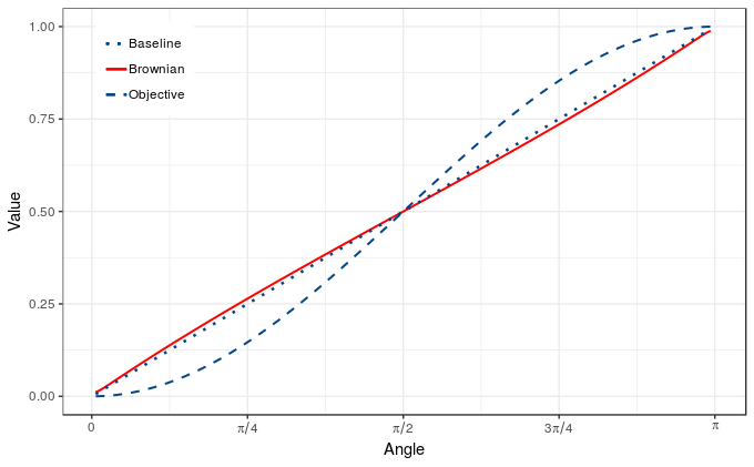
(a) $\alpha=0$.

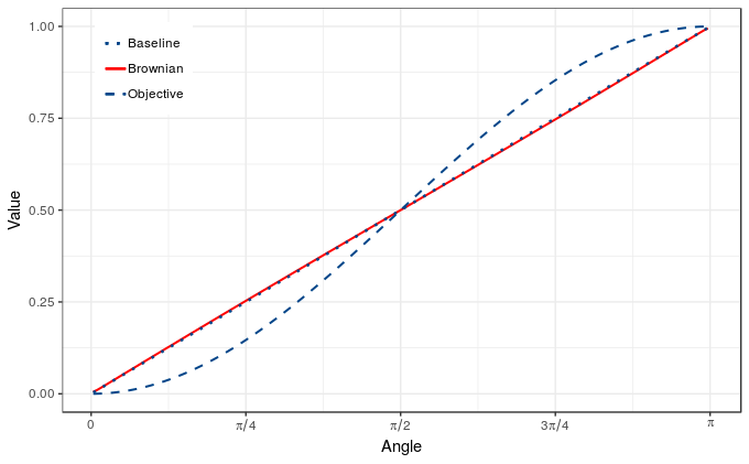
(b) $\alpha=1$.

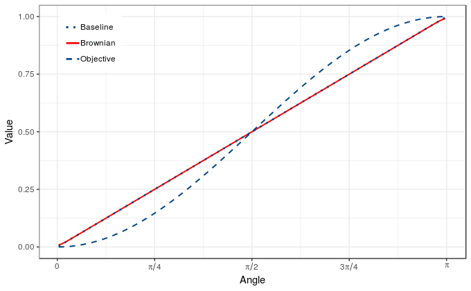
(c) $\alpha=1.61$.

Figure 2: Comparing the performance of three values of the slowdown parameter for the Max-Cut problem.

5.2 Higher-Dimension Brownian Rounding

Our motivating example for considering the higher-dimension Brownian rounding is the Max-DiCut problem: given a directed graph $G=(V,E)$ equipped with non-negative edge weights $a:E\rightarrow\mathbb{R}_{+}$ we wish to find a cut $S\subseteq V$ that maximizes the total weight of edges going out of $S$. The standard semi-definite relaxation for Max-DiCut is the following:

$$\max~{}~{}~{} \sum_{e=(i\rightarrow j)\in E}a_{e}\cdot\frac{\left({\bf w}_{0}+{\bf w}_{i}\right)\cdot\left({\bf w}_{0}-{\bf w}_{j}\right)}{4}$$

$$s.t.~{}~{}~{} {\bf w}_{i}\cdot{\bf w}_{i}=1 \forall i=0,1,...,n$$

$$\|{\bf w}_{i}-{\bf w}_{j}\|^{2}+\|{\bf w}_{j}-{\bf w}_{k}\|^{2}\geq\|{\bf w}_{i}-{\bf w}_{k}\|^{2} \forall i,j,k=0,1,...,n$$

In the above, the unit vector ${\bf w}_{0}$ denotes the cut $S$, whereas $-{\bf w}_{0}$ denotes $\overline{S}$. We also include the triangle inequalities which are valid for any valid relaxation.

The sticky Brownian rounding algorithm for Max-DiCut fails to give a good performance guarantee. Thus we design a high-dimensional variant of the algorithm that incorporates the inherent asymmetry of the problem. Let us now describe the high-dimensional Brownian rounding algorithm. It is similar to the original Brownian rounding algorithm given for Max-Cut, except that it evolves in $\mathbb{R}^{n+1}$ with one additional dimension for ${\bf w}_{0}$. Let ${\bf W}\in\mathbb{R}^{(n+1)\times(n+1)}$ denote the positive semi-definite correlation matrix defined by the vectors ${\bf w}_{0},{\bf w}_{1},\ldots,{\bf w}_{n}$, i.e., for every $0\leq i,j\leq n$ we have that: ${\bf W}_{i,j}={\bf w}_{i}\cdot{\bf w}_{j}$. The algorithm starts at the origin and perform a sticky Brownian motion inside the $[\pm 1]^{n+1}$ hypercube whose correlations are governed by ${\bf W}$.

As before, we achieve this by defining a random process $\left\{{\bf X}_{t}\right\}_{t\geq 0}$ as follows:

$${\bf X}_{t}={\bf W}^{\nicefrac{{1}}{{2}}}{\bf B}_{t},$$

where $\left\{{\bf B}_{t}\right\}_{t\geq 0}$ is the standard Brownian motion in $\mathbb{R}^{n+1}$ starting at the origin and ${\bf W}^{\nicefrac{{1}}{{2}}}$ is the square root matrix of ${\bf W}$. Additionally, we force $\left\{{\bf X}_{t}\right\}_{t\geq 0}$ to stick to the boundary of the $[\pm 1]^{n+1}$ hypercube, i.e., once a coordinate of ${\bf X}_{t}$ equals either $1$ or $-1$ it is fixed and remains unchanged indefinitely. This description can be formalized the same way we did for the Max-Cut problem. Below we use $\sigma$ for the time at which ${\bf X}_{\sigma}\in\{-1,1\}^{n+1}$, which has finite expectation.

Unlike the Brownian rounding algorithm for Max-Cut, we need to take into consideration the value ${\bf w}_{0}$ was rounded to, i.e., $\left({\bf X}_{\sigma}\right)_{0}$, since the zero coordinate indicates $S$. Formally, the output $S\subseteq V$ is defined as follows:

$$S=\left\{i\in V:\left({\bf X}_{\sigma}\right)_{i}=\left({\bf X}_{\sigma}\right)_{0}\right\}.$$

To simplify the rest of the presentation, let us denote $Z_{i}:=\left({\bf X}_{\sigma}\right)_{i}$ for every $i=0,1,\ldots,n$.

The event that an edge $(i\rightarrow j)\in E$ is an outgoing edge from $S$, i.e., $i\in S$ and $j\in\overline{S}$, involves three random variables: $Z_{i}$, $Z_{j}$, and $Z_{0}$. Formally, the above event happens if and only if $Z_{i}=Z_{0}$ and $Z_{j}\neq Z_{0}$. We now show how events on any triplet of the random variables $Z_{0},Z_{1},\ldots,Z_{n}$ can be precisely calculated. To simplify the presentation, denote the following for every $i,j,k=0,1,2,\ldots,n$ and $\alpha,\beta,\gamma\in\left\{\pm 1\right\}$:

$$p_{i}(\alpha) \triangleq\Pr\left[Z_{i}=\alpha\right]$$

$$p_{ij}(\alpha,\beta) \triangleq\Pr\left[Z_{i}=\alpha,Z_{j}=\beta\right]$$

$$p_{ijk}(\alpha,\beta,\gamma) \triangleq\Pr\left[Z_{i}=\alpha,Z_{j}=\beta,Z_{k}=\gamma\right]$$

Observation 3.

The following two hold:

1. $p_{i}(\alpha)=p_{i}(-\alpha)$, $p_{ij}(\alpha,\beta)=p_{ij}(-\alpha,-\beta)$, and $p_{ijk}(\alpha,\beta,\gamma)=p_{ijk}(-\alpha,-\beta,-\gamma)$ for every $i,j,k=0,1,2,\ldots,n$ and $\alpha,\beta,\gamma\in\left\{\pm 1\right\}$.

2. $p_{i}(\alpha)=\nicefrac{{1}}{{2}}$ for every $i=0,1,2,\ldots,n$ and $\alpha\in\left\{\pm 1\right\}$.

The proof of Observation 3 follows immediately from symmetry.

The following lemmas proves that every conjunction event that depends on three variables from $Z_{0},Z_{1},Z_{2},\ldots,Z_{n}$ can be precisely calculated.

Lemma 15.

For every $i,j,k=0,1,2,\ldots,n$ and $\alpha,\beta,\gamma\in\left\{\pm 1\right\}$:

$$p_{ijk(\alpha,\beta,\gamma)}=\frac{1}{2}\left[p_{ij}(\alpha,\beta)+p_{ik}(\alpha,\gamma)+p_{jk}(\beta,\gamma)-\frac{1}{2}\right].$$

Proof.

$$1-p_{ijk}(\alpha,\beta,\gamma) =1-p_{ijk}(-\alpha,-\beta,-\gamma)$$

$$=\Pr\left[Z_{i}=\alpha\vee Z_{j}=\beta\vee Z_{k}=\gamma\right]$$

$$=p_{i}(\alpha)+p_{j}(\beta)+p_{k}(\gamma)-p_{ij}(\alpha,\beta)-p_{ik}(\alpha,\gamma)-p_{jk}(\beta,\gamma)+p_{ijk}(\alpha,\beta,\gamma).$$

The first equality follows from property (1) of Observation 3. The second equality follows from De-Morgan’s law. The third equality follows from the inclusion and exclusion principle. Isolating $p_{ijk}(\alpha,\beta,\gamma)$ above and using property (2) of Observation 3 concludes the proof. ∎

Let us now consider the case study problem Max-DiCut. One can verify that an edge $(i\rightarrow j)\in E$ is a forward edge crossing the cut $S$ if and only if the following event happens: $\left\{Z_{i}=Z_{0}\neq Z_{j}\right\}$ (recall that $Z_{0}$ indicates $S$). Thus, the value of the Brownian rounding algorithm, when considering only the edge $(i\rightarrow j)$, equals $p_{0ij}(1,1,-1)+p_{0ij}(-1,-1,1)$. Lemma 15 above shows that if one knows the values of $p_{ij}(\alpha,\beta)$ for every $i,j=0,1\ldots,n$ and $\alpha,\beta\in\{\pm 1\}$, then $p_{0ij}(1,1,-1)$ and $p_{0ij}(-1,-1,1)$ can be calculated (thus deriving the exact probability that $(i\rightarrow j)$ is a forward edge crossing $S$).

How can we calculate $p_{ij}(\alpha,\beta)$ for every $i,j=0,1\ldots,n$ and $\alpha,\beta\in\{\pm 1\}$? Fix some $i$, $j$, $\alpha$ and $\beta$. We note that Theorem 4 can be used to calculate $p_{ij}(\alpha,\beta)$. The reason is that: $(1)$ Theorem 4 provides the value of $p_{ij}(-1,1)+p_{ij}(1,-1)$; $(2)$ $p_{ij}(-1,-1)+p_{ij}(-1,1)+p_{ij}(1,-1)+p_{ij}(1,1)=1$; and $(3)$ $p_{ij}(-1,-1)=p_{ij}(1,1)$ and $p_{ij}(-1,1)=p_{ij}(1,-1)$ from symmetry. We conclude that using Theorem 4 we can exactly calculate the probability that $(i\rightarrow j)$ is a forward edge crossing $S$, and obtain that this probability equals:

$$\frac{1}{2}(p_{0j}+p_{ij}-p_{0i}),$$

where $p_{ij}$ is the probability that $i$ and $j$ are separated as given by Theorem 4.

Similarly to Max-2SAT, not all triplets of angles $\{\theta_{0i},\theta_{0j},\theta_{ij}\}$ are possible due to the triangle inequality constraints (here $\theta_{ij}$ indicates the angle between ${\bf w}_{i}$ and ${\bf w}_{j}$). Let us denote by $\mathcal{F}$ the collection of all possible triplet of angles for the Max-DiCut problem. Then, we can lower bound the approximation guarantee of the Brownian rounding algorithm as follows:

$$\min_{(\theta_{0i},\theta_{0j},\theta_{ij})\in\mathcal{F}}\left\{\frac{\frac{1}{2}(p_{0j}+p_{ij}-p_{0i})}{\frac{1}{4}(1-\cos(\theta_{0j})+\cos(\theta_{0i})-\cos(\theta_{ij}))}\right\}.$$

This results in the following theorem.

Theorem 11.

The high dimensional Brownian rounding algorithm achieves an approximation ratio of 0.79 for the Max-DiCut problem.

We also remark that we can introduce slowdown (as discussed in Section 5.1 to the high dimensional Brownian rounding algorithm. Numerically, we show that this improves the performance to $0.79$-approximation.

6 Acknowledgements

The authors are grateful to Assaf Naor and Ronen Eldan for sharing their manuscript with us. SA would like to thank Gantumur Tsogtgerel for bringing the Maximum Principle to our attention, and Christina C. Christara for helping us compare various numerical PDE solvers. SA and AN thank Allan Borodin for useful discussions during the initial stages of this research. GG would like to thank Anupam Gupta and Ian Tice for useful discussion, and for also pointing out the Maximum Principle.

SA and AN were supported by an NSERC Discovery Grant (RGPIN-2016-06333). MS was supported by NSF grant CCF-BSF:AF1717947. Some of this work was carried out while AN and NB were visitors at the Simons Institute program on Bridging Discrete and Continuous Optimization, partially supported by NSF grant #CCF-1740425.

Appendix A Definition of Brownian Motion

For completeness, we recall the definition of standard Brownian motion.

Definition 1.

A stochastic process $\{{\bf B}_{t}\}_{t\geq 0}$ taking values in $\mathbb{R}^{n}$ is called an $n$-dimensional Brownian motion started at ${\bf x}\in\mathbb{R}^{n}$ if

• ${\bf B}_{0}={\bf x}$,

• the process has independent increments, i.e. for all $N$ and all times $0\leq t_{1}\leq t_{2}\leq\ldots\leq t_{N}$, the increments ${\bf B}_{t_{N}}-{\bf B}_{t_{N-1}}$, ${\bf B}_{t_{N}-1}-{\bf B}_{t_{N-2}}$, $\ldots$, ${\bf B}_{t_{2}}-{\bf B}_{t_{1}}$ are independent random variables,

• for all $t\geq 0$ and all $h>0$, the increment ${\bf B}_{t+h}-{\bf B}_{t}$ is distributed as a Gaussian random variable with mean $\mathbf{0}$ and covariance matrix equal to the identity $\mathbf{I}_{n}$,

• the function $f(t)={\bf B}_{t}$ is almost surely continuous.

The process $\{{\bf B}_{t}\}_{t\geq 0}$ is called standard Brownian motion if ${\bf x}=0$.

The fact that this definition is not empty, i.e. that such a stochastic process exists, is non-trivial. The first rigorous proof of this fact was given by Wiener [52]. We refer the reader to the book [43] for a thorough introduction to Brownian motion and its properties.

Appendix B Omitted Proofs from Section 2

We start with a brief primer about special functions with an emphasis on the lemmas and identities that will be useful for our analysis. We recommend the excellent introductions in Andrews et al. [4], Beals and Wong [18] for a thorough introduction.

B.1 Special Functions: A Primer

While there is no common definition of special functions, three basic functions, $\Gamma$, $\beta$ and the hypergeometric functions ${}_{p}F_{q}$ show up in nearly all treatments of the subject. We will define them and some useful relationships between them.

Definition 2 (Gamma Function).

The gamma function is defined as

$$\Gamma(z):=\int_{0}^{\infty}x^{z-1}e^{-x}dx.$$

for all complex numbers $z$ with non-negative real part, and analytically extended to all $z\neq 0,-1,-2,...$.

Fact 1.

Recall that the gamma function satisfies the recurrence $\Gamma(z+1)=z\Gamma(z)$ and it follows easily from the definition that $\Gamma(1)=1$. In particular, when $n$ is a positive integer, $\Gamma(n+1)=n!$

Definition 3 (Beta Function).

The beta function $\beta(a,b)$ is defined for complex numbers $a$ and $b$ with $\mathrm{Re}(a)>0,\mathrm{Re}(b)>0$ by

$$\beta(a,b)=\int_{0}^{1}s^{a-1}(1-s)^{b-1}ds.$$

Clearly, $\beta(a,b)=\beta(b,a)$. Setting $s=u/(u+1)$ gives the following alternate form.

$$\beta(a,b)=\int_{0}^{\infty}u^{a-1}\left(\frac{1}{1+u}\right)^{a+b}du$$

Lemma 16.

(Theorem 1.1.4 in [4]) The beta function can be expressed in terms of the gamma function using the following identity:

$$\beta(a,b)=\frac{\Gamma(a)\Gamma(b)}{\Gamma(a+b)}$$

We will use the following very useful fact.

Lemma 17.

( Exercise 2.2 in [18])

$$\int_{0}^{\pi/2}\sin^{a-1}\theta\cos^{b-1}\theta d\theta=\frac{1}{2}\beta(a/2,b/2)$$

The next family of functions we utilize are the hypergeometric functions.

Definition 4 (Hypergeometric Function).

The hypergeometric function ${}_{p}F_{q}{\left[\genfrac{.}{.}{0.0pt}{}{a_{1}{\mathchar 44\relax}\mskip 8.0mu\dots{\mathchar 44\relax}\mskip 8.0mua_{p}}{b_{1}{\mathchar 44\relax}\mskip 8.0mu\dots{\mathchar 44\relax}\mskip 8.0mub_{q}};z\right]}$ is defined as

$${}_{p}F_{q}{\left[\genfrac{.}{.}{0.0pt}{}{a_{1}{\mathchar 44\relax}\mskip 8.0mu\dots{\mathchar 44\relax}\mskip 8.0mua_{p}}{b_{1}{\mathchar 44\relax}\mskip 8.0mu\dots{\mathchar 44\relax}\mskip 8.0mub_{q}};z\right]}:=\sum_{n=0}^{\infty}\frac{(a_{1})_{n}\cdots(a_{p})_{n}}{(b_{1})_{n}\cdot(b_{q})_{n}}\frac{z^{n}}{n!}$$

where the Pochhammer symbol (rising factorial) is defined inductively as

$$(a)_{n}:=a(a+1)\cdots(a+n-1)\text{ and }(a)_{0}=1.$$

A very simple but useful way to write the binomial theorem using the Pochhammer symbol is

$$(1-x)^{-a}=\sum_{n=0}^{\infty}\frac{(a)_{n}}{n!}x^{n}.$$

The Pochhammer symbol also satisfies the formula $(a)_{n}=\Gamma(a+n)/\Gamma(a)$.

A useful connection between the hypergoemetric function ${}_{2}F_{1}$ and the gamma function is given in the following lemma.

Lemma 18 (Euler’s Integral Representation).

[Theorem 2.2.1 in [4]] If $\mathrm{Re}(c)>\mathrm{Re}(b)>0$ then

$${}_{2}F_{1}{\left[\genfrac{.}{.}{0.0pt}{}{a{\mathchar 44\relax}\mskip 8.0mub}{c};x\right]}=\frac{\Gamma(c)}{\Gamma(b)\Gamma(c-b)}\int_{0}^{1}t^{b-1}(1-s)^{c-b-1}(1-xs)^{-a}ds$$

where we assume that $(1-xs)^{-a}$ takes its principal value.

Definition 5.

The incomplete beta integral is defined as

$$\beta_{x}(a,b)=\int_{0}^{x}t^{a-1}(1-t)^{b-1}dt,$$

and is well-defined for $\mathrm{Re}(a)>0$ and $x\notin[1,\infty)$.

Lemma 17 easily extends to the incomplete beta integral too, as captured in the following lemma.

Lemma 19.

$$\int_{0}^{\phi}\sin^{a-1}\theta\cos^{b-1}\theta d\theta=\frac{1}{2}\beta_{\sin^{2}\phi}(a/2,b/2)$$

Proof.

Let $\sin\theta=t$, then $\cos\theta=\sqrt{1-t^{2}}$ and $(\cos\theta)d\theta=dt$, and we get

$$\int_{0}^{\phi}\sin^{a-1}\theta\cos^{b-1}\theta d\theta=\int_{0}^{\sin(\phi)}t^{a-1}(1-t^{2})^{(b-2)/2}dt.$$

Setting $s=t^{2}$ gives

$$\int_{0}^{\sin^{2}(\phi)}(1/2)s^{(a-2)/2}(1-s)^{(b-2)/2}ds=(1/2)\beta_{\sin^{2}\phi}(a/2,b/2).$$

This completes the proof. ∎

The following identity relates the incomplete beta integral to hypergeometric functions.

Lemma 20 (Gauss’s Identity).

[Exercise 8.7 in [18]]

$$\beta_{x}(a,b)=\int_{0}^{x}t^{a-1}(1-t)^{b-1}dt=\frac{x^{a}}{a}\cdot{}_{2}F_{1}{\left[\genfrac{.}{.}{0.0pt}{}{a{\mathchar 44\relax}\mskip 8.0mu1-b}{a+1};x\right]}$$

Proof.

It is natural to substitute $t=sx$, as we can now integrate from $s=0$ to $1$. This gives

$$\int_{0}^{1}x^{a-1}s^{a-1}(1-sx)^{b-1}xds=x^{a}\int_{0}^{1}s^{a-1}(1-sx)^{b-1}ds$$

Using the integral form given in Lemma 18 with $1-b$ in the place of $a$, $a$ in the place of $b$, and $a+1$ in the place of $c$, we get that the integral equals

$$x^{a}\frac{\Gamma(a)\Gamma(1)}{\Gamma(a+1)}\cdot{}_{2}F_{1}{\left[\genfrac{.}{.}{0.0pt}{}{1-b{\mathchar 44\relax}\mskip 8.0mua}{a+1};x\right]}=\frac{x^{a}}{a}\cdot{}_{2}F_{1}{\left[\genfrac{.}{.}{0.0pt}{}{1-b{\mathchar 44\relax}\mskip 8.0mua}{a+1};x\right]}$$

By the symmetry in the definition of ${}_{2}F_{1}$ with respect to the first two arguments, the result follows. ∎

B.2 Proof of Theorem 4

First, we will prove the claim, which expresses the function $r(\phi)$ in terms of the incomplete beta function. See 1

Proof.

Recall $r(\phi)=\lvert F_{\theta}(e^{i\phi})-F_{\theta}(1)\rvert$. Furthermore, from Lemma 3, we know that the conformal map maps the arc from $1$ to $i$ to an edge on the rhombus $\mathbb{S}$. Hence we can write $r(\phi)$ as an integral

$$r(\phi) =\int_{0}^{\phi}|F_{\theta}^{\prime}(e^{i\phi})|d\phi=\int_{0}^{\phi}|f_{\theta}(e^{i\phi})|d\phi.$$

Expanding $$f_{\theta} a=\frac{\theta}{\pi} b=1-a$$, and substituting and , we have

$$=\int_{0}^{\phi}|(1-e^{2i\phi})^{a-1}\cdot(1+e^{2i\phi})^{b-1}|d\phi.$$

Expanding this in terms of trigonometric functions, and simplifying using double angle formulas, we get

$$=\int_{0}^{\phi}|(2\cdot e^{i\phi}\cdot\sin\phi)^{a-1}\cdot(2\cdot e^{-i\phi}\cdot\cos\phi)^{b-1}|d\phi$$

$$=\int_{0}^{\phi}|2^{a+b-2}|\cdot|e^{i\phi(a-1)}|\cdot|\sin\phi^{a-1}|\cdot|e^{-i\phi(b-1)}|\cdot|\cos\phi^{b-1}|d\phi.$$

Since $$|e^{i\phi(a-1)}|=|e^{i\phi(b-1)}|=1$$ and the remaining terms are positive, we drop the norms.

$$=\int_{0}^{\phi}\frac{1}{2}(\sin\phi)^{a-1}(\cos\phi)^{b-1}d\phi$$

$$=\frac{1}{4}\beta_{\sin^{2}\phi}(a/2,b/2)$$ by Lemma 19.

∎

By substituting $\phi=\pi/2$ we immediately get the following corollary:

Corollary 3.

The length of the side of rhombus is given by $r=r(\pi/2)=\nicefrac{{1}}{{4}}\cdot\beta(a/2,b/2)$.

The claim below will characterize the integral of the incomplete beta function which will be important for us later.

See 2

Proof.

By Lemma 19, the left hand side equals

$$\int_{0}^{\pi/2}\beta_{\sin^{2}\phi}\left(\frac{a}{2},\frac{b}{2}\right)d\phi$$

$$=\int_{0}^{\pi/2}\frac{2\left(\sin^{2}\phi\right)^{a/2}}{a}{}_{2}F_{1}{\left[\genfrac{.}{.}{0.0pt}{}{\frac{a}{2}{\mathchar 44\relax}\mskip 8.0mu1-\frac{b}{2}}{\frac{a}{2}+1};\sin^{2}\phi\right]}d\phi$$ By Lemma 20

$$=\int_{0}^{\pi/2}\frac{2(\sin\phi)^{a}}{a}{}_{2}F_{1}{\left[\genfrac{.}{.}{0.0pt}{}{\frac{a}{2}{\mathchar 44\relax}\mskip 8.0mu\frac{a+1}{2}}{\frac{a}{2}+1};\sin^{2}\phi\right]}d\phi b=1-a$$ Substituting

$$=\frac{2}{a}\int_{0}^{\pi/2}\Big{(}\sum_{n=0}^{\infty}\frac{(a/2)_{n}(a/2+1/2)_{n}}{(a/2+1)_{n}}\frac{(\sin\phi)^{2n+a}}{n!}\Big{)}d\phi$$ Expand using Definition 4

$$=\frac{2}{a}\sum_{n=0}^{\infty}\Big{(}\int_{0}^{\pi/2}(\sin\phi)^{2n+a}d\phi\Big{)}\frac{(a/2)_{n}(a/2+1/2)_{n}}{(a/2+1)_{n}\cdot n!}$$ (*)

We take a brief interlude to analyze the integral in the parenthesis above:

$$\int_{0}^{\pi/2}\left(\sin\phi\right)^{2n+a}d\phi =\frac{1}{2}\beta(n+a/2+1/2,1/2)$$ By Lemma 17

$$=\frac{\Gamma(1/2)}{2}\frac{\Gamma(n+a/2+1/2)}{\Gamma(n+a/2+1)}$$ By Lemma 16

$$=\frac{\Gamma(1/2)}{2}\frac{(a+1/2)_{n}\Gamma(a/2+1/2)}{(a/2+1)_{n}\Gamma(a+1)}$$

$$=\frac{\beta(a/2+1/2,1/2)}{2}\frac{(a/2+1/2)_{n}}{(a/2+1)_{n}}.$$

Going back and substituting the above result into the Equation *, we get

$$=\frac{\beta(a/2+1/2,1/2)}{a}\left(\sum_{n=0}^{\infty}\frac{(a/2)_{n}(a/2+1/2)_{n}(a/2+1/2)_{n}}{n!(a/2+1)_{n}(a+1)_{n}}\right)$$

$$=\frac{\beta(a/2+1/2,1/2)}{a}\cdot{}_{3}F_{2}{\left[\genfrac{.}{.}{0.0pt}{}{\frac{1+a}{2}{\mathchar 44\relax}\mskip 8.0mu\frac{1+a}{2}{\mathchar 44\relax}\mskip 8.0mu\frac{a}{2}}{\frac{a}{2}+1{\mathchar 44\relax}\mskip 8.0mu\frac{a}{2}+1};1\right]}$$

∎

Armed with Claim 2 and Corollary 3, we can prove Theorem 4. See 4

Proof.

Substituting $r=r(\pi/2)$ below, by Lemma 4 we have that the probability of separating the vertices is

$$\frac{2}{\pi}\int_{\phi=0}^{\pi/2}1-\frac{r(\phi)}{r}d\phi,$$

or equivalently, the probability of not separating them is

$$\frac{2}{\pi}\int_{\phi=0}^{\pi/2}\frac{r(\phi)}{r}d\phi$$

Expanding the above using Claim 1, we get that this equals

$$\frac{2}{\pi}\frac{4}{\beta(a/2,b/2)}\int_{\phi=0}^{\pi/2}\frac{1}{4}\beta_{\sin^{2}\psi}(a/2,(1-a)/2)d\psi.$$

Expanding the right hand side integral using Claim 2, we get

$$=\frac{2}{\pi}\frac{1}{\beta(a/2,b/2)}\cdot\frac{\beta(a/2+1/2,1/2)}{a}\cdot{}_{3}F_{2}(1/2+a/2,1/2+a/2,a/2;a/2+1,a+1;1).$$

Using Lemma 16 and the fact that $$\Gamma(1/2)^{2}=\pi$$ we can simplify this to

$$=\frac{\Gamma(a+1/2)}{\Gamma(1/2-a/2)\Gamma(a/2+1)^{2}}\cdot{}_{3}F_{2}(1/2+a,1/2+a/2,a/2;a/2+1,a+1;1).$$

∎

B.3 Proof of Theorem 7

First, we rewrite $r$ in a form that will be useful later.

Claim 3.

$$2\int_{0}^{\pi/2}r(\phi)d\phi=\int_{0}^{\pi/2}\phi(\sin\phi)^{b-1}(\cos\phi)^{a-1}d\phi$$

Proof.

The left hand side equation can be written as

$$2\int_{0}^{\pi/2}r(\phi)d\phi=\int_{0}^{\pi/2}\frac{1}{2}\beta_{\sin^{2}{\phi}}(a/2,b/2)d\phi=\int_{0}^{\pi/2}\left(\int_{0}^{\phi}(\sin\psi)^{a-1}(\cos\psi)^{b-1}d\psi\right)d\phi$$

Applying integration by parts: $\int pdq=[pq]-\int qdp$ with $q=\pi/2-\phi$ and $p=\int_{0}^{\phi}(\sin\psi^{a-1})(\cos\psi)^{b-1}d\psi$ gives

$$\Big{[}(\pi/2-\phi)\int_{0}^{\phi}(\sin\psi^{a-1})(\cos\psi)^{b-1}d\psi\Big{]}_{0}^{\pi/2}+\int_{0}^{\pi/2}(\pi/2-\phi)\frac{d}{d\phi}\int_{0}^{\phi}(\sin\psi^{a-1})(\cos\psi)^{b-1}d\psi$$

The first term is $0$, and using Fundamental Theorem of Calculus, the second term is

$$\int_{0}^{\pi/2}(\pi/2-\phi)(\sin\phi)^{a-1}(\cos\phi)^{b-1}d\phi$$

Substituting $\phi$ for $\pi/2-\phi$ gives

$$\int_{0}^{\pi/2}\phi(\sin\phi)^{b-1}(\cos\phi)^{a-1}d\phi.$$

∎

Next, we claim that

Claim 4.

When $\theta=(1-\epsilon)\pi$, we can say

$$2\int_{0}^{\pi/2}r(\phi)d\phi\leq 2\cdot\Big{(}1+O(\epsilon\log(1/\epsilon))\Big{)}.$$

Proof.

Using Claim 3, we can write

$$2\int_{0}^{\pi/2}r(\phi)d\phi =\int_{0}^{\pi/2}\phi(\sin\phi)^{b-1}(\cos\phi)^{a-1}d\phi$$

$$=\int_{0}^{\pi/2}\frac{\phi}{\sin\phi}(\tan\phi)^{\epsilon}d\phi$$

Since $\frac{x}{\sin(x)}\leq 2$ for $0\leq x\leq\nicefrac{{\pi}}{{2}}$, to prove the claim it suffices to show that

$$\int_{0}^{\pi/2}\left((\tan\phi)^{\epsilon}-1\right)d\phi=O(\epsilon\log(1/\epsilon)).$$

Let $\phi_{0}=\arctan(1/\epsilon)$. We will break the above integral into two parts and deal with each separately:

$$\int_{0}^{\pi/2}\left((\tan\phi)^{\epsilon}-1\right)d\phi=\int_{0}^{\phi_{0}}\left((\tan\phi)^{\epsilon}-1\right)+\int_{\phi_{0}}^{\pi/2}\left((\tan\phi)^{\epsilon}-1\right).$$

Case 1 for $\phi\leq\phi_{0}$,

$$(\tan\phi)^{\epsilon}\leq\left(\frac{1}{\epsilon}\right)^{\epsilon}=\exp(\epsilon\ln(1/\epsilon))=1+O(\epsilon\log(1/\epsilon)),$$

so

$$\int_{0}^{\phi_{0}}\left((\tan\phi)^{\epsilon}-1\right)d\phi=O(\epsilon\log(1/\epsilon)).$$

Case 2 For $\phi>\phi_{0}$,

$$\int_{\phi_{0}}^{\pi/2}\left((\tan\phi)^{\epsilon}-1\right)d\phi \leq\int_{\phi_{0}}^{\pi/2}1/(\cos\phi)^{\epsilon}d\phi$$

$$=\int_{0}^{\pi/2-\phi_{0}}(1/\sin\phi)^{\epsilon}d\phi \text{ Since}\sin(x)=\cos(\pi/2-x)$$

$$\leq\int_{0}^{\pi/2-\phi_{0}}(2/\phi)^{\epsilon}d\phi \text{Since }1\leq\nicefrac{{x}}{{\sin(x)}}\leq 2$$

$$\leq 2^{\epsilon}\frac{(\pi/2-\phi_{0})^{1-\epsilon}}{1-\epsilon}$$

$$\leq(\pi/2-\phi_{0})(1+O(\epsilon)).$$

Finally, we note that $\pi/2-\phi_{0}\leq\tan(\pi/2-\phi_{0})=1/\tan(\phi_{0})=\epsilon$. ∎

See 7

Proof.

Let $a=1-\epsilon$ and $b=\epsilon$.

As discussed in Lemma 4, the non-separation probability is

$$\frac{2}{\pi r}\int_{0}^{\pi/2}r(\phi)d\phi$$

where $r=r(\pi/2)$. So we will compute the asymptotics of $r:=r(\pi/2)$ and $\int_{0}^{\pi/2}2\cdot r(\phi)d\phi$ as $\varepsilon\to 0$.

First we compute the asymptotics of $r$ as $\varepsilon\to 0$. Recall that

$$r =(1/4)\beta(a/2,b/2)$$ By Corollary 3

$$=\frac{\Gamma((1-\epsilon)/2)\Gamma(\epsilon/2)}{4\Gamma(1/2)}$$ By Lemma 16

$$=\frac{\Gamma((1-\epsilon)/2)\Gamma(1+\epsilon/2)}{2\epsilon\Gamma(1/2)} \text{ Using }\Gamma(\frac{\epsilon}{2})=\frac{2}{\epsilon}\Gamma(1+\frac{\epsilon}{2})$$

Using the standard fact that $$\Gamma(z+\epsilon)=\Gamma(z)(1+O(\epsilon)) z>0$$ for fixed

$$=\frac{1}{2\epsilon\Gamma(1/2)}(\Gamma(1/2)+O(\epsilon))(\Gamma(1)+O(\epsilon))$$

$$=\frac{1}{(2\epsilon)}+O(1)$$

which implies that

$$1/r=2\epsilon+O(\epsilon)^{2}$$

Using Claim 4, we know that $\int_{0}^{\pi/2}2\cdot r(\phi)d\phi$ is at most $2\cdot\Big{(}1+O(\epsilon\log(1/\epsilon)\Big{)}$. Combining the two, we get the probability of non-separation is $\epsilon\frac{4}{\pi}+O(\epsilon^{2})\approx 1.27\epsilon+O(\epsilon^{2})$. ∎

B.4 Other Missing Proofs

See 1

Proof.

Part 1 is immediate from the continuity and linearity of the map $\mathbf{O}\cdot{\bf W}^{-\nicefrac{{1}}{{2}}}$.

To prove part 2, observe that the $W^{\nicefrac{{1}}{{2}}}$ is given explicitly by the matrix

$${\bf W}^{\frac{1}{2}}=\frac{1}{\sqrt{2}}\cdot\begin{bmatrix}\cos(\frac{\theta}{2})+\sin(\frac{\theta}{2})&\cos(\frac{\theta}{2})-\sin(\frac{\theta}{2})\\ \cos(\frac{\theta}{2})-\sin(\frac{\theta}{2})&\cos(\frac{\theta}{2})+\sin(\frac{\theta}{2})\end{bmatrix}.$$

Taking, its inverse, we get the matrix

$${\bf W}^{-\frac{1}{2}}=\frac{1}{\sqrt{8}}\cdot\begin{bmatrix}\sec(\frac{\theta}{2})+\csc(\frac{\theta}{2})&\sec(\frac{\theta}{2})-\csc(\frac{\theta}{2})\\ \sec(\frac{\theta}{2})-\csc(\frac{\theta}{2})&\sec(\frac{\theta}{2})+\csc(\frac{\theta}{2})\end{bmatrix}.$$

Since ${\bf W}^{-\frac{1}{2}}[-1,1]^{2}$ is the image of a parallelogram, it must also be a parallelogram. Moreover, one can directly check that the diagonals are orthogonal to each other, so it must be a rhombus. It is easy to calculate the angle between the sides and see that it is exactly $\theta$ at the image of $(1,-1)$ and $\pi-\theta$ at the image of $(1,1)$.

Then part 3 follows from the previous parts: if ${\bf X}_{t}$ is one a side or a vertex of $[-1,1]$, then ${\bf Y}_{t}$ is on the corresponding side or vertex of $\mathbb{S}$. ∎

Appendix C Omitted Proofs from Section 3

Recall that, for $0\leq x\leq 1,0\leq y\leq 1$, the function $u(x,y)$ denotes the probability the probability of a clause being satisfied when the random walk walk begins with marginals $(x,y)$ and angle $\theta$. Equivalently, $u(x,y)$ is the probability that the walk, started at $(x,y)$, ends at one of the corners $(0,0)$, $(0,1)$ or $(1,0)$.

See 5

Proof.

Recall that $\tau$ is the first time when ${\bf X}_{t}$ hits the boundary of $[0,1]^{2}$, and $\sigma$ is the first time when ${\bf X}_{t}$ hits a vertex of $[0,1]^{2}$. The function $\phi$ evaluates to $1$ at the vertices $(0,0)$, $(0,1)$, and $(1,0)$, and to $0$ at $(1,1)$. Therefore, by definition, $u({\bf x})=\mathbb{E}^{\bf x}[\phi({\bf X}_{\sigma})]$.

Let us first consider the case when ${\bf x}$ is on the boundary of $[0,1]^{2}$. Then one of the coordinates of ${\bf X}_{t}$ remains fixed for the entire process. Since $\phi$ is affine in each of its arguments, and ${\bf X}_{t}$ is a martingale,

$$\forall{\bf x}\in{\partial}[0,1]^{2}:\ u({\bf x})=\mathbb{E}^{\bf x}[\phi({\bf X}_{\sigma})]=\phi(\mathbb{E}^{\bf x}[{\bf X}_{\sigma}])=\phi({\bf x}).$$

When ${\bf x}$ is in the interior of $[0,1]^{2}$, we have, by the law of total expectation,

$$\forall{\bf x}\in{\operatorname{Int}}[0,1]^{2}:\ u({\bf x})=\mathbb{E}^{\bf x}[\phi({\bf X}_{\sigma})]=\mathbb{E}^{\bf x}[\mathbb{E}^{{\bf X}_{\tau}}[\phi({\bf X}_{\sigma})]]=\mathbb{E}^{\bf x}[\phi({\bf X}_{\tau})].$$

The final equality follows by the special case when the starting point of the random walk is on the boundary of $[0,1]^{2}$. This proves the lemma. ∎

Before we give an outline of the proofs of Lemma 6 and Lemma 8, we prove Lemma 7. This will allow us to give a completely analytic proof of $\frac{3}{4}$.

See 7

Proof.

Clearly, the first set of the constraints are obvious. We focus on the second and the third constraint. Recall that ${\bf v}_{i}=x{\bf v}_{0}+\sqrt{x-x^{2}}{\bf w}_{i}$ and ${\bf v}_{j}=y{\bf v}_{0}+\sqrt{y-y^{2}}{\bf w}_{j}$ where ${\bf w}_{i}$ and ${\bf w}_{j}$ are unit vectors orthogonal to ${\bf v}_{0}$ with $\cos(\theta)={\bf w}_{j}\cdot{\bf w}_{j}$. Thus we have

$${\bf v}_{i}\cdot{\bf v}_{j}=xy+\cos(\theta)\sqrt{x-x^{2}}\sqrt{y-y^{2}}$$

But then we have the following valid constraint from the SDP:

$${\bf v}_{i}\cdot{\bf v}_{j}\geq 0$$

which implies that

$$\cos(\theta)\geq-\sqrt{\frac{xy}{(1-x)(1-y)}}$$

proving the second inequality.

For the other inequality, observe that we have ${\bf v}_{-i}=(1-x){\bf v}_{0}-\sqrt{x-x^{2}}{\bf w}_{i}$ and ${\bf v}_{-j}=(1-y){\bf v}_{0}-\sqrt{y-y^{2}}{\bf w}_{j}$. Then we have

$${\bf v}_{-i}\cdot{\bf v}_{-j}=(1-x)(1-y)+\cos(\theta)\sqrt{x-x^{2}}\sqrt{y-y^{2}}$$

But then we have the following valid constraint from the SDP:

$${\bf v}_{-i}\cdot{\bf v}_{-j}\geq 0$$

which implies that

$$\cos(\theta)\geq-\sqrt{\frac{(1-x)(1-y)}{xy}}$$

proving the third inequality. ∎

To ease the remainder of the presentation we first prove that the Brownian rounding algorithm achieves an approximation of $\nicefrac{{3}}{{4}}$ for Max-2SAT via the maximum principle. In order to achieve that we use the following two functions for different ranges of $\theta$.

• $g_{1}(x,y)=1-xy-\cos(\theta)\sqrt{x-x^{2}}\sqrt{y-y^{2}}$.

• $f(x,y)=1-xy$.

First consider the case when $0\leq\theta\leq\frac{\pi}{2}$. In this case, we show $g_{1}$ satisfies the requirement of the Corollary 2 as well as give an approximation factor of $1$. The last fact is trivially true since $g_{1}$ is exactly the SDP objective.

For conditions of the Corollary 2, we need to show that

$$\frac{\partial^{2}g_{1}}{\partial x^{2}}+\frac{\partial^{2}g_{1}}{\partial y^{2}}+2\cos(\theta)\frac{\partial^{2}g_{1}}{\partial x\partial y} \geq 0 \forall(x,y)\in{\operatorname{Int}}[0,1]^{2}$$

$$g_{1}(x,y) \leq(1-xy) \forall(x,y)\in\partial[0,1]^{2}$$

Since $(x-x^{2})(y-y^{2})=0$ on ${\partial}[0,1]^{2}$, we obtain that $g_{1}(x,y)=1-xy$ on ${\partial}[0,1]^{2}$ as required. It remains to show that

$$\frac{\partial^{2}}{\partial x^{2}}g_{1}(x,y)+\frac{\partial^{2}}{\partial y^{2}}g_{1}(x,y)+2\cos{\theta}\frac{\partial^{2}}{\partial x\partial y}g_{1}(x,y)\geq 0$$

for all $(x,y)\in(0,1)^{2}$. Consider

$$h(x,y):=\frac{\partial^{2}}{\partial x^{2}}g_{1}(x,y)+\frac{\partial^{2}}{\partial y^{2}}g_{1}(x,y)+2\cos{\theta}\frac{\partial^{2}}{\partial x\partial y}g_{1}(x,y).$$

To show $h$ is non-negative, we do the following change of variables in $x=\frac{(1+\sin(a))}{2}$ and $y=\frac{(1+\sin(b))}{2}$ for some $|a|,|b|\leq\frac{\pi}{2}$. Such $a$ and $b$ exist since $0\leq x,y\leq 1$. Now simplifying, we obtain:

$$h\left(\frac{1+\sin(a)}{2},\frac{1+\sin(b)}{2}\right)$$

$$= 2\cos(\theta)\sec^{3}(a)\sec^{3}(b)\Big{[}\left(cos^{2}(a)-\cos^{2}(b)\right)^{2}$$

$$+2\cos^{2}(a)\cos^{2}(b)\left(1-\cos(\theta)\sin(a)\sin(b)-\cos(a)\cos(b)\right)\Big{]}$$

Since $|a|,|b|\leq\frac{\pi}{2}$ and $0\leq\theta\leq\frac{\pi}{2}$, we have that $\sec(a),\sec(b),\cos(\theta)\geq 0$. Thus, it enough to show that

$$1-\cos(\theta)\sin(a)\sin(b)-\cos(a)\cos(b)\geq 0.$$

Since the above expression is linear in $\cos(\theta)$, it is enough to check for extreme values of $\cos(\theta)$ which takes value between $0$ and $1$. It is clearly true when $\cos(\theta)=0$. For $\cos(\theta)=1$, it equals $1-\cos(a-b)$ and is thus non-negative.

Now consider $-1\leq\cos(\theta)\leq 0$. We show that $f(x,y)=1-xy$ satisfies the condition of Corollary 2 and is at least $\frac{3}{4}$ the value of the SDP objective for all feasible $(x,y,\theta)$. First let us focus on the condition of Corollary 2. Clearly, the boundary conditions are satisfied by construction. Note that $\frac{\partial^{2}f(x,y)}{\partial x^{2}}=0$, $\frac{\partial^{2}f(x,y)}{\partial y^{2}}=0$, and that $\frac{\partial^{2}f(x,y)}{\partial x\partial y}=1$. Thus

$$\mathcal{L}f=-\cos(\theta)\geq 0$$

since $\cos(\theta)\leq 0$ as desired.

It remains to show that $f$ provides an approximation guarantee of $\nicefrac{{3}}{{4}}$ in case $\cos(\theta)<0$. Recall that $SDP(x,y,\theta)=1-xy-\cos(\theta)\sqrt{x-x^{2}}\sqrt{y-y^{2}}$ is the contribution of a clause to the SDP’s objective whose two variables $z_{i}$ and $z_{j}$ have marginal values of $x$ and $y$ respectively and that $\cos(\theta)={\bf w}_{i}\cdot{\bf w}_{j}$. We prove the following claim which would imply that we obtain a $\frac{3}{4}$-approximation.

Claim 5.

For any $x,y,\theta$ that satisfy the feasibility conditions in Lemma 7 and $\cos(\theta)<0$, we have

$$g(x,y)\geq\frac{3}{4}SDP(x,y,\theta).$$

Proof.

From Lemma 7, we have

$$-\cos(\theta)\leq\min\left\{\sqrt{\frac{xy}{(1-x)(1-y)}},\sqrt{\frac{(1-x)(1-y)}{xy}}\right\}.$$

Observe that we have $g(x,y)\geq\frac{3}{4}SDP(x,y,\theta)$, if

$$(1-xy)\geq-3\cos(\theta)\sqrt{(x-x^{2})(y-y^{2})}.$$

First, suppose $xy\leq\frac{1}{4}$. Then

$$-3\cos(\theta)\sqrt{(x-x^{2})(y-y^{2})} \leq 3\sqrt{\frac{xy}{(1-x)(1-y)}}\cdot\sqrt{(x-x^{2})(y-y^{2})}=3xy$$

$$\leq 1-xy$$

Else, if $xy\geq\frac{1}{4}$, then we have

$$1-xy+3\cos(\theta)\sqrt{(x-x^{2})(y-y^{2})} \geq 1-xy-3\sqrt{\frac{(1-x)(1-y)}{xy}}\cdot\sqrt{(x-x^{2})(y-y^{2})}$$

$$= -2+3x+3y-4xy$$

Over all $1\geq x\geq 0,1\geq y\geq 0$ with fixed $xy$, the quantity $2+3x+3y-4xy$ is minimized when $x=y$. Since $xy\geq\frac{1}{4}$, we must have $x\geq\frac{1}{2}$. But then it becomes $-2(1-3x+2x^{2})=-2(1-2x)(1-x)\geq 0$ since $\frac{1}{2}\leq x\leq 1$. This proves the $\frac{3}{4}$-approximation. ∎

We now give a brief outline of the proof of Lemma 6 and Lemma 8. The complete proofs involve long sum of square expression that are available at [1]. See 6

Proof.

Feasibility of $g_{1}(x,y)$. We already showed in the above proof of $\frac{3}{4}$-approximation.

Feasibility of $g_{2}(x,y)$. Now we consider $g_{2}(x,y)=1-xy-2\cos(\theta)(x-x^{2})(y-y^{2})$. Since $(x-x^{2})(y-y^{2})=0$ on ${\partial}[0,1]^{2}$, we obtain that $g_{2}(x,y)=1-xy$ on ${\partial}[0,1]^{2}$ as required. It remains to show that

$$\mathcal{L}g_{2}=\frac{\partial^{2}}{\partial x^{2}}g_{2}(x,y)+\frac{\partial^{2}}{\partial y^{2}}g_{2}(x,y)+2\cos{\theta}\frac{\partial^{2}}{\partial x\partial y}g_{2}(x,y)\geq 0$$

for all $(x,y)\in(0,1)^{2}$ for any $0\geq\cos(\theta)\geq-\frac{1}{2}$. A simple calculation allows us to obtain that

$$\mathcal{L}g_{2}=-2\cos(\theta)\left(1+2x^{2}+2y^{2}+2\cos(\theta)-2x-2y-4y\cos(\theta)-4x\cos(\theta)+8xy\cos(\theta)\right).$$

Since $-2\cos(\theta)>0$, it is enough to show that for any $0\leq x\leq 1$ and $0\leq y\leq 1$,

$$h(x,y)=1+2x^{2}+2y^{2}+2\cos(\theta)-2x-2y-4y\cos(\theta)-4x\cos(\theta)+8xy\cos(\theta)\geq 0.$$

We now prove the above inequality. Since the above expression is linear in $\cos(\theta)$, for any fixed $x,y$ the minimum appears at either $\cos(\theta)=0$ or $\cos(\theta)=-\frac{1}{2}$. First consider $\cos(\theta)=0$. In this case, we obtain

$$h(x,y)=1+2x^{2}+2y^{2}-2x-2y=\frac{1}{2}\left(1-2x\right)^{2}+\frac{1}{2}\left(1-2y\right)^{2}\geq 0$$

as required.

Now if $\cos(\theta)=-\frac{1}{2}$, we obtain

$$h(x,y)=2x^{2}+2y^{2}-4xy=2(x-y)^{2}\geq 0$$

as required. This proves $\mathcal{L}g_{2}\geq 0$.

Feasibility of $g_{3}(x,y)$. Now we consider $g_{3}(x,y)=1-xy-\frac{1}{2}(1+5\cos(\theta))(x-x^{2})(y-y^{2})(x+y)(2-x-y)$ on ${\partial}[0,1]^{2}$, we obtain that $g_{2}(x,y)=1-xy$ on ${\partial}[0,1]^{2}$ as required. It remains to show that

$$\mathcal{L}g_{3}=\frac{\partial^{2}}{\partial x^{2}}g_{3}(x,y)+\frac{\partial^{2}}{\partial y^{2}}g_{3}(x,y)+2\cos{\theta}\frac{\partial^{2}}{\partial x\partial y}g_{3}(x,y)\geq 0$$

for all $(x,y)\in(0,1)^{2}$ for any $-\frac{1}{2}\geq\cos(\theta)\geq-1$.

To show $\mathcal{L}g_{3}\geq 0$, we consider $\mathcal{L}g_{3}=p(x,y,\cos(\theta))$ as a polynomial in $x,y$ and $\cos(\theta)$. Replacing $z=\cos(\theta)$, our aim is to show $p(x,y,z)\geq 0$ if $0\leq x,y\leq 1$ and $-\frac{1}{2}\leq z\leq-1$. Equivalently, we need to show $p(x,y,z)\geq 0$ whenever $r_{1}(x,y,z):=x-x^{2}\geq 0$, $r_{2}(x,y,z):=y-y^{2}\geq 0$ and $r_{3}(x,y,z):=-(z+\frac{1}{2})\geq 0$ and $r_{4}(x,y,z):=(z+1)\geq 0$. This we show by obtaining polynomials $q_{i}(x,y,z)$ for $i=0,1,2,3,4$ such that $q_{i}$ is a sum of square polynomial of fixed degree and we have

$$p(x,y,z)=q_{0}(x,y,z)+\sum_{i=1}^{4}q_{i}(x,y,z)r_{i}(x,y,z).$$

Observe that above polynomial inequality shows the desired inequality. Indeed evaluate the above identity for any $0\leq x,y\leq 1$ and $-\frac{1}{2}\geq z\geq-1$. Clearly, the RHS is non-negative. Each $q_{i}$ is non-negative since it is a SoS and each $r_{i}$ is non-negative by construction. We mention that we obtain these proofs via solving a semi-definite program of fixed degree (4) for each of $q_{i}^{\prime}s$. We also remark that these SoS expressions are obtained with a small error of order $\delta<10^{-5}$. This, formally, implies that the approximation factors of slightly worse than $\frac{7}{8}$. ∎

See 8

Proof.

We prove the three inequalities. We also remark that the SoS expressions below are obtained with a small error of order $\delta<10^{-5}$. This, formally, implies that the approximation factors of slightly worse than $\frac{7}{8}$.

1. If $1\geq\cos(\theta)\geq 0$, then $g_{1}(x,y)\geq 1\cdot SDP(x,y,\theta)$. Observe that $g_{1}(x,y)=SDP(x,y,\theta)$ and inequality holds.

2. If $0\geq\cos(\theta)\geq-\frac{1}{2}$, then $g_{2}(x,y)\geq 7/8\cdot SDP(x,y,\theta)$. We need to show that

   $$1-xy-2\cos(\theta)(x-x^{2})(y-y^{2})\geq 0.8749\cdot\left(1-xy-\cos(\theta)\sqrt{x-x^{2}}\sqrt{y-y^{2}}\right)$$

   which holds if

   $$1-xy-16\cos(\theta)(x-x^{2})(y-y^{2})\geq-7\cos(\theta)\sqrt{x-x^{2}}\sqrt{y-y^{2}}$$

   Since both sides are non-negative ($1-xy\geq 0$ and $\cos(\theta)\leq 0$), it is enough to show

   $$\left(1-xy-16\cos(\theta)(x-x^{2})(y-y^{2})\right)^{2}-49\cos^{2}(\theta)(x-x^{2})(y-y^{2})\geq 0$$

   subject to $r_{1}(x,y,\cos(\theta)):=x-x^{2}\geq 0$, $r_{2}(x,y,\cos(\theta)):=y-y^{2}\geq 0$, $r_{3}(x,y,\cos(\theta)):=-\cos(\theta)\geq 0$, ,$r_{4}(x,y,\cos(\theta)):=xy-(1-x)(1-y)\cos^{2}(\theta)\geq 0$, $r_{5}(x,y,\cos(\theta)):=(1-x)(1-y)-xy\cos^{2}(\theta)\geq 0$ where the last two constraints follow from Lemma 7. Thus again, we construct sum of squares polynomials $q_{i}(x,y,\cos(\theta))$ for $0\leq i\leq 5$ such that

   $$\left(1-xy-16\cos(\theta)(x-x^{2})(y-y^{2})\right)^{2}-49\cos^{2}(\theta)(x-x^{2})(y-y^{2})$$

   $$=q_{0}(x,y,\cos(\theta))+\sum_{i=1}^{5}q_{i}(x,y,\cos(\theta))r_{i}(x,y,\cos(\theta))$$

3. If $-\frac{1}{2}\geq\cos(\theta)\geq-1$, then $g_{3}(x,y)\geq\frac{7}{8}SDP(x,y,\theta)$. The similar argument as above allows us to obtain SoS proofs. We omit the details.

∎

Appendix D Omitted Proofs from Section 4

Baseline Approximation

See 9

Proof.

If the constraints specified by ${\cal F}$ and ${\bf b}$ are satisfiable, then surely the following linear program also has a solution.

$$\sum_{j\in F_{i}}{x_{j}}=b_{i} \forall i=1,\ldots,k$$

$$0\leq x_{j}\leq 1 \forall j=1,\ldots,k$$

We compute a solution ${\bf x}\in\mathbb{R}^{n}$ to the program, and form a vector ${\bf y}\in\mathbb{R}^{n}$ by defining $y_{j}=(1-\varepsilon)x_{j}+\frac{\varepsilon}{2}$ for all $j\in[n]$. The vector ${\bf y}$ still satisfies the constraints approximately, i.e. for all $i\in[k]$ we have

$$\left|\sum_{j\in F_{i}}{x_{j}}-b_{i}\right|\leq\frac{\varepsilon n}{2}.$$ (20)

We now apply standard randomized rounding to ${\bf y}$: we form a set $S$ by independently including any $j\in[n]$ in $S$ with probability $y_{j}$. By (20), and a Hoeffding and a union bound,

$$\Pr\Biggl{[}\exists i:\Bigl{|}\sum_{j\in F_{i}}{x_{j}}-b_{i}\Bigr{|}>\varepsilon n\Biggr{]}\leq 2ke^{-\varepsilon^{2}n/2}.$$

By the assumption we made on $n$, the right hand side is at most $\frac{\varepsilon}{4}$.

Next we analyze the weight of the cut edges $a(\delta(S))$. Any edge $e=(i,j)$ has probability

$$y_{i}+y_{j}-y_{i}y_{j}\geq 2\varepsilon(1-\varepsilon)\geq\varepsilon.$$

to be cut. Therefore, $\mathbb{E}[a(\delta(S))]\geq\varepsilon a(E)$. By Markov’s inequality applied to $a(E)-a(\delta(S))$,

$$\Pr\Bigl{[}a(\delta(S))<\frac{\varepsilon}{2}\Bigr{]}<\frac{1-\varepsilon}{1-\frac{\varepsilon}{2}}\leq 1-\frac{\varepsilon}{2}.$$

Therefore, the probability that $S$ satisfies every constraint up to an additive error of $\varepsilon n$, and $a(\delta(S))\geq\frac{\varepsilon}{2}a(E)$ is at least $\frac{\varepsilon}{4}$. We get the high probability guarantee by repeating the entire rounding procedure a sufficient number of times. ∎

Approximation Ratio Analysis

See 11

Proof.

Let us denote by $\theta_{ij}$ the angle between the unit vectors ${\bf w}_{i}$ and ${\bf w}_{j}$, i.e. $\theta_{ij}=\arccos(\langle{{\bf w}}_{i},{{\bf w}}_{j}\rangle)$. Recall that, for any $i$, $\|{\bf v}_{i}\|^{2}=x_{i}$, and ${\bf v}_{i}=x_{i}{\bf v}_{0}+\sqrt{x_{i}^{2}-x_{i}}{\bf w}_{i}$, where ${\bf v}_{0}$ and ${\bf w}_{i}$ are orthogonal to each other. Therefore, for any pair $\{i,j\}$, $\|{\bf v}_{i}-{\bf v}_{j}\|$ is characterized entirely by the triple $(x_{i},x_{j},\theta)$, and is equal to

$$\|{\bf v}_{i}-{\bf v}_{j}\|^{2}=x_{i}+x_{j}-2\cos(\theta_{ij})\sqrt{x_{i}(1-x_{i})x_{j}(1-x_{j})}.$$ (21)

We will refer to triples $(x,y,\theta)$ as configurations, and will denote the expression on the right hand side of (21) with $x_{i}=x$, $x_{j}=y$, and $\theta_{ij}=\theta$ by $\textsc{SDP}(x,y,\theta)$.

To calculate $\Pr[({\bf X}_{\tau_{n}})_{i}\neq({\bf X}_{\tau_{n}})_{j})]$, we use the techniques introduced in section 3. More concretely, let

$$u_{\theta}(x,y)=\Pr\big{[}({\bf X}_{\tau_{n}})_{i}\neq({\bf X}_{\tau_{n}})_{j})\mid(({\bf X}_{0})_{i},({\bf X}_{0})_{j})=(x,y)\big{]}.$$

As shown in  Section 3, the function $u_{\theta}$ is the unique solution to the partial differential equations

$$\frac{\partial^{2}u_{\theta}}{\partial x^{2}}+\frac{\partial^{2}u_{\theta}}{\partial y^{2}}+2\cos(\theta)\frac{\partial^{2}u_{\theta}}{\partial x\partial y} =0 \qquad\forall(x,y)\in{\operatorname{Int}}[0,1]^{2}$$ (22)

$$u_{\theta}(x,y) =x+y-2xy \quad\forall(x,y)\in{\partial}[0,1]^{2}$$ (23)

The above system is a Dirichlet problem and can be solved numerically for any configuration $(x,y,\theta)$.

To calculate the worst case approximation ratio of the Sticky Brownian Motion algorithm, it suffices to evaluate $\min_{x,y,\theta}\frac{u_{\theta}(x,y)}{\textsc{SDP}(x,y,\theta)}$. However, just taking a minimum over all $(x,y,\theta)\in[0,1]^{2}\times[0,\pi]$ is too pessimistic, since there are many configurations $(x,y,\theta)$ which never arise as solutions to $\mathrm{SoS}_{\ell}$ for any $\ell\geq 2$. It is therefore necessary to consider only configurations that may arise as solutions to some instance. In particular, we know that any vectors ${\bf v}_{0},{\bf v}_{i},{\bf v}_{j}$ in the SDP solution satisfy the triangle inequalities (11)–(13). Translating these inequalities to inequalities involving $x_{i},x_{j}$ and $\theta_{ij}$ gives

$$\cos(\theta) \geq\max\left(-\sqrt{\frac{(1-x_{i})\cdot(1-x_{j})}{x_{i}\cdot x_{j}}},-\sqrt{\frac{(x_{i}\cdot x_{j})}{(1-x_{i})(1-x_{j})}}\right)$$

$$\cos(\theta) \leq\min\left(\sqrt{\frac{x_{i}\cdot(1-x_{j})}{(1-x_{i})\cdot x_{j}}},\sqrt{\frac{(1-x_{i})\cdot x_{j})}{x_{i}\cdot(1-x_{j})}}\right)$$

To compute the worst case approximation ratio, we use numerical methods. In particular, we solve the Dirichlet problem (22)–(23) for all configurations $(x,y,\theta)$ satisfying the inequalities above, with a granularity of $0.02$ in each coordinate. This numerical computation shows that the ratio $\frac{u_{\theta}(x,y)}{\textsc{SDP}(x,y,\theta)}$ is at least $0.843$ for all valid configurations. ∎

Hitting Time Analysis

See 12

Proof.

We first make some observations about Brownian motion in $\mathbb{R}$. Let $Z_{t}$ be a standard one-dimensional Brownian motion started in $Z_{0}=z\in[0,1]$, and let $\sigma=\inf\{t:Z_{t}\in\{0,1\}\}$ be the first time $Z_{t}$ exits the interval $[0,1]$. By Theorem 2.49. in [43], $\mathbb{E}[\sigma]=z(1-z)\leq\frac{1}{4}$. Therefore, by Markov’s inequality, $\Pr[\sigma>1]<\frac{1}{4}$. Now observe that, by the Markov property of Brownian motion, for any integer $t\geq 0$ we have

$$\Pr[\sigma>t]=\prod_{r=0}^{t-1}\Pr\bigl{[}\forall s\in[r,r+1]:0<Z_{s}<1\mid 0<Z_{r}<1\bigr{]}.$$

But, conditional on $Z_{r}$, the process $\{Z_{s}\}_{s\geq r}$ is a Brownian motion started at $Z_{r}$, and, as we observed above, each of the conditional probabilities on the right hand side above is bounded by $\frac{1}{4}$. Therefore, we have $\Pr[\sigma>t]<4^{-t}$.

To prove the lemma, we just notice that, until the first time $\sigma_{i}$ when $({\bf X}_{t})_{i}$ reaches $\{0,1\}$, it is distributed like a one-dimensional Brownian motion started at $x_{i}$. This follows because, at any $t<\sigma_{i}$, the variance per step of $({\bf X}_{t})_{i}$ is $({\bf W}_{t})_{i,i}={\bf W}_{i,i}=1$. Then, by observations above, $\Pr[\sigma_{i}>t]\leq 4^{-t}$. ∎

Appendix E Omitted Proofs from Section 5

Hitting Times Analysis

Lemma 21.

The expected hitting time $\mathbb{E}[\tau]$ for the diffusion process defined for Brownian Walk Algorithm with Slowdown when the starting point ${\bf X}_{0}\in[-1+\delta,1-\delta]^{n}$ and $\alpha$ is a constant.

While the hitting time is only defined for the points away from the boundary, this is the region where the discrete algorithm runs. Therefore, this is sufficient for the analysis of our algorithm.

Proof Sketch.

Without loss of generality, we assume the number of dimensions is $1$. In the one dimensional walk, the diffusion process satisfies the stochastic differential equation:

$$d{\bf X}_{t}=(1-{\bf X}_{t}^{2})^{\alpha/2}dB_{t}$$ (24)

To show this we use Dynkin’s equation to compute stopping times which we present below specialised to the diffusion process at Equation 24.

Dynkin’s Equation (Theorem 7.4.1 in [47]) Let $f\in C^{2}\left([-1+\delta,1-\delta]\right)$. Suppose $\mu$ is a finite stopping time, then

$$\mathbb{E}^{x}[f({\bf X}_{\mu})]=f(x)+\mathbb{E}^{x}\left[\int_{0}^{\mu}\left((1-x^{2})^{\alpha}\cdot\frac{\partial^{2}}{\partial x^{2}}f({\bf X}_{s})\right)ds\right]$$

Let $f(x)$ denote the function

$$f(x)=x^{2}\cdot{}_{2}F_{1}{\left[\genfrac{.}{.}{0.0pt}{}{\frac{1}{2}{\mathchar 44\relax}\mskip 8.0mu\alpha}{\frac{3}{2}};x^{2}\right]}-\frac{1-(1-x^{2})^{1-\alpha}}{2(\alpha-1)}+C_{1}\cdot x+C_{2}$$

where $C_{1}$ and $C_{2}$ are chosen so that $f(1-\delta)=f(-1+\delta)=1$. Observe that for a fixed $\delta>0$, $f$ is well-defined and finite in the domain $[-1+\delta,1+\delta]$ and satisfies $-K_{\delta}\leq f(x)\leq K_{\delta}$ where $K_{\delta}$. Furthermore, $f$ satisfies the differential equation $(1-x^{2})^{\alpha}\frac{\partial^{2}f}{\partial x^{2}}=1$.

Let $\mu_{j}=\min(j,\tau)$ and applying Dynkin’s equation we get that

$$\mathbb{E}^{x}[f({\bf X}_{\mu_{j}})]=f(x)+\mathbb{E}^{x}\left[\int_{0}^{\mu_{j}}1ds\right]=f(x)+\mathbb{E}^{x}[\mu_{j}]$$

Simplifying the above we get that $2K_{\delta}\geq\mathbb{E}^{x}[\mu_{j}]$ for all $j$. Since we know that $\mathbb{E}^{x}[\tau]=\lim_{j\to\infty}\mathbb{E}^{x}[\mu_{j}]$ almost surely, we can bound $2K_{\delta}\geq\mathbb{E}[\tau]$

Observe that the proof does not work when $\alpha=1$. For this case, we simply change

$$f(x)=C_{1}\cdot x+C_{2}+\frac{1}{2}\left[(1+x)\log(1+x)+(1-x)\log(1-x)\right]$$

and the argument goes through verbatim. ∎

Remark about Lemma 14

The proof is largely similar to the one described in Lemma 5 and Theorem 9 with two caveats:

1. Theorem 9 is stated with a fixed $\mathbf{\Sigma}$. However we can handle the general case, where $\mathbf{\Sigma}$ is allowed to depend on the diffusion prcoess(i.e. $\mathbf{\Sigma}({\bf X}_{t})$), by appealing to general Theorem 9.2.14 in [47].

2. To apply Theorem 9.2.14 from [47], we need the resulting matrix $\mathbf{\Sigma}({\bf X}_{t})\mathbf{\Sigma}({\bf X}_{t})^{\top}$to have eigenvalues bounded away from zero. In our case, $\mathbf{\Sigma}({\bf X}_{t})\mathbf{\Sigma}({\bf X}_{t})^{\top}$ can have zero rows and columns on the boundary. To avoid this, we simply restrict our domain to be the hypercube scaled by a small value $[-1+\delta,1-\delta]$. This is sufficient since our discrete algorithm will only run in this region.

References

- Abbasi-Zadeh et al. [2018] Sepehr Abbasi-Zadeh, Nikhil Bansal, Guru Guruganesh, Aleksandar Nikolov, Roy Schwartz, and Mohit Singh. Code for PDE Solvability and Sum of Square Proofs. https://github.com/sabbasizadeh/brownian-rounding, 2018.
- Ahlfors [1966] Lars V. Ahlfors. Complex Analysis: An Introduction to the Theory of Analytic Functions of One Complex Variable. McGraw-Hill Book Company, second edition, 1966.
- Alon and Naor [2006] Noga Alon and Assaf Naor. Approximating the cut-norm via grothendieck’s inequality. SIAM J. Comput., 35(4):787–803, 2006.
- Andrews et al. [1999] George E Andrews, Richard Askey, and Ranjan Roy. Special Functions, volume 71 of Encyclopedia of Mathematics and its Applications. Cambridge University Press, Cambridge, 1999.
- Arora et al. [2006] Sanjeev Arora, Eden Chlamtac, and Moses Charikar. New approximation guarantee for chromatic number. In Proceedings of the Thirty-eighth Annual ACM Symposium on Theory of Computing, STOC ’06, pages 215–224, New York, NY, USA, 2006. ACM.
- Arora et al. [2009] Sanjeev Arora, Satish Rao, and Umesh Vazirani. Expander flows, geometric embeddings and graph partitioning. J. ACM, 56(2):5:1–5:37, April 2009.
- Asano [2006] Takao Asano. An improved analysis of goemans and williamson’s lp-relaxation for MAX SAT. Theor. Comput. Sci., 354(3):339–353, 2006.
- Asano and Williamson [2002] Takao Asano and David P Williamson. Improved approximation algorithms for MAX SAT. Journal of Algorithms, 42(1):173–202, 2002.
- Austrin [2007] Per Austrin. Balanced Max 2-SAT might not be the hardest. In STOC, pages 189–197. ACM, 2007.
- Austrin [2010] Per Austrin. Towards sharp inapproximability for any 2-csp. SIAM J. Comput., 39(6):2430–2463, 2010.
- Austrin and Stankovic [2019] Per Austrin and Aleksa Stankovic. Global cardinality constraints make approximating some Max-2-CSPs harder. In APPROX-RANDOM, volume 145 of LIPIcs, pages 24:1–24:17. Schloss Dagstuhl - Leibniz-Zentrum für Informatik, 2019.
- Austrin et al. [2016] Per Austrin, Siavosh Benabbas, and Konstantinos Georgiou. Better balance by being biased: A 0.8776-approximation for Max Bisection. ACM Trans. Algorithms, 13(1):2:1–2:27, 2016.
- Avidor et al. [2005] Adi Avidor, Ido Berkovitch, and Uri Zwick. Improved approximation algorithms for Max NAE-SAT and Max SAT. In International Workshop on Approximation and Online Algorithms, pages 27–40. Springer, 2005.
- Bansal [2010] Nikhil Bansal. Constructive algorithms for discrepancy minimization. In Foundations of Computer Science (FOCS), 2010 51st Annual IEEE Symposium on, pages 3–10. IEEE, 2010.
- Bansal et al. [2016] Nikhil Bansal, Daniel Dadush, and Shashwat Garg. An algorithm for komlós conjecture matching banaszczyk’s bound. In FOCS, pages 788–799. IEEE Computer Society, 2016.
- Bansal et al. [2018] Nikhil Bansal, Daniel Dadush, Shashwat Garg, and Shachar Lovett. The Gram-Schmidt walk: a cure for the banaszczyk blues. In STOC, pages 587–597. ACM, 2018.
- Barak et al. [2011] Boaz Barak, Prasad Raghavendra, and David Steurer. Rounding semidefinite programming hierarchies via global correlation. In FOCS, pages 472–481. IEEE Computer Society, 2011.
- Beals and Wong [2010] Richard Beals and Roderick Wong. Special functions: a graduate text, volume 126. Cambridge University Press, 2010.
- Binder and Braverman [2012] Ilia Binder and Mark Braverman. The rate of convergence of the walk on spheres algorithm. Geom. Funct. Anal., 22(3):558–587, 2012. ISSN 1016-443X. doi: 10.1007/s00039-012-0161-z. URL https://doi.org/10.1007/s00039-012-0161-z.
- Blum and Karger [1997] Avrim Blum and David Karger. An -coloring algorithm for 3-colorable graphs. Information Processing Letters, 61(1):49 – 53, 1997.
- Charikar and Wirth [2004] Moses Charikar and Anthony Wirth. Maximizing quadratic programs: Extending grothendieck’s inequality. In Proceedings of the 45th Annual IEEE Symposium on Foundations of Computer Science, FOCS ’04, pages 54–60, 2004.
- Charikar et al. [2005] Moses Charikar, Venkatesan Guruswami, and Anthony Wirth. Clustering with qualitative information. J. Comput. Syst. Sci., 71(3):360–383, 2005.
- Charikar et al. [2011] Moses Charikar, Alantha Newman, and Aleksandar Nikolov. Tight hardness results for minimizing discrepancy. In SODA 2011, pages 1607–1614. SIAM, 2011.
- Eldan and Naor [2019] Ronen Eldan and Assaf Naor. Krivine diffusions attain the goemans-williamson approximation ratio. CoRR, abs/1906.10615, 2019. URL http://arxiv.org/abs/1906.10615.
- Feige and Goemans [1995] Uriel Feige and Michel Goemans. Approximating the value of two power proof systems, with applications to Max 2-SAT and Max DiCut. In istcs, page 0182. IEEE, 1995.
- Feige and Langberg [2001] Uriel Feige and Michael Langberg. The rpr rounding technique for semidefinite programs. In ICALP, volume 2076 of Lecture Notes in Computer Science, pages 213–224. Springer, 2001.
- Frieze and Jerrum [1997] A. Frieze and M. Jerrum. Improved approximation algorithms for MAX k-CUT and MAX BISECTION. Algorithmica, 18(1):67–81, May 1997.
- Gilbarg and Trudinger [2015] David Gilbarg and Neil S Trudinger. Elliptic partial differential equations of second order. springer, 2015.
- Gobet [2000] Emmanuel Gobet. Weak approximation of killed diffusion using Euler schemes. Stochastic Process. Appl., 87(2):167–197, 2000. ISSN 0304-4149. doi: 10.1016/S0304-4149(99)00109-X. URL https://doi.org/10.1016/S0304-4149(99)00109-X.
- Gobet [2016] Emmanuel Gobet. Monte-Carlo methods and stochastic processes. CRC Press, Boca Raton, FL, 2016. ISBN 978-1-4987-4622-9. From linear to non-linear.
- Goemans and Williamson [1995] Michel X Goemans and David P Williamson. Improved approximation algorithms for maximum cut and satisfiability problems using semidefinite programming. Journal of the ACM (JACM), 42(6):1115–1145, 1995.
- Guruswami and Sinop [2011] Venkatesan Guruswami and Ali Kemal Sinop. Lasserre hierarchy, higher eigenvalues, and approximation schemes for graph partitioning and quadratic integer programming with PSD objectives. In FOCS, pages 482–491. IEEE Computer Society, 2011.
- Halperin and Zwick [1999] Eran Halperin and Uri Zwick. Approximation algorithms for MAX 4-SAT and rounding procedures for semidefinite programs. In Proceedings of the 7th International IPCO Conference on Integer Programming and Combinatorial Optimization, pages 202–217, 1999.
- Halperin and Zwick [2002] Eran Halperin and Uri Zwick. A unified framework for obtaining improved approximation algorithms for maximum graph bisection problems. Random Struct. Algorithms, 20(3):382–402, May 2002.
- Håstad [2001] Johan Håstad. Some optimal inapproximability results. J. ACM, 48(4):798–859, July 2001.
- Karger et al. [1998] David Karger, Rajeev Motwani, and Madhu Sudan. Approximate graph coloring by semidefinite programming. J. ACM, 45(2):246–265, 1998.
- Karloff and Zwick [1997] Howard Karloff and Uri Zwick. A 7/8-approximation algorithm for MAX 3SAT? In focs, page 406. IEEE, 1997.
- Khot [2002] Subhash Khot. On the power of unique 2-prover 1-round games. In STOC, pages 767–775. ACM, 2002.
- Khot et al. [2007] Subhash Khot, Guy Kindler, Elchanan Mossel, and Ryan O’Donnell. Optimal inapproximability results for MAX-CUT and other 2-variable csps? SIAM J. Comput., 37(1):319–357, 2007.
- Lewin et al. [2002] Michael Lewin, Dror Livnat, and Uri Zwick. Improved rounding techniques for the MAX 2-sat and MAX DI-CUT problems. In IPCO, volume 2337 of Lecture Notes in Computer Science, pages 67–82. Springer, 2002.
- Lovett and Meka [2015] Shachar Lovett and Raghu Meka. Constructive discrepancy minimization by walking on the edges. SIAM Journal on Computing, 44(5):1573–1582, 2015.
- Matsui and Matuura [2001] Tomomi Matsui and Shiro Matuura. 0.935-approximation randomized algorithm for Max 2-SAT and its derandomization. Department of Mathematical Engineering and Information Physics, University of Tokyo (Technical Report METR 2001-03, 2001.
- Mörters and Peres [2010] Peter Mörters and Yuval Peres. Brownian Motion. Cambridge Series in Statistical and Probabilistic Mathematics, 2010.
- Mossel et al. [2005] Elchanan Mossel, Ryan O’Donnell, and Krzysztof Oleszkiewicz. Noise stability of functions with low influences: invariance and optimality. In FOCS, pages 21–30. IEEE Computer Society, 2005.
- Nesterov [1998] Y. Nesterov. Semidefinite relaxation and nonconvex quadratic optimization. Optimization Methods and Software, 9(1-3):141–160, 1998.
- O’Donnell and Wu [2008] Ryan O’Donnell and Yi Wu. An optimal sdp algorithm for Max-Cut, and equally optimal long code tests. In Proceedings of the Fortieth Annual ACM Symposium on Theory of Computing, STOC ’08, pages 335–344, 2008.
- Øksendal [1995] Bernt Øksendal. Stochastic differential equations. Universitext. Springer-Verlag, Berlin, fourth edition, 1995. ISBN 3-540-60243-7. doi: 10.1007/978-3-662-03185-8. URL https://doi.org/10.1007/978-3-662-03185-8. An introduction with applications.
- Raghavendra [2008] Prasad Raghavendra. Optimal algorithms and inapproximability results for every csp? In STOC, pages 245–254. ACM, 2008.
- Raghavendra and Steurer [2009] Prasad Raghavendra and David Steurer. How to round any CSP. In FOCS, pages 586–594. IEEE Computer Society, 2009.
- Raghavendra and Tan [2012] Prasad Raghavendra and Ning Tan. Approximating csps with global cardinality constraints using SDP hierarchies. In SODA, pages 373–387. SIAM, 2012.
- Swamy [2004] Chaitanya Swamy. Correlation clustering: Maximizing agreements via semidefinite programming. In Proceedings of the Fifteenth Annual ACM-SIAM Symposium on Discrete Algorithms, SODA ’04, pages 526–527, 2004.
- Wiener [1923] Norbert Wiener. Differential-space. Journal of Mathematics and Physics, 2(1-4):131–174, 1923. doi: 10.1002/sapm192321131.
- Ye [2001] Yinyu Ye. A .699-approximation algorithm for Max-Bisection. Mathematical Programming, 90(1):101–111, Mar 2001.
- Zwick [1998] Uri Zwick. Approximation algorithms for constraint satisfaction problems involving at most three variables per constraint. In Proceedings of the Ninth Annual ACM-SIAM Symposium on Discrete Algorithms, SODA ’98, pages 201–210, 1998.
- Zwick [1999] Uri Zwick. Outward rotations: a tool for rounding solutions of semidefinite programming relaxations, with applications to MAX CUT and other problems. In Proceedings of the thirty-first annual ACM symposium on Theory of computing, pages 679–687. ACM, 1999.