Maximum disorder model for dense steady-state flow
of granular materials

Abstract

A flow model is developed for dense shear-driven granular flow. As described in the geomechanics literature, a critical state condition is reached after sufficient shearing beyond an initial static packing. During further shearing at the critical state, the stress, fabric, and density remain nearly constant, even as particles are being continually rearranged. The paper proposes a predictive framework for critical state flow, viewing it as a condition of maximum disorder at the micro-scale. The flow model is constructed in a two-dimensional setting from the probability density of the motions, forces, and orientations of inter-particle contacts. Constraints are applied to this probability density: constant mean stress, constant volume, consistency of the contact dissipation rate with the stress work, and the fraction of sliding contacts. The differential form of Shannon entropy, a measure of disorder, is applied to the density, and the Jaynes formalism is used to find the density of maximum disorder in the underlying phase space. The resulting distributions of contact force, movement, and orientation are compared with two-dimensional DEM simulations of biaxial compression. The model favorably predicts anisotropies of the contact orientations, contact forces, contact movements, and the orientations of those contacts undergoing slip. The model also predicts the relationships between contact force magnitude and contact motion. The model is an alternative to affine-field descriptions of granular flow.

1 Introduction

The critical state concept in geomechanics holds that dense granular materials, when loaded beyond an initial static packing, eventually attain a steady state condition of constant density, fabric, and stress (Schofield and Wroth, 1968). This condition is often associated with shear-driven flow and failure: granular avalanches, landslides, tectonic faults, and failures of foundation systems and embankments. As such, the critical state has received intense interest from geologists, engineers, and physicists, who have devoted great effort in understanding the state’s underlying mechanics. Density, fabric, and deviatoric stress at the critical state are known to depend upon the particles’ shapes and contact properties as well as on the mean stress and intermediate principal stress (Zhao and Guo, 2013). Even so, the eventual bulk characteristics for a given assembly are insensitive to the initial particle arrangement and to the stress path that ends in the critical state: for example, materials that are initially either loose or dense eventually arrive at the same density condition after sufficient shearing. This convergent characteristic resembles that of thermal systems that approach an equilibrium condition with sufficient passage of time.

Another pervasive feature of critical state flow is the continual and intense activity of grains at the micro-scale, yet this local tumult produces a monotony in the bulk fabric, stress, and density. Micro-scale activity occurs in three ways: (a) statically, as alterations of the inter-particle contact forces, (b) geometrically, as changes in the particles’ configuration and local density, and (c) topologically, as changes in the load-bearing contact network among the particles. In these three respects, we view the critical state as the condition of maximum disorder that emerges during sustained shearing. Early work by Brown et al. (2000) investigated disorder in the local density, and a recent paper by the author explored topological disorder at the critical state (Kuhn, 2014). The current paper addresses statical disorder as expressed in a two-dimensional (2D) setting, focusing on anisotropies and distributions of the contacts’ orientations, forces, and movements. The analysis applies to the critical state flow of dry unbonded frictional materials of sufficient density to develop a load-bearing (persistently jammed) network of contacts during slow (quasi-static, non-collisional) shearing. Particles are assumed durable (non-breaking) and nearly rigid, such that deformations of the particles are small, even in the vicinity of their contacts.

During flow, granular materials have an internal organization of movement and force, an organization that is in some respects pronounced but in others subtle. We briefly review these characteristics of the critical state, as observed in laboratory experiments, numerical simulations, or both.

1. The motions of individual particles do not conform to an affine, mean deformation field, and fluctuations from the mean field are large and seemingly erratic (Kuhn, 2003). The rates at which contacting particles approach or withdraw from each other (i.e. contact movements in their normal directions) are generally much smaller than those corresponding to an affine field. In contrast, the transverse, tangential movements between contacting pairs are much larger than those of affine deformation (Kuhn, 2003). As a result, bulk deformation is almost entirely attributed to the tangential movements of particles (Kuhn and Bagi, 2004).

2. Strength, expressed as a ratio of the principal stresses, is insensitive to the contacts’ elastic stiffness and to the mean stress, such that simulations of either soft or hard particles exhibit similar strengths at the critical state (Härtl and Ooi, 2008; Kruyt and Rothenburg, 2014). Fabric measures at the critical state (fraction of sliding contacts, contact anisotropy, etc.) are also insensitive to contact stiffness (da Cruz et al., 2005).

3. Particle rotations are large when compared with the bulk deformation rate (Kuhn and Bagi, 2004). In particular, the rolling motions between particles are much larger than the sliding movements (Kuhn, 2004b).

4. The contact network is relatively sparse, in that the number of contacts within the load-bearing contact network is sufficient to produce a static indeterminacy (hyperstaticity) but with only a modest excess of contacts (Thornton, 2000). The excess very nearly corresponds to the number of contacts that are sliding (Kruyt and Antony, 2007). This modest indeterminacy is consistent with observations of intermittent, sudden reductions of stress, which result from periodic collapse events that are occasioned by fresh slip events or loss of contacts (Peña et al., 2008). This condition of marginal hyperstaticity is referred to as “jammed” within the granular physics community.

1. During critical state flow, the contact fabric is anisotropic, with the normals of the contacts oriented predominantly in the direction of the major principal compressive stress (Rothenburg and Bathurst, 1989).

2. The normal contact forces are larger among those contacts oriented in the direction of the major principal compressive stress; whereas, the averaged tangential forces are larger for contact surfaces oblique to the principal stress directions (Rothenburg and Bathurst, 1989; Majmudar and Bhehringer, 2005).

3. Deviatoric stress is primarily borne by the normal contact forces between particles; whereas, the tangential contact forces make a much smaller contribution to the deviatoric stress (Thornton, 2000).

4. When considering only the normal forces, deviatoric stress is primarily carried by those contacts with forces that are larger than the mean force (strong contacts), whereas the remaining (weak) contacts contribute far less to the deviatoric stress (Radjai et al., 1998; Kruyt and Antony, 2007).

5. Anisotropy of the contact network is also largely attributed to strong contacts, which are predominantly oriented in the direction of the major principal stress (Radjai et al., 1998).

6. Many contacts slide in the “wrong direction” with respect to the direction that corresponds to an affine deformation (Kuhn, 2003).

7. Compared with other orientations, contacts that are oriented in the direction of extension have a greater average magnitude of slip, but the mean slip velocity is largest among contacts that are oriented obliquely to the directions of compression and extension (Kuhn and Bagi, 2004).

8. Frictional sliding is more common among those contacts with a smaller-than-mean normal force (Radjai et al., 1998).

9. The more mobile contacts — those with large sliding movements — tend to be those that bear a smaller-than-average normal force (i.e., weak contacts) (Kruyt and Antony, 2007).

10. Deformation, when measured at the meso-scale of particle clusters, is related to contact orientation: contacts with branch vectors that are more aligned with that of bulk compression tend to produce local dilation; whereas, contacts that are more aligned with the direction of bulk extension tend to produce local compression. These trends have been determined by studying the elongations of voids that are surrounded by rings of particles and their branch vectors (Nguyen et al., 2009).

11. The probability density of the normal contact forces usually decreases exponentially for forces that are greater than the mean (Majmudar and Bhehringer, 2005). With forces less than the mean, however, the density is more uniform than exponential.

12. Strength at the critical state increases with an increasing inter-granular friction coefficient, but the relation is non-linear, and little strength gain occurs when the friction coefficient increases beyond 0.3 (Thornton, 2000; Härtl and Ooi, 2008). Fabric anisotropy also increases with an increasing friction coefficient (da Cruz et al., 2005; Kruyt and Rothenburg, 2014).

1. Relatively few contacts attain the frictional limit at any particular moment during flow, and sliding typically occurs among only 8%–20% of the contacts in assemblies of disks and spheres (Radjai et al., 1998; Thornton, 2000). The fraction of sliding contacts is reduced when the friction coefficient is increased (Thornton, 2000).

2. For contacts that are not sliding, the probability density of the mobilized friction is greatest for the nearly neutral condition of zero tangential force, and the density decreases with increasing mobilized friction (Majmudar and Bhehringer, 2005).

1. Internal force, movement, and deformation are highly heterogeneous and are spatially organized across scales of ten or more particles (Kuhn, 2003). Contact forces are patterned in “force chains” of highly loaded particles that are roughly aligned with the major principal compressive stress (Majmudar and Bhehringer, 2005). Deformation is localized into obliquely oriented microbands of thickness 1–3 particle diameters (e.g., Kuhn, 1999) and into shear bands with a thickness of 8–20 diameters (Desrues and Viggiani, 2004). Local stiffness (Tordesillas et al., 2011) and local dilation and contraction are often clustered (Kuhn, 1999), and chains of rapidly rotating particles are organized obliquely to the major principal stress axes (Kuhn, 1999). The non-affine particle movements in 2D assemblies are coordinated in large circulating vorticity cells that encompass several dozens of particles (Williams and Nabha, 1997). In 2D materials, the topology of the contact network is also spatially organized: voids surrounded by 3-5 particles form elongated chains, and larger voids are often organized as clusters (Kuhn, 2014).

These and other characteristics, as determined from new DEM results, will be discussed and compared in relation to a proposed model of critical state flow. Whereas the results listed above were gained from descriptive, observational studies, the current work is largely predictive. The above characteristics are arranged as follows: “A” characteristics serve as the basis in developing the model, “B” characteristics are favorably predicted by the model, “C” characteristics are not well predicted or must be forced into agreement with an ad hoc intervention, and “D” characteristics are inaccessible, due to the nature of the model.

The proposed model focuses on the movements, forces, and orientations of inter-particle contacts during shear-driven flow. The model is premised on the conjecture that the critical state is a condition of maximum micro-scale disorder among these contact characteristics. This maximally disorder state is extracted, and its resulting conditions are shown to exhibit many of the behaviors listed above. With some reluctance, we use the term “entropy” interchangeably with disorder, with entropy connoting a statistical measure of micro-scale unpredictability (i.e., as in Shannon, 1948) rather than an extensive thermodynamic quantity having an intensive temperature-like dual (in contrast with the compactivity or angoricity settings, e.g. Blumenfeld and Edwards, 2009).

Principles of maximum disorder have been applied to granular materials for several decades. Brown et al. (2000) conducted experiments on two-dimensional assemblies of spheres, and by applying a back-and-forth shearing, found that disorder in the local density and coordination number increased with each shearing cycle. The Jaynes maximum entropy (MaxEnt) formalism has typically been used to predict the condition of maximum disorder (Jaynes, 1957). This approach has been applied to the local fabric of disk assemblies by categorizing voids into several canonical types (Brown, 2000). Similar maximum entropy approaches have also been applied to local packing density (Yoon and Giménez, 2012), to the contact forces (Chakraborty, 2010), to the contact orientations (Troadec et al., 2002), and to the contact displacements and bulk elastic moduli (Rothenburg and Kruyt, 2009). Among these aspects, the distribution of contact force has recently received the greatest attention. Early theories derived probability densities of force distribution by addressing the bulk mean stress but without respecting the local force equilibrium (Goddard, 2004). More recent approaches to the distribution of contact force have enforced the local equilibrium of particles and examined the statically admissible space of contact forces within a granular system (Chakraborty, 2010). These disorder theories address frictionless, non-flowing assemblies and do not address the anisotropies of force, fabric, and movement that accompany flow. The paper not only admits flow but relies upon the shearing deformation to drive the contact movements and the contact forces that generate the bulk anisotropies of fabric and force.

Our approach also differs from mean field theory, which is currently the dominant paradigm for relating the micro- and macro-scale behaviors of dense materials, primarily at small strains. Mean-field theories include the upscaling methods of (Jenkins and Strack, 1993), in which the small-strain bulk stiffness is estimating by assuming that the particle motions or contact forces around a central particle conform to an affine, homogeneous kinematic (motion) or static (stress) field. We will not impose such affine restrictions, as doing so would imply a strong order in the critical state condition — an order that simply does not exist (Kuhn, 2003). Most mean-field approaches are also inherently deterministic insofar as they result in the unique response of a particle for a given description of its neighborhood. Rothenburg and Kruyt (2009) extended such methods by adopting probability densities for both the surroundings and the response. The current work also adopts a probabilistic framework, but the approach is intended for granular flow in which the micro-scale interactions are dominated by tangential contact motions.

The plan of the paper is as follows. We build a micro-scale flow model by first identifying an essential set of contact quantities, forming a rather comprehensive phase space of motion, force, and arrangement (Sec. 2.1). We regard these quantities as random variables with a bulk probability density distribution (Sec. 2.2) and apply constraints, both rational and empirical, to this distribution (Secs. 2.3–2.7). By themselves, these constraints do not describe a unique distribution. We assume that all such micro-states satisfying the constraints are equiprobable during critical state flow and that the most likely macro-state (i.e., density distribution) is the one that encompasses the greatest breadth of micro-states, maximizing the system’s disorder. A maximum entropy condition is applied to the contact attributes to arrive at a predicted distribution (Sec. 2.8). Section 3 describes the model’s solution and compares it with past observations and with the results of new DEM simulations.

Although the principles presented in these sections are fundamental, the set of constraints sparse, and the results promising, their evaluation is computationally taxing. Complete computational details, therefore, are provided in appendices. We end the paper by considering a number of questions raised by some difficulties and shortcomings of the entropy model: which aspects of granular flow are amenable to simple, sweeping statistical approaches, and which aspects require closer attention to the details of grain interactions? What additional constraining information is most appropriate for these entropy methods? How can a model that is conceptually simple be both predictive and opaque?

2 Entropy Model

The model is developed in a two-dimensional setting of assemblies of disks that are poly-disperse but of a narrow size range. Because of the assumed small poly-dispersity, we can overlook the tendency of mono-disperse assemblies to develop ordered, crystallized (low entropy) particle arrangements. A narrow size range also permits characterizing the disk sizes by their mean diameter $\overline{\ell}$. The model is intended for durable and nearly rigid disks, in which contact indentations are small relative to particle size: the contacts are assumed rigid-frictional and without contact moments.

2.1 Contact quantities

The foundation of any entropy model is the set of chosen quantities that characterize the micro-states that comprise the full phase space of a physical system. The quantities that one chooses will largely determine the nature of the model and the phenomena that are addressed. For example, a phase space composed exclusively of particle arrangements will lead to a random isotropic state. A phase space composed exclusively of contact forces will lead to estimates of the static force distribution (e.g., Goddard, 2004). Our intention is to model conditions of movement, force, and arrangement during granular flow, and we choose a rather large, comprehensive phase space of certain contact quantities. These quantitites can be used to extract or to constrain the bulk deformation rate tensor, stress tensor, and fabric tensor, and these micro-quantities are all accessible from simulations of discrete particle systems.

A micro-state of a large two-dimensional assembly of disks is enumerated with six quantities at each of the assembly’s $M$ loading-bearing contacts, such that a micro-state of the entire assembly is a single point within a phase space of dimension $M^{6}$. The six quantities, listed in Table 1, apply to a contact $k$ that is shared between two particles, $i$ and $j$, which comprise an ordered pair $(i,j)_{k}$ (Fig. 1a).

Table 1: Contact quantities of the entropy model (Fig. 1)

Quantity	Description
$g^{\text{n}}\in\mathbb{R}^{+}$	Compressive normal contact force, $f^{\text{n}}/(p_{\text{o}}\overline{\ell})$
$g^{\text{t}}$	a,bTangential contact force, $f^{\text{t}}/(p_{\text{o}}\overline{\ell})$
$\theta^{\text{c}}\in[0,2\pi)$	aOrientation of contact normal vector $\mathbf{n}^{\text{c}}$
$\theta^{\ell}\in[0,2\pi)$	aOrientation of branch vector $\mathbf{l}^{\ell}$
$\dot{\phi}_{\text{slip}}\in\mathbb{R}$	a,b$\sqrt{2/3}$ times contact slip, “$\text{slip}_{k}$”
$\dot{\phi}_{\text{rigid}}\in\mathbb{R}$	a$\sqrt{3}$ times rigid contact movement, “$\text{rigid}_{k}$”
aDirectional conventions are shown in Fig. 2.
b$g^{\text{t}}$ and $\dot{\phi}_{\text{slip}}$ are also limited by Eq. (4).

Figure 1: Contact quantities of contact $k$ between two contacting disks $(i,j)_{k}$. Direction conventions for biaxial symmetry are shown in Fig. 2.

Contacts are assumed to be enduring, non-collisional, and persistent over the brief interval for which bulk averages are extracted. Note that, henceforth, we will largely ignore the association of contacts with particles, thus overlooking the underlying topology of the contact network and relinquishing an ability to assure local equilibrium or kinematic compatibility. The compressive normal contact force $f^{\text{n}}_{k}$ acts at the contact “$k$” upon particle “$i$” (Fig. 1b). Because the average normal force in a two-dimensional assembly is roughly proportional to the mean diameter $\overline{\ell}$ and to the mean stress $p_{\text{o}}$, we normalize the individual normal forces as $g^{\text{n}}_{k}=f^{\text{n}}_{k}/(p_{\text{o}}\overline{\ell})$. The scalar tangential force on $i$ is $f^{\text{t}}_{k}$, normalized as $g^{\text{t}}_{k}=f^{\text{t}}_{k}/(p_{\text{o}}\overline{\ell})$, and this force component is limited by friction, as characterized by coefficient $\mu$: $|g^{\text{t}}_{k}|\leq\mu g^{\text{n}}_{k}$. The sign convention associated with $f^{\text{t}}$ and $g^{\text{t}}$ will be described further below.

Only tangential contact movements are modeled, since normal motions (those that alter contact indentations or cause the separation or creation of contacts) are known to contribute negligibly to bulk deformation during flow (characteristics A.1 and A.2 in the Introduction). During deformation, particles will both rotate and shift relative to each other, and we adopt two systems for describing these movements. In the first system, scalar $\dot{n}_{k}$ represents an angular rate produced by translation of the center of $j$ relative to the center of $i$ — a rotational rate of the unit normal vector $\mathbf{n}_{k}$ directed outward from $i$ (Fig. 1c). Note that the rate vector $\dot{\mathbf{n}}_{k}$ is orthogonal to $\mathbf{n}_{k}$. The relative motions of the particles at their contact are produced both by this tangential shifting of the particles’ centers (i.e., the velocity $\overline{\ell}\dot{n}_{k}$) and by the two particles’ rotations, $\dot{\theta}_{i}$ and $\dot{\theta}_{j}$ (Fig. 1c). Motions in the first system are described by the quantities $\dot{n}_{k}$, $\dot{\theta}_{i}$, and $\dot{\theta}_{j}$. The second system more directly addresses the contact interactions, as expressed through three mechanisms: 1) slip (sliding) between the particles, 2) rolling movements that produce no slip, and 3) rigid rotations of the particle pair, also producing no slip. For equal-size disks of diameter $\overline{\ell}$, the mechanisms are as follows (Kuhn and Bagi, 2005):

$$\text{slip}_{k} =\dot{n}_{k}-\textstyle{\frac{1}{2}}(\dot{\theta}_{i}+\dot{\theta}_{j})$$

$$\text{roll}_{k} =\dot{\theta}_{i}-\dot{\theta}_{j}$$ (1)

$$\text{rigid}_{k} =\textstyle{\frac{1}{3}}(\dot{n}+\dot{\theta}_{i}+\dot{\theta}_{j})$$

all having the units time^-1. Because all three mechanism usually occur simultaneously at any contact, we decompose the motions $\dot{n}_{k}$, $\dot{\theta}_{i}$, and $\dot{\theta}_{j}$ as

$$\begin{bmatrix}\dot{\phi}_{\text{slip},k}\\ \dot{\phi}_{\text{roll},k}\\ \dot{\phi}_{\text{rigid},k}\end{bmatrix}=\begin{bmatrix}\sqrt{2/3}&-\sqrt{1/6}&-\sqrt{1/6}\\ 0&\sqrt{1/2}&-\sqrt{1/2}\\ \sqrt{1/3}&\sqrt{1/3}&\sqrt{1/3}\end{bmatrix}\begin{bmatrix}\dot{n}_{k}\\ \dot{\theta}_{i}\\ \dot{\theta}_{j}\end{bmatrix}$$ (2)

forming an orthogonal separation of particle movements into three “$\dot{\phi}$” contact rates. Two quantities, $\dot{n}_{k}$ and “$\text{slip}_{k}$”, are most relevant in the model, as they determine the bulk deformation and dissipation rates. Because both quantities can be expressed as linear combinations of $\dot{\phi}_{\text{slip},k}$ and $\dot{\phi}_{\text{rigid},k}$, the model does not require $\dot{\phi}_{\text{roll},k}$, and the reduction of three quantities to two greatly reduces computational demands.

As the final contact quantities, we introduce two orientation angles, $\theta^{\text{c}}$ and $\theta^{\ell}$, with angle $\theta^{\text{c}}$ giving the direction of the contact normal $\mathbf{n}_{k}$, and angle $\theta^{\ell}$ representing the direction of the branch vector $\mathbf{l}_{k}$, of length $\overline{\ell}$, that joins the center of $i$ to that of $j$ (Fig. 1a). Although the two angles are identical for disks, they are distinguished because of their different roles in expressing stress and strain within the assembly. Both angles are measured from particle $i$.

Although the model is quite general, it will be applied to the particular condition of biaxial compression, in which the $x_{1}$ width of the assembly is reduced while the $x_{2}$ height expands (Fig. 2a). We adopt a sign convention that takes advantage of the symmetry of these conditions and assists bookkeeping when the model is later compared with DEM results. The convention, shown in Fig. 2b, assigns a direction to the tangential unit vector $\mathbf{t}_{k}$ corresponding to the sliding that would be expected if the particle motions roughly conformed to affine deformation during horizontal biaxial compression.

Figure 2: Conventions for unit vectors $\mathbf{n}$ and $\mathbf{t}$ and rotations $\dot{\theta}$ when analyzing horizontal biaxial compression. “Forward” directions are shown.

This direction — clockwise or counterclockwise — alternates across quadrants of $\theta$. Unit vector $\mathbf{t}_{k}$ applies to the (scalar) tangential force on $i$ (i.e., $f^{\text{t}}_{k}$ and $g^{\text{t}}_{k}$) and to the relative contact movements ($\dot{\theta}$, $\dot{\phi}_{\text{slip},k}$, etc.). Positive values of $f^{\text{t}}_{k}$, $\dot{\phi}_{\text{slip},k}$, etc., which are aligned with $\mathbf{t}_{k}$, are called “forward” forces and movements; whereas, negative values are in the “reverse” direction $-\mathbf{t}_{k}$. Normal force $f^{\text{n}}_{k}$ is always compressive, and unit vector $\mathbf{n}_{k}$ is directed outward from particle $i$.

The domains of the six quantities are shown in Table 1. We also place unilateral and rigid-frictional constitutive limits upon the model,

$$g^{\text{n}}_{k} \in\mathbb{R}^{+}$$ (3)

$$g^{\text{t}}_{k} \in\begin{cases}-\mu g^{\text{n}}_{k}&\Leftrightarrow\quad\dot{\phi}_{\text{slip},k}<0\\ (-\mu g^{\text{n}}_{k},\mu g^{\text{n}}_{k})&\Leftrightarrow\quad\dot{\phi}_{\text{slip},k}=0\\ \mu g^{\text{n}}_{k}&\Leftrightarrow\quad\dot{\phi}_{\text{slip},k}>0\end{cases}$$ (4)

further restricting the domains of $g^{\text{n}}_{k}$, $g_{k}^{\text{t}}$, and $\dot{\phi}_{\text{slip},k}$. These restrictions mean that the particles are unbonded ($f^{\text{n}}_{k},g^{\text{n}}_{k}>0$), and the tangential force $f^{\text{t}}_{k}$ is limited by friction to the range $[-\mu f^{\text{n}}_{k},\,\mu f^{\text{n}}_{k}]$. Positive (forward) slip, $\dot{\phi}_{\text{slip},k}>0$, is only admissible with a corresponding positive tangential force, $f^{\text{t}}_{k}=\mu f^{\text{n}}_{k}$; whereas, negative (reverse) slip is only possible for the opposite condition, $f^{\text{t}}_{k}=-\mu f^{\text{n}}_{k}$. When the friction limit is not reached, $|f^{\text{t}}_{k}|<\mu f^{\text{t}}_{k}$, the slip is zero: $\dot{\phi}_{\text{slip},k}=0$. In adopting Eqs. (3) and (4), we forego a more elaborate elastic-frictional model, since critical state flow is insensitive to contact elasticity (characteristic A.2 of the Introduction). Note that the model is rate-independent, since forces $f^{\text{t}}_{k}$ depend only on the directions of $\dot{\phi}_{\text{slip},k}$ and not on their magnitudes.

2.2 Probabilities and constraints

In the model, we do not individualize the six “$k$” quantities among the $M$ contacts (a phase space of dimension $M^{6}$) but instead treat the quantities as continuous random variables with probability density $p(\cdots)$:

$$p(\cdots)=p(g^{\text{n}},g^{\text{t}},\theta^{\text{c}},\theta^{\ell},\dot{\phi}_{\text{slip}},\dot{\phi}_{\text{rigid}})$$ (5)

dropping the $k$ subscripts. Although we write the complete phase space of possible micro-states as $\{g^{\text{n}}_{k},g^{\text{t}},\theta^{\text{c}}_{k},\theta^{\ell}_{k},\dot{\phi}_{\text{slip},k},\dot{\phi}_{\text{rigid},k}\}$, all micro-states within this $M^{6}$ space that share the same probability density $p(\cdots)$ comprise a common macro-state, an element in a subspace of $\mathbb{R}^{6}$ and written without parentheses: $(g^{\text{n}},g^{\text{t}},\theta^{\text{c}},\theta^{\ell},\dot{\phi}_{\text{slip}},\dot{\phi}_{\text{rigid}})$ or $(\cdots)$. As will be seen, density $p$ contains comprehensive information about bulk quantities, such as stress and fabric, and about the correlations among contact orientation, force, and movement. However, by turning from individual “$k$” contact quantities to their gross probability distribution, we forfeit the possibility of tracking individual contacts. In return, we gain a certain economy of expression for predicting overall distributions of the six quantities and the statistical relationships among them.

A wide range of the six quantities are observed in experiments and simulations, and correlations among the quantities are found during critical state flow, as enumerated in the Introduction. These correlations are expressions of order, which we consider a consequence of certain constraints that link the micro and bulk behaviors. We will restrict the admissible macro-states with five constraints: four fundamental constraints and one auxiliary constraint. These constraints bring a priori information that will bias the distribution $p(\cdots)$. Each “$i$”th constraint is expressed with a constraining function $\Gamma_{i}(\cdots)$ of the six random variables,

$$\Gamma_{i}(g^{\text{n}},g^{\text{t}},\theta^{\text{c}},\theta^{\ell},\dot{\phi}_{\text{slip}},\dot{\phi}_{\text{rigid}})\quad\text{or simply}\quad\Gamma_{i}(\cdots)$$ (6)

The expected value $\langle\Gamma_{i}\rangle$ of the function is found through 6-fold integration across the full phase space, with each random variable integrated over the range given in Table 1:

$$\left\langle\Gamma_{i}(\cdots)\right\rangle=\underset{(g^{\text{n}},g^{\text{t}},\theta^{\text{c}},\theta^{\ell},\dot{\phi}_{\text{slip}},\dot{\phi}_{\text{rigid}})}{\idotsint}\Gamma_{i}(\cdots)\,p(\cdots)$$ (7)

and measure $dg^{\text{n}}dg^{\text{t}}d\theta^{\text{c}}d\theta^{\ell}d\dot{\phi}_{\text{slip}}d\dot{\phi}_{\text{rigid}}$ is implied in these integrations. The integrations are described in greater detail in A.

The expected values of functions $\Gamma_{i}(\cdots)$ will be constrained to certain average values,

$$\text{Constraint }i\;\Rightarrow\;\langle\Gamma_{i}(\cdots)\rangle=\overline{\Gamma}_{i}$$ (8)

with the prescribed averages, $\overline{\Gamma}_{i}$, developed below. That is, each restriction (8) is a moment constraint on density $p(\cdots)$.

An essential “zeroth” constraint follows from the certainty that the six quantities lie within their full ranges:

$$\begin{gathered}\left\langle\Gamma_{0}(\cdots)\right\rangle=\overline{\Gamma}_{0}\;\text{, where}\\ \Gamma_{0}(\cdots)=1\quad\text{and}\quad\overline{\Gamma}_{0}=1\end{gathered}$$ (9)

such that integration of $p(\cdots)$ over its full domain equals 1.

The four fundamental constraints express general principles of isochoric dissipative flow at constant stress and are derived in Sections 2.3–2.6. The auxiliary constraint applies additional information gained from DEM simulations (Section 2.7). The constraints are summarized in Table 2.

Table 2: Summary of constraints in entropy model.

Constraint	$i$	Description	Variables in $\Gamma_{i}(\cdots)$	Eq.
Fundamental	1	Mean stress $=p_{\text{o}}$	$(g^{\text{n}},\cdot,\cdot,\cdot,\cdot,\cdot)$	(20)
	2	Dissipation consistency	$(g^{\text{n}},g^{\text{t}},\theta^{\text{c}},\cdot,\dot{\phi}_{\text{slip}},\cdot)$	(27)
	3	Isochoric flow	$(\cdot,\cdot,\theta^{\text{c}},\theta^{\ell},\dot{\phi}_{\text{slip}},\dot{\phi}_{\text{rigid}})$	(38)
	4	Biaxial rate, $\dot{\varepsilon}$	$(\cdot,\cdot,\theta^{\text{c}},\theta^{\ell},\dot{\phi}_{\text{slip}},\dot{\phi}_{\text{rigid}})$	(43)
Auxiliary	5	Fraction of sliding contacts, $\eta$	$(g^{\text{n}},g^{\text{t}},\cdot,\cdot,\cdot,\cdot)$	(45)

2.3 Fundamental constraint 1: Constant mean stress

We model steady state flow under constant mean stress $p_{\text{o}}$, a condition commonly applied in geotechnical testing. The Cauchy stress in a large granular assembly is the volume average of the contact dyads $\mathbf{l}^{\ell}_{k}\otimes\mathbf{f}^{\text{c}}_{k}$,

$$\boldsymbol{\sigma}=\frac{1}{A}\sum_{k=1}^{M^{\text{int}}}\mathbf{l}_{k}^{\ell}\otimes\mathbf{f}_{k}^{\text{c}}$$ (10)

in which branch vector $\mathbf{l}_{k}^{\ell}$ joins particle $i$ to $j$, contact force $\mathbf{f}_{k}^{\text{c}}$ acts upon $i$, and $M^{\text{int}}$ is the number of contacts within the interior of the two-dimensional region of area $A$ (Rothenburg, 1980). The branch vector length is approximated as $\overline{\ell}$, so that

$$\mathbf{l}_{k}^{\ell}\approx\overline{\ell}\mathbf{n}_{k}^{\ell}$$ (11)

and the contact force is the sum of its tangential and (compressive) normal components:

$$\mathbf{f}_{k}^{\text{c}} =-f^{\text{n}}_{k}\mathbf{n}_{k}^{\text{c}}+f^{\text{t}}_{k}\mathbf{t}_{k}^{\text{c}}$$ (12)

$$=\overline{\ell}\,p_{\text{o}}\left(-g_{k}^{\text{n}}\mathbf{n}_{k}^{\text{c}}+g_{k}^{\text{t}}\mathbf{t}_{k}^{\text{c}}\right)$$ (13)

In these and future expressions, $\mathbf{n}^{\text{c}}$ and $\mathbf{n}^{\ell}$ are unit orientation vectors associated with the contact normal and branch vectors:

$$\mathbf{n}^{\text{c}}=\begin{bmatrix}\cos\theta^{\text{c}}\\ \sin\theta^{\text{c}}\end{bmatrix},\quad\mathbf{n}^{\ell}=\begin{bmatrix}\cos\theta^{\ell}\\ \sin\theta^{\ell}\end{bmatrix}$$ (14)

For the particular sign convention shown in Fig. 2b, unit vector $\mathbf{t}^{\text{c}}$ is

$$\mathbf{t}^{\text{c}}=K_{1}(\theta^{\text{c}})\begin{bmatrix}-\sin\theta^{\text{c}}\\ \cos\theta^{\text{c}}\end{bmatrix},\quad K_{1}(\theta^{\text{c}})=\operatorname{sgn}(\cos\theta^{\text{c}}\sin\theta^{\text{c}})$$ (15)

where the signum function $\text{sgn}()\in\{-1,1\}$ alternates in sign between coordinate quadrants.

We replace the sum in Eq. (10) with an integration by substituting Eqs. (11) and (13), multiplying by probability $p(\cdots)$ and the number of contacts $M^{\text{int}}$, and integrating across the full domain of the six quantities $(\cdots)$:

$$\boldsymbol{\sigma} =\underset{(g^{\text{n}},g^{\text{t}},\theta^{\text{c}},\theta^{\ell},\dot{\phi}_{\text{slip}},\dot{\phi}_{\text{rigid}})}{\idotsint}\boldsymbol{\Gamma}_{\boldsymbol{\sigma}}(\cdots)p(\cdots)$$ (16)

$$\boldsymbol{\Gamma}_{\boldsymbol{\sigma}} =\left(M^{\text{int}}\overline{\ell}^{2}\,p_{\text{o}}/A\right)\,K_{2}(\theta^{\text{c}},\theta^{\ell})\,\mathbf{n}^{\ell}\otimes(-g^{\text{n}}\,\mathbf{n}^{\text{c}}+g^{\text{t}}\,\mathbf{t}^{\text{c}})$$ (17)

In this expression, we include a kernel function $K_{2}$, which is simply the Dirac operator,

$$K_{2}(\theta^{\text{c}},\theta^{\ell})=\delta(\theta^{\text{c}}-\theta^{\ell})$$ (18)

The Dirac kernel formally dictates the correspondence of the unit branch vector and the contact force vector for circular particles (by extension, unit vectors $\mathbf{n}^{\ell}$ and $\mathbf{n}^{\text{c}}$), as in the single sum of Eq. (10).

Equations (16)–(18) will later be used to extract the predicted stress tensor during critical state flow, but we now use them to enforce the first fundamental constraint on the probability density $p(\cdots)$: the negative mean stress $-\frac{1}{2}\text{tr}(\boldsymbol{\sigma})$ must equal the assigned pressure $p_{\text{o}}$. The negative mean value of tensor function $\boldsymbol{\Gamma}_{\boldsymbol{\sigma}}$ is

$$-\frac{1}{2}\text{tr}\left(\boldsymbol{\Gamma}_{\boldsymbol{\sigma}}\right)=\frac{1}{2}\frac{M^{\text{int}}\overline{\ell}^{2}p_{\text{o}}}{A}\,K_{2}(\theta^{\text{c}},\theta^{\ell})\,g^{\text{n}}$$ (19)

and equating its integration in Eq. (16) with $p_{\text{o}}$ leads to the first fundamental constraint

$$\begin{gathered}\left\langle\Gamma_{1}(\cdots)\right\rangle=\overline{\Gamma}_{1}\;\text{, where}\\ \Gamma_{1}(\cdots)=K_{2}(\theta^{\text{c}},\theta^{\ell})\,g^{\text{n}}\quad\text{and}\quad\overline{\Gamma}_{1}=2\left(M^{\text{int}}\overline{\ell}^{2}/A\right)^{-1}\end{gathered}$$ (20)

in which we have divided by the leading constant in Eq. (19). Equation (20) simply requires the dimensionless mean normal force $\langle g^{\text{n}}\rangle$ (i.e., $\langle f^{\text{n}}\rangle/\overline{\ell}p_{\text{o}}$) to equal the dimensionless quantity $\overline{\Gamma}_{1}$, thus enforcing pressure $p_{\text{o}}$. The contact density $M^{\text{int}}\overline{\ell}^{2}/A$ is about 1.5, a value that can be found with DEM simulations or estimated from characteristic A.4 of the Introduction.

2.4 Fundamental constraint 2: Dissipation consistency

During critical state flow at constant stress and volume, deformation is entirely plastic: all work done by the applied stress is dissipated through internal irreversible processes. We assume that the only available dissipation mechanism is frictional sliding between particles. This assumption is the basis of the second fundamental constraint on the probability density $p(\cdots)$ and provides the essential link among contact motions, contact forces, bulk deformation, and bulk stress. This constraint drives the anisotropies in force and movement.

The frictional dissipation rate at the contact of two disks is the product of its tangential contact force $f^{\text{t}}_{k}=\overline{\ell}p_{\text{o}}g^{\text{t}}_{k}$ and the relative slip of the two particles’ surfaces at their contact: the “$\text{slip}_{k}$” rate in Eq. (1₁). Applying Eq. (2), this slip rate corresponds to $\dot{\phi}_{\text{slip}}$ as

$$\text{slip}_{k}=\sqrt{3/2}\,\dot{\phi}_{\text{slip},k}$$ (21)

Noting that $g^{\text{t}}$ and $\dot{\phi}_{\text{slip},k}$ must conform to the constitutive rigid-frictional restrictions of Eqs. (3) and (4), the frictional dissipation rate per unit of area is

$$\text{Dissipation}=\frac{\overline{\ell}^{2}p_{\text{o}}}{A}\sum_{k=1}^{M^{\text{int}}}\sqrt{3/2}\,g^{\text{t}}\,\dot{\phi}_{\text{slip},k}$$ (22)

or, in terms of probability density $p(\cdots)$,

Dissipation $$=\underset{(g^{\text{n}},g^{\text{t}},\theta^{\text{c}},\theta^{\ell},\dot{\phi}_{\text{slip}},\dot{\phi}_{\text{rigid}})}{\idotsint}\Gamma_{\text{f}}(\cdots)\,p(\cdots)$$ (23)

$$\Gamma_{\text{f}} =\frac{M^{\text{int}}\overline{\ell}^{2}\,p_{\text{o}}}{A}\,\sqrt{3/2}\,K_{2}(\theta^{\text{c}},\theta^{\ell})\,g^{\text{t}}\,\dot{\phi}_{\text{slip}}$$ (24)

where the Dirac kernel $K_{2}$ is applied again, enforcing the coincidence of the contact forces (associated with contact orientations $\theta^{\text{c}}$) and the contact motions (associated with branch vector orientations $\theta^{\ell}$) in the single sum of Eq. (22).

The internal work rate of the Cauchy stress $\boldsymbol{\sigma}$ is the inner product

$$\text{Work}=\boldsymbol{\sigma}:\mathbf{D}$$ (25)

where $\mathbf{D}$ is the symmetric part of velocity gradient $\mathbf{L}$. Although Eq. (16) is an expression of $\boldsymbol{\sigma}$, and an expression for $\mathbf{L}$ is derived in the next section (as Eq. 35), directly substituting these expressions into the full inner product of Eq. (25) will lead to a non-linear constraint on probability $p(\cdots)$, making its evaluation intractable. The situation is greatly simplified when deformation can be expressed with a single non-zero parameter. We consider the case of biaxial compression, for which $\mathbf{D}$ is reduced to

$$\mathbf{D}=\begin{bmatrix}-\dot{\varepsilon}&0\\ 0&\dot{\varepsilon}\end{bmatrix}$$ (26)

and the work rate is $-\dot{\varepsilon}(\sigma_{11}-\sigma_{22})$.

Equating the rates of frictional dissipation and internal work in Eqs. (23) and (25) and substituting Eqs. (16), (17), and (26) lead to the second fundamental constraint on density $p(\cdots)$ for critical state flow in biaxial compression:

$$\begin{gathered}\left\langle\Gamma_{2}(\cdots)\right\rangle=\overline{\Gamma}_{2}\;\text{, where}\\ \Gamma_{2}(\cdots)=\Gamma_{\text{f}}+\dot{\varepsilon}(\Gamma_{\sigma,11}-\Gamma_{\sigma,22})\quad\text{and}\quad\overline{\Gamma}_{2}=0\end{gathered}$$ (27)

in which we have eliminated the leading term $M^{\text{int}}\overline{\ell}^{2}p_{\text{o}}/A$ that appears in Eqs. (17) and (24). By substituting Eqs. (14), (15), (17), and (24), the function $\Gamma_{2}(\cdots)$ can be expanded as

$$\Gamma_{2}(\cdots)=K_{2}(\theta^{\text{c}},\theta^{\ell})\, \left[\sqrt{3/2}\,\dot{\phi}_{\text{slip}}\,g^{\text{t}}\right.$$ (28)

$$\;+\dot{\varepsilon}g^{\text{n}}(-\cos\theta^{\ell}\cos\theta^{\text{c}}+\sin\theta^{\ell}\sin\theta^{\text{c}})$$

$$\left.\;-\,K_{1}(\theta^{\text{c}})\,\dot{\varepsilon}\,g^{\text{t}}\,(\cos\theta^{\ell}\sin\theta^{\text{c}}+\sin\theta^{\ell}\cos\theta^{\text{c}})\right]$$

which enforces consistency of work and dissipation.

2.5 Fundamental constraint 3: Isochoric flow

The third fundamental constraint (and, by far, the most difficult to derive) enforces the constant density (isochoric) condition of critical state flow. If tensor $L_{ij}=\partial v_{i}/\partial x_{j}$ is the average, bulk velocity gradient within a granular assembly, its trace vanishes during steady state flow. To enforce this condition in an assembly with $M$ contacts, we require a means of estimating $\mathbf{L}$ from the contact motions of particle pairs: from an $M$-list of contact information $\{g^{\text{n}}_{k},g^{\text{t}}_{k},\theta^{\text{c}}_{k},\theta^{\ell}_{k},\dot{\phi}_{\text{slip},k},\dot{\phi}_{\text{rigid},k}\}$. Several methods have been proposed for estimating $\mathbf{L}$ (see Bagi, 2006 for a review), but most require additional data that is not supplied in the $M$-list of the six quantities. Briefly, some methods involve a best-fit of particle motions to an affine velocity field, but these methods require the particle locations and velocities. Other methods use movements of boundary particles, but these methods also require knowledge of the particles’ locations as well as their velocities. Yet other methods use contact data alone, but require knowledge of the topological adjacencies within the contact network. Liao et al. (1997) have proposed an approximation of $\mathbf{L}$ that requires only local contact data. For the current work, we use an alternative approach, which also requires only contact data (rather than particle data) but is suitable for integration in the form of Eq. (7). This estimate is derived from an analysis of the relative motions of contacting particle pairs that lie along the perimeter of a two-dimensional granular assembly.

The author has shown that the average velocity gradient $\mathbf{L}$ within a two-dimensional region is exactly given by a double integral around its perimeter, in which perimeter locations are parameterized by the arc distances $s^{p}$ and $s^{q}$ (Kuhn, 2004a). Both distances are measured counterclockwise from a common, fixed point on the boundary (Fig. 3a).

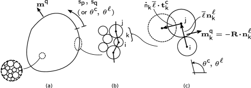
Figure 3: Boundary chain of particles for finding the velocity gradient: (a) bounded assembly of particles, (b) chain of boundary branch vectors, and (c) two boundary particles.

The area-average velocity gradient is

$$\mathbf{L} =\frac{1}{A}\iint\limits_{A}\frac{\partial v_{i}}{\partial x_{j}}\,dA$$ (29)

$$=\frac{1}{A}\int_{0}^{S}\int_{0}^{S}\frac{dv_{i}}{ds^{p}}\,Q\left(s^{p},s^{q}\right)m_{j}^{q}\,ds^{p}ds^{q}$$ (30)

where $S$ is the perimeter length; $\mathbf{m}^{q}$ is the unit outward normal of the perimeter at position $s^{q}$; $A$ is the enclosed area; $dv_{i}/ds^{p}$ is the derivative of the velocity component $v_{i}$ along the perimeter, as point $s^{p}$ traverses this boundary; and kernel $Q$ is a discontinuous function with domain $[0,S)$ and range $(-1/2,1/2)$ given by

$$Q\left(s^{p},s^{q}\right)=\begin{cases}\displaystyle\frac{1}{2}-\frac{1}{S}\operatorname{mod}\left(s^{q}-s^{p},S\right),&s^{q}\neq s^{p}\\ 0,&s^{q}=s^{p}\end{cases}$$ (31)

using the modulo $\text{mod}(\,)$ function. Integral (30) is an objective rate and requires only two types of information around the boundary: the boundary normal $\mathbf{m}^{q}$ and the relative motion $dv_{i}/ds^{p}$ along the perimeter, which is related to the contact motions. The enclosed area $A$ can also be expressed in a similar manner (Section 2.6). Equation (30) is a general and exact expression for the average spatial gradient within a closed two-dimensional region (bounded by a Jordan curve), provided that the boundary derivative $dv_{i}/ds$ is integrable and consistent with a field of boundary displacements, such that $\int_{0}^{S}(dv_{i}/ds)\,ds=0$.

For an assembly of disks, we focus on the closed polygonal chain of $M^{\text{per}}$ segments (branch vectors) formed by the contacting disks along the assembly’s perimeter (Fig. 3b). The perimeter segment $k$ between particles $i$ and $j$ has outward unit normal $\mathbf{m}^{q}_{k}$ which is perpendicular to the branch vector, $\mathbf{m}^{q}_{k}=-\mathbf{R}\cdot\mathbf{n}^{\ell}_{k}$, with arc length $\int_{i}^{j}ds^{q}=\overline{\ell}$ and rotation tensor $\mathbf{R}$ that effects a counterclockwise rotation of $\pi/2$:

$$\mathbf{R}=\begin{bmatrix}0&-1\\ 1&0\end{bmatrix}$$ (32)

In applying Eq. (30) to critical state flow, we assume that the particles are rigid and that bulk deformation is entirely due to the relative tangential motions between contacting particles. That is, we neglect any small changes in contact indentations during deformation and neglect the opening (extinction) and closing (creation) of contacts during small increments of bulk deformation. Such normal motions have a negligible contribution to the bulk deformation (characteristic A.1 in the Introduction). Considering only tangential motions, the velocity of particle $j$ relative to $i$ is equal to the angular rate $\dot{n}_{k}$ multiplied by branch length $\overline{\ell}$ and by the unit tangential direction $\mathbf{t}^{\text{c}}_{k}$, producing the rate vector $\dot{n}_{k}\overline{\ell}\,\mathbf{t}^{\text{c}}_{k}$ (Fig. 3c). This relative velocity occurs along a branch vector of length $\overline{\ell}$, so that derivative $dv_{i}/ds^{p}=\dot{n}_{k}\mathbf{t}^{\text{c}}_{k}$. Rate $\dot{n}_{k}$ can be expressed in terms of “$\phi$” rates (see Eq. 2), as

$$\dot{n}_{k}=\left.\left(2\dot{\phi}_{\text{slip},k}+\sqrt{2}\,\dot{\phi}_{\text{rigid},k}\right)\right/\sqrt{6}$$ (33)

The double integration in (30) distinguishes between “$p$” and “$q$” quantities: $s^{p}$ is associated with contact movement, whereas $s^{q}$ is associated with the outer normal $\mathbf{m}^{q}$. In a similar manner, we distinguish between the “c” and “$\ell$” directions, $\mathbf{t}^{\text{c}}_{k}$ and $\mathbf{n}^{\ell}_{k}$, and write (30) as the double sum:

$$\mathbf{L}=-\frac{\overline{\ell}^{2}}{A}\sum_{p=1}^{M^{\text{per}}}\sum_{q=1}^{M^{\text{per}}}\dot{n}_{p}\,Q\left(s^{p},s^{q}\right)\,\mathbf{t}^{\text{c}}_{p}\otimes\left(\mathbf{R}\cdot\mathbf{n}^{\ell}_{q}\right)$$ (34)

where $M^{\text{per}}$ is the number of perimeter contacts, and $s^{p}$ and $s^{q}$ are measured counterclockwise from a single, common perimeter point. This double sum is an exact expression for average strain in a mono-disperse assembly of disks, provided that contact movements are limited to tangential displacement.

To develop a corresponding function $\Gamma(\cdots)$ that can be integrated as in Eq. (7), we idealize the material region in the limit of a very large assembly of disks in which the perimeter chain of contacts has an orientation $\theta$ that increases monotonically from one contact to the next, forming a convex, nearly smooth boundary. In making this idealization, we neglect the non-convex “inside corners” that would typically occur around a polygonal loop of branch vectors. Arc distances $s^{p}$ and $s^{q}$ can now be approximately parameterized with angles $\theta^{\text{c}}$ and $\theta^{\ell}$. We also assume that the probability density of these angles is the same as that within the interior of the region: the density $p(\cdot,\cdot,\theta^{\text{c}},\theta^{\ell},\cdot,\cdot)$. The shape of the boundary chain will depend upon this density, which furnishes the relative numbers of contacts at different orientations. With these assumptions, Eqs. (30), (31), and (34) are written as

$$\mathbf{L}\approx\underset{(g^{\text{n}},g^{\text{t}},\theta^{\text{c}},\theta^{\ell},\dot{\phi}_{\text{slip}},\dot{\phi}_{\text{rigid}})}{\idotsint}\boldsymbol{\Gamma}_{\mathbf{L}}(\cdots)\,p(\cdots)$$ (35)

with function $\boldsymbol{\Gamma}_{\mathbf{L}}$ and kernel $K_{3}(\theta^{\text{c}},\theta^{\ell})$,

$$\boldsymbol{\Gamma}_{\mathbf{L}}(\cdots) =-\frac{\left(M^{\text{per}}\overline{\ell}\right)^{2}}{A}\,K_{3}(\theta^{\text{c}},\theta^{\ell})\,\dot{n}\,\mathbf{t}^{\text{c}}\otimes(\mathbf{R}\cdot\mathbf{n}^{\ell})$$ (36)

$$K_{3}(\theta^{\text{c}},\theta^{\ell}) =\begin{cases}\displaystyle\frac{1}{2}-\frac{1}{2\pi}\operatorname{mod}(\theta^{\ell}-\theta^{\text{c}},2\pi),&\theta^{\ell}\neq\theta^{\text{c}}\\ 0,&\theta^{\ell}=\theta^{\text{c}}\end{cases}$$ (37)

and with $\mathbf{n}^{\ell}$ and $\mathbf{R}$ defined in Eq. (32) and $\dot{n}$ defined in Eq. (33). Unlike the Dirac kernel ($K_{2}$ in Eq. 18), the kernel $K_{3}$ of Eq. (37) effects the double sum of Eq. (34), in which the two arguments ($\theta^{\text{c}}$ and $\theta^{\ell}$, or $s^{p}$ and $s^{q}$) correspond to different points on the assembly boundary.

Although Eqs. (30) and (34) yield exact average gradients, Eqs. (35)–(37) are an estimate. The author’s DEM simulations show errors of 5%–25% for disk assemblies in critical state flow. Notwithstanding the small error, the approximation (35) is only intended as a modest constraint on the contact motions, holding them to a nearly isochoric condition. Errors result from a number of sources: (1) the non-tangential (normal) contact movements that can occur between non-rigid grains; (2) the approximation of $ds$ in Eq. (30) with $M^{\text{per}}\overline{\ell}p(\cdots)d\theta$ in Eq. (35), which is a truncation of the full expansion of $s(\theta)$; (3) the non-monotonic variation of $\theta$ around a non-convex perimeter chain of branch vectors; and (4) subtle correlations among the branch vector lengths $\ell$, contact movements $\dot{n}$, and orientations $\theta^{\text{c}}$ and $\theta^{\ell}$.

The isochoric constraint on the probability density $p(\cdots)$ is the requirement of a zero expected value of trace $\text{tr}(\mathbf{L})$, expressed as

$$\begin{gathered}\left\langle\Gamma_{3}(\cdots)\right\rangle=\overline{\Gamma}_{3}\;\text{, where}\\ \Gamma_{3}(\cdots)=K_{3}(\theta^{\text{c}},\theta^{\ell})\operatorname{tr}\left[(\dot{n}\mathbf{t}^{\text{c}})\otimes(\mathbf{R}\cdot\mathbf{n}^{\ell})\right]\quad\text{and}\quad\overline{\Gamma}_{3}=0\end{gathered}$$ (38)

in which the leading constant term in (36) is canceled. The dyad in Eq. (38) is

$$\dot{n}\,\mathbf{t}^{\text{c}}\otimes(\mathbf{R}\cdot\mathbf{n}^{\ell})=K_{1}(\theta^{\text{c}})\,\dot{n}\begin{bmatrix}\sin\theta^{\text{c}}\sin\theta^{\ell}&-\sin\theta^{\text{c}}\cos\theta^{\ell}\\ -\cos\theta^{\text{c}}\sin\theta^{\ell}&\cos\theta^{\text{c}}\cos\theta^{\ell}\end{bmatrix}$$ (39)

with trace

$$\operatorname{tr}\left[\dot{n}\mathbf{t}^{\text{c}}\otimes(\mathbf{R}\cdot\mathbf{n}^{\ell})\right]=K_{1}\,(\theta^{\text{c}})\dot{n}\left(\sin\theta^{\text{c}}\sin\theta^{\ell}+\cos\theta^{\text{c}}\cos\theta^{\ell}\right)$$ (40)

where $\dot{n}$ is given by Eq. (33), and function $K_{1}(\theta^{\text{c}})$ of Eq. (15) enforces the biaxial symmetry shown in Fig. 2.

2.6 Fundamental constraint 4: Loading rate

We must specify the deformation rate $\dot{\varepsilon}$ that was included in the second (dissipation) constraint of Eqs. (27) and (28). Applying Eqs. (35) and (36) to the single deformation component $L_{11}=-\dot{\varepsilon}$ of Eq. (26) yields the following constraint on probability density $p(\cdots)$:

$$-\frac{\left(M^{\text{per}}\overline{\ell}\right)^{2}}{A}\underset{(g^{\text{n}},g^{\text{t}},\theta^{\text{c}},\theta^{\ell},\dot{\phi}_{\text{slip}},\dot{\phi}_{\text{rigid}})}{\idotsint}K_{3}(\theta^{\text{c}},\theta^{\ell})\,\dot{n}\,\left[\mathbf{t}^{\text{c}}\otimes(\mathbf{R}\cdot\mathbf{n}^{\ell})\right]_{,11}=-\dot{\varepsilon}$$ (41)

We can eliminate the leading coefficient $(M^{\text{per}}\overline{\ell})^{2}/A$ by again considering the deformation gradient of Eqs. (30), (35), and (36), but for the special case of an ideal dilation, with $dv_{1}/ds^{p}=n_{1}^{p}$ and $dv_{2}/ds^{p}=n_{2}^{p}$, which produces a known deformation rate with trace $\text{tr}(\mathbf{L})=2$:

$$-\frac{\left(M^{\text{per}}\overline{\ell}\right)^{2}}{A}\underset{(g^{\text{n}},g^{\text{t}},\theta^{\text{c}},\theta^{\ell},\dot{\phi}_{\text{slip}},\dot{\phi}_{\text{rigid}})}{\idotsint}K_{3}(\theta^{\text{c}},\theta^{\ell})\,\text{tr}\left(\mathbf{n}^{\text{c}}\otimes(\mathbf{R}\cdot\mathbf{n}^{\ell})\right)=2$$ (42)

Dividing Eq. (41) by Eq. (42) and rearranging terms gives the fourth constraint on density $p(\cdots)$:

$$\begin{gathered}\left\langle\Gamma_{4}(\cdots)\right\rangle=\overline{\Gamma}_{4}\;\text{, where}\\ \Gamma_{4}(\cdots)=K_{3}(\theta^{\text{c}},\theta^{\ell})\left\{\frac{\dot{\varepsilon}}{2}\,\text{tr}\left[\mathbf{n}^{\text{c}}\otimes(\mathbf{R}\cdot\mathbf{n}^{\ell})\right]+\dot{n}\left[\mathbf{t}^{\text{c}}\otimes(\mathbf{R}\cdot\mathbf{n}^{\ell})\right]_{,11}\right\}\\ \quad\text{and}\quad\overline{\Gamma}_{4}=0\end{gathered}$$ (43)

which formally asserts the compression rate $\mathbf{L}_{11}=-\dot{\varepsilon}$, assuring consistency of second and third constraints (Eqs. 27 and 38). The function $\Gamma_{4}(\cdots)$ is computed as

$$\Gamma_{4}(\cdots)=K_{3}(\theta^{\text{c}},\theta^{\ell})\left(\frac{\dot{\varepsilon}}{2}K_{1}(\theta^{\text{c}})(\sin\theta^{\text{c}}\cos\theta^{\ell}-\cos\theta^{\text{c}}\sin\theta^{\ell})+\dot{n}\sin\theta^{\text{c}}\sin\theta^{\ell}\right)$$ (44)

with $\dot{n}$ given by Eq. (33).

2.7 Auxiliary constraint 5: Fraction of sliding contacts

The four constraints given above describe a model of critical state flow under biaxial loading. Although a simple four-constraint model will predict nearly all trends observed in experiments and numerical simulations, the qualitative agreement is, in some respects, in poorer accord: in particular, it over-predicts the fraction of sliding contacts and the activity of contact movements (a prediction of over 80% sliding contacts). These aspects can be improved with the supply of new information to the model — information of an entirely empirical origin. We include a single modest parcel of information. A four-constraint model predicts an excess in the fraction of sliding contacts (more than 80%), compared with the much smaller values noted in characteristic C.1 of the Introduction. The final constraint limits the fraction of sliding contacts $\eta$:

$$\begin{gathered}\left\langle\Gamma_{5}(\cdots)\right\rangle=\overline{\Gamma}_{5}\;\text{, where}\\ \overline{\Gamma}_{5}=\eta\;\;\text{and}\\ \Gamma_{5}(\cdots)=\begin{cases}1,&g^{\text{t}}\in\{-\mu g^{\text{n}},\mu g^{\text{n}}\}\\ 0,&g^{\text{t}}\in(-\mu g^{\text{n}},\mu g^{\text{n}})\end{cases}\end{gathered}$$ (45)

where a value of $\eta$ is empirically derived.

2.8 Entropy

In the view of an experimentalist or simulator, a granular medium is a deterministic system — although one of bewildering complexity — in which the evolving conditions of each contact (its motions, forces, etc.) are uniquely determined by its own condition, by the conditions of all other contacts in the system, and by the boundary motions and forces. The probabilities $p(\cdots)$ are accessible, in this view, by frequent empirical observation of the contacts: from data in the form of the $M^{6}$ “$k$” values. Jaynes (1957) describes this as an “objective” approach to probability, when probability is an expressed expectation based on observation. To Jaynes, statistical mechanics is based upon an alternative “subjective” school of thought in which probabilities are simply expressions of expectation based upon general information that is usually very limited. Any shortcomings of such predictions, when compared with experimental observation, are attributed by the “subjectivist” not to insufficient acuity but to insufficient information. Indeed, to the subjectivist, the notion of probability is irrelevant when all information of a deterministic system is available beforehand: such an exercise is not one of prediction but of certitude.

From a subjective viewpoint, this lack of information is synonymous with uncertainty, disorder, or “entropy” and is quantified, in our case, with the differential Shannon entropy

$$H\left(p(\cdots)\right)=\!\underset{(g^{\text{n}},g^{\text{t}},\theta^{\text{c}},\theta^{\ell},\dot{\phi}_{\text{slip}},\dot{\phi}_{\text{rigid}})}{\idotsint}\!\!\!\!p(\cdots)\ln\left(p(\cdots)\right)$$ (46)

where $p(\cdots)$ must satisfy the constraints of the previous sections. Although restrictive, this small set of constraints does not, by itself, determine a unique macro-state, as many macro-states will satisfy the same constraints. The most likely macro-state — the most likely probability density $p(\cdots)$ — is the one that encompasses the greatest breadth of admissible micro-states among the $M^{6}$ space of possibilities (see Jaynes, 1957). For a large sample size (i.e. large $M$), this probability density maximizes $H$ while satisfying any available information that restricts the admissible micro-states: information in the form of our five moment constraints

$$\left\langle\Gamma_{i}(\cdots)\right\rangle=\overline{\Gamma}_{i},\quad i=1,2,\ldots,5$$ (47)

If, instead, a granular system was to settle upon a macro-state of lower entropy, this occurence would indicate a bias toward greater order (a macro-state with a smaller breadth of micro-states), suggesting an influence of other unaccounted information (i.e., other constraints). This possibility is addressed in the conclusions.

Following the Jaynes formalism of maximizing $H$ (i.e., the “MaxEnt” principle), the condition

$$\frac{\partial H(p(\cdots))}{\partial p(\cdots)}=0$$ (48)

and the zeroth constraint of Eq. (9) lead to the most likely density

$$p(\cdots)=\frac{1}{Z(\cdots)}\exp\left(-\sum_{i=1}^{5}\lambda_{i}\Gamma_{i}(\cdots)\right)$$ (49)

with normalizing (partition) function $Z$,

$$Z(\cdots)=\underset{(g^{\text{n}},g^{\text{t}},\theta^{\text{c}},\theta^{\ell},\dot{\phi}_{\text{slip}},\dot{\phi}_{\text{rigid}})}{\idotsint}\exp\left(-\sum_{i=1}^{5}\lambda_{i}\Gamma_{i}(\cdots)\right)$$ (50)

and with five Lagrange multipliers $\lambda_{i}$ that are computed so that the five moment constraints are satisfied (again, Jaynes, 1957). These multipliers are computed as the solutions of five non-linear equations, requiring a rather taxing evaluation of multiple multi-dimensional integrations, as described in B.

3 DEM Simulations and Model Verification

This section describes the small set of parameters that are required to implement and solve the model (Section 3.1), the DEM simulations that were used to evaluate the model (Section 3.2), and the results of this evaluation (Section 3.3).

3.1 Model implementation

The model requires three input parameters: the inter-particle friction coefficient $\mu$, the fraction of sliding contacts $\eta$, and the contact density coefficient $(M^{\text{int}}\overline{\ell}^{2}/A)^{-1}$. Mean stress $p_{\text{o}}$ and strain rate $\dot{\varepsilon}$ also appear, but only as scaling factors, and the forces and sliding rates are normalized with respect to these factors. Coefficient $(M^{\text{int}}\overline{\ell}^{2}/A)^{-1}$ is largely a scaling factor that does not significantly affect results and was was assigned a value of 1.5 in all calculations (see the end of Section 2.3). Results depend primarily on the friction coefficient, and a range of values were used ($\mu=0.1$, 0.3, 0.5, 0.7, and 0.9), with most results reported for $\mu=0.5$. The fraction $\eta$ ranged from 5% to 37% in the simulations, depending on friction $\mu$. An average value of 15% was used with the model.

Equations (47)–(50) define the density $p(\cdots)$ that corresponds to maximum disorder, a density expressed in terms of five multipliers $\lambda_{i}$. Once the $\lambda_{i}$ are computed (B), we can extract meaningful information from the model by evaluating various expected values and marginal distributions of $p(\cdots)$. These evaluations and an associated notational system are described in C.

3.2 DEM simulations

Statistics of contact force, movement, and orientation were gathered from simulations of 168 assemblies, each with 676 bi-disperse disks, which were sheared in horizontal biaxial compression. Details of the simulations are found in D. The bulk behavior is illustrated in Fig. 4, which shows the evolution of stress, fabric, and porosity. The Satake fabric tensor $F_{ij}$ is the average $\langle n_{i}^{\text{c}}n_{j}^{\text{c}}\rangle$ of the contact orientation vectors $\mathbf{n}^{\text{c}}$, and the ratio $F_{11}/F_{22}$ is a fundamental measure of bulk anisotropy (Satake, 1982).

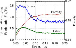
Figure 4: Stress, fabric, and porosity from DEM simulations (friction coefficient $\mu=0.50$).

A large initial stiffness causes the stress ratio $\sigma_{11}/\sigma_{22}$ to rise quickly from 1.0 to a peak condition at strain $-\varepsilon_{11}=2\%$, and the critical state condition is reached at compressive strains beyond 16–18%, with a mean value of ratio $\sigma_{11}/\sigma_{22}$ of 1.80. While in the critical state, the bulk response is seen to fluctuate (with a standard deviation of 0.03), indicating the agitated, tumultuous nature of the underlying particle interactions.

By running 168 simulations with random initial configurations and by taking several snapshots during the subsequent critical state flow, we collected over 800,000 contact samples of orientations, forces, and movements. Once the critical state is reached, we found that any bulk average of the micro-scale data (stress, fabric, density, etc.) or any marginal distribution thereof attains a nearly constant, steady condition.

3.3 Comparison of model and DEM results

The Introduction recounts numerous micro-scale characteristics of granular flow. We will find strong qualitative agreement with the DEM results: with most characteristics described in the Introduction, the model and simulations exhibit the same trends. In presenting the model results, the following paragraphs are preceded with raised items (e.g., “B.7”) that refer to particular characteristics in the Introduction, and the corresponding references to the literature can be found there. Primary predictions of the entropy model are shown in Table 3, with references to the Introduction shown as raised items in the first column. The third column in Table 3 defines the various quantities, using the notation of C. Only averages are reported, although dispersions from the mean can also be extracted with the model. Unless otherwise noted, the results of the model and the simulations are for the single case $\mu=0.50$.

In the following, the normal contact forces $g^{\text{n}}$ are divided by $2(M^{\text{int}}\overline{\ell}^{2}/A)^{-1}$ (i.e., the $\overline{\Gamma}_{2}$ factor in Eq. 20), so that the mean normed value $\langle g^{\text{n}}\rangle_{\text{normed}}$ is 1 (row 6 of Table 3). In terms of an actual force $f^{\text{n}}$, the normalized $g^{\text{n}}_{\text{normed}}$ equals $f^{\text{n}}(M^{\text{int}}\overline{\ell}/2p_{\text{o}}A)$.

Table 3: Results of DEM simulations and model (friction coefficient $\mu=0.50$). Raised items in the first column refer to characteristics in the Introduction.

			Values
	Description	Definition (see C)	DEM	Model
1${}^{\text{(B.1)}}$	Fabric tensor ratio, $F_{11}/F_{22}$	$\langle n_{1}n_{1}\rangle/\langle n_{2}n_{2}\rangle$	1.30	1.42
2${}^{\text{(B.2)}}$	Deviatoric stress ratio, $q/p_{\text{o}}$	$\langle\Gamma_{\sigma,11}-\Gamma_{\sigma,22}\rangle/p_{\text{o}}$	0.573	0.605
3${}^{\text{(B.3)}}$	Tangential force contribution to the deviatoric stress ratio, $q^{\text{t}}/p_{\text{o}}$	${}^{*\,}$$\alpha\langle g^{\text{t}}(n_{1}t_{1}-n_{2}t_{2})\rangle/p_{\text{o}}$	0.068	0.045
4${}^{\text{(B.3)}}$	Normal force contribution to the deviatoric stress ratio, $q^{\text{n}}/p_{\text{o}}$	${}^{*\,}$$\alpha\langle-g^{\text{n}}(n_{1}n_{1}-n_{2}n_{2})\rangle/p_{\text{o}}$	0.505	0.560
5${}^{\text{(B.3)}}$	Percent contribution of tangential forces to deviatoric stress	$q^{\text{t}}/q$	11.9%	7.5%
6	Mean normal contact force, normalized	$\langle g^{\text{n}}\rangle_{\text{normed}}$	1	1
7${}^{\text{(B.4)}}$	Fraction of deviator stress from weak contacts	$\langle\Gamma_{\sigma,11}-\Gamma_{\sigma,22}\rangle|_{g^{\text{n}}<1}$	7.2%	11.0%
8${}^{\text{(B.4)}}$	Fraction of mean stress from weak contacts	$\frac{1}{2}\langle\Gamma_{\sigma,11}+\Gamma_{\sigma,22}\rangle|_{g^{\text{n}}<1}$	28.7%	26.7%
9${}^{\text{(B.5)}}$	Fabric tensor ratio among weak contacts	$\langle n_{1}n_{1}\rangle|_{g^{\text{n}}<1}/\langle n_{2}n_{2}\rangle|_{g^{\text{n}}<1}$	1.05	1.17
10${}^{\text{(B.5)}}$	Fabric tensor ratio among strong contacts	$\langle n_{1}n_{1}\rangle|_{g^{\text{n}}>1}/\langle n_{2}n_{2}\rangle|_{g^{\text{n}}>1}$	1.76	1.80
11${}^{\text{(C.1)}}$	Fraction of sliding contacts, $\eta$	$\langle 1\rangle|_{g^{\text{t}}\in\{-\mu g^{\text{n}},\mu g^{\text{n}}\}}$	11.2%	15.0%
12${}^{\text{(B.6)}}$	Fraction of forward sliding contacts, $\eta^{+}$	$\langle 1\rangle|_{g^{\text{t}}=\mu g^{\text{n}}}$	6.6%	7.7%
13${}^{\text{(B.6)}}$	Fraction of reverse sliding contacts, $\eta^{-}$	$\langle 1\rangle|_{g^{\text{t}}=-\mu g^{\text{n}}}$	4.6%	7.3%
14${}^{\text{(B.6)}}$	Ratio of forward and reverse sliding contacts	$\eta^{+}/\eta^{-}$	1.43	1.05
15${}^{\text{(B.8)}}$	Mean normal contact force among non-sliding contacts	$\langle g^{\text{n}}|g^{\text{t}}\in(-\mu g^{\text{n}},\mu g^{\text{n}})\rangle_{\text{normed}}$	1.073	1.15
16${}^{\text{(B.8)}}$	Mean normal contact force among forward sliding contacts	$\langle g^{\text{n}}|g^{\text{t}}=\mu g^{\text{n}}\rangle_{\text{normed}}$	0.335	0.174
17${}^{\text{(B.8)}}$	Mean normal contact force among reverse sliding contacts	$\langle g^{\text{n}}|g^{\text{t}}=-\mu g^{\text{n}}\rangle_{\text{normed}}$	0.306	0.159
∗ $\alpha=M^{\text{int}}\overline{\ell}^{2}p_{\text{o}}/A$

${}^{(\text{B.1})}$As the most telling result, the model predicts an anisotropy of contact orientation that is consistent with the simulations: contacts are predominantly oriented in the direction of the major principal compressive stress, with a Satake fabric ratio $F_{11}/F_{22}=\langle n_{1}n_{1}\rangle/\langle n_{2}n_{2}\rangle$ that is greater than one (row 1 of Table 3). The distribution of contact orientations is shown in Fig. 5, in which the $[0,2\pi)$ range has been folded to $[0,\pi/2)$ in accordance with the biaxial symmetry of loading.

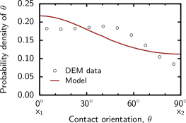
Figure 5: Density distribution of contact orientation for horizontal biaxial compression in the $x_{1}$ direction, $\mathcal{D}_{\theta^{\text{c}}}\langle 1\rangle$. Orientation $\theta=0$ corresponds to contact normals that are aligned with the compression direction ($x_{1}$ in Fig. 2).

In this and other figures, the $x_{1}$ direction (i.e., $\theta=0$) refers to contact normals that are oriented in the (horizontal) direction of compressive loading, and $x_{2}$ is in the direction of extension (Fig. 2). Although the model and simulations display some differences, the model correctly predicts the general trend of the orientation distribution.

${}^{(\text{B.2})}$The model predicts that stress in the compression direction, $-\sigma_{11}$, is larger than that in the extension direction, $-\sigma_{22}$, and the model predicts a deviator stress ratio, $q/p_{\text{o}}=-(\sigma_{11}-\sigma_{22})/p_{\text{o}}$ that is close to the value from the DEM simulations (Table 3, row 2). As in Eqs. (10), (16), and (17), deviatoric stress can result from three sources: from contact orientations biased in the compression direction, from larger normal contact forces in this same direction, and from the tangential contact forces. The predicted anisotropy of contact orientation was verified above (Fig. 5 and row 1). The model also predicts an anisotropy of the average normal forces, as is illustrated in Fig. 6a. The results of the simulations and model are similar: normal forces are, on average, larger in the direction of bulk compression.

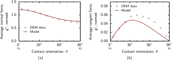
Figure 6: Average contact force as a function of contact orientation: (a) average normal contact force, $\langle g^{\text{n}}\rangle(\theta^{\text{c}})$, and (b) average tangential contact force, $\langle g^{\text{t}}\rangle(\theta^{\text{c}})$.

Anisotropy of tangential contact force is shown in Fig. 6b. For both simulations and model, the averaged tangential force is largest at an angle of about 40^∘ oblique to the compression direction. Although the numerical values of simulations and theory differ, the model captures the primary trend of anisotropy in the tangential force.

${}^{(\text{B.3})}$The separate contributions of the normal and tangential forces to the full deviatoric stress can be extracted with the model, as these contributions are proportional to the expected values $\langle-g^{\text{n}}(n_{1}n_{1}-n_{2}n_{2})\rangle$ and $\langle g^{\text{t}}(n_{1}t_{1}-n_{2}t_{2})\rangle$. For both simulations and model, the relative contribution of the tangential forces to the full deviator stress $q$ is minor: a 11.9% contribution in the simulations and 8.9% from the model (rows 3–5, Table 3).

${}^{(\text{B.11})}$The model gives a fairly good prediction of the probability density of normal contact forces, as seen in Fig. 7a.

Figure 7: Density distributions of contact force: (a) normal force distribution, $\mathcal{D}_{g^{\text{n}}}\langle 1\rangle$, and (b) distribution of the fraction of mobilized friction of tangential forces, $\mathcal{D}_{g^{\text{t}}/\mu g^{\text{n}}}\langle 1\rangle$.

The model predicts an exponential tail for large normal forces $g^{\text{n}}$ (although somewhat less steep than the DEM data), and it predicts a curved, flattened “shoulder”for normal forces $g^{\text{n}}$ less than 1.5. The model, however, does give a steep rise in the distribution for the smallest normal forces (those with $g^{\text{n}}<0.1$).

${}^{(\text{C.2})}$The model poorly predicts the density of the tangential contact forces (see the plot of $g^{\text{t}}/\mu g^{\text{n}}$ in Fig. 7b). When considering only the non-sliding contacts (with $|g^{\text{t}}|<\mu g^{\text{n}}$), the density of this ratio in the DEM simulations decreases with an increasing mobilized friction, consistent with experimental results (Majmudar et al., 2007). The model, however, gives a nearly uniform density for this same condition. This shortcoming is discussed in the conclusions.

${}^{(\text{B.4,B.5})}$Contacts with a normal force less than the mean force (weak contacts) are known to operate differently than those with a greater-than-mean normal force (strong contacts). The orientation distribution of weak contacts is known to be nearly isotropic, with only a small bias in the direction of loading. Consistent with the simulations, the model predicts a Satake fabric ratio for weak contacts of only slightly greater than one (Table 3, row 9); whereas the corresponding value for the strong contacts is 1.8 (row 10): that is, the contact anisotropy of all contacts (=1.42) is almost entirely attributed to the strong contacts. The deviatoric stress is also primarily attributed to the strong contacts: with the simulations and the model, 11% or less of the deviator stress $q$ is derived from the weak contacts (row 7). The same weak contacts have a more significant role in bearing the mean stress, as more than 26% of $p_{\text{o}}$ is attributed to these contacts (row 8). The model is consistent with the simulations in all of these trends.

${}^{(\text{B.6})}$The DEM simulations show that the directions of the contact movements do not always conform to those expected of an affine deformation field. As shown in Fig. 2, two particles oriented in the first quadrant would move in a conforming, “forward” direction if particle “$j$” moves upward and to the left over particle “$i$”. Although most contact slip does occur in this forward direction, the simulations show that about 40% of sliding contacts slip in the reverse direction (rows 12–13). The model predicts this same trend of a large fraction of contacts slipping in the reverse direction.

${}^{(\text{B.7})}$The likelihood that a contact is sliding depends upon its orientation and also upon the magnitude of its normal force. Figure 8a shows that contact slip is most likely among contacts with normals $\mathbf{n}_{k}$ that are oriented in the direction of extension (direction $x_{2}$ for the biaxial loading conditions of this study, Fig. 2).

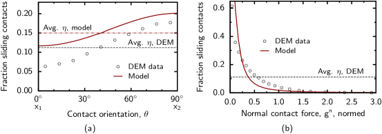
Figure 8: Fraction of sliding contacts as a function of (a) contact orientation, $\langle 1|g^{\text{t}}\in\{-\mu g^{\text{n}},\mu g^{\text{n}}\}\rangle(\theta^{\text{c}})$, and (b) normal contact force, $\langle 1|g^{\text{t}}\in\{-\mu g^{\text{n}},\mu g^{\text{n}}\}\rangle(g^{\text{n}})$.

Although the model’s results in 8a are shifted because of a different $\eta$ value, the same trend is predicted.

${}^{(\text{B.8})}$Figure 8b shows the relationship between the normal contact force $g^{\text{n}}$ and the fraction of sliding contacts. With both model and simulations, the prevalence of contact sliding decreases with an increasing contact force: contact slip is far more likely for lightly loaded contacts than for those bearing a large normal force. This trend is also captured by measuring the average normal forces among the sliding and non-sliding contacts (Table 3, rows 15–17): the average normal force among sliding contacts is less than a third of that among non-sliding contacts. Moreover, the normal force among forward sliding contacts is slightly greater than the force among contacts sliding in the reverse direction. All of these trends are predicted with the model.

${}^{(\text{B.7,B.9})}$The sliding (slip) rate $\dot{\phi}_{\text{slip}}$ also depends upon contact orientation (Fig. 9).

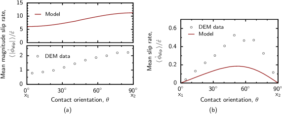
Figure 9: Sliding rate $\dot{\phi}_{\text{slip}}$ and contact orientation: (a) average magnitude of sliding rate, $\langle|\dot{\phi}_{\text{slip}}|/\dot{\varepsilon}\rangle(\theta^{\text{c}})$, and (b) mean sliding rate, $\langle\dot{\phi}_{\text{slip}}/\dot{\varepsilon}\rangle(\theta^{\text{c}})$.

As with the DEM data, the model predicts a more vigorous magnitude of the slip rate among contacts that are oriented in the direction of extension (Fig. 9a). Although the model is consistent with the DEM data in this trend, the magnitudes of the slip rate in the model are considerably greater than those of the simulations: the model greatly over-predicts the vigor of contact activity. Figure 9b shows the mean slip rate as a function of contact orientation. Consistent with the DEM data, the model predicts that the mean slip rate is, on average, in the “forward” (positive) direction and that the mean is largest at orientations oblique to the directions of compression and extension (at an angle of about 50^∘).

${}^{(\text{B.8})}$Figure 10 shows the relationship between the contact sliding rate and the contact normal force.

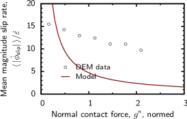
Figure 10: Sliding rate $\dot{\phi}_{\text{slip}}$ and contact normal force, $\langle|\dot{\phi}_{\text{slip}}|/\dot{\varepsilon}\rangle(g^{\text{n}})$.

Although quantitative agreement is poor, the simulations and the model show a reduction in the magnitude of slip movements with increasing normal force.

${}^{(\text{B.10})}$Past DEM analyses of strains within particle clusters have shown that dilation is associated with clusters that are elongated in the direction of compression; whereas, clusters that are elongated in the direction of extension tend to contract (Nguyen et al., 2009). With the model, this aspect of granular deformation was studied by extracting the dilation rate predicted when integration is restricted to different contact orientations $\theta^{\text{c}}$. The deformation function $\mathbf{\Gamma}_{\mathbf{L}}$ of Eq. (36) was analyzed with the methods of C (see Eq. 67) to compute the average dilation rate attributed to contacts of any given orientation $\theta^{\text{c}}$: the average $\langle\text{tr}(\mathbf{\Gamma}_{\mathbf{L}})/\dot{\varepsilon}\rangle(\theta^{\text{c}})$.

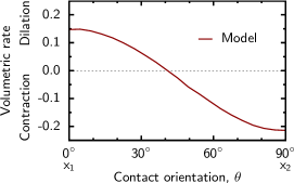
Figure 11: Average volumetric deformation rate attributed to contacts with orientation $\theta^{\text{c}}$: the expectation $\langle\text{tr}(\mathbf{\Gamma}_{\mathbf{L}})/\dot{\varepsilon}\rangle(\theta^{\text{c}})$.

Although the relationship between contact orientation and dilation was not computed for the current DEM simulations, the model results, shown in Fig. 11, do confirm past observations: contacts oriented in the direction of compression (direction $x_{1}$) are associated with the dilation of an assembly; whereas those oriented in the direction of extension tend to produce contraction.

${}^{(\text{B.12})}$As the final aspect of behavior, we consider the effect of the inter-particle friction coefficient $\mu$ on bulk strength at the critical state. DEM simulations were conducted with five coefficients and the model was solved with these same values. Figure 12 compares the model’s predictions of strength with the results of DEM simulations, expressed as the deviator stress ratio $q/p_{\text{o}}$.

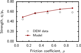
Figure 12: Effect of inter-particle friction coefficient $\mu$ on the deviatoric stress during critical state flow.

Although the model over-predicts strength at the critical state, its results follow a similar trend of the DEM data: strength increases with an increasing friction coefficient, but the increase is rather small for coefficients greater than 0.30.

4 Discussion

In the Introduction, we listed several micro-scale characteristics of critical state granular flow that have been observed in past experiments and simulations. These observations as well as new DEM simulations were used to evaluate a proposed model for granular flow. Nearly all of the model’s predictions are in qualitative (if not quantitative) agreement with observed characteristics. The model favorably predicts anisotropies of the contact orientations, contact forces, and contact movements and of the orientations of those contacts undergoing slip. The model also favorably predicts relationships between the contact force magnitude, contact motion, and contact slip direction. Although several pages were required for its derivation, and its solution requires quite demanding computations, the model’s concept is fairly simple: the contact landscape of motion, force, and orientation is maximally disordered at the critical state, after one accounts for the biases that arise from certain fundamental and empirical aspects of flow.

The model adopts individual contacts as its generic units, but without identifying their locations or their affiliations with other contacts. As such, it is certainly unable to resolve the spatial localization and meso-scale patterning that is usually found within granular flows (item D.1 in the Introduction). Past studies have shown that motions and forces are spatially coordinated (correlated) over distances of several particle diameters (Kuhn, 2003). Such patterning and correlation affirm a greater order (and lower entropy) than is accessible with the model.

Biased by the loading direction in the second constraint, the model predicts a maximally disordered condition that is anisotropic. Although anisotropy, by itself, connotes greater order than isotropy, the small increase in the order of contact orientation is more than offset by an increase in the disorder associated with the contact forces and movements.

In some respects, the model either poorly predicts behavior or requires an additional constraint to force agreement. These shortcomings include the density of the tangential contact forces among non-sliding contacts (Fig. 7b) and the fraction of sliding contacts (constraint 5). In other respects, the model is consistent with trends in the simulation results but is in poor quantitative agreement (for example, in the vigor of the contact movements, Fig. 9a). Although its successes are promising, the model’s shortcoming are more revealing, raising this question: why are some behaviors not amenable to a simple, contact-centric statistical treatment?

An underlying assumption of the Jaynes maximum entropy (MaxEnt) approach is that each micro-state is equally probable, provided that the micro-state is consistent with available information (i.e., the imposed constraints). In the current setting, each of the “$k$” micro-states $\{\cdots\}$ in the dimension-$M^{6}$ phase space belongs to a particular macro-state $(\cdots)$ and is assumed equiprobable with the other micro-states that populate the same macro-state. In the model, the micro-states only incorporate contact information and are devoid of content on the particles’ locations or their topologic arrangement. The equiprobable assumption ignores the fundamental meso-scale restrictions that are shared by the particles and contacts: the contact forces on each particle must be in equilibrium, and the contact movements must be compatible with a corresponding set of particle movements and rotations. These additional restrictions operate at a meso-scale much larger than individual contacts, and will bias some micro-states and disallow others altogether, creating an uneven landscape of the dimension-$M^{6}$ phase space of micro-states. For example, without the rather coersive restriction on the fraction of sliding contacts (constraint 5), the model predicts a fraction greater than 80%, rather than the 11.2% measured in the simulations. This result suggests that particle motions are coordinated (ordered) in a manner that greatly reduces the population of sliding contacts. Reasoning of a fundamental nature, applied to meso-scale conditions, is palpably needed to replace brute force, empirical constraints, such as our constraint on the fraction of sliding contacts and other constraints that are approximate in nature (constraints 3 and 4). We consider the lack of meso-scale information the primary deficiency of the model, and a means of introducing such information is suggested in the following paragraphs. On the other hand, those micro-scale characteristics and trends that are favorably predicted are apparently insensitive to meso-scale equilibrium and compatibility limitations, but are instead determined (or biased) by the rather broad constraints of pressure, of dissipation consistency, and of the isochoric condition.

The paper makes exclusive use of information that is formulated as moment constraints on the density $p(\cdots)$ (Eqs. 7 and 8). An alternative form of information was introduced by the author in a paper on topologic entropy (Kuhn, 2014). In this work, a relative entropy principle (cross-entropy or Kullback-Leibler entropy) was applied, admitting information in the form of certain a priori inclinations (priors) of $p(\cdots)$. Because these inclinations can have either an empirical or theoretical origin, this approach allows information — even imperfect information — gained from one theory (for example, an affine field approach) to be included in a shear-driven entropy model.

We should also consider the entropy model in relation to mean-field upscaling models, which have been used with reasonable success in estimating the small-strain stiffness of dense granular materials. These models can be more descriptive than predictive, as they require extensive additional information, in the form of contact stiffnesses, packing data, etc. Mean-field models, however, do provide a clearer, deterministic connection between the micro-scale and bulk behaviors: the micro and macro behaviors are unambiguously linked through contact rules. The corresponding connection is rather opaque in the paper’s approach. For example, why do the constraints lead to a greater number of forward sliding contacts than reverse sliding contacts? What features of the model lead to smaller normal forces among sliding contacts than for non-sliding contacts? Although the model yields some convincing predictions, the model is certainly enigmatic in regard to its results, as the model’s predictions are extracted only through a painstaking integration of distribution averages.

Finally, we suggest future extensions of this work. With some difficulty, the model could certainly be extended to three dimensions, which would require that the tangential forces and motions be expressed with Euler angles rather than the single $\theta$ orientation of the paper’s two-dimensional setting. The model could also be modified for non-circular or non-spherical particles, by allowing different orientations of the contacts and the branch vectors, $\theta^{\text{c}}$ and $\theta^{\ell}$ (i.e., by relaxing the Dirac restriction). In the Introduction, we had noted that granular materials consistently converge toward the critical state when loaded from differing initial conditions. Although the current model addresses the terminal condition at the critical state, the disorder in the paper’s contact quantitites (and other quantities, as well) could be tracked during the evolving condition of granular loading. An ideal entropy measure would increase in a consistent, monotonic manner during the loading process. This approach might lead to an improved entropy definition based upon a more appropriate phase space.

Dedication

The paper is dedicated to the memory of Dr. Masao Satake (1927–2013), who made significant fundamental contributions to granular mechanics.

Appendix A Integrations

Each constraint involves integrating a product $\Gamma_{i}(\cdots)p(\cdots)$, as sketched in Eq. (7). Any evaluation of these integrals must, in practice, reconcile the non-smooth nature of these integrands: both the rigid-frictional constitutive constraint of Eq. (4) and the kernel $K_{1}()$ are discontinuous. In the dimension-6 phase space, large non-zero values of $\dot{\phi}_{\text{slip}}$ can exist alongside an enforced zero value at the juncture of sliding and non-sliding behaviors: at hyper-planes $g^{\text{t}}=\pm\mu g^{\text{n}}$. This difficulty is resolved by splitting the original integral into three parts, so that each part addresses a single branch of the three constitutive cases in Eq. (4):

$$\underset{(g^{\text{n}},g^{\text{t}},\theta^{\text{c}},\theta^{\ell},\dot{\phi}_{\text{slip}},\dot{\phi}_{\text{rigid}})}{\idotsint}= \quad\underset{\begin{subarray}{c}\mathbb{R}^{+}\\ g^{\text{n}}\end{subarray}}{\int}\;\underset{\begin{subarray}{c}[0,\,2\pi)\\ \theta^{\text{c}}\end{subarray}}{\int}\;\underset{\begin{subarray}{c}[0,\,2\pi)\\ \theta^{\ell}\end{subarray}}{\int}\;\underset{\begin{subarray}{c}\mathbb{R}^{-}\\ \dot{\phi}_{\text{slip}}\end{subarray}}{\int}\;\underset{\begin{subarray}{c}\mathbb{R}\\ \dot{\phi}_{\text{rigid}}\end{subarray}}{\int}\;\begin{array}[]{l}\text{ with }g^{\text{t}}=-\mu g^{\text{n}}\\ \text{ and }\dot{\phi}_{\text{slip}}<0\end{array}$$ (53)

$$\quad+\underset{\begin{subarray}{c}\mathbb{R}^{+}\\ g^{\text{n}}\end{subarray}}{\int}\;\underset{\begin{subarray}{c}(-1,1)\\ g^{\text{t}}\end{subarray}}{\int}\;\underset{\begin{subarray}{c}[0,\,2\pi)\\ \theta^{\text{c}}\end{subarray}}{\int}\;\underset{\begin{subarray}{c}[0,\,2\pi)\\ \theta^{\ell}\end{subarray}}{\int}\;\underset{\begin{subarray}{c}\mathbb{R}\\ \dot{\phi}_{\text{rigid}}\end{subarray}}{\int}\begin{array}[]{l}\text{ with }g^{\text{t}}\in(-\mu g^{\text{n}},\mu g^{\text{n}})\\ \text{ and }\dot{\phi}_{\text{slip}}=0\end{array}$$ (56)

$$\quad+\underset{\begin{subarray}{c}\mathbb{R}^{+}\\ g^{\text{n}}\end{subarray}}{\int}\;\underset{\begin{subarray}{c}[0,\,2\pi)\\ \theta^{\text{c}}\end{subarray}}{\int}\;\underset{\begin{subarray}{c}[0,\,2\pi)\\ \theta^{\ell}\end{subarray}}{\int}\;\underset{\begin{subarray}{c}\mathbb{R}^{+}\\ \dot{\phi}_{\text{slip}}\end{subarray}}{\int}\;\underset{\begin{subarray}{c}\mathbb{R}\\ \dot{\phi}_{\text{rigid}}\end{subarray}}{\int}\;\begin{array}[]{l}\text{ with }g^{\text{t}}=\mu g^{\text{n}}\\ \text{ and }\dot{\phi}_{\text{slip}}>0\end{array}$$ (59)

The second integral on the right addresses the non-sliding branch, and the first and third integrals address sliding in the “reverse” and “forward” directions (sliding directions that are contrary to and consistent with those of affine deformation, as described in Section 2.1). Note that the three integrals are 5-fold, compared with the original 6-fold integrals (on the left of Eq. 53), greatly reducing the complexity of numerical evaluations. Separating (53) as three integrals also permits a direct application of constraint 5 (Eq. 45) and aids in computing separate statistics for the non-sliding and sliding (both forward and reverse) contacts (Section 3.3).

Appendix B Entropy numerics

The entropy $H$ in Eqs. (46)–(50) is maximized by finding the five multipliers $\lambda_{i}$ that satisfy the constraints $\langle\Gamma_{i}(\cdots)\rangle=\overline{\Gamma}_{i}$ of Eq. 8. That is, the proper $\lambda_{i}$ are the roots of five equations

$$f_{i}(\boldsymbol{\lambda})=A_{i}(\boldsymbol{\lambda})-\overline{\Gamma}_{i}Z(\boldsymbol{\lambda})=0$$ (60)

where argument $\boldsymbol{\lambda}$ represents the list $\{\lambda_{1},\lambda_{2},\ldots,\lambda_{5}\}$, and

$$A_{i}(\boldsymbol{\lambda})=\underset{(g^{\text{n}},g^{\text{t}},\theta^{\text{c}},\theta^{\ell},\dot{\phi}_{\text{slip}},\dot{\phi}_{\text{rigid}})}{\idotsint}\Gamma_{i}(\cdots)\exp\left(-\sum_{j=1}^{5}\lambda_{j}\Gamma_{j}(\cdots)\right)$$ (61)

We used the minpack library to solve these equations by minimizing the sum of their squared residuals (specifically, function hybrj1, which applies the Powell hybrid method) (Moré et al., 1984). The solver requires evaluation of the partition function $Z(\boldsymbol{\lambda})$, the five functions $f_{i}(\boldsymbol{\lambda})$, and the $5\times 5$ Jacobian

$$\frac{\partial f_{i}}{\partial\lambda_{j}} =-B_{ij}+\overline{\Gamma}_{i}A_{j}$$ (62)

$$B_{ij} =\underset{(g^{\text{n}},g^{\text{t}},\theta^{\text{c}},\theta^{\ell},\dot{\phi}_{\text{slip}},\dot{\phi}_{\text{rigid}})}{\idotsint}\Gamma_{i}(\cdots)\Gamma_{j}(\cdots)\exp\left(-\sum_{k=1}^{5}\lambda_{k}\Gamma_{k}(\cdots)\right)$$ (63)

The total of $1+5+25=31$ integrands were evaluated within each iteration of the solver hybrj1. Each symbolic integral is itself the sum of three integrals, each 5-fold (see Eq. 53). All integrals were evaluated with the CUBA library (specifically the function llcuhre, which applies adaptive polynomial cubature rules and permits a vector of integrands to be evaluated with each call). Except for the variables $g^{\text{t}}$, $\theta^{\text{c}}$, and $\theta^{\ell}$, which have ranges of $[-\mu g^{\text{n}},\mu g^{\text{n}}]$ or $[0,2\pi)$, all integrations are improper with infinite range. A change of variable, for example $u=\tan^{-1}g^{\text{n}}$, was applied in such cases, and integrations were evaluated with the following support: $g^{\text{n}}\in[0,10]$, $\dot{\phi}_{\text{slip}}\in[-200,200]$, and $\dot{\phi}_{\text{rigid}}\in[-200,200]$. Two hundred million points were queried in evaluating each integrand within each of the three integrals within each iteration. The mean stress $p_{\text{o}}$ and strain rate $\dot{\varepsilon}$ were both set to 1.0, and the factor $M^{\text{int}}\overline{\ell}^{2}/A$ was 1.50.

After solving the multipliers $\lambda_{i}$, meaningful results, such as those in Section 3.3 must be extracted by evaluating integrals with appropriate integrands to compute the relevant $\langle\cdot\rangle$ quantities. These calculations are described in the next appendix.

Appendix C Statistical calculations and notation

After determining the multipliers $\lambda_{i}$, meaningful information can be extracted from the probability density $p(\cdots)$ by post-processing of various integrals in the form of Eq. (53). Statistical notations used in the paper are intended to suggest their numerical evaluation, although some differ from traditional notations. The expected value of a function $h(\cdots)$ is written as $\langle h(\cdots)\rangle$ or $\langle h\rangle$ and is computed, as in Eqs. (7) and (53), by integrating across the full domain $(g^{\text{n}},g^{\text{t}},\theta^{\text{c}},\theta^{\ell},\dot{\phi}_{\text{slip}},\dot{\phi}_{\text{rigid}})$. When the domain is restricted by a condition $\Psi$, we use the notation $\langle h(\cdots)\rangle|_{\Psi}$,

$$\langle h(\cdots)\rangle\,|_{\Psi}=\left.\underset{(g^{\text{n}},g^{\text{t}},\theta^{\text{c}},\theta^{\ell},\dot{\phi}_{\text{slip}},\dot{\phi}_{\text{rigid}})}{\idotsint}\!\!\!\!\!h(\cdots)\,p(\cdots)\right|_{\Psi}$$ (64)

in which the integrand is zero outside of this restricted domain (i.e., where condition $\Psi$ is not met). For example, the probability of condition $\Psi$ is simply $\langle 1\rangle|_{\Psi}$, with $h=1$. The conditional expectation of function $h(\cdots)$ subject to $\Psi$ is written as $\langle h(\cdots)|\Psi\rangle$ and is computed as

$$\langle h(\cdots)|\Psi\rangle=\frac{\langle h(\cdots)\rangle|_{\Psi}}{\langle 1\rangle|_{\Psi}}$$ (65)

We also compare the statistics of contacts that are not sliding or are sliding in the “reverse” or “forward” directions. The three cases correspond to different $\Psi$ conditions: $\dot{\phi}_{\text{slip}}=0$, $\dot{\phi}_{\text{slip}}=<0$, and $\dot{\phi}_{\text{slip}}=>0$ (or alternatively, $g^{\text{t}}\in(-\mu g^{\text{n}},\mu g^{\text{n}})$, $g^{\text{t}}=-\mu g^{\text{n}}$, and $g^{\text{t}}=\mu g^{\text{n}}$), as explicitly isolated with the three integrals in Eq. (53).

The marginal probability density of a single contact quantity will be written as a derivative, in keeping with the manner in which it is computed. For example, the marginal probability density of the contact orientation $\theta^{\text{c}}$ is written as the derivative $\mathcal{D}_{\theta^{\text{c}}}\langle 1\rangle$:

$$\mathcal{D}_{\theta^{\text{c}}}\langle 1\rangle=\underset{\Delta\theta\rightarrow 0}{\lim}\frac{\langle 1\rangle|_{\theta^{\text{c}}<\theta<\theta^{\text{c}}+\Delta\theta}}{\Delta\theta}$$ (66)

As another example, the average expected normal force $g^{\text{n}}$ as a function of contact orientation $\theta^{\text{c}}$ is written and computed as

$$\langle g^{\text{n}}\rangle(\theta^{\text{c}})=\frac{\mathcal{D}_{\theta^{\text{c}}}\langle g^{\text{n}}\rangle}{\mathcal{D}_{\theta^{\text{c}}}\langle 1\rangle}=\underset{\Delta\theta\rightarrow 0}{\lim}\frac{\langle g^{\text{n}}\rangle|_{\theta^{\text{c}}<\theta<\theta^{\text{c}}+\Delta\theta}}{\langle 1\rangle|_{\theta^{\text{c}}<\theta<\theta^{\text{c}}+\Delta\theta}}$$ (67)

Appendix D DEM simulations, continued

Multiple discrete element (DEM) simulations of biaxial compression were conducted on bi-disperse assemblies of 676 particles. The two disk varieties have ratios of 1.5:1 in size, 1:2.25 in number, and 1:1 in cumulative area (that is, 468 particles of size $1.0$ and 208 of size $1.5$). The assemblies were small enough to prevent gross non-homogeneity in the form shear bands (no bands were observed, by using the methods of Kuhn, 1999), yet large enough to capture the average, bulk material behavior. To develop more robust statistics, 168 different assemblies were created by compacting random sparse frictionless mixtures of the two disk sizes into dense isotropic packings within periodic boundaries until the average contact indentation was $0.0002$ times the average radius. In the subsequent biaxial loading sequences, linear contact stiffnesses were applied between particles with equal tangential and normal coefficients ($k^{\text{t}}=k^{\text{n}}$), and the base friction coefficient $\mu=0.5$ was enforced during the pair-wise particle interactions (da Cruz et al., 2005). Coefficients $\mu=0.1$, 0.3, 0.7, and 0.9 were used in separate simulations, all starting from the same 168 assemblies. Using the standard DEM algorithm, the initially square assemblies were horizontally compressed in increments $\Delta\epsilon_{11}=1\times 10^{-6}$ while maintaining a constant mean stress of $2\times 10^{-4}k^{\text{n}}$ (Cundall and Strack, 1979). The strain rate was sufficiently slow to maintain the quasi-static condition, with the inertial number $I$ equal to $2.5\times 10^{-4}$ (i.e., the ratio of the shear time $1/\dot{\varepsilon}$ to the inertial time of a particle $\sqrt{m/p_{\text{o}}}$, see da Cruz et al., 2005). These loading conditions coincide with those described in Sections 2.5–2.6 and result in the stress, fabric, and volumetric behavior that are shown in Fig. 4. A large initial stiffness causes the deviatoric stress to rise quickly from zero to a peak stress at strain $-\varepsilon_{11}=2\%$, and the critical state condition is attained at compressive strains $-\varepsilon_{11}$ of 16–18%. During subsequent steady-state deformation, the contact conditions were interrogated at five strains between $-\varepsilon_{11}=16\%$ and $25\%$ (Fig. 4), and rates $\dot{n}$ and $\dot{\phi}$ were determined with pairs of interrogations separated by strain $\Delta\varepsilon_{11}=1\times 10^{-5}$. Applying the ergodicity principle, micro-state statistics were averaged across the five strains and the 168 assemblies, involving 840 pairs of interrogations containing about 820,000 contacts. Another series of simulations were run with poly-disperse assemblies having particle sizes spanning a range of 3.0. The results were similar to those of the bi-disperse assemblies, and only the latter are reported herein.

References

References

- Bagi (2006) Bagi, K., 2006. Analysis of microstructural strain tensors for granular assemblies. Int. J. Solids Struct. 43 (10), 3166–3184.
- Blumenfeld and Edwards (2009) Blumenfeld, R., Edwards, S. F., 2009. On granular stress statistics: Compactivity, angoricity, and some open issues. The Journal of Physical Chemistry B 113 (12), 3981–3987.
- Brown (2000) Brown, C. B., 2000. Entropy and granular materials: model. J. Eng. Mech. 126 (6), 599–604.
- Brown et al. (2000) Brown, C. B., Elms, D. G., Hanson, M. T., Nikzad, K., Worden, R. E., 2000. Entropy and granular materials: experiments. J. Eng. Mech. 126 (6), 605–610.
- Chakraborty (2010) Chakraborty, B., 2010. Statistical ensemble approach to stress transmission in granular packings. Soft Matt. 6 (13), 2884–2893.
- Cundall and Strack (1979) Cundall, P. A., Strack, O. D. L., 1979. A discrete numerical model for granular assemblies. Géotechnique 29 (1), 47–65.
- da Cruz et al. (2005) da Cruz, F., Emam, S., Prochnow, M., Roux, J.-N., Chevoir, F., 2005. Rheophysics of dense granular materials: Discrete simulation of plane shear flows. Phys. Rev. E 72 (2), 021309.
- Desrues and Viggiani (2004) Desrues, J., Viggiani, G., 2004. Strain localization in sand: an overview of the experimental results obtained in Grenoble using stereophotogrammetry. Int. J. Numer. and Anal. Methods in Geomech. 28, 279–321.
- Goddard (2004) Goddard, J. D., 2004. On entropy estimates of contact forces in static granular assemblies. Int. J. Solids Struct. 41 (21), 5851–5861.
- Härtl and Ooi (2008) Härtl, J., Ooi, J. Y., 2008. Experiments and simulations of direct shear tests: porosity, contact friction and bulk friction. Granul. Matter 10 (4), 263–271.
- Jaynes (1957) Jaynes, E. T., 1957. Information theory and statistical mechanics. Phys. Rev. 106 (4), 620–630.
- Jenkins and Strack (1993) Jenkins, J. T., Strack, O. D. L., 1993. Mean-field inelastic behavior of random arrays of identical spheres. Mech. of Mater. 16 (1), 25–33.
- Kruyt and Antony (2007) Kruyt, N. P., Antony, S. J., 2007. Force, relative-displacement, and work networks in granular materials subjected to quasistatic deformation. Phys. Rev. E 75 (5), 051308.
- Kruyt and Rothenburg (2014) Kruyt, N. P., Rothenburg, L., 2014. On micromechanical characteristics of the critical state of two-dimensional granular materials. Acta Mechanica 225 (8), 2301–2318.
- Kuhn (1999) Kuhn, M. R., 1999. Structured deformation in granular materials. Mech. of Mater. 31 (6), 407–429.
- Kuhn (2003) Kuhn, M. R., 2003. Heterogeneity and patterning in the quasi-static behavior of granular materials. Granul. Matter 4 (4), 155–166.
- Kuhn (2004a) Kuhn, M. R., 2004a. Boundary integral for gradient averaging in two dimensions: application to polygonal regions in granular materials. Int. J. Numer. Methods Eng. 59 (4), 559–576.
- Kuhn (2004b) Kuhn, M. R., 2004b. Rates of stress in dense unbonded frictional materials during slow loading. In: Antony, S. J., Hoyle, W., Ding, Y. (Eds.), Advances in Granular Materials: Fundamentals and Applications. Royal Society of Chemistry, London, U.K., pp. 1–28.
- Kuhn (2014) Kuhn, M. R., 2014. Dense granular flow at the critical state: maximum entropy and topological disorder. Granul. Matter 16 (4), 499–508.
- Kuhn and Bagi (2004) Kuhn, M. R., Bagi, K., 2004. Contact rolling and deformation in granular media. Int. J. Solids Struct. 41 (21), 5793–5820.
- Kuhn and Bagi (2005) Kuhn, M. R., Bagi, K., 2005. On the relative motions of two rigid bodies at a compliant contact: application to granular media. Mech. Res. Comm. 32 (4), 463–480.
- Liao et al. (1997) Liao, C.-L., Chang, T.-P., Young, D.-H., 1997. Stress-strain relationship for granular materials based on the hypothesis of best fit. Int. J. Solids Struct. 34 (31–32), 4087–4100.
- Majmudar and Bhehringer (2005) Majmudar, T. S., Bhehringer, R. P., 2005. Contact force measurements and stress-induced anisotropy in granular materials. Nature 435 (1079), 1079–1082.
- Majmudar et al. (2007) Majmudar, T. S., Sperl, M., Luding, S., Behringer, R. P., 2007. Jamming transition in granular systems. Phys. Rev. Lett. 98 (5), 058001.
- Moré et al. (1984) Moré, J. J., Sorensen, D. C., Hillstrom, K. E., Garbow, B. S., 1984. The MINPACK project. In: Cowell, W. R. (Ed.), Sources and Development of Mathematical Software. Prentice-Hall, Englewood Cliffs, N.J., pp. 88–111.
- Nguyen et al. (2009) Nguyen, N.-S., Magoariec, H., Cambou, B., Danescu, A., 2009. Analysis of structure and strain at the meso-scale in 2d granular materials. Int. J. Solids Struct. 46 (17), 3257–3271.
- Peña et al. (2008) Peña, A. A., Lizcano, A., Alonso-Marroquin, F., Herrmann, H. J., 2008. Biaxial test simulations using a packing of polygonal particles. Int. J. Numer. and Anal. Methods in Geomech. 32 (2), 143–160.
- Radjai et al. (1998) Radjai, F., Wolf, D. E., Jean, M., Moreau, J.-J., 1998. Bimodal character of stress transmission in granular packings. Phys. Rev. Lett. 80 (1), 61–64.
- Rothenburg (1980) Rothenburg, L., 1980. Micromechanics of idealized granular systems. Ph.D. thesis, Carleton University, Ottawa, Ontario, Canada.
- Rothenburg and Bathurst (1989) Rothenburg, L., Bathurst, R., 1989. Analytical study of induced anisotropy in idealized granular materials. Géotechnique 39 (4), 601–614.
- Rothenburg and Kruyt (2009) Rothenburg, L., Kruyt, N. P., 2009. Micromechanical definition of an entropy for quasi-static deformation of granular materials. J. Mech. Phys. Solids 57 (3), 634–655.
- Satake (1982) Satake, M., 1982. Fabric tensor in granular materials. In: Vermeer, P. A., Luger, H. J. (Eds.), Proc. IUTAM Symp. on Deformation and Failure of Granular Materials. A.A. Balkema, Rotterdam, pp. 63–68.
- Schofield and Wroth (1968) Schofield, A. N., Wroth, P., 1968. Critical state soil mechanics. McGraw-Hill, New York.
- Shannon (1948) Shannon, C. E., 1948. A mathematical theory of communication. Bell System Technical Journal 27 (3), 379–423.
- Thornton (2000) Thornton, C., 2000. Numerical simulations of deviatoric shear deformation of granular media. Géotechnique 50 (1), 43–53.
- Tordesillas et al. (2011) Tordesillas, A., Lin, Q., Zhang, J., Behringer, R. P., Shi, J., 2011. Structural stability and jamming of self-organized cluster conformations in dense granular materials. J. Mech. Phys. Solids 59 (2), 265–296.
- Troadec et al. (2002) Troadec, H., Radjai, F., Roux, S., Charmet, J. C., 2002. Model for granular texture with steric exclusion. Phys. Rev. E 66, 041305.
- Williams and Nabha (1997) Williams, J. R., Nabha, R., 1997. Coherent vortex structures in deforming granular materials. Mech. Cohesive-Frict. Mater. 2 (3), 223–236.
- Yoon and Giménez (2012) Yoon, S. W., Giménez, D., 2012. Entropy characterization of soil pore systems derived from soil-water retention curves. Soil Sci. 177 (6), 361–368.
- Zhao and Guo (2013) Zhao, J., Guo, N., 2013. A new definition on critical state of granular media accounting for fabric anisotropy. In: AIP Conference Proceedings. Vol. 1542. pp. 229–232.