Brown-HET-1781

4D, $\mathcal{N}=1$ Matter Gravitino Genomics

S.-N. Hazel Mak and Kory Stiffler

Department of Physics, Brown University,
Box 1843, 182 Hope Street, Providence, RI 02912, USA

ABSTRACT

Adinkras are graphs that encode a supersymmetric representation’s transformation laws that have been reduced to one dimension, that of time. A goal of the supersymmetry “genomics” project is to classify all 4D, $\mathcal{N}=1$ off-shell supermultiplets in terms of their adinkras. In previous works, the genomics project uncovered two fundamental isomer adinkras, the cis- and trans-adinkras, into which all multiplets investigated to date can be decomposed. The number of cis- and trans-adinkras describing a given multiplet define the isomer-equivalence class to which the multiplet belongs. A further refining classification is that of a supersymmetric multiplet’s holoraumy: the commutator of the supercharges acting on the representation. The one-dimensionally reduced, matrix representation of a multiplet’s holoraumy defines the multiplet’s holoraumy-equivalence class. Together, a multiplet’s isomer-equivalence and holoraumy-equivalence classes are two of the main characteristics used to distinguish the adinkras associated with different supersymmetry multiplets in higher dimensions. This paper focuses on two matter gravitino formulations, each with 20 bosonic and 20 fermionic off-shell degrees of freedom, analyzes them in terms of their isomer- and holoraumy-equivalence classes, and compares with non-minimal supergravity which is also a $20~{}\times~{}20$ multiplet. This analysis fills a missing piece in the supersymmetry genomics project, as now the isomer-equivalence and holoraumy-equivalence for representations up to spin two in component fields have been analyzed for 4D, $\mathcal{N}=1$ supersymmetry. To handle the calculations of this research effort, we have used the a Mathematica software package called Adinkra.m. This package is open-source and available for download at a GitHub Repository. Data files associated with this paper are also published open-source at a Data Repository also on GitHub.

PACS: 11.30.Pb, 12.60.Jv
Keywords: quantum mechanics, supersymmetry, off-shell supermultiplets

1 Introduction

Generally, there are more representations of supersymmetry (SUSY) in lower dimensions than there are in higher dimensions. Given a particular higher dimensional SUSY representation, one can always reduce the representation to lower dimension simply by considering the fields of the multiplet to depend only on the subset of coordinates required. For instance, in efforts known as “supersymmetric genomics”  [?,?,?], a 4D SUSY multiplet is reduced to 1D by considering the fields in the multiplet to depend only on time $\tau$. This is known as reducing to the 0-brane and the transformation laws for the 4D, $\mathcal{N}=1$ chiral multiplet, for instance, when reduced to the 0-brane can be entirely encoded in a graph known as an adinkra  [?,?,?,?,?,?,?,?], as shown in Figure 1. The precise meaning of the lines in the adinkra diagram are described in Section 2. Adinkras have been and continue to be used to discover new representations of supersymmetry: the 4D, $\mathcal{N}=2$ off-shell relaxed extended tensor mutliplet  [?] and a finite representation of the hypermultiplet  [?], for instance.

Figure 1: An adinkra for the 0-brane reduced transformation laws of the 4D, $\mathcal{N}=1$ chiral multiplet.

In previous supersymmetric genomics works  [?,?,?], the authors found adinkra representations for the 4D, $\mathcal{N}=1$ chiral multiplet (CM), vector multiplet (VM), tensor multiplet (TM), complex linear superfield multiplet (CLS), old-minimal supergravity (mSG), non-minimal supergravity ($\not$mSG), and conformal supergravity (cSG). They found these representations to decompose into a number $n_{c}$ of fundamental cis-adinkras and a number $n_{t}$ of trans-adinkras, as shown in Figure 2 and tabulated in Table 1 where $\chi_{0}=n_{c}-n_{t}$.

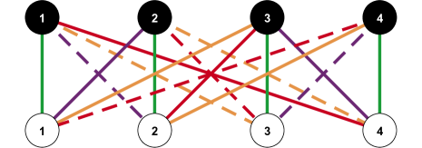
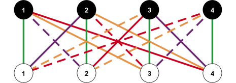
Figure 2: The cis-adinkra (left) and trans-adinkra (right). The graphs are identical aside from the orange transformation laws, which are dashed in one graph and solid in the other. This is reflected in the ${\rm D}_{3}$ transformation laws which differ by a minus sign.

Table 1: The number of cis-adinkras $n_{c}$ and trans-adinkras $n_{t}$ used to decompose various 4D, $\mathcal{N}=1$ multiplets and their associated value of $\chi_{0}=n_{c}-n_{t}$.

Multiplet	CM	VM	TM	CLS	mSG	$\not$mSG	cSG
$n_{c}$	1	0	0	1	1	1	0
$n_{t}$	0	1	1	2	2	4	2
$\chi_{0}$	$+1$	$-1$	$-1$	$-1$	$-1$	$-3$	$-2$

Notice in Table 1 that the values of $n_{c}$ and $n_{t}$ only serve to partially differentiate the various multiplets at the adinkra level. Specifically, the CM is seen to be distinct from the VM and TM, but the VM and TM are indistinguishable based solely on their cis/trans adinkra content. Similarly, there is no difference between CLS and mSG at the adinkra-level. Another tool is needed to completely sort this out.

Dimensional enhancement, or SUSY holography, is the effort to build higher dimensional SUSY representations from lower dimensional representations  [?,?,?]. To aid in sorting out which of the multitude of lower dimensional systems are candidates for dimensional enhancement, a tool known as holoraumy is being developed  [?,?,?,?,?,?,?,?,?,?,?]. On the 0-brane with $N$ SUSY transformations ${\rm D}_{\rm I}$, holoraumy is defined as the commutator of two supersymmetric transformations ${\rm D}_{\rm I}$ acting on the bosons $\Phi$ or fermions $\Psi$ of a particular representation

$$[{\rm D}_{\rm I},{\rm D}_{\rm J}]\Phi= -2i\mathscr{B}_{\rm IJ}\dot{\Phi}$$ (1.1)

$$[{\rm D}_{\rm I},{\rm D}_{\rm J}]\Psi= -2i\mathscr{F}_{\rm IJ}\dot{\Psi}.$$ (1.2)

where a dot above a field indicates a time derivative, $\dot{\Phi}=d\Phi/d\tau$ for example. Contrast holoraumy with the SUSY algebra, which is the anti-commutator of two SUSY transformations ${\rm D}_{\rm I}$. A closed 1D SUSY algebra takes the following form on all fields

$$\{{\rm D}_{\rm I},{\rm D}_{\rm J}\}=2i\delta_{\rm IJ}\partial_{\tau}.$$ (1.3)

Holoraumy is the tool being developed to split the degeneracy of the cis- and trans-information, as shown in Table 1. For instance, holoraumy was first shown to separate the VM and TM at the adinkra level in  [?,?]. To do so, a dot product-like “gadget” was introduced in  [?,?] and studied further in  [?,?,?,?,?].

In this paper, we further the supersymmetry genomics efforts by decomposing the two representations of 4D, $\mathcal{N}=1$ matter gravitino, one as described in  [?,?,?] and the other as described in  [?,?], in terms of the cis- and trans-adinkra content as well as their holoraumy. These multiplets have the same degrees of freedom (20 bosons and 20 fermions) as $\not$mSG  [?], thus we compare their cis- and trans-adinkra and holoraumy to this multiplet as well. To the knowledge of the authors, this paper is the first time that the transformation laws for the two matter gravitino multiplets and $\not$mSG  have each been written in terms of a one-parameter family of transformation laws that encodes a field redefinition of the auxiliary fermions that preserves the diagonal character of the Lagrangian. The parameter is discussed in  [?], but the transformation laws described there are in terms of a specific value of the parameter. Whereas the cis- and trans-adinkra content are shown to be independent of this parameter, the holoraumy is not. Adinkras such as those in Figure 2 can be transformed amongst each other via signed permutations of the colors and/or nodes. For the adinkras in Figure 2, the group to perform these transformation is $BC_{4}$: the group of signed permutations of four elements. Recently, $BC_{4}$ transformations between adinkras of different holoraumy-equivalence classes were worked out in  [?] for adinkras such as those in Figure 2. In a sense, this paper is a sister paper of the recent work  [?]: this paper reviews the status of SUSY genomics, focusing on 4D dynamics, whereas  [?] reviews the status of SUSY holography, focusing on 1D dynamics. It is the view of at least one of the authors of this paper (KS) that building a complete picture of SUSY holography  [?,?,?] would require efforts into SUSY genomics  [?,?,?], enumeration techniques  [?,?], and classification schemes  [?,?,?,?,?,?,?,?,?,?,?]. The main results of the paper are as follows:

1. This paper presents the Majorana representation of the $O(1)$ transformation laws of the multiplet described in  [?,?,?]. The existence of these transformation laws is discussed in  [?,?] as a submultiplet of the overarching $SO(2)$ transformation laws. In  [?], the $O(1)$ submultiplet’s tranformation laws are presented in a Weyl representation. It is important to have a Majorana representation of component transformation laws for a multiplet to be decomposed as adinkras as in the previous genomics works  [?,?,?].

2. The transformation laws for the two matter-gravitino multiplets and $\not$mSG  are expressed in terms of a field redefinition parameter that preserves the diagonal character of the Lagrangian. The existence of this parameter is pointed out in  [?]. As we plan to further SUSY genomics and holography research to higher spin multiplets, where this diagonal parameter continues to be present, it is important to understand this parameter’s significance at the adinkra level.

3. This paper demonstrates the utility of the new Mathematica package Adinkra.m (https://hepthools.github.io/Adinkra/). This package is available open-source and will be indispensable in future adinkra research.

4. The main purpose of the paper is the adinkranization of the two matter-gravitino multiplets, the calculation of their fermionic holoraumy matrices along with that of $\not$mSG, and the comparisons between these three multiplets via the gadget. In calculations of holoraumy and the gadget of these three multiplets, we see the presence of the diagonal Lagrangian parameter. The gadget results presented in this paper will provide a template for researching the significance of this parameter in future, higher spin investigations as pertaining to SUSY genomics and holography. The $20\times 20$ multiplets investigated in this paper are the base of a tower of higher spin multiplets  [?,?,?,?], thus they lay the foundation for future investigations of these higher spin multiplets.

This paper is organized as follows. In Section 2, we review adinkras. In Section 3, we review supersymmetry genomics. Sections 4–6 review the two matter gravitino multiplets and the $\not$mSG multiplet, expressed in terms of the one parameter diagonal Lagrangian family of transformations. Section 7 presents the adinkra and 1D holoraumy content of each of the $20\times 20$ multiplets and makes comparisons via the gadget. For all gamma matrix conventions, we follow precisely the previous three supersymmetry genomics works  [?,?,?].

2 Adinkra Review

Adinkras are graphs that encode supersymmetry transformation laws in one dimension (that of time $\tau$) with complete fidelity. Take for example four dynamical bosonic fields $\Phi_{i}$ and four dynamical fermionic fields $\Psi_{\hat{j}}$ that depend only on time. Two distinct possible sets of supersymmetry transformation laws for $\Phi_{i}$ and $\Psi_{\hat{j}}$ can be succinctly encoded as

$$\text{${\rm D}_{1}$}\Phi_{1}= i\Psi_{1},~{}~{}~{}\text{${\rm D}_{2}$}\Phi_{1}=i\Psi_{2},~{}~{}~{}\text{${\rm D}_{3}$}\Phi_{1}=\chi_{0}i\Psi_{3},~{}~{}~{}\text{${\rm D}_{4}$}\Phi_{1}=-i\Psi_{4}$$ (2.1a)

$$\text{${\rm D}_{1}$}\Phi_{2}= i\Psi_{2},~{}~{}~{}\text{${\rm D}_{2}$}\Phi_{2}=-i\Psi_{1},~{}~{}~{}\text{${\rm D}_{3}$}\Phi_{2}=\chi_{0}i\Psi_{4},~{}~{}~{}\text{${\rm D}_{4}$}\Phi_{2}=i\Psi_{3}$$ (2.1b)

$$\text{${\rm D}_{1}$}\Phi_{3}= i\Psi_{3},~{}~{}~{}\text{${\rm D}_{2}$}\Phi_{3}=-i\Psi_{4},~{}~{}~{}\text{${\rm D}_{3}$}\Phi_{3}=-\chi_{0}i\Psi_{1},~{}~{}~{}\text{${\rm D}_{4}$}\Phi_{3}=-i\Psi_{2}$$ (2.1c)

$$\text{${\rm D}_{1}$}\Phi_{4}= i\Psi_{4},~{}~{}~{}\text{${\rm D}_{2}$}\Phi_{4}=i\Psi_{3},~{}~{}~{}\text{${\rm D}_{3}$}\Phi_{4}=-\chi_{0}i\Psi_{2},~{}~{}~{}\text{${\rm D}_{4}$}\Phi_{4}=i\Psi_{1}$$ (2.1d)

and

$$\text{${\rm D}_{1}$}\Psi_{1}= \dot{\Phi}_{1},~{}~{}~{}\text{${\rm D}_{2}$}\Psi_{1}=-\dot{\Phi}_{2},~{}~{}~{}\text{${\rm D}_{3}$}\Psi_{1}=-\chi_{0}\dot{\Phi}_{3},~{}~{}~{}\text{${\rm D}_{4}$}\Psi_{1}=\dot{\Phi}_{4}$$ (2.2a)

$$\text{${\rm D}_{1}$}\Psi_{2}= \dot{\Phi}_{2},~{}~{}~{}\text{${\rm D}_{2}$}\Psi_{2}=\dot{\Phi}_{1},~{}~{}~{}\text{${\rm D}_{3}$}\Psi_{2}=-\chi_{0}\dot{\Phi}_{4},~{}~{}~{}\text{${\rm D}_{4}$}\Psi_{2}=-\dot{\Phi}_{3}$$ (2.2b)

$$\text{${\rm D}_{1}$}\Psi_{3}= \dot{\Phi}_{3},~{}~{}~{}\text{${\rm D}_{2}$}\Psi_{3}=\dot{\Phi}_{4},~{}~{}~{}\text{${\rm D}_{3}$}\Psi_{3}=\chi_{0}\dot{\Phi}_{1},~{}~{}~{}\text{${\rm D}_{4}$}\Psi_{3}=\dot{\Phi}_{2}$$ (2.2c)

$$\text{${\rm D}_{1}$}\Psi_{4}= \dot{\Phi}_{4},~{}~{}~{}\text{${\rm D}_{2}$}\Psi_{4}=-\dot{\Phi}_{3},~{}~{}~{}\text{${\rm D}_{3}$}\Psi_{4}=\chi_{0}\dot{\Phi}_{2},~{}~{}~{}\text{${\rm D}_{4}$}\Psi_{4}=-\dot{\Phi}_{1}$$ (2.2d)

where a dot above a field indicates a time derivative, $\dot{\Phi}_{i}=d\Phi_{i}/d\tau$ for example. One set of transformation laws is encoded by the choice $\chi_{0}=+1$ and another by $\chi_{0}=-1$. For Equations (2.1) and (2.2), there is no possible set of field redefinitions for which the $\chi_{0}=+1$ transformation laws reduce to the transformation laws for which $\chi_{0}=-1$. Owing to an analogy to isomers in chemistry, in  [?], the $\chi_{0}=+1$ transformation laws were dubbed the cis-multiplet and $\chi_{0}=-1$ the trans-multiplet. Both the cis- and trans-transformation laws satisfy the closure relationship, Equation (1.3).

The adinkras in Figure 2 can be seen to encode the transformation laws in Equations (2.1) and (2.2) as follows.

1. The white nodes encode the bosons $\Phi_{i}$ and the black nodes encode the fermions multiplied by the imaginary number $i\Psi_{\hat{j}}$.

2. A line connecting two nodes indicates a SUSY transformation law between the corresponding fields.

3. Each of the $N=4$ colors encodes a different SUSY transformation as color coded in Equations (2.1) and (2.2).

4. A solid (dashed) line indicates a plus (minus) sign in SUSY transformations.

5. In transforming from a higher node to a lower node (higher mass dimension field to one-half lower mass dimension field), a time derivative appears on the field of the lower node.

The adinkras in Figure 2 are known as valise adinkras: adinkras with a single row of bosons and a single row of fermions. The distinction between the two set of transformation laws encoded in Equations (2.1) and (2.2) can be seen easily in the adinkras in Figure 2: the two adinkras are identical aside from the orange lines, which are dashed in one adinkra and solid in the other. This is reflected in the ${\rm D}_{3}$ transformation laws in Equations (2.1) and (2.2), which differ by a minus sign.

Both $\chi_{0}=\pm 1$ supersymmetric transformation laws are symmetries of the Lagrangian

$$\mathcal{L}=\frac{1}{2}\delta^{ij}\dot{\Phi}_{i}\dot{\Phi}_{j}-i\frac{1}{2}\delta^{\hat{i}\hat{j}}\Psi_{\hat{i}}\dot{\Psi}_{\hat{j}}.$$ (2.3)

The transformation laws in Equations (2.1) and (2.2) can succinctly be written as

$${\rm D}_{\rm I}\Phi=i{{\boldsymbol{\rm L}}}_{\rm I}\Psi,~{}~{}~{}{\rm D}_{\rm I}\Psi={{\boldsymbol{\rm R}}}_{\rm I}\dot{\Phi},$$ (2.4)

where the adinkra matrices ${{\boldsymbol{\rm L}}}_{\rm I}$ are given by

$${{\boldsymbol{\rm L}}}_{1}=\left(\begin{array}[]{cccc}1&0&0&0\\ 0&1&0&0\\ 0&0&1&0\\ 0&0&0&1\\ \end{array}\right) ,~{}~{}~{}\mbox{ { ${{\boldsymbol{\rm L}}}_{2}=\left(\begin{array}[]{cccc}0&1&0&0\\ -1&0&0&0\\ 0&0&0&-1\\ 0&0&1&0\\ \end{array}\right)\ $}},$$ (2.13)

$${{\boldsymbol{\rm L}}}_{3}=\chi_{0}\left(\begin{array}[]{cccc}0&0&1&0\\ 0&0&0&1\\ -1&0&0&0\\ 0&-1&0&0\\ \end{array}\right) ,~{}~{}~{}\mbox{ { ${{\boldsymbol{\rm L}}}_{4}=\left(\begin{array}[]{cccc}0&0&0&-1\\ 0&0&1&0\\ 0&-1&0&0\\ 1&0&0&0\\ \end{array}\right)$}}$$ (2.22)

and the ${{\boldsymbol{\rm R}}}_{\rm I}$ given by

$${{\boldsymbol{\rm R}}}_{\rm I}={{\boldsymbol{\rm L}}}_{\rm I}^{-1}.$$ (2.23)

In the specific case of the matrices in Equation (2.13), we also have the orthogonality relationship

$${{\boldsymbol{\rm R}}}_{\rm I}={{\boldsymbol{\rm L}}}_{\rm I}^{-1}={{\boldsymbol{\rm L}}}_{\rm I}^{T}~{}~{}~{}$$ (2.24)

where the $T$ denotes transpose. Supersymmetric multiplets whose adinkra matrices satisfy the orthogonality relationship (Equation (2.24)) are said to be adinkraic representations, that is, they can be expressed as adinkras pictures as in Figures 1 and 2. Generally, larger multiplets such as those investigated in this paper are non-adinkraic when nodes are chosen to be identified with single fields as reviewed in Sections 3.4 and 3.5. Non-adinkraic multiplets have been investigated previously in  [?,?].

The closure relation, Equation (1.3), for an adinkriac system is reflected in the adinkra matrices ${{\boldsymbol{\rm L}}}_{\rm I}$ and ${{\boldsymbol{\rm R}}}_{\rm I}$ satisfying the $\mathcal{GR}(d,N)$ algebra also known as the garden algebra  [?,?]

$${{\boldsymbol{\rm L}}}_{\rm I}{{\boldsymbol{\rm R}}}_{\rm J}+{{\boldsymbol{\rm L}}}_{\rm J}{{\boldsymbol{\rm R}}}_{\rm I}=2\delta_{\rm IJ}{{\boldsymbol{\rm I}}}_{4},~{}~{}~{}{{\boldsymbol{\rm R}}}_{\rm I}{{\boldsymbol{\rm L}}}_{\rm J}+{{\boldsymbol{\rm R}}}_{\rm J}{{\boldsymbol{\rm L}}}_{\rm I}=2\delta_{\rm IJ}{{\boldsymbol{\rm I}}}_{4}.$$ (2.25)

The $\mathcal{GR}(d,N)$ algebra is the algebra of general, real matrices encoding the supersymmetry transformation laws between $d$ bosons, $d$ fermions, and $N$ supersymmetries. Specifically, all the $\chi_{0}=\pm 1$ adinkras in Figure 2 satisfy the $\mathcal{GR}(4,4)$ algebra.

For an arbitrary $d$, $N=4$ adinkra, $\chi_{0}$ can be defined off the following chromocharacter equation  [?]

$$Tr({{\boldsymbol{\rm L}}}_{\rm I}{{\boldsymbol{\rm R}}}_{\rm J}{{\boldsymbol{\rm L}}}_{\rm K}{{\boldsymbol{\rm R}}}_{\rm L})=4[(n_{c}+n_{t})(\delta_{{\rm I}{\rm J}}\delta_{{\rm K}{\rm L}}-\delta_{{\rm I}{\rm L}}\delta_{{\rm J}{\rm K}}+\delta_{{\rm I}{\rm J}}\delta_{{\rm K}{\rm L}})+\chi_{0}~{}\epsilon_{{\rm I}{\rm J}{\rm K}{\rm L}}]~{}~{}~{}$$ (2.26)

Calculating $\chi_{0}$ through Equation (2.26) allows one to immediately determine $n_{c}$ and $n_{t}$ which satisfy  [?,?,?]

$$n_{c}=\frac{d}{8}+\frac{\chi_{0}}{2}$$ (2.27)

$$n_{t}=\frac{d}{8}-\frac{\chi_{0}}{2}$$ (2.28)

For $\mathcal{GR}(4,4)$ valise adinkras, the only two possible values are $\chi_{0}=\pm 1$  [?] and either $n_{c}=1,~{}n_{t}=0$ or $n_{c}=0,~{}n_{t}=1$.

The matrix representation of 1D holoraumy, Equation (1.1), is  [?,?]

$${{\boldsymbol{\rm V}}}_{{\rm I}{\rm J}}= -\frac{i}{2}\textbf{L}_{[I}\textbf{R}_{J]},~{}~{}~{}{{\boldsymbol{\widetilde{\rm V}}}}_{{\rm I}{\rm J}}=-\frac{i}{2}\textbf{R}_{[I}\textbf{L}_{J]}.$$ (2.29)

where ${{\boldsymbol{\rm V}}}_{{\rm I}{\rm J}}$ is the matrix representation of the bosonic holoraumy tensor $\mathscr{B}_{\rm IJ}$ and ${{\boldsymbol{\widetilde{\rm V}}}}_{\rm IJ}$ is the matrix representation of the fermionic holoraumy tensor $\mathscr{F}_{\rm IJ}$. Adinkras that share the same value of $\chi_{0}$ and have the same number of degrees of freedom $d$ are said to be in the same $\chi_{0}$-equivalence class  [?]. There are two possible $\chi_{0}$-equivalence classes for $\mathcal{GR}(4,4)$ valise adinkras: the cis-equivalence class defined by $\chi_{0}=+1$ and the trans-equivalence class defined by $\chi_{0}=-1$. In  [?], all possible 36,864 $\mathcal{GR}(4,4)$ adinkras were investigated and tabulated and in  [?] all were categorized in terms of $\chi_{0}$-equivalence classes and holoraumy-equivalence classes.

3 Supersymmetry Genomics Review

In this section, we review the previous SUSY genomics works  [?,?,?]. In doing so, we demonstrate how the the cis-adinkra and trans-adinkra shown in Figure 2 encode the 0-brane reduced transformation laws for various 4D, $\mathcal{N}=1$ off-shell multiplets and comment on their values of $\chi_{0}$, holoraumy, and gadgets in the cases where this is known.

3.1 The 4D, $\mathcal{N}=1$ Off-Shell Chiral Multiplet (CM)

The dynamical field content of the CM is a scalar $A$, pseudoscalar $B$, and Majorana fermion $\psi_{a}$. The auxiliary field content of the CM is a scalar $F$ and pseudoscalar $G$. The 4D component Lagrangian for the CM is given by

 

$${{\mathcal{L}}_{\text{CM}}=}$$

  (3.1)

The transformation laws that are a symmetry of the Lagrangian in Equation (3.1) are

 

$${{\rm D}_{a}A~{}}$$

  (3.2)

Reducing to the 0-brane with nodal field definitions

$$i\Psi_{1}=\psi_{1},~{}~{}~{}i\Psi_{2}=\psi_{2},~{}~{}~{}i\Psi_{3}=\psi_{3},~{}~{}~{}i\Psi_{4}=\psi_{4}~{}~{}~{}$$ (3.3a)

$$\Phi_{1}=A,~{}~{}~{}\Phi_{2}=B,~{}~{}~{}\Phi_{3}=\int d\tau~{}F,~{}~{}~{}\Phi_{4}=\int d\tau~{}G~{}~{}~{}$$ (3.3b)

reduces the Lagrangian in Equation (3.1) to Equation (2.3) and transformation laws to Equation (2.4) with the ${{\boldsymbol{\rm L}}}_{\rm I}$ matrices given by

$${{\boldsymbol{\rm L}}}^{(\text{CM})}_{1}=\left(\begin{array}[]{cccc}1&0&0&0\\ 0&0&0&-1\\ 0&1&0&0\\ 0&0&-1&0\\ \end{array}\right) ,~{}~{}~{}\mbox{ { ${{\boldsymbol{\rm L}}}_{2}^{(\text{CM})}=\left(\begin{array}[]{cccc}0&1&0&0\\ 0&0&1&0\\ -1&0&0&0\\ 0&0&0&-1\\ \end{array}\right)$}},$$ (3.12)

$${{\boldsymbol{\rm L}}}_{3}^{(\text{CM})}=\left(\begin{array}[]{cccc}0&0&1&0\\ 0&-1&0&0\\ 0&0&0&-1\\ 1&0&0&0\\ \end{array}\right) ,~{}~{}~{}\mbox{ { ${{\boldsymbol{\rm L}}}_{4}^{(\text{CM})}=\left(\begin{array}[]{cccc}0&0&0&1\\ 1&0&0&0\\ 0&0&1&0\\ 0&1&0&0\\ \end{array}\right)$}}.$$ (3.21)

and ${{\boldsymbol{\rm R}}}_{\rm I}$ given by Equation (2.24) and satisfy the $\mathcal{GR}(4,4)$ algebra Equation (2.25). By the rules explained in Section 2, it can be seen that the 0-brane transformation laws for the CM, Equation (2.4), with ${{\boldsymbol{\rm L}}}_{\rm I}$ and ${{\boldsymbol{\rm R}}}_{\rm I}$ matrices as in Equations (3.12) and (2.24) and nodal field definitions (Equation (3.3)), are entirely described by the adinkra in Figure 3, which is the same image as Figure 1 in the Introduction. The CM is in the cis-equivalence class as can be seen in the following two ways

1. Calculating the trace in Equation (2.26), which produces the result $\chi_{0}=+1$.

2. Performing certain field redefinitions, as in  [?], that transform Figure 3 into the cis-adinkra in Figure 2.

The field redefinitions mentioned in the second of these are dubbed flips and flops in the recent work  [?].

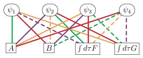
Figure 3: This is identical to Figure 1: An adinkra for the 0-brane reduced transformation laws of the 4D, $\mathcal{N}=1$ chiral multiplet.

3.2 The 4D, $\mathcal{N}=1$ Off-Shell Tensor Multiplet (TM)

The dynamical field content of the TM is a scalar $\varphi$, anti-symmetric rank-two tensor $B_{\mu\nu}$, and a Majorana fermion $\chi_{a}$. There are no auxiliary fields in the TM. The 4D component Lagrangian for the TM is given by

 

$${\mathcal{L}_{\text{TM}}=}$$

  (3.22)

where

$$H_{\mu\nu\alpha}\equiv\partial_{\mu}B_{\nu\alpha}+\partial_{\nu}B_{\alpha\mu}+\partial_{\alpha}B_{\mu\nu}$$ (3.23)

The transformation laws that are a symmetry of the Lagrangian in Equation (3.22) are

 

$${{\rm D}_{a}\varphi~{}}$$

  (3.24)

Choosing temporal gauge $B_{0\mu}=0$ and reducing to the 0-brane with nodal field definitions

$$i\Psi_{1}=\chi_{1},~{}~{}~{}i\Psi_{2}=\chi_{2},~{}~{}~{}i\Psi_{3}=\chi_{3},~{}~{}~{}i\Psi_{4}=\chi_{4}~{}~{}~{}$$ (3.25a)

$$\Phi_{1}=\varphi,~{}~{}~{}\Phi_{2}=2B_{12},~{}~{}~{}\Phi_{3}=2B_{23},~{}~{}~{}\Phi_{4}=2B_{31}~{}~{}~{}$$ (3.25b)

reduces the Lagrangian in Equation (3.22) to Equation (2.3) and transformation laws to Equation (2.4) with the ${{\boldsymbol{\rm L}}}_{\rm I}$ matrices given by

$${{\boldsymbol{\rm L}}}_{1}^{(\text{TM})}=\left(\begin{array}[]{cccc}1&0&0&0\\ 0&0&-1&0\\ 0&0&0&-1\\ 0&-1&0&0\\ \end{array}\right) ,~{}~{}~{}\mbox{ { ${{\boldsymbol{\rm L}}}_{2}^{(\text{TM})}=\left(\begin{array}[]{cccc}0&1&0&0\\ 0&0&0&1\\ 0&0&-1&0\\ 1&0&0&0\\ \end{array}\right)$}},$$ (3.34)

$${{\boldsymbol{\rm L}}}_{3}^{(\text{TM})}=\left(\begin{array}[]{cccc}0&0&1&0\\ 1&0&0&0\\ 0&1&0&0\\ 0&0&0&-1\\ \end{array}\right) ,~{}~{}~{}\mbox{ { ${{\boldsymbol{\rm L}}}_{4}^{(\text{TM})}=\left(\begin{array}[]{cccc}0&0&0&1\\ 0&-1&0&0\\ 1&0&0&0\\ 0&0&1&0\\ \end{array}\right)$}}$$ (3.43)

and ${{\boldsymbol{\rm R}}}_{\rm I}$ given by Equation (2.24) and satisfy the $\mathcal{GR}(4,4)$ algebra in Equation (2.25). By the rules explained in Section 2, it can be seen that the 0-brane transformation laws for the TM, Equation (2.4) with ${{\boldsymbol{\rm L}}}_{\rm I}$ and ${{\boldsymbol{\rm R}}}_{\rm I}$ matrices as in Equations (3.34) and (2.24) and nodal field definitions (Equation (3.25)), are described by the adinkra in Figure 4. The TM is in the trans-equivalence class ($\chi_{0}=-1$) as can be seen through either Equation (2.26) or through field redefinitions transforming Figure 4 into the trans-adinkra in Figure 2.

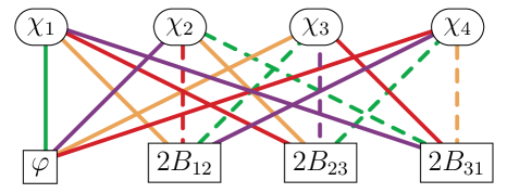
Figure 4: An adinkra for the 0-brane reduced transformation laws of the 4D, $\mathcal{N}=1$ tensor multiplet.

3.3 The 4D, $\mathcal{N}=1$ Off-Shell Vector Multiplet (VM)

The dynamical field content of the VM is a $U(1)$ gauge vector field $A_{\mu}$ and a Majorana fermion $\lambda_{a}$. The only auxiliary field in the VM is a pseudoscalar ${\rm d}$. The 4D component Lagrangian for the VM is given by

 

$${{\mathcal{L}}_{\text{VM}}=}$$

  (3.44)

where

$$F_{\mu\nu}=\partial_{\mu}A_{\nu}-\partial_{\nu}A_{\mu}$$ (3.45)

The transformation laws that are a symmetry of the Lagrangian in Equation (3.44) are

 

$${{\rm D}{}_{a}A_{\mu}}$$

  (3.46)

Choosing temporal gauge $A_{0}=0$ and reducing to the 0-brane with nodal field definitions

$$i\Psi_{1}=\lambda_{1},~{}~{}~{}i\Psi_{2}=\lambda_{2},~{}~{}~{}i\Psi_{3}=\lambda_{3},~{}~{}~{}i\Psi_{4}=\lambda_{4}~{}~{}~{}$$ (3.47a)

$$\Phi_{1}=A_{1},~{}~{}~{}\Phi_{2}=A_{2},~{}~{}~{}\Phi_{3}=A_{3},~{}~{}~{}\Phi_{4}=\int d\tau~{}{\rm d}~{}~{}~{}$$ (3.47b)

reduces the Lagrangian in Equation (3.44) to Equation (2.3) and transformation laws to Equation (2.4) with the ${{\boldsymbol{\rm L}}}_{\rm I}$ matrices given by

$${{\boldsymbol{\rm L}}}_{1}^{(\text{VM})}=\left(\begin{array}[]{cccc}0&1&0&0\\ 0&0&0&-1\\ 1&0&0&0\\ 0&0&-1&0\\ \end{array}\right) ,~{}~{}~{}\mbox{ { ${{\boldsymbol{\rm L}}}_{2}^{(\text{VM})}=\left(\begin{array}[]{cccc}1&0&0&0\\ 0&0&1&0\\ 0&-1&0&0\\ 0&0&0&-1\\ \end{array}\right)$}},$$ (3.56)

$${{\boldsymbol{\rm L}}}_{3}^{(\text{VM})}=\left(\begin{array}[]{cccc}0&0&0&1\\ 0&1&0&0\\ 0&0&1&0\\ 1&0&0&0\\ \end{array}\right) ,~{}~{}~{}\mbox{ { ${{\boldsymbol{\rm L}}}_{4}^{(\text{VM})}=\left(\begin{array}[]{cccc}0&0&1&0\\ -1&0&0&0\\ 0&0&0&-1\\ 0&1&0&0\\ \end{array}\right)$}}$$ (3.65)

and ${{\boldsymbol{\rm R}}}_{\rm I}$ given by Equation (2.24) and satisfy the $\mathcal{GR}(4,4)$ algebra in Equation (2.25). By the rules explained in Section 2, it can be seen that the 0-brane transformation laws for the VM, Equation (2.4), with ${{\boldsymbol{\rm L}}}_{\rm I}$ and ${{\boldsymbol{\rm R}}}_{\rm I}$ matrices as in Equations (3.56) and (2.24) and nodal field definitions (Equation (3.47)), are described the adinkra in Figure 5. The VM is in the trans-equivalence class ($\chi_{0}=-1$) as can be seen through either Equation (2.26) or through field redefinitions transforming Figure 5 into the trans-adinkra in Figure 2.

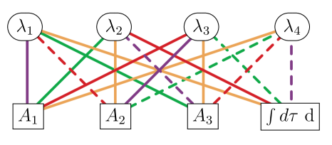
Figure 5: An adinkra for the 0-brane reduced transformation laws of the 4D, $\mathcal{N}=1$ vector multiplet.

3.4 The 4D, $\mathcal{N}=1$ Off-Shell Complex Linear Superfield Multiplet (CLS)

The dynamical field content of the CLS is the same as for the CM: a scalar field and pseudoscalar field, here called $K$ and $L$, respectively, and a Majorana fermion, here called $\zeta_{a}$. A key difference from CLS and CM is the auxiliary field content: a scalar $M$, pseudoscalar $N$, vector $V_{\mu}$, pseudovector $U_{\mu}$, a low-dimensional fermion $\rho_{a}$ with $[\rho_{a}]=3/2$ and a high-dimensional fermion $\beta_{a}$ with $[\beta_{a}]=5/2$. The 4D component Lagrangian for CLS is

 

$${\mathcal{L}_{\text{CLS}}}$$

  (3.66)

The transformation laws that are a symmetry of the Lagrangian in Equation (3.66) are

$$\begin{split}{\rm D}_{a}K=&\rho_{a}-\zeta_{a}\cr{\rm D}_{a}M=&\beta_{a}-\frac{1}{2}(\gamma^{\nu})_{a}^{\,\,\,d}\partial_{\nu}\rho_{d}\cr{\rm D}_{a}N=&-i(\gamma^{5})_{a}^{\,\,\,\,d}\beta_{d}+\frac{i}{2}(\gamma^{5}\gamma^{\nu})_{a}^{\,\,\,d}\partial_{\nu}\rho_{d}\cr{\rm D}_{a}L=&i(\gamma^{5})_{a}^{\,\,\,d}(\rho_{d}+\zeta_{d})\cr{\rm D}_{a}U_{\mu}=&i(\gamma^{5}\gamma_{\mu})_{a}^{\,\,\,\,d}\beta_{d}-i(\gamma^{5})_{a}^{\,\,\,\,d}\partial_{\mu}(\rho_{d}+2\zeta_{d})-\frac{i}{2}\,(\gamma^{5}\gamma^{\nu}\gamma_{\mu})_{a}^{\,\,\,d}\partial_{\nu}(\rho_{d}-2\zeta_{d})\cr{\rm D}_{a}V_{\mu}=&-(\gamma_{\mu})_{a}^{\,\,\,\,d}\beta_{d}+\partial_{\mu}(\rho_{a}-2\zeta_{a})+\frac{1}{2}(\gamma^{\nu}\gamma_{\mu})_{a}^{\,\,\,d}\partial_{\nu}(\rho_{d}+2\zeta_{d})\cr{\rm D}_{a}\zeta_{b}=&-i(\gamma^{\mu})_{ab}\partial_{\mu}K-(\gamma^{5}\gamma^{\mu})_{ab}\partial_{\mu}L-\,\frac{1}{2}(\gamma^{5}\gamma^{\mu})_{ab}U_{\mu}+i\frac{1}{2}(\gamma^{\mu})_{ab}V_{\mu}\cr{\rm D}_{a}\rho_{b}=&iC_{ab}M+(\gamma^{5})_{ab}N+\,\frac{1}{2}(\gamma^{5}\gamma^{\mu})_{ab}U_{\mu}+i\frac{1}{2}(\gamma^{\mu})_{ab}V_{\mu}\cr{\rm D}_{a}\beta_{b}=&\frac{i}{2}(\gamma^{\mu})_{ab}\partial_{\mu}M+\frac{1}{2}(\gamma^{5}\gamma^{\mu})_{ab}\partial_{\mu}N+\frac{1}{2}(\gamma^{5}\gamma^{\mu}\gamma^{\nu})_{ab}\partial_{\mu}U_{\nu}\cr&+\frac{1}{4}(\gamma^{5}\gamma^{\nu}\gamma^{\mu})_{ab}\partial_{\mu}U_{\nu}+\frac{i}{2}(\gamma^{\mu}\gamma^{\nu})_{ab}\partial_{\mu}V_{\nu}+\frac{i}{4}\,(\gamma^{\nu}\gamma^{\mu})_{ab}\partial_{\mu}V_{\nu}\cr&+\eta^{\mu\nu}\partial_{\mu}\partial_{\nu}(-iC_{ab}K+(\gamma^{5})_{ab}L).\end{split}$$ (3.67)

Unlike the minimal CM, TM, and VM cases, the 0-brane reduction for CLS requires nodal definitions that are linear combinations of the 0-brane reduced fields for the resulting ${{\boldsymbol{\rm L}}}_{\rm I}$ matrices to be adinkraic (Equation (2.24)). A particular choice of nodal field definitions for CLS that are adinkraic are

$$\dot{\Phi}=\left(\begin{array}[]{c}-M\\ \dot{K}-V_{0}\\ -\dot{L}-U_{0}\\ N\\ U_{2}\\ V_{0}-2\dot{K}\\ -U_{1}\\ U_{3}\\ -V_{3}\\ V_{1}\\ -2\dot{L}-U_{0}\\ V_{2}\end{array}\right),~{}~{}~{}i\dot{\Psi}=\left(\begin{array}[]{c}\frac{\dot{\rho}_{2}}{2}-\beta_{1}\\ -\beta_{2}-\frac{\dot{\rho}_{1}}{2}\\ -\beta_{3}-\frac{\dot{\rho}_{4}}{2}\\ \beta_{4}-\frac{\dot{\rho}_{3}}{2}\\ \beta_{1}-\dot{\zeta}_{2}+\frac{\dot{\rho}_{2}}{2}\\ \beta_{2}+\dot{\zeta}_{1}-\frac{\dot{\rho}_{1}}{2}\\ \beta_{3}+\dot{\zeta}_{4}-\frac{\dot{\rho}_{4}}{2}\\ \beta_{4}-\dot{\zeta}_{3}+\frac{\dot{\rho}_{3}}{2}\\ \beta_{1}+\dot{\zeta}_{2}+\frac{\dot{\rho}_{2}}{2}\\ -\beta_{2}+\dot{\zeta}_{1}+\frac{\dot{\rho}_{1}}{2}\\ -\beta_{3}+\dot{\zeta}_{4}+\frac{\dot{\rho}_{4}}{2}\\ \beta_{4}+\dot{\zeta}_{3}+\frac{\dot{\rho}_{3}}{2}\end{array}\right)$$ (3.68)

Here, we define $\Phi$ and $\Psi$ in terms of their derivatives $\dot{\Phi}$ and $\dot{\Psi}$ for notational convenience (integration constants are assumed to be zero). With these nodal field definitions, the Lagrangian in Equation (3.66) reduces to Equation (2.3) and transformation laws to Equation (2.4) with the ${{\boldsymbol{\rm L}}}_{\rm I}$ matrices given by

$$\begin{split}\mbox{{ ${{\boldsymbol{\rm L}}}_{1}^{(\text{CLS})}={{\boldsymbol{\rm I}}}_{3}\otimes{{\boldsymbol{\rm I}}}_{4}$}},~{}~{}~{}&\mbox{{ ${{\boldsymbol{\rm L}}}_{2}^{(\text{CLS})}=i{{\boldsymbol{\rm I}}}_{3}\otimes{{\boldsymbol{\beta}}}_{3}$}}\\ \mbox{{ ${{\boldsymbol{\rm L}}}_{3}^{(\text{CLS})}=i\left(\begin{array}[]{ccc}1&0&0\\ 0&-1&0\\ 0&0&-1\end{array}\right)\otimes{{\boldsymbol{\beta}}}_{2}$}},~{}~{}~{}&\mbox{{ ${{\boldsymbol{\rm L}}}_{4}^{(\text{CLS})}=-i{{\boldsymbol{\rm I}}}_{3}\otimes{{\boldsymbol{\beta}}}_{1}$}}\end{split}$$ (3.69)

with the ${{\boldsymbol{\alpha}}}$ and ${{\boldsymbol{\beta}}}$ matrices as in Appendix C and ${{\boldsymbol{\rm R}}}_{\rm I}$ given by Equation (2.24).

By the rules explained in Section 2, it can be seen that the 0-brane transformation laws for the CLS, Equation (2.4) with ${{\boldsymbol{\rm L}}}_{\rm I}$ matrices as in Equation (3.69) and nodal field definitions (Equation (3.68)), are described by the adinkra in Figure 6. The CLS has $\chi_{0}=-1$ as can be seen through either Equation (2.26) or through the fact that comparing Figure 6 with Figure 2, Figure 6 is one cis-adinkra ($n_{c}=1$) and two trans-adinkras ($n_{t}=2$), thus $\chi_{0}=n_{c}-n_{t}=-1$.

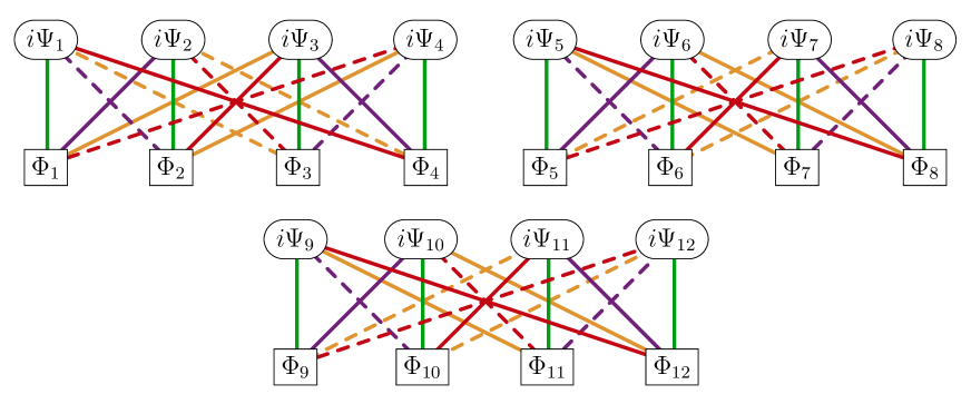
Figure 6: An adinkra for the 0-brane reduced transformation laws of the 4D, $\mathcal{N}=1$ complex linear superfield multiplet (CLS) and old-minimal supergravity multiplet (mSG).

3.5 The 4D, $\mathcal{N}=1$ Off-Shell Old-Minimal Supergravity Multiplet (mSG)

The dynamical field content of mSG is the symmetric, rank two graviton $h_{\mu\nu}$ and gravitino $\psi_{\mu a}$. The auxiliary fields of mSG are a scalar $S$, pseudoscalar $P$, and axial vector $A_{\mu}$. The 4D component Lagrangian for mSG is

$$\mathcal{L}_{mSG}= -\frac{1}{2}\partial_{\alpha}h_{\mu\nu}\partial^{\alpha}h^{\mu\nu}+\frac{1}{2}\partial^{\alpha}h\partial_{\alpha}h-\partial^{\alpha}h\partial^{\beta}h_{\alpha\beta}+\partial^{\mu}h_{\mu\nu}\partial_{\alpha}h^{\alpha\nu}$$ (3.70)

$$-\frac{1}{3}S^{2}-\frac{1}{3}P^{2}+\frac{1}{3}A_{\mu}A^{\mu}-\frac{1}{2}\psi_{\mu a}\epsilon^{\mu\nu\alpha\beta}(\gamma^{5}\gamma_{\nu})^{ab}\partial_{\alpha}\psi_{\beta b}$$ (3.71)

The transformation laws that are a symmetry of the Lagrangian in Equation (3.70) are

$${\rm D}_{a}S=~{} -\frac{1}{2}([\gamma^{\mu},\gamma^{\nu}])_{a}^{~{}b}\partial_{\mu}\psi_{\nu b}$$ (3.72a)

$${\rm D}_{a}P=~{} \frac{1}{2}(\gamma^{5}[\gamma^{\mu},\gamma^{\nu}])_{a}^{~{}b}\partial_{\mu}\psi_{\nu b}$$ (3.72b)

$${\rm D}_{a}A_{\mu}=~{} i(\gamma^{5}\gamma^{\nu})_{a}^{~{}b}\partial_{[\nu}\psi_{\mu]b}-\frac{1}{2}\epsilon_{\mu}^{~{}\nu\alpha\beta}(\gamma_{\nu})_{a}^{~{}b}\partial_{\alpha}\psi_{\beta b}$$ (3.72c)

$${\rm D}_{a}h_{\mu\nu}=~{} \frac{1}{2}(\gamma_{(\mu})_{a}^{~{}b}\psi_{\nu)b}$$ (3.72d)

$${\rm D}_{a}\psi_{\mu b}=~{} -\frac{i}{3}(\gamma_{\mu})_{ab}S-\frac{1}{3}(\gamma^{5}\gamma_{\mu})_{ab}P+\frac{2}{3}(\gamma^{5})_{ab}A_{\mu}+\frac{1}{6}(\gamma^{5}[\gamma_{\mu},\gamma^{\nu}])_{ab}A_{\nu}+$$ (3.72e)

$$-\frac{i}{2}([\gamma^{\alpha},\gamma^{\beta}])_{ab}\partial_{\alpha}h_{\beta\mu}$$ (3.72f)

Similar to the CLS, the 0-brane reduction for mSG requires nodal definitions that are linear combinations of the 0-brane reduced fields for the resulting ${{\boldsymbol{\rm L}}}_{\rm I}$ matrices to be adinkraic (Equation (2.24)). As shown in  [?], the most general choice of nodal field definitions for mSG that are adinkraic and match with the cis- and/or trans-adinkra Figure 2 are

$$\Phi=\left(\begin{array}[]{c}A_{0}\\ P\\ -S\\ \dot{h}\\ \hline\cr\vspace{-7 pt}\hfil\\ u_{1}A_{1}+(u_{2}-u_{3})\dot{h}_{23}\\ u_{3}A_{3}+(u_{1}-u_{2})\dot{h}_{12}\\ u_{2}A_{2}+(u_{3}-u_{1})\dot{h}_{31}\\ -u_{1}\dot{h}_{11}-u_{2}\dot{h}_{22}-u_{3}\dot{h}_{33}\\ \hline\cr\vspace{-7 pt}\hfil\\ v_{1}A_{1}+(v_{2}-v_{3})\dot{h}_{23}\\ v_{3}A_{3}+(v_{1}-v_{2})\dot{h}_{12}\\ v_{2}A_{2}+(v_{3}-v_{1})\dot{h}_{31}\\ -v_{1}\dot{h}_{11}-v_{2}\dot{h}_{22}-v_{3}\dot{h}_{33}\end{array}\right),~{}~{}~{}i\Psi=\left(\begin{array}[]{c}\dot{\psi}_{13}-\dot{\psi}_{21}-\dot{\psi}_{34}\\ -\dot{\psi}_{14}-\dot{\psi}_{22}-\dot{\psi}_{33}\\ \dot{\psi}_{11}+\dot{\psi}_{23}-\dot{\psi}_{32}\\ \dot{\psi}_{12}-\dot{\psi}_{24}+\dot{\psi}_{31}\\ \hline\cr\vspace{-7 pt}\hfil\\ -u_{1}\dot{\psi}_{13}+u_{2}\dot{\psi}_{21}+u_{3}\dot{\psi}_{34}\\ -u_{1}\dot{\psi}_{14}-u_{2}\dot{\psi}_{22}-u_{3}\dot{\psi}_{33}\\ -u_{1}\dot{\psi}_{11}-u_{2}\dot{\psi}_{23}+u_{3}\dot{\psi}_{32}\\ -u_{1}\dot{\psi}_{12}+u_{2}\dot{\psi}_{24}-u_{3}\dot{\psi}_{31}\\ \hline\cr\vspace{-7 pt}\hfil\\ -v_{1}\dot{\psi}_{13}+v_{2}\dot{\psi}_{21}+v_{3}\dot{\psi}_{34}\\ -v_{1}\dot{\psi}_{14}-v_{2}\dot{\psi}_{22}-v_{3}\dot{\psi}_{33}\\ -v_{1}\dot{\psi}_{11}-v_{2}\dot{\psi}_{23}+v_{3}\dot{\psi}_{32}\\ -v_{1}\dot{\psi}_{12}+v_{2}\dot{\psi}_{24}-v_{3}\dot{\psi}_{31}\end{array}\right)$$ (3.73)

with

$$u_{1}+u_{2}+u_{3}=v_{1}+v_{2}+v_{3}=0$$ (3.74)

Here, we define $\Phi$ and $\Psi$ in terms of their derivatives $\dot{\Phi}$ and $\dot{\Psi}$ for notational convenience as in the CLS case (integration constants are assumed to be zero). With these nodal field definitions, the Lagrangian in Equation (3.70) reduces to Equation (2.3) and transformation laws to Equation (2.4) with the ${{\boldsymbol{\rm L}}}_{\rm I}$ matrices given by

$$\begin{split}\mbox{{ ${{\boldsymbol{\rm L}}}_{1}^{(\text{mSG})}={{\boldsymbol{\rm I}}}_{3}\otimes{{\boldsymbol{\rm I}}}_{4}$}},~{}~{}~{}&\mbox{{ ${{\boldsymbol{\rm L}}}_{2}^{(\text{mSG})}=i{{\boldsymbol{\rm I}}}_{3}\otimes{{\boldsymbol{\beta}}}_{3}$}}\\ \mbox{{ ${{\boldsymbol{\rm L}}}_{3}^{(\text{mSG})}=i\left(\begin{array}[]{ccc}1&0&0\\ 0&-1&0\\ 0&0&-1\end{array}\right)\otimes{{\boldsymbol{\beta}}}_{2}$}},~{}~{}~{}&\mbox{{ ${{\boldsymbol{\rm L}}}_{4}^{(\text{mSG})}=-i{{\boldsymbol{\rm I}}}_{3}\otimes{{\boldsymbol{\beta}}}_{1}$}}\end{split}$$ (3.75)

with the ${{\boldsymbol{\alpha}}}$ and ${{\boldsymbol{\beta}}}$ matrices as in Appendix C and ${{\boldsymbol{\rm R}}}_{\rm I}$ given by Equation (2.24).

By the rules explained in Section 2, it can be seen that the 0-brane transformation laws for the mSG, Equation (2.4) with ${{\boldsymbol{\rm L}}}_{\rm I}$ matrices as in Equation (3.75) and nodal field definitions (Equation (3.73)), are described by the adinkra in Figure 6: the same adinkra as for CLS. Thus, as in the CLS case, the mSG has $\chi_{0}=-1$ and can be decomposed as one cis-adinkra ($n_{c}=1$) and two trans-adinkras ($n_{t}=2$) with $\chi_{0}=n_{c}-n_{t}=-1$.

3.6 Gadgets

There is not a tremendous amount of diversity in the $\chi_{0}$ values reviewed thus far, as summarized in Table 1: all those reviewed in the previous five sections have $\chi_{0}=-1$ aside from the CM, which has $\chi_{0}=+1$. Clearly, another tool is needed to further separate out at the adinkra level which adinkras relate to which higher dimensional systems.

The gadget $\mathcal{G}(\mathcal{R},\mathcal{R}^{\prime})$ between two different adinkra representations $\mathcal{R}$ and $\mathcal{R}^{\prime}$ of the $GR({\rm d},N)$ algebra, defined below, is used to separate multiplets at the adinkra level that holographically correspond to different multiplets in higher dimensions  [?,?,?,?,?,?].

$$\mathcal{G}(\mathcal{R},\mathcal{R}^{\prime})~{} =~{}\frac{(N-2)!}{4(N!)}\sum_{I,J}{{\boldsymbol{\widetilde{\rm V}}}}_{\rm IJ}^{(\mathcal{R})}{{\boldsymbol{\widetilde{\rm V}}}}_{\rm IJ}^{(\mathcal{R}^{\prime})}~{}=~{}\frac{(N-2)!}{{\rm d}_{min}(4)(N!)}\sum_{I,J}{{\boldsymbol{\widetilde{\rm V}}}}_{\rm IJ}^{(\mathcal{R})}{{\boldsymbol{\widetilde{\rm V}}}}_{\rm IJ}^{(\mathcal{R}^{\prime})}$$ (3.76)

In the above, the function ${\rm d}_{min}(4)=4$ is the minimal size of an $N=4$ adinkra as proved for general $N$ in  [?,?] and used in the subsequent works  [?,?]. For 4D, $\mathcal{N}=1$ supersymmetry, the number of colors in the adinkraic representation is $N=4$.

The gadget between two representations is analogous to a dot product between two vectors. Two representations that have the same holoraumy ${{\boldsymbol{\widetilde{\rm V}}}}_{\rm IJ}$ are known as ${{\boldsymbol{\widetilde{\rm V}}}}_{\rm IJ}$-equivalent and will have a gadget value of $n_{c}+n_{t}$. Owing to the dot product analogy, representations that are ${{\boldsymbol{\widetilde{\rm V}}}}_{\rm IJ}$-equivalent are analogous to parallel vectors. Representations that have gadget value different from $n_{c}+n_{t}$ are said to be ${{\boldsymbol{\widetilde{\rm V}}}}_{\rm IJ}$-inequivalent and are analogous to vectors at an angle to one another. An interesting case is therefore when two representations have a gadget of zero: we term such representations gadget-orthogonal in the analogous sense to orthogonal vectors. As such, gadget-orthogonal representations are considered the most distinct two representations can be, in the sense of holoraumy.

Gadgets can only be compared between systems of the same size $d$ and number of colors $N$. The CM, TM, and VM all have $d=4$, $N=4$, thus the gadget may be calculated amongst them. As first discovered in  [?,?], the gadgets between the representations ordered $\mathcal{R}=\mathcal{R^{\prime}}=(CM,TM,VM)$ take the following form

$$\mathcal{G}(\mathcal{R},\mathcal{R}^{\prime})=\begin{pmatrix}1&0&0\\ 0&1&-1/3\\ 0&-1/3&1\end{pmatrix}$$ (3.77)

The result in Equation (3.77) demonstrates that the CM is gadget-orthogonal to the TM and VM and thus can be thought of as distinct at the adinkra level. The cis and trans content already demonstrate this: the CM has $\chi_{0}=+1$ ($n_{c}=1,n_{t}=0$) and both the VM and TM have $\chi_{0}=-1$ ($n_{c}=0,n_{t}=1$). More importantly, Equation (3.77) demonstrates that the VM and TM are $\tilde{V}_{\rm IJ}$-inequivalent, thus can be thought of as distinct even at the adinkra level. Thus, the gadget separates the TM and VM at the adinkra level, and so is a further distinguishing calculation that can be done in addition to $\chi_{0}$.

The gadget is invariant with respect to some nodal field redefinitions and not invariant with respect to others: this depends on whether an adinkra’s holoraumy changes under the redefinition, as investigated in  [?]. No bosonic field redefinition can change the gadget as defined in Equation (3.76) as the ${{\boldsymbol{\widetilde{\rm V}}}}_{\rm IJ}$ matrices can only act on fermions from either the left or the right: the bosonic indices are fully contracted in the ${{\boldsymbol{\rm R}}}_{\rm I}{{\boldsymbol{\rm L}}}_{\rm J}$ multiplication similar to how a Lorentz scalar’s spacetime indices are fully contracted. As such, we concern ourselves with fermionic field redefinitions in this paper, and the diagonal Lagrangian parameter we see in the $20\times 20$ transformation laws pertains only to a fermionic field redefinition symmetry of the Lagrangian.

In constructing a Dykin diagram, it is necessary to choose a convention as to which roots to use: the simple roots are the canonical choice  [?]. Similarly, it is necessary to follow a nodal field definition convention in comparing gadget values. The CM, TM, and VM adinkras are defined according to the following convention. Define the fermion nodes such that the node number matches the component number. For bosons, place them in the nodes left to right with dynamical fields first and auxiliary fields second. Within the lists of dynamical and auxiliary fields, place them left to right as follows: scalars, pseudoscalars, vectors, pseudovectors, tensors, and pseudotensors. List vectors in numerical order, as in the VM and list tensors in the order as demonstrated for the TM: components 12, 23, and 31. For the $20\times 20$ multiplets investigated in this paper, we expand these rules to be applicable to larger multiplets.

The one-to-one nodal field definitions for the CM, VM, and TM used in Equations (3.3), (3.25), and (3.47) result in adinkraic ${{\boldsymbol{\rm L}}}_{\rm I}$ and ${{\boldsymbol{\rm R}}}_{\rm I}$ matrices that satisfy the relationship in Equation (2.24). As such, these multiplets can be expressed as the adinkras in Figures 1, 4, and 5 with single fields corresponding to each node. No such one-to-one nodal field definitions are possible for the mSG and CLS as the nodes of the adinkra must necessarily correspond to linear combinations of the fields, as shown in Equations (3.68) and (3.73). We show this is the case for the $20\times 20$ multiplets investigated in this paper: one-to-one nodal field definitions do not lead to adinkraic ${{\boldsymbol{\rm L}}}_{\rm I}$ and ${{\boldsymbol{\rm R}}}_{\rm I}$ matrices. On a final note, the value of $\chi_{0}$ is insensitive to basis choice, owing to the trace over which it is defined and the fact that it is defined only over a single representation as shown in Equation (2.26).

4 The de Wit–van Holten Formulation

We refer to the matter gravitino multiplet as described in Refs.  [?,?,?] as the “de Wit–van Holten” (dWvH) formulation (the labeling of this multiplet as dWvH is due to the fact that it appeared as a 4D, $\cal N$ = 1 submultiplet  [?,?] prior to the work of  [?]). The dWvH multiplet consists of a spin one-half superfield with compensators of a vector multiplet and chiral multiplet  [?]. The components of this multiplet are as follows. The matter fields are that of a spin three-halves Rarita Schwinger field $\psi_{\mu b}$ and a spin one vector $B_{\mu}$. The bosonic auxiliary fields in the multiplet (all with dimension-two) are a scalar $K$, pseudoscalars $L$ and $P$, rank-two tensor $t_{\mu\nu}$, vector $V_{\mu}$, and axial vector $U_{\mu}$. The fermionic auxiliary fields are a dimension three-halves spinor $\lambda_{a}$ and dimension five-halves spinor $\chi_{a}$. The  transformation laws, Lagrangian, algebra, and adinkras are described in the following subsections in a real Majorana notation.

4.1 Transformation Laws

We write the transformation laws in terms of a single free parameter $c_{0}$, which parameterizes a field redefinition of the fermionic fields that leaves the Lagrangian invariant.

$${\rm D}_{a}\lambda_{b} \,=i\frac{1}{2}C_{ab}K+\frac{1}{2}(\gamma^{5})_{ab}L+(\gamma^{5})_{ab}P-i\frac{1}{8}([\gamma^{\mu},\,\gamma^{\nu}])_{ab}t_{\mu\nu}-i\frac{1}{2}(\gamma^{\mu})_{ab}V_{\mu}+\frac{1}{2}(\gamma^{5}\gamma^{\mu})_{ab}U_{\mu}$$ (4.1)

$${\rm D}_{a}\chi_{b} \,=-i\frac{1}{2}c_{1}(\gamma^{\mu})_{ab}\partial_{\mu}K-\frac{1}{2}c_{1}(\gamma^{5}\gamma^{\mu})_{ab}\partial_{\mu}L-c_{3}(\gamma^{5}\gamma^{\mu})_{ab}\partial_{\mu}P$$ (4.2)

$$\hskip 15.0pt+i\frac{1}{2}c_{2}(\gamma^{\mu}\gamma^{\nu})_{ab}\partial_{\nu}V_{\mu}+ic_{0}(\gamma^{\mu}\gamma^{\nu})_{ab}\partial_{\mu}V_{\nu}-\frac{1}{2}c_{2}(\gamma^{5}\gamma^{\mu}\gamma^{\nu})_{ab}\partial_{\nu}U_{\mu}-c_{0}(\gamma^{5}\gamma^{\mu}\gamma^{\nu})_{ab}\partial_{\mu}U_{\nu}$$ (4.3)

$$\hskip 15.0pt+i\frac{1}{8}c_{3}([\gamma^{\mu},\gamma^{\nu}]\gamma^{\alpha})_{ab}\partial_{\alpha}t_{\mu\nu}+i\frac{1}{4}c_{4}(\gamma^{\alpha}[\gamma^{\mu},\gamma^{\nu}]_{ab}\partial_{\alpha}W_{\mu\nu}$$ (4.4)

$${\rm D}_{a}\psi_{\mu b} \,=i\frac{1}{2}c_{4}(\gamma_{\mu})_{ab}K+\frac{1}{2}c_{4}(\gamma^{5}\gamma_{\mu})_{ab}L+c_{0}(\gamma^{5}\gamma_{\mu})_{ab}P+i\frac{1}{2}c_{4}(\gamma_{\mu}\gamma^{\nu})_{ab}V_{\nu}-ic_{0}C_{ab}V_{\mu}$$ (4.5)

$$\hskip 15.0pt-\frac{1}{2}c_{4}(\gamma^{5}\gamma_{\mu}\gamma^{\nu})_{ab}U_{\nu}+c_{0}(\gamma^{5})_{ab}U_{\mu}+i\frac{1}{8}(\gamma_{\mu}[\gamma^{\alpha},\gamma^{\beta}])_{ab}W_{\alpha\beta}-i\frac{1}{8}c_{0}([\gamma^{\alpha},\gamma^{\beta}]\gamma_{\mu})_{ab}t_{\alpha\beta}$$ (4.6)

$${\rm D}_{a}P \,=-i\frac{1}{2}(\gamma^{5})_{a}^{~{}b}(\chi_{b}+c_{0}R_{b})-i\frac{1}{2}c_{3}(\gamma^{5}\gamma^{\mu})_{a}^{~{}b}\partial_{\mu}\lambda_{b}$$ (4.7)

$${\rm D}_{a}K \,=\frac{1}{2}(\chi_{a}+c_{4}R_{a})+\frac{1}{2}c_{1}(\gamma^{\mu})_{a}{}^{b}\partial_{\mu}\lambda_{b}$$ (4.8)

$${\rm D}_{a}L \,=-i(\gamma^{5})_{a}^{~{}b}({\rm D}_{b}K)$$ (4.9)

$${\rm D}_{a}V_{\mu} \,=\frac{1}{2}(\gamma_{\mu})_{a}{}^{b}(\chi_{b}+c_{0}R_{b})+\frac{1}{2}c_{2}(\gamma_{\mu}\gamma^{\nu})_{a}{}^{b}\partial_{\nu}\lambda_{b}+c_{0}(\gamma^{\nu}\gamma_{\mu})_{a}{}^{b}\partial_{\nu}\lambda_{b}+(\gamma^{\nu})_{a}{}^{b}\partial_{[\mu}\psi_{\nu]b}$$ (4.10)

$${\rm D}_{a}U_{\mu} \,=i(\gamma^{5})_{a}{}^{b}({\rm D}_{b}V_{\mu})\qquad$$ (4.11)

$${\rm D}_{a}B_{\mu} \,=\psi_{\mu a}+c_{4}(\gamma_{\mu})_{a}{}^{b}\lambda_{b}$$ (4.12)

$${\rm D}_{a}t_{\mu\nu} \,=\frac{1}{4}([\gamma_{\mu},\,\gamma_{\nu}])_{a}{}^{b}(\chi_{b}+c_{0}R_{b})+\frac{1}{2}c_{5}(\gamma_{[\mu})_{|a|}^{~{}~{}b}\partial_{\nu]}\lambda_{b}-i\frac{1}{2}c_{6}\epsilon_{\mu\nu\alpha\beta}(\gamma^{5}\gamma^{\alpha})_{a}^{~{}b}\partial^{\beta}\lambda_{b}$$ (4.13)

$$\hskip 15.0pt+\partial_{[\mu}\psi_{\nu]a}+i\epsilon_{\mu\nu}{}^{\alpha\beta}(\gamma^{5})_{a}{}^{b}\partial_{\alpha}\psi_{\beta b}$$ (4.14)

where

$$c_{1} =3c_{0}^{2}+6c_{0}+1,~{}~{}~{}c_{2}=3c_{0}^{2}+4c_{0}+1,~{}~{}~{}c_{3}=3c_{0}^{2}-1,~{}~{}~{}c_{4}=c_{0}+1$$ (4.15)

$$c_{5} =3c_{0}^{2}-2c_{0}-3,~{}~{}~{}c_{6}=3c_{0}^{2}+2c_{0}+1.$$ (4.16)

The gauge-invariant fields strengths are $R_{a}\equiv([\gamma^{\mu},\,\gamma^{\nu}])_{a}{}^{b}\partial_{\mu}\psi_{\nu b}$, $F_{\mu\nu}\equiv\partial_{[\mu}B_{\nu]}$, and $W_{\mu\nu}=t_{\mu\nu}-2F_{\mu\nu}$.

Using Fierz identities, the term including $F_{\alpha\beta}$ within $W_{\alpha\beta}$ of the transformation law for the gravitino can be expressed as follows:

$$-i\frac{1}{4}(\gamma_{\mu}[\gamma^{\alpha},\gamma^{\beta}])_{ab}F_{\alpha\beta}= -i(\gamma^{\nu})_{ab}\partial_{\mu}B_{\nu}+i(\gamma^{\nu})_{ab}\partial_{\nu}B_{\mu}+\epsilon_{\mu}^{~{}\nu\alpha\beta}(\gamma^{5}\gamma_{\nu})_{ab}\partial_{\alpha}B_{\beta}.$$ (4.17)

As the first term encodes the gravitino’s gauge transformation, it can be ignored. This is true certainly at the adinkraic level, where this term only shows up in the transformation laws for $\psi_{0b}=0$ in temporal gauge.

4.2 Anti-Commutators

Direct calculations of the anti commutators of the D-operators on all the fields yield the results:

$$\{{\rm D}_{a},\,{\rm D}_{b}\}X\,= 2i(\gamma^{\mu})_{ab}\partial_{\mu}X~{}~{}\mbox{for}~{}~{}X\in\left\{\lambda_{c},\,\chi_{c},\,P,\,K,\,L,\,V_{\mu},\,U_{\mu},\,t_{\mu\nu}\right\}$$ (4.18)

$$\{{\rm D}_{a},\,{\rm D}_{b}\}B_{\mu}\,= 2i(\gamma^{\alpha})_{ab}\partial_{\alpha}B_{\mu}-\partial_{\mu}\Lambda_{ab}$$ (4.19)

$$\{{\rm D}_{a},\,{\rm D}_{b}\}\psi_{\mu c}\,= 2i(\gamma^{\alpha})_{ab}\partial_{\alpha}\psi_{\mu c}-\partial_{\mu}\epsilon_{abc}$$ (4.20)

where

$$\Lambda_{ab}= 2i(\gamma^{\nu})_{ab}B_{\nu}$$ (4.21a)

$$\epsilon_{abc}= 2i(\gamma^{\nu})_{ab}\psi_{\nu c}+2ic_{0}(\gamma^{\nu})_{ab}(\gamma_{\nu})_{c}{}^{d}\lambda_{d}.$$ (4.21b)

The non-closure terms $\Lambda_{ab}$ and $\epsilon_{abc}$ indicate gauge transformations of the $B_{\mu}$ and $\psi_{\mu a}$ fields. As such, the algebra closes on the field strengths $F_{\mu\nu}$ and $R_{a}$:

$$\{{\rm D}_{a},\,{\rm D}_{b}\}F_{\mu\nu}\,= 2i(\gamma^{\alpha})_{ab}\partial_{\alpha}F_{\mu\nu}$$ (4.22)

$$\{{\rm D}_{a},\,{\rm D}_{b}\}R_{c}\,= 2i(\gamma^{\alpha})_{ab}\partial_{\alpha}R_{c}$$ (4.23)

4.3 Lagrangian

The Lagrangian that is invariant (up to a surface term) with respect to these transformation laws takes the form

$$\mathcal{L}\,= -P^{2}-\frac{1}{2}K^{2}-\frac{1}{2}L^{2}+\frac{1}{2}V_{\mu}V^{\mu}+\frac{1}{2}U_{\mu}U^{\mu}-\frac{1}{2}F_{\mu\nu}F^{\mu\nu}+\frac{1}{4}t_{\mu\nu}t^{\mu\nu}$$ (4.24)

$$-\frac{1}{2}\,\psi_{\mu a}\epsilon^{\mu\nu\alpha\beta}(\gamma^{5}\gamma_{\nu})^{ab}\partial_{\alpha}\psi_{\beta b}+i\lambda_{b}\chi^{b}.$$ (4.25)

The Lagrangian is invariant with respect to the following $c_{0}$-dependent, fermionic field redefinitions as pointed out in  [?]

$$\psi_{\mu a}\to\psi_{\mu a}+c_{0}(\gamma_{\mu})_{a}{}^{b}\lambda_{b},~{}~{}~{}\lambda_{a}\to\lambda_{a},~{}~{}~{}\chi_{a}\to\chi_{a}+c_{0}R_{a}+3c_{0}^{2}(\gamma^{\mu})_{a}{}^{b}\partial_{b}\lambda_{b}$$ (4.26)

This Lagrangian is also invariant with respect to the following gauge transformations that are indicated by  Equation (4.21)

$$\delta B_{\mu}=~{} \partial_{\mu}\Lambda$$ (4.27a)

$$\delta\psi_{\mu a}=~{} \partial_{\mu}\epsilon_{a}.$$ (4.27b)

5 The Ogievetsky–Sokatchev (OS) Formulation

The matter gravitino multiplet, as described in Refs.  [?,?], consists of a spin one-half superfield with compensators of a vector multiplet and tensor multiplet  [?]. The components of this multiplet are as follows. The matter fields are that of a spin three-halves Rarita Schwinger field $\psi_{\mu b}$ and a spin one vector $B_{\mu}$. The bosonic auxiliary fields (all with dimension-two) are a pseudoscalar $P$, rank-two tensor $t_{\mu\nu}$, vector $V_{\mu}$, axial gauge vector $A_{\mu}$, and divergenceless axial vector $G^{\mu}$ that is actually the field strength of a gauge two form $E_{\alpha\beta}$ such that $G^{\mu}=\frac{1}{2}\epsilon^{\mu\nu\alpha\beta}\partial_{\nu}E_{\alpha\beta}$. The fermionic auxiliary fields are a dimension three-halves spinor $\xi_{a}$ and dimension five-halves spinor $\chi_{a}$. The transformation laws, Lagrangian, algebra, and adinkras are described in the following subsections in a real Majorana notation.

5.1 Transformation Laws

We write the transformation laws in terms of a single free parameter $s_{0}$, which parameterizes a field redefinition of the fermionic fields as in Equation (4.26) but with $c_{0}\to s_{0}$ that leaves the Lagrangian invariant.

$${\rm D}_{a}\lambda_{b} \,=(\gamma^{5})_{ab}P-i\frac{1}{8}([\gamma^{\mu},\,\gamma^{\nu}])_{ab}t_{\mu\nu}-i\frac{1}{2}(\gamma^{\mu})_{ab}V_{\mu}+\frac{1}{2}(\gamma^{5}\gamma^{\mu})_{ab}G_{\mu}$$ (5.1)

$${\rm D}_{a}\chi_{b} \,=-s_{1}(\gamma^{5}\gamma^{\mu})_{ab}\partial_{\mu}P+i\frac{1}{2}s_{2}C_{ab}\partial_{\mu}V^{\mu}-i\frac{1}{4}s_{3}[\gamma^{\mu},\gamma^{\nu}]_{ab}\partial_{\mu}V_{\nu}-s_{0}(\gamma^{5}[\gamma^{\mu},\gamma^{\nu}])_{ab}\partial_{\mu}A_{\nu}$$ (5.2)

$$~{}~{}+\frac{1}{4}s_{5}(\gamma^{5}[\gamma^{\mu},\gamma^{\nu}])_{ab}\partial_{\mu}G_{\nu}+\frac{1}{2}s_{1}\epsilon^{\mu\nu\alpha\beta}(\gamma^{5}\gamma_{\mu})_{ab}\partial_{\nu}t_{\alpha\beta}-i\frac{1}{8}(\gamma^{\alpha}[\gamma^{\mu},\gamma^{\nu}])_{ab}\partial_{\alpha}(s_{6}t_{\mu\nu}+4s_{4}F_{\mu\nu})$$ (5.3)

$${\rm D}_{a}\psi_{\mu b} \,=s_{0}(\gamma^{5}\gamma_{\mu})_{ab}P+iC_{ab}V_{\mu}-i\frac{1}{2}s_{4}(\gamma^{\nu}\gamma_{\mu})_{ab}V_{\nu}-(\gamma^{5})_{ab}A_{\mu}-\frac{1}{2}(\gamma^{5})_{ab}G_{\mu}+\frac{1}{2}s_{4}(\gamma^{5}\gamma^{\nu}\gamma_{\mu})_{ab}G_{\nu}$$ (5.4)

$$\hskip 15.0pt+\frac{1}{2}s_{0}\epsilon_{\mu\nu\alpha\beta}(\gamma^{5}\gamma^{\nu})_{ab}t^{\alpha\beta}+i\frac{1}{8}(\gamma_{\mu}[\gamma^{\alpha},\gamma^{\beta}])_{ab}(s_{4}t_{\alpha\beta}-2F_{\alpha\beta})$$ (5.5)

$${\rm D}_{a}P \,=-i\frac{1}{2}(\gamma^{5})_{a}^{~{}b}(\chi_{b}+s_{0}R_{b})-i\frac{1}{2}s_{1}(\gamma^{5}\gamma^{\mu})_{a}^{~{}b}\partial_{\mu}\lambda_{b}$$ (5.6)

$${\rm D}_{a}V_{\mu} \,=\frac{1}{2}(\gamma_{\mu})_{a}{}^{b}(\chi_{b}+s_{0}R_{b})+\frac{1}{2}s_{5}(\gamma_{\mu}\gamma^{\nu})_{a}{}^{b}\partial_{\nu}\lambda_{b}+s_{0}(\gamma^{\nu}\gamma_{\mu})_{a}{}^{b}\partial_{\nu}\lambda_{b}+(\gamma^{\nu})_{a}{}^{b}\partial_{[\mu}\psi_{\nu]b}$$ (5.7)

$${\rm D}_{a}A_{\mu} \,=i\frac{1}{2}(\gamma^{5}\gamma_{\mu})_{a}{}^{b}(\chi_{b}+s_{4}R_{b})+i\frac{1}{2}s_{7}(\gamma^{5}\gamma_{\mu}\gamma^{\nu})_{a}{}^{b}\partial_{\nu}\lambda_{b}+i\frac{1}{2}s_{0}(\gamma^{5}\gamma^{\nu}\gamma_{\mu})_{a}{}^{b}\partial_{\nu}\lambda_{b}$$ (5.8)

$$\hskip 15.0pt+\frac{1}{2}\epsilon_{\mu}^{~{}\nu\alpha\beta}(\gamma_{\nu})_{a}^{~{}b}\partial_{\alpha}\psi_{\beta b}$$ (5.9)

$${\rm D}_{a}G_{\mu} \,=\epsilon_{\mu}^{~{}\nu\alpha\beta}(\gamma_{\nu})_{a}{}^{b}\partial_{\alpha}\psi_{\beta b}-is_{0}(\gamma^{5}[\gamma_{\mu},\gamma^{\nu}])_{a}^{~{}b}\partial_{\nu}\lambda_{b}$$ (5.10)

$${\rm D}_{a}B_{\mu} \,=\psi_{\mu a}+s_{4}(\gamma_{\mu})_{a}{}^{b}\lambda_{b}$$ (5.11)

$${\rm D}_{a}t_{\mu\nu} \,=\frac{1}{4}([\gamma_{\mu},\,\gamma_{\nu}])_{a}{}^{b}(\chi_{b}+s_{0}R_{b})-2s_{4}(\gamma_{[\mu})_{|a|}^{~{}~{}b}\partial_{\nu]}\lambda_{b}+\frac{1}{4}s_{3}([\gamma_{\mu},\gamma_{\nu}]\gamma^{\alpha})_{a}{}^{b}\partial_{\alpha}\lambda_{b}$$ (5.12)

$$\hskip 15.0pt+\partial_{[\mu}\psi_{\nu]a}+i\epsilon_{\mu\nu}{}^{\alpha\beta}(\gamma^{5})_{a}{}^{b}\partial_{\alpha}\psi_{\beta b}$$ (5.13)

where as in the dWvH case, $R_{a}\equiv([\gamma^{\mu},\,\gamma^{\nu}])_{a}{}^{b}\partial_{\mu}\psi_{\nu b}$ and $F_{\mu\nu}\equiv\partial_{[\mu}B_{\nu]}$ and

$$s_{1}= 3s_{0}^{2}-1,~{}~{}~{}s_{2}=3s_{0}^{2}+6s_{0}+1,~{}~{}~{}s_{3}=3s_{0}^{2}+2s_{0}+1,~{}~{}~{}s_{4}=s_{0}+1$$ (5.14)

$$s_{5}= 3s_{0}^{2}+4s_{0}+1,~{}~{}~{}s_{6}=3s_{0}^{2}-2s_{0}-3,~{}~{}~{}s_{7}=3s_{0}^{2}+5s_{0}+1$$ (5.15)

5.2 Anti-Commutators

The Algebra for the OS multiplet is as follows:

$$\{{\rm D}_{a},\,{\rm D}_{b}\}X\,= 2i(\gamma^{\mu})_{ab}\partial_{\mu}X~{}~{}\mbox{for}~{}~{}X\in\left\{\lambda_{c},\,\chi_{c},\,P,\,V_{\mu},\,G_{\mu},\,t_{\mu\nu}\right\}$$ (5.16)

$$\{{\rm D}_{a},\,{\rm D}_{b}\}A_{\mu}\,= 2i(\gamma^{\alpha})_{ab}\partial_{\alpha}A_{\mu}-\partial_{\mu}\xi_{ab}$$ (5.17)

$$\{{\rm D}_{a},\,{\rm D}_{b}\}B_{\mu}\,= 2i(\gamma^{\alpha})_{ab}\partial_{\alpha}B_{\mu}-\partial_{\mu}\Lambda_{ab}$$ (5.18)

$$\{{\rm D}_{a},\,{\rm D}_{b}\}\psi_{\mu c}\,= 2i(\gamma^{\alpha})_{ab}\partial_{\alpha}\psi_{\mu c}-\partial_{\mu}\epsilon_{abc}$$ (5.19)

with $\Lambda_{ab}$ and $\epsilon_{abc}$ as in Equation (4.21) with $c_{0}\to s_{0}$ and the new gauge term

$$\xi_{ab}= 2i(\gamma^{\nu})_{ab}\left(A_{\nu}-\frac{1}{2}G_{\nu}\right).$$

The algebra closes on the field strengths

$$\{{\rm D}_{a},\,{\rm D}_{b}\}f_{\mu\nu}\,= 2i(\gamma^{\alpha})_{ab}\partial_{\alpha}f_{\mu\nu}$$ (5.20)

$$\{{\rm D}_{a},\,{\rm D}_{b}\}F_{\mu\nu}\,= 2i(\gamma^{\alpha})_{ab}\partial_{\alpha}F_{\mu\nu}$$ (5.21)

$$\{{\rm D}_{a},\,{\rm D}_{b}\}R_{c}\,= 2i(\gamma^{\alpha})_{ab}\partial_{\alpha}R_{c}~{}~{}~{}$$ (5.22)

where $f_{\mu\nu}=\partial_{\mu}A_{\nu}-\partial_{\mu}A_{\nu}$.

5.3 Lagrangian

The Lagrangian that is invariant with respect to the OS transformation laws is

$$\mathcal{L}\,= -P^{2}+\frac{1}{2}V_{\mu}V^{\mu}+A_{\mu}G^{\mu}-\frac{1}{2}F_{\mu\nu}F^{\mu\nu}+\frac{1}{4}t_{\mu\nu}t^{\mu\nu}-\frac{1}{2}\,\psi_{\mu a}\epsilon^{\mu\nu\alpha\beta}(\gamma^{5}\gamma_{\nu})^{ab}\partial_{\alpha}\psi_{\beta b}+i\lambda_{b}\chi^{b}.$$ (5.23)

As in the dWvH case, the OS Lagrangian is invariant with respect to the fermionic field redefinition, as in Equation (4.26) with $c_{0}\to s_{0}$. The OS Lagrangian is also invariant with respect to the same gauge transformations as the dWvH case, Equation (4.27).

6 The Non-Minimal Supergravity Formulation

The dynamical field content of $\not$mSG  is that of the graviton $h_{\mu\nu}$, which is symmetric but not traceless in our formulation, and the gravitino $\psi_{\mu a}$, which is likewise not traceless. The auxiliary field content for $\not$mSG  consists of a scalar field $S$, pseudoscalar field $P$, two pseudovector fields $A_{\mu}$ and $W_{\mu}$, a vector field $V_{\mu}$, and two spinors $\lambda_{a}$ and $\beta_{a}$, the former being a leading order fermion in the superfield expansion. The transformation laws, algebra, and Lagrangian for $\not$mSG  are given in the following subsections.

6.1 Transformation Laws

We write the transformation laws in terms of a single free parameter $g_{0}$, which parameterizes a field redefinition of the fermionic fields as in Equation (4.26) but with $c_{0}\to g_{0}$ and $\chi_{a}\to\beta_{a}$ that leaves the Lagrangian invariant. The other parameter $n$ in the $\not$mSG multiplet is a remnant from the superspace formulation of supergravity where $n=-1/3$ reduces the formulation to the first minimal, off-shell version of 4D, $\mathcal{N}=1$ supergravity discovered, sometimes referred to as old-minimal supergravity, and $n=0$ to the next, sometimes referred to as new-minimal supergravity  [?].

$$D_{a}S = \frac{1+3n}{4n}\beta_{a}-g_{1}R_{a}+g_{2}(\gamma^{\nu})_{a}^{~{}b}\partial_{\nu}\lambda_{b}$$ (6.1a)

$$D_{a}P = -i(\gamma^{5})_{a}{}^{b}(D_{b}S)$$ (6.1b)

$$D_{a}A_{\mu} = i(\gamma^{5}\gamma^{\nu})_{a}{}^{b}\partial_{[\nu}\psi_{\mu]b}-\frac{1}{2}\epsilon_{\mu}{}^{\nu\alpha\beta}(\gamma_{\nu})_{a}{}^{b}\partial_{\alpha}\psi_{\beta b}+ig_{3}(\gamma^{5})_{a}{}^{b}\partial_{\mu}\lambda_{b}$$ (6.1c)

$$D_{a}h_{\mu\nu} = \frac{1}{2}\,(\gamma_{(\mu})_{a}{}^{b}\psi_{\nu)b}-g_{0}\eta_{\mu\nu}\lambda_{a}$$ (6.1d)

$$D_{a}V_{\mu} = -\frac{1}{4}(\gamma_{\mu})_{a}{}^{b}(\beta_{b}-g_{0}R_{b})-\frac{3}{4}g_{0}^{2}(\gamma_{\mu}\gamma^{\nu})_{a}{}^{b}\partial_{\nu}\lambda_{b}-\frac{n}{1+3n}(\gamma^{\nu}\gamma_{\mu})_{a}{}^{b}\partial_{\nu}\lambda_{b}$$ (6.1e)

$$D_{a}W_{\mu} = i\frac{1}{6}(\gamma^{5}\gamma_{\mu})_{a}{}^{b}(3\beta_{b}-g_{3}R_{b})+i\frac{1}{6}g_{3}^{2}(\gamma^{5}\gamma_{\mu}\gamma^{\nu})_{a}^{~{}b}\partial_{\nu}\lambda_{b}+i\frac{2}{3(1+3n)}(\gamma^{5}\gamma^{\nu}\gamma_{\mu})_{a}^{~{}b}\partial_{\nu}\lambda_{b}$$ (6.1f)

$$D_{a}\psi_{\mu b} = i2ng_{1}(\gamma_{\mu})_{ab}S+2ng_{1}(\gamma^{5}\gamma_{\mu})_{ab}P+\frac{2}{3}(\gamma^{5})_{ab}A_{\mu}+\frac{1}{6}(\gamma^{5}[\gamma_{\mu},\gamma^{\nu}])_{ab}A_{\nu}$$ (6.1h)

$$-i\frac{1}{2}[\gamma^{\alpha},\gamma^{\beta}]_{ab}\partial_{\alpha}h_{\beta\mu}+\frac{1+3n}{4}g_{3}(\gamma^{5}\gamma^{\nu}\gamma_{\mu})_{ab}W_{\nu}+i\frac{1+3n}{2n}g_{0}(\gamma^{\nu}\gamma_{\mu})_{ab}V_{\nu}$$

$$D_{a}\lambda_{b} = -(1+3n)\left(i\frac{1}{2}C_{ab}S+\frac{1}{2}(\gamma^{5})_{ab}P+\frac{3}{4}(\gamma^{5}\gamma^{\mu})_{ab}W_{\mu}+i\frac{1}{2n}(\gamma^{\mu})_{ab}V_{\mu}\right)$$ (6.1i)

$$D_{a}\beta_{b} = i2ng_{2}(\gamma^{\mu})_{ab}\partial_{\mu}S+2ng_{2}(\gamma^{5}\gamma^{\mu})_{ab}\partial_{\mu}P+(\gamma^{5}\gamma^{\mu}\gamma^{\nu})_{ab}\partial_{\mu}W_{\nu}+\frac{1}{4}g_{3}^{2}(1+3n)(\gamma^{5}\gamma^{\nu}\gamma^{\mu})_{ab}\partial_{\mu}W_{\nu}$$ (6.1l)

$$+2i(\gamma^{\mu}\gamma^{\nu})_{ab}\partial_{\mu}V_{\nu}+i\frac{3}{2}g_{0}^{2}\frac{1+3n}{n}(\gamma^{\nu}\gamma^{\mu})_{ab}\partial_{\mu}V_{\nu}-\frac{2}{3}g_{3}(\gamma^{5})_{ab}\partial_{\mu}A^{\mu}$$

$$-2ig_{0}C_{ab}(\square h-\partial_{\mu}\partial_{\nu}h^{\mu\nu})$$

where

$$g_{1}= \frac{g_{0}+(2+3g_{0})n}{4n},~{}~{}~{}g_{2}=3g_{0}^{2}\frac{1+3n}{4n}+3g_{0}+1,~{}~{}~{}g_{3}=3g_{0}+2,~{}~{}~{}g_{4}=9g_{0}^{2}+12g_{0}+2$$ (6.2)

As before, the field strength of the gravitino is given by $R_{a}\equiv([\gamma^{\mu},\,\gamma^{\nu}])_{a}{}^{b}\partial_{\mu}\psi_{\nu b}$.

6.2 Anti-Commutators

The algebra closes on the auxiliary fields $X=(S,P,A_{\mu},V_{\mu},W_{\mu},\lambda_{a},\beta_{a})$ as

$$\{{\rm D}_{a},{\rm D}_{b}\}X=2i(\gamma^{\mu})_{ab}\partial_{\mu}X.$$ (6.3)

The algebras for the physical fields $\psi_{\mu a}$ and $h_{\mu\nu}$ are

$$\{{\rm D}_{a},{\rm D}_{b}\}h_{\mu\nu}= 2i(\gamma^{\alpha})_{ab}\partial_{\alpha}h_{\mu\nu}-\partial_{(\mu}\zeta_{\nu)ab}$$ (6.4)

$$\{{\rm D}_{a},{\rm D}_{b}\}\psi_{\mu c}= 2i(\gamma^{\alpha})_{ab}\partial_{\alpha}\psi_{\mu c}-\partial_{\mu}\varepsilon_{abc}.$$ (6.5)

The gauge terms $\zeta_{\nu ab}$ and $\varepsilon_{abc}$ are

$$\zeta_{\nu ab}=~{} i(\gamma^{\alpha})_{ab}h_{\nu\alpha}$$ (6.6)

$$\varepsilon_{abc}=~{} i\frac{1}{8}(10(\gamma^{\alpha})_{ab}\delta_{c}{}^{d}-[\gamma^{\alpha},\gamma^{\beta}]_{ab}(\gamma_{\beta})_{c}{}^{d}+(\gamma_{\beta})_{ab}([\gamma^{\beta},\gamma^{\alpha}])_{c}{}^{d}-(\gamma^{5}[\gamma^{\alpha},\gamma^{\beta}])_{ab}(\gamma^{5}\gamma_{\beta})_{c}{}^{d})\psi_{\alpha d}$$ (6.7)

$$-i\frac{1}{8}((16g_{0}+8)(\gamma^{\alpha})_{ab}(\gamma_{\alpha})_{c}{}^{d}+(g_{0}+1)([\gamma^{\alpha},\gamma^{\beta}])_{ab}([\gamma_{\alpha},\gamma_{\beta}])_{c}{}^{d})\lambda_{d}$$ (6.8)

The algebra closes on the field strengths

$$\{{\rm D}_{a},{\rm D}_{b}\}\mathcal{R}_{\alpha\mu\beta\nu}= 2i(\gamma^{\rho})_{ab}\partial_{\rho}\mathcal{R}_{\alpha\mu\beta\nu},$$ (6.9)

$$\{{\rm D}_{a},{\rm D}_{b}\}R_{c}= 2i(\gamma^{\alpha})_{ab}\partial_{\alpha}R_{c}.$$ (6.10)

where the weak field Riemann tensor $\mathcal{R}_{\alpha\beta\mu\nu}$ is

$$\mathcal{R}_{\alpha\mu\beta\nu}= \frac{1}{2}(\partial_{\mu}\partial_{\nu}h_{\alpha\beta}-\partial_{\mu}\partial_{\beta}h_{\alpha\nu}+\partial_{\alpha}\partial_{\beta}h_{\mu\nu}-\partial_{\alpha}\partial_{\nu}h_{\mu\beta}).$$ (6.11)

6.3 Lagrangian

The Lagrangian for $\not$mSGis

$$\mathcal{L}_{\text{{$\not$mSG}}}= -\,\frac{1}{2}\,\partial_{\alpha}h_{\mu\nu}\partial^{\alpha}h^{\mu\nu}+\frac{1}{2}\partial_{\alpha}h\partial^{\alpha}h-\partial^{\alpha}h\partial^{\beta}h_{\alpha\beta}+\partial^{\mu}h_{\mu\nu}\partial_{\alpha}h^{\alpha\nu}+nS^{2}+nP^{2}+\frac{1}{3}A_{\mu}A^{\mu}$$ (6.12)

$$-\frac{1+3n}{n}V_{\mu}V^{\mu}-\frac{3}{4}(3n+1)W_{\mu}W^{\mu}-\frac{1}{2}\,\psi_{\mu a}\epsilon^{\mu\nu\alpha\beta}(\gamma^{5}\gamma_{\nu})^{ab}\partial_{\alpha}\psi_{\beta b}+i\lambda_{a}\beta^{a}.$$ (6.13)

As in the dWvH and OS cases, the $\not$mSG Lagrangian is invariant with respect to the field redefinitions as in Equation (4.26) but with $c_{0}\to g_{0}$ and $\chi_{a}\to\beta_{a}$. The $\not$mSG Lagrangian is also invariant with respect to the following gauge transformations that are indicated by Equation (6.4)

$$\delta h_{\mu\nu}= \partial_{(\mu}\zeta_{\nu)}$$ (6.14a)

$$\delta\psi_{\mu a}= \partial_{\mu}\varepsilon_{a}.$$ (6.14b)

The fermionic part of the $\not$mSG Lagrangian is identical to those of OS and dWvH under the identification $\beta_{a}=\chi_{a}$.

7 Adinkranization of the $20\times 20$ Multiplets

Here, we summarize the adinkranization process. More details can be found in the appendices. Considering the fields in the dWvH, OS, and $\not$mSG multiplets to be only time dependent, we gauge fix to temporal gauge

$$\psi_{0a}= B_{0}=0,~{}~{}~{}\text{dWvH}$$ (7.1)

$$\psi_{0a}= B_{0}=A_{0}=G_{0}=0,~{}~{}~{}\text{OS}$$ (7.2)

$$\psi_{0a}= A_{0}=h_{0\mu}=0,~{}~{}~{}\text{{$\not$mSG}}$$ (7.3)

Expanding on the discussion in Section 3.6 regarding the smaller CM, TM, and VM multiplets, we define a convention for nodal field definitions that is consistent with the CM, TM, and VM that can be applied to the larger $20\times 20$ multiplets. First, dynamical fields appear to the left of auxiliary fields. For auxiliary fermions, those of lower mass dimension appear to the left of those of higher mass dimension. For bosonic fields, they are listed in the nodes left to right in the following order: scalars, pseudoscalars, vectors, pseudovectors, tensors, and pseudotensors. Gauge fields appear to the right of non-gauge fields of the same rank. In the case of multiple pseudoscalars for instance, the pseudoscalar that comes in a pair with a scalar (that form a complex scalar as in the fields$K$ and $L$ of the dWvH multiplet for instance) appears before non-paired pseudoscalars. Fields with components are listed left to right in numerical order if there is a single component. Fields with more complicated index structure, such as the graviton, gravitino, and antisymmetric tensors, are listed in the orders shown in the specific examples below.

For the dWvH formulation of the ($\frac{3}{2}$,1) supermultiplet, we order the bosons according to

$$\Phi_{i}~{}=~{}\left(B_{1},\,B_{2},\,B_{3},\,\int K~{}dt,\,\int L~{}dt,\,\int P~{}dt,\,\int V_{\mu}~{}dt,\,\int U_{\mu}~{}dt,\,\int t_{\mu\,\nu}~{}dt\right),$$ (7.4)

for the OS formulation we order the bosons according to

$$\Phi_{i}~{}=~{}\left(B_{1},\,B_{2},\,B_{3},\,\int P~{}dt,\,\int V_{\mu}~{}dt,\,\int A_{1}~{}dt,\,\int A_{2}~{}dt,\,\int A_{3}~{}dt,\,\int t_{\mu\,\nu}~{}dt,\,E_{1\,2},\,E_{2\,3},\,E_{3\,1}\right)$$ (7.5)

where the ordering for $t_{\mu\nu}$ is as follows for both the dWvH and OS multiplets:

$$\{t_{01},t_{02},t_{03},t_{12},t_{23},t_{31}\}$$ (7.6)

Note that

$$E_{12}=\int G^{3}dt=\int G_{3}dt,~{}~{}~{}E_{23}=\int G^{1}dt=\int G_{1}dt,~{}~{}~{}E_{31}=\int G^{2}dt=\int G_{2}dt$$ (7.7)

Finally, for the non-minimal SG bosons,

$$\Phi_{i}~{}=~{}\left(h_{11},\,h_{12},\,h_{13},\,h_{22},\,h_{23},\,h_{33},\,\int S~{}dt,\,\int P~{}dt,\,\int V_{\mu}~{}dt,\,\int W_{\mu}~{}dt,\,\int A_{\mu}~{}dt\right).$$ (7.8)

Next, for both dWvH and OS formulations fermions, we choose

$$i\Psi_{i}~{}=~{}\left(\psi_{1}{}_{a},\,\psi_{2}{}_{a},\,\psi_{3}{}_{a},\,\int\lambda_{a}~{}dt,\,\int\chi_{a}~{}dt\right),$$ (7.9)

while, for fermions of the non-minimal SG supermultiplet fermions, we use

$$i\Psi_{i}~{}=~{}\left(\psi_{1}{}_{a},\,\psi_{2}{}_{a},\,\psi_{3}{}_{a},\,\int\lambda_{a}~{}dt,\,\int\beta_{a}~{}dt\right).$$ (7.10)

With these definitions, the transformation laws for each multiplet can be succinctly written as

$${\rm D}_{\rm I}\Phi=i{\rm\textbf{L}}_{\rm I}\Psi,~{}~{}~{}{\rm D}_{\rm I}\Psi={\rm\textbf{R}}_{\rm I}\dot{\Phi}.$$ (7.11)

As it is not terribly instructive to display all ${{\boldsymbol{\rm L}}}_{\rm I}$ and ${{\boldsymbol{\rm R}}}_{\rm I}$ matrices for all of these multiplets we have published them along with all of the adinkra data described below for these three multiplets in three Mathematica data files dWvH.m, OS.m, and nmSG.m at the Data repository on GitHub. A master fileCompare20x20Reps.nb is located at the same repository which demonstrates how to display the data and perform the various calculations summarized in the remainder of the paper. The tutorial file Compare20x20Reps.nb utilizes the Mathematica package Adinkra.m, which is available at a different GitHub Repository. A general tutorial AdinkraTutorial.nb that demonstrates the various features of the Adinkra.m package is also located at the Adinkra.m repository.

In Appendix B, we display the explicit ${{\boldsymbol{\rm L}}}_{\rm I}$ and ${{\boldsymbol{\rm R}}}_{\rm J}$ matrices for the $c_{0}=0$ representation of the dWvH multiplet. For all three multiplets, the ${{\boldsymbol{\rm L}}}_{\rm I}$ and ${{\boldsymbol{\rm R}}}_{\rm J}$ matrices satisfy the $GR(d,N)$ algebra, the algebra of general, real matrices of size $d\times d$ that encode $N$ supersymmetries  [?]:

$${\rm\textbf{L}}_{\rm I}{\rm\textbf{R}}_{\rm J}+{\rm\textbf{L}}_{\rm J}{\rm\textbf{R}}_{\rm I}= ~{}2\delta_{\rm IJ}{\rm\textbf{I}}_{d}$$ (7.12)

$${\rm\textbf{R}}_{\rm I}{\rm\textbf{L}}_{\rm J}+{\rm\textbf{R}}_{\rm J}{\rm\textbf{L}}_{\rm I}= ~{}2\delta_{\rm IJ}{\rm\textbf{I}}_{d}$$ (7.13)

As $d=20$ and $N=4$ for the dWvH, OS, and $\not$mSG multiplets, their ${{\boldsymbol{\rm L}}}_{\rm I}$ and${{\boldsymbol{\rm R}}}_{\rm J}$ matrices satisfy more specifically the $GR(20,4)$ algebra.

Recall, the parameter $\chi_{0}$ is defined through the relationship

$$Tr({{\boldsymbol{\rm L}}}_{{\rm I}}{{\boldsymbol{\rm R}}}_{{\rm J}}{{\boldsymbol{\rm L}}}_{{\rm K}}{{\boldsymbol{\rm R}}}_{{\rm L}})=4\left[(n_{c}+n_{t})(\delta_{IJ}\delta_{KL}-\delta_{IK}\delta_{JL}+\delta_{IL}\delta_{JK})+\chi_{0}\epsilon_{IJKL}\right]$$ (7.14)

The parameters $n_{c}$ and $n_{t}$ are referred to as the isomer parameters. They encode the number $n_{c}$ cis-isomer adinkras and the number $n_{t}$ trans-isomer adinkras into which a multiplet can be decomposed. The parameter $\chi_{0}=n_{c}-n_{t}$. For the dWvH, OS, and $\not$mSGmultiplets, we find

 

$${\chi_{0}=3,~{}~{}~{}n_{c}}$$

  (7.15)

7.1 Holoraumy and $so(4)=su(2)\times su(2)$

Recall the matrix representations for fermionic and bosonic holoraumy are defined as

$${{\boldsymbol{\rm V}}}_{{\rm I}{\rm J}}= -\frac{i}{2}\textbf{L}_{[I}\textbf{R}_{J]},~{}~{}~{}{{\boldsymbol{\widetilde{\rm V}}}}_{{\rm I}{\rm J}}=-\frac{i}{2}\textbf{R}_{[I}\textbf{L}_{J]}.$$ (7.16)

For any set of matrices ${{\boldsymbol{\rm L}}}_{\rm I}$ and ${{\boldsymbol{\rm R}}}_{\rm J}$ that satisfy the $GR(d,N)$ algebra, Equation (2.25), setting either ${{\boldsymbol{\rm V}}}_{{\rm I}{\rm J}}=2t_{{\rm I}{\rm J}}$ or ${{\boldsymbol{\widetilde{\rm V}}}}_{{\rm I}{\rm J}}=2t_{{\rm I}{\rm J}}$ will satisfy the so(N) algebra

$$[t_{IJ},t_{KL}]~{}=~{}i(\delta_{I[L}t_{K]J}-\delta_{J[L}t_{K]I}).$$ (7.17)

A proof is given in Appendix A.

For the special case of $so(4)$, we define

$${{\boldsymbol{\rm V}}}^{\pm}_{\rm IJ}~{}\equiv ~{}\frac{1}{2}\left({{\boldsymbol{\rm V}}}_{\rm IJ}\pm\,\hbox{\large{${\frac{{1}}{{2}}}$}}\,\epsilon_{\rm IJKL}{{\boldsymbol{\rm V}}}_{\rm KL}\right)~{}~{}~{}$$ (7.18)

$${{\boldsymbol{\widetilde{\rm V}}}}^{\pm}_{\rm IJ}~{}\equiv ~{}\frac{1}{2}\left({{\boldsymbol{\widetilde{\rm V}}}}_{\rm IJ}\pm\,\hbox{\large{${\frac{{1}}{{2}}}$}}\,\epsilon_{\rm IJKL}{{\boldsymbol{\widetilde{\rm V}}}}_{\rm KL}\right)$$ (7.19)

where Einstein summation convention is assumed on the repeated indices $K$ and $L$. It is straightforward to show that both $t_{\rm IJ}=1/2{{\boldsymbol{\rm V}}}^{\pm}_{IJ}$ and $t_{\rm IJ}=1/2{{\boldsymbol{\widetilde{\rm V}}}}^{\pm}_{IJ}$ satisfy the $so(4)$ algebra, Equation (7.17). At the same time, ${{\boldsymbol{\rm V}}}^{\pm}_{IJ}$ and ${{\boldsymbol{\widetilde{\rm V}}}}^{\pm}_{IJ}$ only have three independent elements each. We display the independent elements of ${{\boldsymbol{\rm V}}}^{\pm}_{\rm IJ}$ below; those of ${{\boldsymbol{\widetilde{\rm V}}}}^{\pm}_{\rm IJ}$ satisfy similar relations:

$${{\boldsymbol{\rm V}}}^{+}_{12}~{}=~{}{{\boldsymbol{\rm V}}}^{+}_{34},~{}~{}~{}{{\boldsymbol{\rm V}}}^{+}_{13}~{}=~{}{{\boldsymbol{\rm V}}}^{+}_{42},~{}~{}~{}{{\boldsymbol{\rm V}}}^{+}_{23}~{}=~{}{{\boldsymbol{\rm V}}}^{+}_{14},$$

$${{\boldsymbol{\rm V}}}^{-}_{12}~{}=~{}{{\boldsymbol{\rm V}}}^{-}_{43},~{}~{}~{}{{\boldsymbol{\rm V}}}^{-}_{13}~{}=~{}{{\boldsymbol{\rm V}}}^{-}_{24},~{}~{}~{}{{\boldsymbol{\rm V}}}^{-}_{23}~{}=~{}{{\boldsymbol{\rm V}}}^{-}_{41},$$

Furthermore, all ${{\boldsymbol{\rm V}}}^{+}_{IJ}$ commute with all ${{\boldsymbol{\rm V}}}^{-}_{IJ}$. In this way, ${{\boldsymbol{\rm V}}}^{\pm}_{IJ}$ are actually two separate, commuting representations of $su(2)$:

$$[{{\boldsymbol{\rm V}}}^{+}_{12},{{\boldsymbol{\rm V}}}^{+}_{13}]=~{} 2i{{\boldsymbol{\rm V}}}^{+}_{23},~{}~{}~{}~{}[{{\boldsymbol{\rm V}}}^{+}_{13},{{\boldsymbol{\rm V}}}^{+}_{23}]=2i{{\boldsymbol{\rm V}}}^{+}_{12},~{}~{}~{}~{}[{{\boldsymbol{\rm V}}}^{+}_{23},{{\boldsymbol{\rm V}}}^{+}_{12}]=2i{{\boldsymbol{\rm V}}}^{+}_{13},$$

$$[{{\boldsymbol{\rm V}}}^{-}_{12},{{\boldsymbol{\rm V}}}^{-}_{13}]=~{} 2i{{\boldsymbol{\rm V}}}^{-}_{23},~{}~{}~{}~{}[{{\boldsymbol{\rm V}}}^{-}_{13},{{\boldsymbol{\rm V}}}^{-}_{23}]=2i{{\boldsymbol{\rm V}}}^{-}_{12},~{}~{}~{}~{}[{{\boldsymbol{\rm V}}}^{-}_{23},{{\boldsymbol{\rm V}}}^{-}_{12}]=2i{{\boldsymbol{\rm V}}}^{-}_{13},$$

$$[{{\boldsymbol{\rm V}}}^{+}_{IJ},{{\boldsymbol{\rm V}}}^{-}_{KL}]=~{} 0.$$

Similar relationships are satisfied by ${{\boldsymbol{\widetilde{\rm V}}}}^{\pm}_{\rm IJ}$.

7.2 ${{\boldsymbol{\widetilde{\rm V}}}}_{\rm IJ}$, Eigenvalues, and Gadgets for the dWvH, OS, and $\not$mSG Multiplets

The explicit matrix forms of ${{\boldsymbol{\rm V}}}_{\rm IJ}$ and ${{\boldsymbol{\widetilde{\rm V}}}}_{\rm IJ}$ are too large to display and be instructive in this paper. We have published them open-source in the files dWvH.m, OS.m, and nmSG.m at the previously mentioned GitHub data repository. As an example, in Appendix C we show the explicit form for the ${{\boldsymbol{\widetilde{\rm V}}}}_{\rm IJ}$ for the $c_{0}=0$ representation of the dWvH multiplet. Unlike the fundamental $CM$, $TM$, and $VM$ representations  [?,?,?,?,?,?], the ${{\boldsymbol{\rm V}}}_{\rm IJ}$ and ${{\boldsymbol{\widetilde{\rm V}}}}_{\rm IJ}$ for the dWvH, OS, and $\not$mSG  representations are all true $so(4)$ representations composed of six linearly independent elements:

$${{\boldsymbol{\rm V}}}_{12}, ~{}~{}~{}{{\boldsymbol{\rm V}}}_{13},~{}~{}~{}{{\boldsymbol{\rm V}}}_{14},~{}~{}~{}{{\boldsymbol{\rm V}}}_{23},~{}~{}~{}{{\boldsymbol{\rm V}}}_{24},~{}~{}~{}{{\boldsymbol{\rm V}}}_{34},$$

$${{\boldsymbol{\widetilde{\rm V}}}}_{12}, ~{}~{}~{}{{\boldsymbol{\widetilde{\rm V}}}}_{13},~{}~{}~{}{{\boldsymbol{\widetilde{\rm V}}}}_{14},~{}~{}~{}{{\boldsymbol{\widetilde{\rm V}}}}_{23},~{}~{}~{}{{\boldsymbol{\widetilde{\rm V}}}}_{24},~{}~{}~{}{{\boldsymbol{\widetilde{\rm V}}}}_{34}.$$

In contrast, the ${{\boldsymbol{\rm V}}}_{\rm IJ}$ and ${{\boldsymbol{\widetilde{\rm V}}}}_{\rm IJ}$ for the $CM$, $VM$, and $TM$ each form a single, non-trivial $su(2)$ representation, with only three linearly independent algebra elements  [?,?,?,?,?,?]. That is either the ${{\boldsymbol{\widetilde{\rm V}}}}^{+}_{\rm IJ}$ or the ${{\boldsymbol{\widetilde{\rm V}}}}^{-}_{\rm IJ}$ vanish and either the either the ${{\boldsymbol{\rm V}}}^{+}_{\rm IJ}$ or the ${{\boldsymbol{\rm V}}}^{-}_{\rm IJ}$ vanish for the $CM$, $VM$, and $TM$. This is not the case for the dWvH, OS, and $\not$mSG  representations: the ${{\boldsymbol{\widetilde{\rm V}}}}^{\pm}_{\rm IJ}$ for these are all nontrivial. We see then for the dWvH, OS, and $\not$mSG  representations, the ${{\boldsymbol{\rm V}}}_{\rm IJ}$ and ${{\boldsymbol{\widetilde{\rm V}}}}_{\rm IJ}$ all form true $so(4)$ representations, each which separate into two commuting $su(2)$ representations, ${{\boldsymbol{\rm V}}}^{\pm}_{\rm IJ}$ and ${{\boldsymbol{\widetilde{\rm V}}}}^{\pm}_{\rm IJ}$, respectively, as shown in the previous section. The eigenvalues for ${{\boldsymbol{\rm V}}}_{\rm IJ}$ and ${{\boldsymbol{\widetilde{\rm V}}}}_{\rm IJ}$ for the dWvH, OS, and $\not$mSG multiplets are all $\pm 1$.

All of the dWvH, OS, and $\not$mSG multiplets have gadgets, Equation (3.76), that are normalized to
$5=n_{c}+n_{t}$:

$$\mathcal{G}(\text{dWvH},\text{dWvH})~{}= ~{}5,~{}~{}~{}\mathcal{G}(\text{OS},\text{OS})~{}=~{}5,~{}~{}~{}\mathcal{G}(\text{{$\not$mSG}},\text{{$\not$mSG}})=5.$$ (7.20)

The gadgets between the three different representations depend on the diagonal Lagrangian parameters $c_{0}$, $s_{0}$, $g_{0}$ as well as the superspace supergravity parameter $n$. While presenting the results below, we comment on the interesting cases where gadgets between the different representations are zero or five. As described in Section 3.6, where the gadget is described as the vector analogy of a dot product, a gadget of zero means the multiplets are gadget-orthogonal, which is analogous to two vectors being orthogonal. A gadget value of $5=n_{c}+n_{t}$ is analogous to two vectors being parallel.

First, we define the self-gadget of a representation as the gadget between the same representation with two different values of its Lagrangian parameter: one unprimed, the other primed. We then have the following three sets of parameters to consider, one set for each of the $20\times 20$ representations: ($c_{0},~{}c_{0}^{\prime}$), ($s_{0},~{}s_{0}^{\prime}$), and ($g_{0},~{}g_{0}^{\prime}$). We find the following self-gadget values:

$$\mathcal{G}(\text{dWvH},\text{dWvH'})= ~{}5+9/2(c_{0}-c_{0}^{\prime})^{4}+2(c_{0}-c_{0}^{\prime})^{2}$$ (7.21)

$$\mathcal{G}(\text{OS},\text{OS'})= ~{}5+\frac{21}{8}(s_{0}-s_{0}^{\prime})^{4}-3(s_{0}-s_{0}^{\prime})^{2}$$ (7.22)

$$\mathcal{G}(\text{{$\not$mSG}},\text{{$\not$mSG}'})= ~{}5+(g_{0}-g_{0}^{\prime})^{2}\frac{(3n+1)^{2}}{2n^{2}}\left(\frac{9}{16}(9n^{2}+2n+1)(g_{0}-g_{0}^{\prime})^{2}-n\right)$$ (7.23)

This demonstrates interestingly that five is the minimum value that the dWvH self-gadget can take. The minimum self-gadget value for the OS multiplet is precisely $29/7\approx 4.14286$ and the minimum value for the $\not$mSG self-gadget is $14/3\approx 4.66667$. The OS self-gadget equals five for three separate relationships between $s_{0}$ and $s_{0}^{\prime}$. The $\not$mSG self-gadget equals five for the precise value of $n=-1/3$, two solutions of $n$ that depend on $g_{0}$ and $g_{0}^{\prime}$, and of course the case $g_{0}=g_{0}^{\prime}$. The self-gadgets are summarized in Table 2 where to more succinctly write the $\not$mSG results, we define the function

$$r_{\pm}(x)=(8-9x^{2}\pm 2\sqrt{2}\sqrt{8-18x^{2}-81x^{4}})/(81x^{2})$$ (7.24)

It is worth noting that the minimum case $n=-1/3$ for $\not$mSG corresponds to its reduction to old-minimal supergravity  [?], as described in Section 6.

Table 2: Self gadgets between the different multiplets. The function $r_{\pm}(x)$ is defined in Equation (7.24) .

Multiplet	Minimum	When Minimum	When Equals Five
dWvH	5	$c_{0}=c_{0}^{\prime}$	$c_{0}=c_{0}^{\prime}$
OS	29/7	$s_{0}-s_{0}^{\prime}\approx 0.755929$	$s_{0}-s_{0}^{\prime}=0,~{}\pm 2\sqrt{2/7}$
$\not$mSG	14/3	$n=g_{0}-g_{0}^{\prime}=1/3$	$g_{0}=g_{0}^{\prime}$ or $n=-1/3,~{}r_{\pm}(g_{0}-g_{0}^{\prime})$

The gadgets between the dWvH, OS, and nmSG multiplets are as follows:

$$\mathcal{G}(\text{dWvH},\text{OS})= (-c_{0}+s_{0}-1)\left(-3c_{0}^{3}+\left(9c_{0}^{2}+1\right)s_{0}-9c_{0}s_{0}^{2}-c_{0}+3s_{0}^{3}+1\right)+5$$ (7.25)

$$= ~{}3(c_{0}-s_{0})^{4}+3(c_{0}-s_{0})^{3}+(c_{0}-s_{0})^{2}+4$$ (7.26)

$$\mathcal{G}(\text{dWvH},\text{{$\not$mSG}})= -\frac{1}{4n}\Big{\{}3(3n+1)^{2}(c_{0}+g_{0})^{4}+6(3n+1)(7n+1)(c_{0}+g_{0})^{3}$$ (7.27)

$$\qquad+2(9n+1)(13n+3)(c_{0}+g_{0})^{2}+2(97n^{2}+22n+1)(c_{0}+g_{0})\Big{\}}$$ (7.28)

$$-\frac{1}{12n}(181n^{2}+26n+1)$$ (7.29)

$$\mathcal{G}(\text{OS},\text{{$\not$mSG}})= \frac{1}{16n}\Big{\{}-9(n+1)(3n+1)(s_{0}+g_{0})^{4}+12(n-1)(3n+1)(s_{0}+g_{0})^{3}$$ (7.30)

$$\qquad+2(153n^{2}+52n-5)(s_{0}+g_{0})^{2}+4(91n^{2}+30n-1)(s_{0}+g_{0})\Big{\}}$$ (7.31)

$$+\frac{1}{48n(3n+1)}(1077n^{3}+531n^{2}+59n-3)$$ (7.32)

Upon closer inspection of these gadgets, we find some interesting facts as to holographic possibilities. For instance, an obvious solution for which dWvH and OS are parallel, i.e., have a gadget value equal to five, is

$$\mathcal{G}(\text{dWvH},\text{OS})=5~{}~{}~{}\text{for}~{}~{}~{}s_{0}=c_{0}+1$$ (7.33)

The form of the gadget between dWvH and OS on the second line of Equation (7.25), however, indicates perhaps a more natural choice might be

$$\mathcal{G}(\text{dWvH},\text{OS})=4~{}~{}~{}\text{for}~{}~{}~{}s_{0}=c_{0}$$ (7.34)

Solutions exist to make dWvH parallel to $\not$mSG, and OS parallel to $\not$mSG, but these solutions are complication conditional solutions on $n$ so we have published these calculations in the file Compare20x20Reps.nb at the previously mentioned GitHub data repository. Two obvious cases to investigate are $c_{0}=-g_{0}$ and $s_{0}=-g_{0}$, for which we find

$$\mathcal{G}(\text{dWvH},\text{{$\not$mSG}})= ~{}5~{}~{}~{}\text{for}~{}~{}c_{0}=-g_{0}~{}~{}\text{and}~{}~{}n=-0.463211~{}~{}\text{or}~{}~{}n=-0.0119273$$ (7.35)

$$\mathcal{G}(\text{OS},\text{{$\not$mSG}})= ~{}5~{}\text{for}~{}s_{0}=-g_{0}~{}\text{and}~{}n=-0.321012~{},~{}~{}n=-0.0169016~{},~{}~{}\text{or}~{}n=0.513401$$ (7.36)

As to orthogonality (gadget value of zero), inspection of Equation (7.25) reveals that there are no real solutions for $c_{0}$ and $s_{0}$ that make the dWvH and OS multiplets orthogonal

$$\mathcal{G}(\text{dWvH},\text{OS})\neq 0~{}~{}~{}\text{for}~{}c_{0},s_{0}\in\text{Reals.}$$ (7.37)

We do have, however, that

$$\mathcal{G}(\text{dWvH},\text{{$\not$mSG}})=0~{}~{}~{}\text{for}~{}~{}~{}\begin{array}[]{c}g_{0}=-c_{0}+\frac{1}{3},~{}~{}~{}n=-\frac{1}{9}\\ \text{or}\\ g_{0}=-c_{0}-1,~{}~{}~{}n=-1\end{array}$$ (7.38)

On the other hand, the OS and $\not$mSG multiplets can be made to be orthogonal for various ranges on $n$. As these solutions for OS-$\not$mSG orthogonality are rather complicated and thus not terribly instructive in their entirety, we have published the results in the file Compare20x20Reps.nb at the previously mentioned GitHub data repository. An interesting case is the following where both the dWvH and OS multiplets each are simultaneously orthogonal to the $\not$mSG  multiplet (but not each other):

$$\mathcal{G}(\text{dWvH},\text{{$\not$mSG}})=\mathcal{G}(\text{OS},\text{{$\not$mSG}})=0~{}~{}~{}\text{for}~{}~{}~{}g_{0}=-s_{0}-\frac{2}{3},~{}~{}~{}c_{0}=s_{0}+1,~{}~{}~{}\text{and}~{}~{}~{}n=-\frac{1}{9}$$ (7.39)

This leaves the obvious cases $c_{0}=-g_{0}$ and $s_{0}=-g_{0}$ to investigate as to orthogonality. In these cases, there is no real solution for dWvH-$\not$mSG orthogonality and only one real solutions for OS-$\not$mSG orthogonality:

$$\mathcal{G}(\text{dWvH},\text{{$\not$mSG}})\neq ~{}0~{}~{}~{}\text{for}~{}~{}~{}c_{0}=-g_{0}~{}~{}~{}\text{and}~{}~{}~{}n\in\text{Reals}$$ (7.40)

$$\mathcal{G}(\text{OS},\text{{$\not$mSG}})= ~{}0~{}~{}~{}\text{for}~{}~{}~{}s_{0}=-g_{0}~{}~{}~{}\text{and}~{}~{}~{}n=0.0373449$$ (7.41)

Finally, we summarize the dWvH-$\not$mSG gadgets and OS-$\not$mSG gadgets in the physically interesting cases of $n=-1$, $n=-1/3$, and $n=0$. In these cases, $\not$mSG is known to reduce to a representation that is part of a tower of higher spin that extends to $\mathcal{N}=2$ SUSY  [?,?,?,?,?], old-minimal supergravity  [?], and new-minimal supergravity  [?], respectively. Both gadgets $\mathcal{G}(\text{dWvH},\text{{$\not$mSG}})$ and $\mathcal{G}(\text{OS},\text{{$\not$mSG}})$ diverge for $n=0$ and $\mathcal{G}(\text{OS},\text{{$\not$mSG}})$ diverges for $n=-1/3$, as shown in Figure 7.

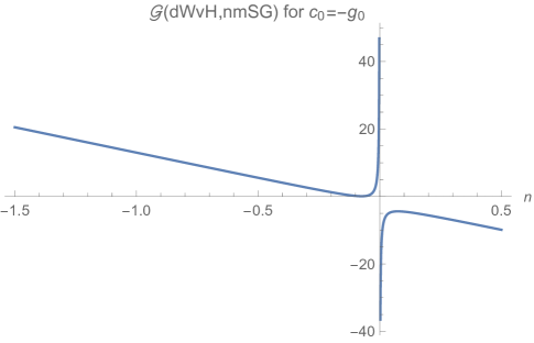
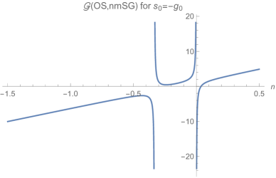
Figure 7: The gadgets $\mathcal{G}(\text{dWvH},\text{{$\not$mSG}})$ and $\mathcal{G}(\text{OS},\text{{$\not$mSG}})$ with $c_{0}=-g_{0}$ and $s_{0}=-g_{0}$.

Finite values of the gadget $\mathcal{G}(\text{dWvH},\text{{$\not$mSG}})$ exist for both $n=-1$ and $n=-1/3$ and a finite value for the gadget $\mathcal{G}(\text{OS},\text{{$\not$mSG}})$ exists for $n=-1$.

$$\mathcal{G}(\text{dWvH},\text{{$\not$mSG}})= ~{}3\left(c_{0}+g_{0}\right){}^{4}+18\left(c_{0}+g_{0}\right){}^{3}+40\left(c_{0}+g_{0}\right){}^{2}+38\left(c_{0}+g_{0}\right)+13~{}\text{for}~{}n=-1$$ (7.42)

$$\mathcal{G}(\text{dWvH},\text{{$\not$mSG}})= ~{}4\left(c_{0}+g_{0}\right){}^{2}+\frac{20}{3}\left(c_{0}+g_{0}\right)+\frac{28}{9}~{}~{}~{}\text{for}~{}~{}~{}n=-1/3$$ (7.43)

$$\mathcal{G}(\text{OS},\text{{$\not$mSG}})= ~{}-3\left(g_{0}+s_{0}\right){}^{3}-12\left(g_{0}+s_{0}\right){}^{2}-15\left(g_{0}+s_{0}\right)-\frac{19}{3}~{}~{}~{}\text{for}~{}~{}~{}n=-1$$ (7.44)

As these results along with Figure 7 indicate, the gadget values between these multiplets can be greater than the normalization of five. This is likely from the non-adinkraic nature of the representations.

8 Conclusions

In this paper, we investigated three different 4D, $\mathcal{N}=1$ SUSY multiplets with 20 boson $\times$ 20 fermion degrees of freedom. Specifically, we investigated two matter gravitino multiplets, dWvH and OS, and non-minimal supergravity ($\not$mSG), each in a one-parameter family of component transformation laws that encode an auxiliary fermion field redefinition symmetry of the diagonal Lagrangian. We furthered research into SUSY genomics and holography by researching the dimensional reduction, $\chi_{0}$ values, and adinkra-level fermionic holoraumy of three $20\times 20$ multiplets. All three have distinct $\chi_{0}$ values. Gadgets calculated between the different multiplets indicate some interesting possible connections to holography. The results in Section 7.2 demonstrate an elegant choice, Equation (7.33), for considering the OS and dWvH multiplets to be parallel in terms of the gadget, that is, have a gadget value of five. Setting either the dWvH and $\not$mSG multiplets parallel or the OS and $\not$mSG multiplets parallel requires specific values of the supergravity parameter $n$ to be selected. On the other hand, no real solutions exist that set the dWvH and OS multiplets orthogonal; however, at least one elegant solution exists that simultaneously sets both the dWvH and OS multiplets to be orthogonal to the $\not$mSG multiplet. These results point to the possibility that holoraumy and the gadget at the adinkra level indicate that the dWvH and OS multiplets are similar in some way, which we know in higher dimensions to be the case as they encode the same dynamical spins of $(3/2,1)$.

Furthermore, fermionic holoraumy and the gadget seem to point to an adinkra-level distinction between the dWvH and $\not$mSG multiplets and the OS and $\not$mSG multiplets. We know of course that a key difference in 4D, $\mathcal{N}=1$ is that the dynamical fields of the $\not$mSG  multiplet have spins $(2,3/2)$ rather than $(3/2,1)$ of the matter gravitino multiplets. We pointed out some features of the gadgets for values of the supergravity parameter $n=-1$, $n=-1/3$ and $n=0$ which correspond to cases where $\not$mSG  becomes part of a tower of higher spin that extends to $\mathcal{N}=2$ SUSY  [?,?,?,?,?], reduces to old-minimal supergravity  [?], and reduces to new-minimal supergravity  [?], respectively.

A precise relationship between fermionic holoraumy and the gadget and spin of the higher dimensional system is still unknown. We look to uncover such precise spin–holography relationships not only through more research of these $20\times 20$ multiplets, but also into $12\times 12$ multiplets of 4D, $\mathcal{N}=1$ supersymmetry, as well as higher spin mutliplets as in  [?,?,?,?]. There are four $12\times 12$ representations of 4D, $\mathcal{N}=1$ off-shell supersymmetry, and of these only one (CLS) has the fermionic auxiliary field redefinition symmetry similar to that presented in this work. This analysis is already being done and we hope to complete it soon. In addition, it would be interesting to see what other gadgets, such as those described in  [?,?], encode for the $12\times 12$, $20\times 20$, and higher spin multiplets. In future works, with the $12\times 12$ and higher spin multiplets, we look for more data to use with the $20\times 20$ gadget data presented in this work to fix a canonical nodal field definition convention that remains consistent among all multiplets and perhaps to fix the diagonal Lagrangian parameters that will continue to be present in higher spin multiplets.

“The most effective way to do it, is to do it.”
 
                                                                                                         -   Amelia Earhart

Acknowledgments
This work was partially supported by the National Science Foundation grant PHY-1315155. This research was also supported in part by the University of Maryland Center for String & Particle Theory (CSPT). K.S. thanks Northwest Missouri State University for computing equipment and travel funds, and Dartmouth College and the E.E. Just Program for hospitality and travel funds that supported this work. K.S. thanks Stephen Randall for work done on the dWvH multiplet while at the University of Maryland. The authors also thank Konstantinos Koutrolikos for many helpful discussions throughout this work and S.J. Gates, Jr. for discussions and for providing the conceptual ideas that led to this work.

Appendix A Proof That $t_{\rm IJ}=1/2{{\boldsymbol{\rm V}}}_{{\rm I}{\rm J}}$ Satisfies the $so(N)$ Algebra

Swapping ${{\boldsymbol{\rm L}}}_{\rm I}$ with ${{\boldsymbol{\rm R}}}_{\rm I}$ interchanges ${{\boldsymbol{\rm V}}}_{{\rm I}{\rm J}}$ with ${{\boldsymbol{\widetilde{\rm V}}}}_{{\rm I}{\rm J}}$, thus proving that $t=1/2{{\boldsymbol{\rm V}}}_{{\rm I}{\rm J}}$ satisfies the $so(N)$ algebra necessarily means that $t=1/2{{\boldsymbol{\widetilde{\rm V}}}}_{{\rm I}{\rm J}}$ must also satisfy the $so(N)$ algebra. We therefore prove the latter, and the former follows by extension. Substituting $t=1/2{{\boldsymbol{\rm V}}}_{{\rm I}{\rm J}}$ into the $so(N)$ algebra, Equation (7.17), results in

$$[{{\boldsymbol{\rm V}}}_{\rm IJ},{{\boldsymbol{\rm V}}}_{\rm KL}]~{}=~{}2i(\delta_{\rm I[L}{{\boldsymbol{\rm V}}}_{\rm K]J}-\delta_{\rm J[L}{{\boldsymbol{\rm V}}}_{\rm K]I}).$$ (A.1)

We now prove Equation (A.1) using repeated use of the garden algebra, Equation (2.25), rearranged as follows

$${{\boldsymbol{\rm L}}}_{{\rm I}}{{\boldsymbol{\rm R}}}_{{\rm J}}=~{} 2\delta_{{\rm I}{\rm J}}-{{\boldsymbol{\rm L}}}_{{\rm J}}{{\boldsymbol{\rm R}}}_{{\rm I}}.$$ (A.2)

We start by substituting the definition of ${{\boldsymbol{\rm V}}}_{{\rm I}{\rm J}}$, Equation (2.29), into the left hand side of Equation (A.1)

$$[{{\boldsymbol{\rm V}}}_{\rm IJ},{{\boldsymbol{\rm V}}}_{KL}]=~{} {{\boldsymbol{\rm V}}}_{\rm IJ}{{\boldsymbol{\rm V}}}_{\rm KL}-{{\boldsymbol{\rm V}}}_{\rm KL}{{\boldsymbol{\rm V}}}_{\rm IJ}$$ (A.3)

$$=~{} -\frac{1}{4}\left({{\boldsymbol{\rm L}}}_{[{\rm I}}{{\boldsymbol{\rm R}}}_{{\rm J}]}{{\boldsymbol{\rm L}}}_{[{\rm K}}{{\boldsymbol{\rm R}}}_{{\rm L}]}-{{\boldsymbol{\rm L}}}_{[{\rm K}}{{\boldsymbol{\rm R}}}_{{\rm L}]}{{\boldsymbol{\rm L}}}_{[{\rm I}}{{\boldsymbol{\rm R}}}_{{\rm J}]}\right)$$ (A.4)

As an intermediate step, we make repeated use of Equation (A.2) to modify the last term, momentarily neglecting the antisymmetry between the indices ${\rm I}$ and ${\rm J}$ and between ${\rm L}$ and ${\rm K}$

$${{\boldsymbol{\rm L}}}_{{\rm K}}{{\boldsymbol{\rm R}}}_{{\rm L}}{{\boldsymbol{\rm L}}}_{{\rm I}}{{\boldsymbol{\rm R}}}_{{\rm J}}=~{} 2\delta_{{\rm I}{\rm L}}{{\boldsymbol{\rm L}}}_{\rm K}{{\boldsymbol{\rm R}}}_{\rm J}-{{\boldsymbol{\rm L}}}_{\rm K}{{\boldsymbol{\rm R}}}_{\rm I}{{\boldsymbol{\rm L}}}_{\rm L}{{\boldsymbol{\rm R}}}_{{\rm J}}$$ (A.5)

$$=~{} 2\delta_{{\rm I}{\rm L}}{{\boldsymbol{\rm L}}}_{\rm K}{{\boldsymbol{\rm R}}}_{\rm J}-2\delta_{{\rm I}{\rm K}}{{\boldsymbol{\rm L}}}_{\rm L}{{\boldsymbol{\rm R}}}_{\rm J}+{{\boldsymbol{\rm L}}}_{\rm I}{{\boldsymbol{\rm R}}}_{\rm K}{{\boldsymbol{\rm L}}}_{\rm L}{{\boldsymbol{\rm R}}}_{\rm J}$$ (A.6)

$$=~{} 2\delta_{{\rm I}{\rm L}}{{\boldsymbol{\rm L}}}_{\rm K}{{\boldsymbol{\rm R}}}_{\rm J}-2\delta_{{\rm I}{\rm K}}{{\boldsymbol{\rm L}}}_{\rm L}{{\boldsymbol{\rm R}}}_{\rm J}+2\delta_{{\rm J}{\rm L}}{{\boldsymbol{\rm L}}}_{\rm I}{{\boldsymbol{\rm R}}}_{\rm K}-{{\boldsymbol{\rm L}}}_{\rm I}{{\boldsymbol{\rm R}}}_{\rm K}{{\boldsymbol{\rm L}}}_{\rm J}{{\boldsymbol{\rm R}}}_{\rm L}$$ (A.7)

$$=~{} 2\delta_{{\rm I}{\rm L}}{{\boldsymbol{\rm L}}}_{\rm K}{{\boldsymbol{\rm R}}}_{\rm J}-2\delta_{{\rm I}{\rm K}}{{\boldsymbol{\rm L}}}_{\rm L}{{\boldsymbol{\rm R}}}_{\rm J}+2\delta_{{\rm J}{\rm L}}{{\boldsymbol{\rm L}}}_{\rm I}{{\boldsymbol{\rm R}}}_{\rm K}-2\delta_{{\rm J}{\rm K}}{{\boldsymbol{\rm L}}}_{\rm I}{{\boldsymbol{\rm R}}}_{\rm L}+{{\boldsymbol{\rm L}}}_{\rm I}{{\boldsymbol{\rm R}}}_{\rm J}{{\boldsymbol{\rm L}}}_{\rm K}{{\boldsymbol{\rm R}}}_{\rm L}$$ (A.8)

Substituting this back into Equation (A.3) yields

$$[{{\boldsymbol{\rm V}}}_{\rm IJ},{{\boldsymbol{\rm V}}}_{KL}]=-\frac{1}{2} \left(\delta_{{\rm I}[{\rm L}}{{\boldsymbol{\rm L}}}_{{\rm K}]}{{\boldsymbol{\rm R}}}_{\rm J}-\delta_{{\rm J}[{\rm L}}{{\boldsymbol{\rm L}}}_{{\rm K}]}{{\boldsymbol{\rm R}}}_{\rm I}-\delta_{{\rm I}[{\rm K}}{{\boldsymbol{\rm L}}}_{{\rm L}]}{{\boldsymbol{\rm R}}}_{\rm J}+\delta_{{\rm J}[{\rm K}}{{\boldsymbol{\rm L}}}_{{\rm L}]}{{\boldsymbol{\rm R}}}_{\rm I}\right.$$ (A.9)

$$\left.-\delta_{{\rm I}[{\rm L}}{{\boldsymbol{\rm L}}}_{|{\rm J}|}{{\boldsymbol{\rm R}}}_{{\rm K}]}+\delta_{{\rm J}[{\rm L}}{{\boldsymbol{\rm L}}}_{|{\rm I}|}{{\boldsymbol{\rm R}}}_{{\rm K}]}-\delta_{{\rm I}[{\rm K}}{{\boldsymbol{\rm L}}}_{|{\rm J}|}{{\boldsymbol{\rm R}}}_{{\rm L}]}-\delta_{{\rm J}[{\rm K}}{{\boldsymbol{\rm L}}}_{|{\rm I}|}{{\boldsymbol{\rm R}}}_{{\rm L}]}\right)$$ (A.10)

The first and fifth terms combine into a single term with ${{\boldsymbol{\rm V}}}_{\rm KJ}$, the second and sixth into ${{\boldsymbol{\rm V}}}_{\rm KI}$ and so on:

$$[{{\boldsymbol{\rm V}}}_{\rm IJ},{{\boldsymbol{\rm V}}}_{KL}]=~{} ~{}i\left(\delta_{{\rm I}[{\rm L}}{{\boldsymbol{\rm V}}}_{{\rm K}]{\rm J}}-\delta_{{\rm J}[{\rm L}}{{\boldsymbol{\rm V}}}_{{\rm K}]{\rm I}}-\delta_{{\rm I}[{\rm K}}{{\boldsymbol{\rm V}}}_{{\rm L}]{\rm J}}+\delta_{{\rm J}[{\rm K}}{{\boldsymbol{\rm V}}}_{{\rm L}]{\rm I}}\right)$$ (A.11)

$$= ~{}2i\left(\delta_{{\rm I}[{\rm L}}{{\boldsymbol{\rm V}}}_{{\rm K}]{\rm J}}-\delta_{{\rm J}[{\rm L}}{{\boldsymbol{\rm V}}}_{{\rm K}]{\rm I}}\right)$$ (A.12)

QED

Appendix B Explicit ${\rm\textbf{L}}_{\rm I}$ and ${\rm\textbf{R}}_{\rm I}$ Matrices

For the choice $c_{0}$ = 0, the explicit ${\rm\textbf{L}}_{\rm I}$ matrices for the dWvH multiplet are

$$L_{1}=~{} \left(\begin{array}[]{cccccccccccccccccccc}1&0&0&0&0&0&0&0&0&0&0&0&0&1&0&0&0&0&0&0\\ 0&0&0&0&1&0&0&0&0&0&0&0&0&0&0&-1&0&0&0&0\\ 0&0&0&0&0&0&0&0&1&0&0&0&1&0&0&0&0&0&0&0\\ 1&0&0&0&0&0&1&0&0&-1&0&0&0&\frac{1}{2}&0&0&\frac{1}{2}&0&0&0\\ 0&0&0&1&0&1&0&0&0&0&1&0&0&0&\frac{1}{2}&0&0&0&0&\frac{1}{2}\\ 0&0&0&0&0&0&0&0&0&0&0&0&0&0&-\frac{1}{2}&0&0&0&0&\frac{1}{2}\\ 0&1&0&0&0&0&0&-1&1&0&0&0&\frac{1}{2}&0&0&0&0&-\frac{1}{2}&0&0\\ 0&-1&0&0&0&0&0&0&0&0&0&0&-\frac{1}{2}&0&0&0&0&\frac{1}{2}&0&0\\ 0&0&0&0&0&-1&0&0&0&0&0&0&0&0&-\frac{1}{2}&0&0&0&0&-\frac{1}{2}\\ 0&0&0&0&0&0&0&0&0&-1&0&0&0&\frac{1}{2}&0&0&\frac{1}{2}&0&0&0\\ 0&0&-1&0&1&0&0&0&0&0&0&1&0&0&0&-\frac{1}{2}&0&0&\frac{1}{2}&0\\ 0&0&1&0&0&0&0&0&0&0&0&0&0&0&0&\frac{1}{2}&0&0&-\frac{1}{2}&0\\ 0&0&0&0&0&0&1&0&0&0&0&0&0&\frac{1}{2}&0&0&\frac{1}{2}&0&0&0\\ 0&0&0&0&0&0&0&0&0&0&1&0&0&0&\frac{1}{2}&0&0&0&0&\frac{1}{2}\\ 1&0&0&0&0&0&0&0&0&0&0&0&0&\frac{3}{2}&0&0&-\frac{1}{2}&0&0&0\\ 0&0&0&0&1&0&0&0&0&0&0&0&0&0&0&-\frac{3}{2}&0&0&-\frac{1}{2}&0\\ 0&0&0&0&0&0&0&0&1&0&0&0&\frac{3}{2}&0&0&0&0&\frac{1}{2}&0&0\\ 0&0&0&0&0&0&0&0&0&0&0&1&0&0&0&-\frac{1}{2}&0&0&\frac{1}{2}&0\\ 0&0&0&1&0&0&0&0&0&0&0&0&0&0&\frac{1}{2}&0&0&0&0&\frac{1}{2}\\ 0&0&0&0&0&0&0&1&0&0&0&0&-\frac{1}{2}&0&0&0&0&\frac{1}{2}&0&0\\ \end{array}\right)$$ (B.21)

$$L_{2}=~{} \left(\begin{array}[]{cccccccccccccccccccc}0&1&0&0&0&0&0&0&0&0&0&0&1&0&0&0&0&0&0&0\\ 0&0&0&0&0&1&0&0&0&0&0&0&0&0&1&0&0&0&0&0\\ 0&0&0&0&0&0&0&0&0&1&0&0&0&-1&0&0&0&0&0&0\\ 0&-1&0&0&0&0&0&1&-1&0&0&0&-\frac{1}{2}&0&0&0&0&\frac{1}{2}&0&0\\ 0&0&1&0&-1&0&0&0&0&0&0&-1&0&0&0&\frac{1}{2}&0&0&-\frac{1}{2}&0\\ 0&0&0&0&0&0&0&0&0&0&0&0&0&0&0&-\frac{1}{2}&0&0&-\frac{1}{2}&0\\ 1&0&0&0&0&0&1&0&0&-1&0&0&0&\frac{1}{2}&0&0&\frac{1}{2}&0&0&0\\ 1&0&0&0&0&0&0&0&0&0&0&0&0&\frac{1}{2}&0&0&\frac{1}{2}&0&0&0\\ 0&0&0&0&1&0&0&0&0&0&0&0&0&0&0&-\frac{1}{2}&0&0&\frac{1}{2}&0\\ 0&0&0&0&0&0&0&0&1&0&0&0&\frac{1}{2}&0&0&0&0&-\frac{1}{2}&0&0\\ 0&0&0&1&0&1&0&0&0&0&1&0&0&0&\frac{1}{2}&0&0&0&0&\frac{1}{2}\\ 0&0&0&1&0&0&0&0&0&0&0&0&0&0&\frac{1}{2}&0&0&0&0&\frac{1}{2}\\ 0&0&0&0&0&0&0&1&0&0&0&0&-\frac{1}{2}&0&0&0&0&\frac{1}{2}&0&0\\ 0&0&0&0&0&0&0&0&0&0&0&1&0&0&0&-\frac{1}{2}&0&0&\frac{1}{2}&0\\ 0&1&0&0&0&0&0&0&0&0&0&0&\frac{3}{2}&0&0&0&0&\frac{1}{2}&0&0\\ 0&0&0&0&0&1&0&0&0&0&0&0&0&0&\frac{3}{2}&0&0&0&0&-\frac{1}{2}\\ 0&0&0&0&0&0&0&0&0&1&0&0&0&-\frac{3}{2}&0&0&\frac{1}{2}&0&0&0\\ 0&0&0&0&0&0&0&0&0&0&-1&0&0&0&-\frac{1}{2}&0&0&0&0&-\frac{1}{2}\\ 0&0&-1&0&0&0&0&0&0&0&0&0&0&0&0&-\frac{1}{2}&0&0&\frac{1}{2}&0\\ 0&0&0&0&0&0&-1&0&0&0&0&0&0&-\frac{1}{2}&0&0&-\frac{1}{2}&0&0&0\\ \end{array}\right)$$ (B.42)

$$L_{3}=~{} \left(\begin{array}[]{cccccccccccccccccccc}0&0&1&0&0&0&0&0&0&0&0&0&0&0&0&1&0&0&0&0\\ 0&0&0&0&0&0&1&0&0&0&0&0&0&1&0&0&0&0&0&0\\ 0&0&0&0&0&0&0&0&0&0&1&0&0&0&1&0&0&0&0&0\\ 0&0&-1&0&1&0&0&0&0&0&0&1&0&0&0&-\frac{1}{2}&0&0&\frac{1}{2}&0\\ 0&-1&0&0&0&0&0&1&-1&0&0&0&-\frac{1}{2}&0&0&0&0&\frac{1}{2}&0&0\\ 0&0&0&0&0&0&0&0&0&0&0&0&\frac{1}{2}&0&0&0&0&\frac{1}{2}&0&0\\ 0&0&0&1&0&1&0&0&0&0&1&0&0&0&\frac{1}{2}&0&0&0&0&\frac{1}{2}\\ 0&0&0&1&0&0&0&0&0&0&0&0&0&0&\frac{1}{2}&0&0&0&0&\frac{1}{2}\\ 0&0&0&0&0&0&0&1&0&0&0&0&-\frac{1}{2}&0&0&0&0&\frac{1}{2}&0&0\\ 0&0&0&0&0&0&0&0&0&0&0&1&0&0&0&-\frac{1}{2}&0&0&\frac{1}{2}&0\\ -1&0&0&0&0&0&-1&0&0&1&0&0&0&-\frac{1}{2}&0&0&-\frac{1}{2}&0&0&0\\ -1&0&0&0&0&0&0&0&0&0&0&0&0&-\frac{1}{2}&0&0&-\frac{1}{2}&0&0&0\\ 0&0&0&0&-1&0&0&0&0&0&0&0&0&0&0&\frac{1}{2}&0&0&-\frac{1}{2}&0\\ 0&0&0&0&0&0&0&0&-1&0&0&0&-\frac{1}{2}&0&0&0&0&\frac{1}{2}&0&0\\ 0&0&1&0&0&0&0&0&0&0&0&0&0&0&0&\frac{3}{2}&0&0&\frac{1}{2}&0\\ 0&0&0&0&0&0&1&0&0&0&0&0&0&\frac{3}{2}&0&0&-\frac{1}{2}&0&0&0\\ 0&0&0&0&0&0&0&0&0&0&1&0&0&0&\frac{3}{2}&0&0&0&0&-\frac{1}{2}\\ 0&0&0&0&0&0&0&0&0&1&0&0&0&-\frac{1}{2}&0&0&-\frac{1}{2}&0&0&0\\ 0&1&0&0&0&0&0&0&0&0&0&0&\frac{1}{2}&0&0&0&0&-\frac{1}{2}&0&0\\ 0&0&0&0&0&1&0&0&0&0&0&0&0&0&\frac{1}{2}&0&0&0&0&\frac{1}{2}\\ \end{array}\right)$$ (B.63)

$$L_{4}=~{} \left(\begin{array}[]{cccccccccccccccccccc}0&0&0&1&0&0&0&0&0&0&0&0&0&0&1&0&0&0&0&0\\ 0&0&0&0&0&0&0&1&0&0&0&0&-1&0&0&0&0&0&0&0\\ 0&0&0&0&0&0&0&0&0&0&0&1&0&0&0&-1&0&0&0&0\\ 0&0&0&1&0&1&0&0&0&0&1&0&0&0&\frac{1}{2}&0&0&0&0&\frac{1}{2}\\ -1&0&0&0&0&0&-1&0&0&1&0&0&0&-\frac{1}{2}&0&0&-\frac{1}{2}&0&0&0\\ 0&0&0&0&0&0&0&0&0&0&0&0&0&\frac{1}{2}&0&0&-\frac{1}{2}&0&0&0\\ 0&0&1&0&-1&0&0&0&0&0&0&-1&0&0&0&\frac{1}{2}&0&0&-\frac{1}{2}&0\\ 0&0&-1&0&0&0&0&0&0&0&0&0&0&0&0&-\frac{1}{2}&0&0&\frac{1}{2}&0\\ 0&0&0&0&0&0&-1&0&0&0&0&0&0&-\frac{1}{2}&0&0&-\frac{1}{2}&0&0&0\\ 0&0&0&0&0&0&0&0&0&0&-1&0&0&0&-\frac{1}{2}&0&0&0&0&-\frac{1}{2}\\ 0&1&0&0&0&0&0&-1&1&0&0&0&\frac{1}{2}&0&0&0&0&-\frac{1}{2}&0&0\\ 0&-1&0&0&0&0&0&0&0&0&0&0&-\frac{1}{2}&0&0&0&0&\frac{1}{2}&0&0\\ 0&0&0&0&0&-1&0&0&0&0&0&0&0&0&-\frac{1}{2}&0&0&0&0&-\frac{1}{2}\\ 0&0&0&0&0&0&0&0&0&-1&0&0&0&\frac{1}{2}&0&0&\frac{1}{2}&0&0&0\\ 0&0&0&1&0&0&0&0&0&0&0&0&0&0&\frac{3}{2}&0&0&0&0&-\frac{1}{2}\\ 0&0&0&0&0&0&0&1&0&0&0&0&-\frac{3}{2}&0&0&0&0&-\frac{1}{2}&0&0\\ 0&0&0&0&0&0&0&0&0&0&0&1&0&0&0&-\frac{3}{2}&0&0&-\frac{1}{2}&0\\ 0&0&0&0&0&0&0&0&-1&0&0&0&-\frac{1}{2}&0&0&0&0&\frac{1}{2}&0&0\\ -1&0&0&0&0&0&0&0&0&0&0&0&0&-\frac{1}{2}&0&0&-\frac{1}{2}&0&0&0\\ 0&0&0&0&-1&0&0&0&0&0&0&0&0&0&0&\frac{1}{2}&0&0&-\frac{1}{2}&0\\ \end{array}\right)$$ (B.84)

The ${\rm\textbf{R}}_{\rm I}$ matrices are inverses of the ${\rm\textbf{L}}_{\rm I}$ matrices: ${\rm\textbf{R}}_{\rm I}={\rm\textbf{L}}_{\rm I}^{-1}$.

Appendix C Explicit Form for the ${{\boldsymbol{\widetilde{\rm V}}}}_{\rm IJ}$ Matrices for the dWVH Multiplet in a $20\times 20$ Tensor Product Basis

It would be instructive to construct a tensor product basis into which $20\times 20$ matrices can be displayed. This is particularly useful for the $\tilde{V}_{\rm IJ}$ matrices, as shown in this section. In  [?], a $so(4)=su(2)\times su(2)$ basis of $4\times 4$ matrices is defined to illustrate how the fundamental adinkras CM, VM, and TM possess this symmetry even at the one-dimensional adinkra level. This $so(4)$ basis is

$$\alpha_{1}= \left(\begin{array}[]{cccc}0&0&0&-i\\ 0&0&-i&0\\ 0&i&0&0\\ i&0&0&0\\ \end{array}\right),~{}~{}~{}\alpha_{2}=\left(\begin{array}[]{cccc}0&-i&0&0\\ i&0&0&0\\ 0&0&0&-i\\ 0&0&i&0\\ \end{array}\right),~{}~{}~{}\alpha_{3}=\left(\begin{array}[]{cccc}0&0&-i&0\\ 0&0&0&i\\ i&0&0&0\\ 0&-i&0&0\\ \end{array}\right)$$

$$\beta_{1}= \left(\begin{array}[]{cccc}0&0&0&-i\\ 0&0&i&0\\ 0&-i&0&0\\ i&0&0&0\\ \end{array}\right),~{}~{}~{}\beta_{2}=\left(\begin{array}[]{cccc}0&0&-i&0\\ 0&0&0&-i\\ i&0&0&0\\ 0&i&0&0\\ \end{array}\right),~{}~{}~{}\beta_{3}=\left(\begin{array}[]{cccc}0&-i&0&0\\ i&0&0&0\\ 0&0&0&i\\ 0&0&-i&0\\ \end{array}\right).$$

These $\beta_{\hat{a}}$ matrices are not to be confused with the auxiliary fermion $\beta_{a}$ for $\not$mSG. In terms of tensor products of Pauli spin matrices $\sigma^{i}$ and the $2\times 2$ identity matrix $I_{2}$, this can be written as

$$\alpha_{1}= \sigma^{2}\otimes\sigma^{1},~{}~{}~{}\alpha_{2}={\rm I}_{2}\otimes\sigma^{2},~{}~{}~{}\alpha_{3}=\sigma^{2}\otimes\sigma^{3}$$

$$\beta_{1}= \sigma^{1}\otimes\sigma^{2},~{}~{}~{}\beta_{2}=\sigma^{2}\otimes{\rm I}_{2},~{}~{}~{}\beta_{3}=\sigma^{3}\otimes\sigma^{2}.$$

Augmenting these six matrices with the $4\times 4$ identity ${\rm I}_{4}$, we construct a sixteen element $l(4,R)$ basis as follows

$${\rm I}_{4},~{}~{}~{}\alpha_{\hat{a}},~{}~{}~{}\beta_{\hat{a}},~{}~{}~{}\alpha_{\hat{a}}\beta_{\hat{b}}.$$ (C.1)

Next, we introduce an $l(5,R)$ basis of $5\times 5$ matrices:

$$\omega_{0}^{5}= \frac{1}{10}{\rm I}_{5},~{}~{}~{}\omega_{1}^{5}=\frac{1}{4}\text{\scriptsize$\left(\begin{array}[]{ccccc}0&1&0&0&0\\ 1&0&0&0&0\\ 0&0&0&0&0\\ 0&0&0&0&0\\ 0&0&0&0&0\\ \end{array}\right)$},~{}~{}~{}\omega_{2}^{5}=\frac{1}{4}\text{\scriptsize$\left(\begin{array}[]{ccccc}0&-1&0&0&0\\ 1&0&0&0&0\\ 0&0&0&0&0\\ 0&0&0&0&0\\ 0&0&0&0&0\\ \end{array}\right)$}$$ (C.12)

$$\omega_{3}^{5}= \frac{1}{4}\text{\scriptsize$\left(\begin{array}[]{ccccc}1&0&0&0&0\\ 0&-1&0&0&0\\ 0&0&0&0&0\\ 0&0&0&0&0\\ 0&0&0&0&0\\ \end{array}\right)$},~{}~{}~{}\omega_{4}^{5}=\frac{1}{4}\text{\scriptsize$\left(\begin{array}[]{ccccc}0&0&1&0&0\\ 0&0&0&0&0\\ 1&0&0&0&0\\ 0&0&0&0&0\\ 0&0&0&0&0\\ \end{array}\right)$},~{}~{}~{}\omega_{5}^{5}=\frac{1}{4}\text{\scriptsize$\left(\begin{array}[]{ccccc}0&0&-1&0&0\\ 0&0&0&0&0\\ 1&0&0&0&0\\ 0&0&0&0&0\\ 0&0&0&0&0\\ \end{array}\right)$}$$ (C.28)

$$\omega_{6}^{5}= \frac{1}{4}\text{\scriptsize$\left(\begin{array}[]{ccccc}0&0&0&0&0\\ 0&0&1&0&0\\ 0&1&0&0&0\\ 0&0&0&0&0\\ 0&0&0&0&0\\ \end{array}\right)$},~{}~{}~{}\omega_{7}^{5}=\frac{1}{4}\text{\scriptsize$\left(\begin{array}[]{ccccc}0&0&0&0&0\\ 0&0&-1&0&0\\ 0&1&0&0&0\\ 0&0&0&0&0\\ 0&0&0&0&0\\ \end{array}\right)$},~{}~{}~{}\omega_{8}^{5}=\frac{1}{12}\text{\scriptsize$\left(\begin{array}[]{ccccc}1&0&0&0&0\\ 0&1&0&0&0\\ 0&0&-2&0&0\\ 0&0&0&0&0\\ 0&0&0&0&0\\ \end{array}\right)$}$$ (C.44)

$$\omega_{9}^{5}= \frac{1}{4}\text{\scriptsize$\left(\begin{array}[]{ccccc}0&0&0&1&0\\ 0&0&0&0&0\\ 0&0&0&0&0\\ 1&0&0&0&0\\ 0&0&0&0&0\\ \end{array}\right)$},~{}~{}~{}\omega_{10}^{5}=\frac{1}{4}\text{\scriptsize$\left(\begin{array}[]{ccccc}0&0&0&-1&0\\ 0&0&0&0&0\\ 0&0&0&0&0\\ 1&0&0&0&0\\ 0&0&0&0&0\\ \end{array}\right)$},~{}~{}~{}\omega_{11}^{5}=\frac{1}{4}\text{\scriptsize$\left(\begin{array}[]{ccccc}0&0&0&0&0\\ 0&0&0&1&0\\ 0&0&0&0&0\\ 0&1&0&0&0\\ 0&0&0&0&0\\ \end{array}\right)$}$$ (C.60)

$$\omega_{12}^{5}= \frac{1}{4}\text{\scriptsize$\left(\begin{array}[]{ccccc}0&0&0&0&0\\ 0&0&0&-1&0\\ 0&0&0&0&0\\ 0&1&0&0&0\\ 0&0&0&0&0\\ \end{array}\right)$},~{}~{}~{}\omega_{13}^{5}=\frac{1}{4}\text{\scriptsize$\left(\begin{array}[]{ccccc}0&0&0&0&0\\ 0&0&0&0&0\\ 0&0&0&1&0\\ 0&0&1&0&0\\ 0&0&0&0&0\\ \end{array}\right)$},~{}~{}~{}\omega_{14}^{5}=\frac{1}{4}\text{\scriptsize$\left(\begin{array}[]{ccccc}0&0&0&0&0\\ 0&0&0&0&0\\ 0&0&0&-1&0\\ 0&0&1&0&0\\ 0&0&0&0&0\\ \end{array}\right)$}$$ (C.76)

$$\omega_{15}^{5}= \frac{1}{24}\text{\scriptsize$\left(\begin{array}[]{ccccc}1&0&0&0&0\\ 0&1&0&0&0\\ 0&0&1&0&0\\ 0&0&0&-3&0\\ 0&0&0&0&0\\ \end{array}\right)$},~{}~{}~{}\omega_{16}^{5}=\frac{1}{4}\text{\scriptsize$\left(\begin{array}[]{ccccc}0&0&0&0&1\\ 0&0&0&0&0\\ 0&0&0&0&0\\ 0&0&0&0&0\\ 1&0&0&0&0\\ \end{array}\right)$},~{}~{}~{}\omega_{17}^{5}=\frac{1}{4}\text{\scriptsize$\left(\begin{array}[]{ccccc}0&0&0&0&-1\\ 0&0&0&0&0\\ 0&0&0&0&0\\ 0&0&0&0&0\\ 1&0&0&0&0\\ \end{array}\right)$}$$ (C.92)

$$\omega_{18}^{5}= \frac{1}{4}\text{\scriptsize$\left(\begin{array}[]{ccccc}0&0&0&0&0\\ 0&0&0&0&1\\ 0&0&0&0&0\\ 0&0&0&0&0\\ 0&1&0&0&0\\ \end{array}\right)$},~{}~{}~{}\omega_{19}^{5}=\frac{1}{4}\text{\scriptsize$\left(\begin{array}[]{ccccc}0&0&0&0&0\\ 0&0&0&0&-1\\ 0&0&0&0&0\\ 0&0&0&0&0\\ 0&1&0&0&0\\ \end{array}\right)$},~{}~{}~{}\omega_{20}^{5}=\frac{1}{4}\text{\scriptsize$\left(\begin{array}[]{ccccc}0&0&0&0&0\\ 0&0&0&0&0\\ 0&0&0&0&1\\ 0&0&0&0&0\\ 0&0&1&0&0\\ \end{array}\right)$}$$ (C.108)

$$\omega_{21}^{5}= \frac{1}{4}\text{\scriptsize$\left(\begin{array}[]{ccccc}0&0&0&0&0\\ 0&0&0&0&0\\ 0&0&0&0&-1\\ 0&0&0&0&0\\ 0&0&1&0&0\\ \end{array}\right)$},~{}~{}~{}\omega_{22}^{5}=\frac{1}{4}\text{\scriptsize$\left(\begin{array}[]{ccccc}0&0&0&0&0\\ 0&0&0&0&0\\ 0&0&0&0&0\\ 0&0&0&0&1\\ 0&0&0&1&0\\ \end{array}\right)$},~{}~{}~{}\omega_{23}^{5}=\frac{1}{4}\text{\scriptsize$\left(\begin{array}[]{ccccc}0&0&0&0&0\\ 0&0&0&0&0\\ 0&0&0&0&0\\ 0&0&0&0&-1\\ 0&0&0&1&0\\ \end{array}\right)$}$$ (C.124)

$$\omega_{24}^{5}= \frac{1}{40}\text{\scriptsize$\left(\begin{array}[]{ccccc}1&0&0&0&0\\ 0&1&0&0&0\\ 0&0&1&0&0\\ 0&0&0&1&0\\ 0&0&0&0&-4\\ \end{array}\right)$}$$ (C.130)

The above basis corresponds to the normalization choice nz[5] = 2 in the data file dWvH.m found at a GitHub data repository, although the user can choose any normalization for any representation. For instance, the form of the first three $l(5,R)$ matrices take the general form

$$\omega_{0}^{5}= \frac{1}{5nz[5]}{\rm I}_{5},~{}~{}~{}\omega_{1}^{5}=\frac{1}{2nz[5]}\text{\tiny$\left(\begin{array}[]{ccccc}0&1&0&0&0\\ 1&0&0&0&0\\ 0&0&0&0&0\\ 0&0&0&0&0\\ 0&0&0&0&0\\ \end{array}\right)$},~{}~{}~{}\omega_{2}^{5}=\frac{1}{2nz[5]}\text{\scriptsize$\left(\begin{array}[]{ccccc}0&-1&0&0&0\\ 1&0&0&0&0\\ 0&0&0&0&0\\ 0&0&0&0&0\\ 0&0&0&0&0\\ \end{array}\right)$}$$ (C.141)

The other $l(5,R)$ matrices have similar generalized normalizations.

For the choice $c_{0}$ = 0 and normalization nz[5] = 2, the explicit form for the ${{\boldsymbol{\widetilde{\rm V}}}}_{\rm IJ}$ matrices for the dWvH multiplet are

$${{\boldsymbol{\widetilde{\rm V}}}}_{\rm 12}= ~{}2i\omega_{9}^{5}\otimes\left(\alpha_{3}\beta_{2}\right)+2i\omega_{10}^{5}\otimes\left(\alpha_{3}\beta_{2}\right)-2i\omega_{13}^{5}\otimes\left(\alpha_{1}\beta_{2}\right)-2i\omega_{14}^{5}\otimes\left(\alpha_{1}\beta_{2}\right)+2i\omega_{16}^{5}\otimes\left(\alpha_{3}\beta_{1}\right)$$ (C.142)

$$+2i\omega_{17}^{5}\otimes\left(\alpha_{3}\beta_{1}\right)-2i\omega_{20}^{5}\otimes\left(\alpha_{1}\beta_{1}\right)-2i\omega_{21}^{5}\otimes\left(\alpha_{1}\beta_{1}\right)-2i\omega_{23}^{5}\otimes\left(\alpha_{2}\beta_{3}\right)+2\omega_{1}^{5}\otimes\alpha_{1}$$ (C.143)

$$+2\omega_{2}^{5}\otimes\alpha_{1}-2\omega_{3}^{5}\otimes\alpha_{2}+2\omega_{6}^{5}\otimes\alpha_{3}-2\omega_{7}^{5}\otimes\alpha_{3}+2\omega_{8}^{5}\otimes\alpha_{2}+5\omega_{15}^{5}\otimes\alpha_{2}+5\omega_{24}^{5}\otimes\alpha_{2}$$ (C.144)

$$-2\omega_{0}^{5}\otimes\beta_{3}+2\omega_{11}^{5}\otimes\beta_{2}-2\omega_{12}^{5}\otimes\beta_{2}+3\omega_{15}^{5}\otimes\beta_{3}+2\omega_{18}^{5}\otimes\beta_{1}-2\omega_{19}^{5}\otimes\beta_{1}$$ (C.145)

$$+3\omega_{24}^{5}\otimes\beta_{3}-4i\omega_{5}^{5}\otimes\text{I}_{4}+2i\omega_{23}^{5}\otimes\text{I}_{4}$$ (C.146)

$${{\boldsymbol{\widetilde{\rm V}}}}_{\rm 13}= -2i\omega_{9}^{5}\otimes\left(\alpha_{2}\beta_{2}\right)-2i\omega_{10}^{5}\otimes\left(\alpha_{2}\beta_{2}\right)+2i\omega_{11}^{5}\otimes\left(\alpha_{1}\beta_{2}\right)+2i\omega_{12}^{5}\otimes\left(\alpha_{1}\beta_{2}\right)$$ (C.147)

$$-2i\omega_{16}^{5}\otimes\left(\alpha_{2}\beta_{1}\right)-2i\omega_{17}^{5}\otimes\left(\alpha_{2}\beta_{1}\right)+2i\omega_{18}^{5}\otimes\left(\alpha_{1}\beta_{1}\right)+2i\omega_{19}^{5}\otimes\left(\alpha_{1}\beta_{1}\right)-2i\omega_{23}^{5}\otimes\left(\alpha_{3}\beta_{3}\right)$$ (C.148)

$$+2\omega_{4}^{5}\otimes\alpha_{1}+2\omega_{5}^{5}\otimes\alpha_{1}+2\omega_{6}^{5}\otimes\alpha_{2}+2\omega_{7}^{5}\otimes\alpha_{2}-4\omega_{8}^{5}\otimes\alpha_{3}$$ (C.149)

$$+5\omega_{15}^{5}\otimes\alpha_{3}+5\omega_{24}^{5}\otimes\alpha_{3}+2\omega_{13}^{5}\otimes\beta_{2}-2\omega_{14}^{5}\otimes\beta_{2}-3\omega_{15}^{5}\otimes\beta_{2}+2\omega_{20}^{5}\otimes\beta_{1}-2\omega_{21}^{5}\otimes\beta_{1}$$ (C.150)

$$-2\omega_{22}^{5}\otimes\beta_{1}+5\omega_{24}^{5}\otimes\beta_{2}+4i\omega_{2}^{5}\otimes\text{I}_{4}$$ (C.151)

$${{\boldsymbol{\widetilde{\rm V}}}}_{\rm 14}= -2i\omega_{11}^{5}\otimes\left(\alpha_{3}\beta_{2}\right)-2i\omega_{12}^{5}\otimes\left(\alpha_{3}\beta_{2}\right)+2i\omega_{13}^{5}\otimes\left(\alpha_{2}\beta_{2}\right)+2i\omega_{14}^{5}\otimes\left(\alpha_{2}\beta_{2}\right)$$ (C.152)

$$-2i\omega_{18}^{5}\otimes\left(\alpha_{3}\beta_{1}\right)-2i\omega_{19}^{5}\otimes\left(\alpha_{3}\beta_{1}\right)+2i\omega_{20}^{5}\otimes\left(\alpha_{2}\beta_{1}\right)+2i\omega_{21}^{5}\otimes\left(\alpha_{2}\beta_{1}\right)-2i\omega_{23}^{5}\otimes\left(\alpha_{1}\beta_{3}\right)$$ (C.153)

$$+2\omega_{1}^{5}\otimes\alpha_{2}-2\omega_{2}^{5}\otimes\alpha_{2}+2\omega_{3}^{5}\otimes\alpha_{1}+2\omega_{4}^{5}\otimes\alpha_{3}-2\omega_{5}^{5}\otimes\alpha_{3}+2\omega_{8}^{5}\otimes\alpha_{1}+5\omega_{15}^{5}\otimes\alpha_{1}$$ (C.154)

$$+5\omega_{24}^{5}\otimes\alpha_{1}+2\omega_{9}^{5}\otimes\beta_{2}-2\omega_{10}^{5}\otimes\beta_{2}+3\omega_{15}^{5}\otimes\beta_{1}+2\omega_{16}^{5}\otimes\beta_{1}-2\omega_{17}^{5}\otimes\beta_{1}-2\omega_{22}^{5}\otimes\beta_{2}$$ (C.155)

$$-5\omega_{24}^{5}\otimes\beta_{1}+4i\omega_{7}^{5}\otimes\text{I}_{4}$$ (C.156)

$${{\boldsymbol{\widetilde{\rm V}}}}_{\rm 23}= -2i\omega_{11}^{5}\otimes\left(\alpha_{3}\beta_{2}\right)-2i\omega_{12}^{5}\otimes\left(\alpha_{3}\beta_{2}\right)+2i\omega_{13}^{5}\otimes\left(\alpha_{2}\beta_{2}\right)+2i\omega_{14}^{5}\otimes\left(\alpha_{2}\beta_{2}\right)$$ (C.157)

$$-2i\omega_{18}^{5}\otimes\left(\alpha_{3}\beta_{1}\right)-2i\omega_{19}^{5}\otimes\left(\alpha_{3}\beta_{1}\right)+2i\omega_{20}^{5}\otimes\left(\alpha_{2}\beta_{1}\right)+2i\omega_{21}^{5}\otimes\left(\alpha_{2}\beta_{1}\right)$$ (C.158)

$$-2i\omega_{23}^{5}\otimes\left(\alpha_{1}\beta_{3}\right)+2\omega_{1}^{5}\otimes\alpha_{2}-2\omega_{2}^{5}\otimes\alpha_{2}+2\omega_{3}^{5}\otimes\alpha_{1}+2\omega_{4}^{5}\otimes\alpha_{3}-2\omega_{5}^{5}\otimes\alpha_{3}$$ (C.159)

$$+2\omega_{8}^{5}\otimes\alpha_{1}+5\omega_{15}^{5}\otimes\alpha_{1}+5\omega_{24}^{5}\otimes\alpha_{1}+2\omega_{9}^{5}\otimes\beta_{2}-2\omega_{10}^{5}\otimes\beta_{2}-3\omega_{15}^{5}\otimes\beta_{1}$$ (C.160)

$$+2\omega_{16}^{5}\otimes\beta_{1}-2\omega_{17}^{5}\otimes\beta_{1}+2\omega_{22}^{5}\otimes\beta_{2}+5\omega_{24}^{5}\otimes\beta_{1}+4i\omega_{7}^{5}\otimes\text{I}_{4}$$ (C.161)

$${{\boldsymbol{\widetilde{\rm V}}}}_{\rm 24}= ~{}2i\omega_{9}^{5}\otimes\left(\alpha_{2}\beta_{2}\right)+2i\omega_{10}^{5}\otimes\left(\alpha_{2}\beta_{2}\right)-2i\omega_{11}^{5}\otimes\left(\alpha_{1}\beta_{2}\right)-2i\omega_{12}^{5}\otimes\left(\alpha_{1}\beta_{2}\right)+2i\omega_{16}^{5}\otimes\left(\alpha_{2}\beta_{1}\right)$$ (C.162)

$$+2i\omega_{17}^{5}\otimes\left(\alpha_{2}\beta_{1}\right)-2i\omega_{18}^{5}\otimes\left(\alpha_{1}\beta_{1}\right)-2i\omega_{19}^{5}\otimes\left(\alpha_{1}\beta_{1}\right)+2i\omega_{23}^{5}\otimes\left(\alpha_{3}\beta_{3}\right)-2\omega_{4}^{5}\otimes\alpha_{1}$$ (C.163)

$$-2\omega_{5}^{5}\otimes\alpha_{1}-2\omega_{6}^{5}\otimes\alpha_{2}-2\omega_{7}^{5}\otimes\alpha_{2}+4\omega_{8}^{5}\otimes\alpha_{3}-5\omega_{15}^{5}\otimes\alpha_{3}-5\omega_{24}^{5}\otimes\alpha_{3}-2\omega_{13}^{5}\otimes\beta_{2}$$ (C.164)

$$+2\omega_{14}^{5}\otimes\beta_{2}-3\omega_{15}^{5}\otimes\beta_{2}-2\omega_{20}^{5}\otimes\beta_{1}+2\omega_{21}^{5}\otimes\beta_{1}-2\omega_{22}^{5}\otimes\beta_{1}+5\omega_{24}^{5}\otimes\beta_{2}$$ (C.165)

$$-4i\omega_{2}^{5}\otimes\text{I}_{4}$$ (C.166)

$${{\boldsymbol{\widetilde{\rm V}}}}_{34}= ~{}2i\omega_{9}^{5}\otimes\left(\alpha_{3}\beta_{2}\right)+2i\omega_{10}^{5}\otimes\left(\alpha_{3}\beta_{2}\right)-2i\omega_{13}^{5}\otimes\left(\alpha_{1}\beta_{2}\right)-2i\omega_{14}^{5}\otimes\left(\alpha_{1}\beta_{2}\right)+2i\omega_{16}^{5}\otimes\left(\alpha_{3}\beta_{1}\right)$$ (C.167)

$$+2i\omega_{17}^{5}\otimes\left(\alpha_{3}\beta_{1}\right)-2i\omega_{20}^{5}\otimes\left(\alpha_{1}\beta_{1}\right)-2i\omega_{21}^{5}\otimes\left(\alpha_{1}\beta_{1}\right)-2i\omega_{23}^{5}\otimes\left(\alpha_{2}\beta_{3}\right)$$ (C.168)

$$+2\omega_{1}^{5}\otimes\alpha_{1}+2\omega_{2}^{5}\otimes\alpha_{1}-2\omega_{3}^{5}\otimes\alpha_{2}+2\omega_{6}^{5}\otimes\alpha_{3}-2\omega_{7}^{5}\otimes\alpha_{3}$$ (C.169)

$$+2\omega_{8}^{5}\otimes\alpha_{2}+5\omega_{15}^{5}\otimes\alpha_{2}+5\omega_{24}^{5}\otimes\alpha_{2}+2\omega_{0}^{5}\otimes\beta_{3}+2\omega_{11}^{5}\otimes\beta_{2}-2\omega_{12}^{5}\otimes\beta_{2}$$ (C.170)

$$-3\omega_{15}^{5}\otimes\beta_{3}+2\omega_{18}^{5}\otimes\beta_{1}-2\omega_{19}^{5}\otimes\beta_{1}-3\omega_{24}^{5}\otimes\beta_{3}-4i\omega_{5}^{5}\otimes\text{I}_{4}-2i\omega_{23}^{5}\otimes\text{I}_{4}$$ (C.171)

Notice that displaying these matrices in this tensor product basis allows displaying about three matrices in the same amount of space where a single $20\times 20$ matrices could be displayed. This is advantageous when matrices have a certain degree of symmetry, as do the ${{\boldsymbol{\widetilde{\rm V}}}}_{\rm IJ}$ holoraumy matrices. The ${{\boldsymbol{\rm L}}}_{\rm I}$ matrices do not have enough symmetry do make displaying them in the tensor product basis particularly advantageous. Nonetheless, representations of all of the ${{\boldsymbol{\rm L}}}_{\rm I}$, ${{\boldsymbol{\rm R}}}_{\rm I}$, ${{\boldsymbol{\rm V}}}_{\rm IJ}$, ${{\boldsymbol{\widetilde{\rm V}}}}_{\rm IJ}$, ${{\boldsymbol{\rm V}}}^{(\pm)}_{\rm IJ}$, and the ${{\boldsymbol{\widetilde{\rm V}}}}^{(\pm)}_{\rm IJ}$ matrices for each of the dWvH, OS, and $\not$mSG  multiplets with arbitrary $c_{0}$, $s_{0}$, and $g_{0}$ parameters in both explicit matrix and tensor product form can be found explicitly within or generated from the file Compare20x20Reps.nb at the previously mentioned GitHub data repository.

References

- [1] Gates, S.J., Jr.; Gonzales, J̇.; MacGregor, B.; Parker, J.; Polo-Sherk, R.; Rodgers, V.G.J.; Wassink, L. 4D, = 1 Supersymmetry Genomics (I). J. High Energy Phys. 2009, 0912, 008.
- [2] Gates, S.J., Jr.; Hallett, J.; Parker, J.; Rodgers, V.G.J.; Stiffler, K. 4D, = 1 Supersymmetry Genomics (II). J. High Energy Phys. 2012, 1206, 071, doi:10.1007/JHEP06(2012)071.
- [3] Chappell, I.; Gates, S.J., Jr.; Linch, W.D.; Parker, J.; Randall, S.; Ridgway, A.; Stiffler, K. 4D, = 1 Supergravity Genomics. J. High Energy Phys. 2013, 1310, 004, doi:10.1007/JHEP10(2013)004.
- [4] Faux, M.; Gates, S.J., Jr. Adinkras: A Graphical technology for supersymmetric representation theory. Phys. Rev. D 2005, 71, 065002, doi:10.1103/PhysRevD.71.065002.
- [5] Doran, C.F.; Faux, M.G.; Gates, S.J., Jr.; Hübsch, T.; Iga, K.M.; Landweber, G.D. On graph-theoretic identifications of Adinkras, supersymmetry representations and superfields. Int. J. Mod. Phys. A 2007, 22, 869–930, doi:10.1142/S0217751X07035112.
- [6] Doran, C.F.; Faux, M.G.; Gates, S.J., Jr.; Hübsch, T.; Iga, K.M.; Landweber, G.D. Adinkras and the Dynamics of Superspace Prepotentials. High Energy Phys. 2006, arXiv:hep-th/0605269.
- [7] Doran, C.F.; Faux, M.G.; Gates, S.J., Jr.; Hübsch, T.; Iga, K.M.; Landweber, G.D.; Miller, R.L. Topology Types of Adinkras and the Corresponding Representations of N-Extended Supersymmetry. arXiv 2008, arXiv:0806.0050.
- [8] Doran, C.F.; Faux, M.G.; Gates, S.J., Jr.; Hübsch, T.; Iga, K.M.; Landweber, G.D.; Miller, R.L. Adinkras for Clifford Algebras, and Worldline Supermultiplets. arXiv 2008, arXiv:0811.3410.
- [9] Douglas, B.L.; Gates, S.J., Jr.; Wang, J.B. Automorphism Properties of Adinkras. arXiv 2010, arXiv:1009.1449.
- [10] Doran, C.F.; Faux, M.G.; Gates, S.J., Jr.; Hübsch, T.; Iga, K.M.; Landweber, G.D.; Miller, R.L. Codes and Supersymmetry in One Dimension. Adv. Theor. Math. Phys. 2011, 15, 1909–1970, doi:10.4310/ATMP.2011.v15.n6.a7.
- [11] Zhang, Y.X. Adinkras for Mathematicians. Trans. Am. Math. Soc. 2014, 366, 3325–3355, doi:10.1090/S0002-9947-2014-06031-5.
- [12] Doran, C.F.; Faux, M.G.; Gates, S.J., Jr.; Hübsch, T.; Iga, K.M.; Landweber, G.D. On the matter of = 2 matter. Phys. Lett. B 2008, 659, 441–446, doi:10.1016/j.physletb.2007.11.001.
- [13] Faux, M. The Conformal Hyperplet. Int. J. Mod. Phys. A 2017, 32, 1750079, doi:10.1142/S0217751X17500798.
- [14] Faux, M.G.; Landweber, G.D. Spin Holography via Dimensional Enhancement. Phys. Lett. 2009, B681, 161–165, doi:10.1016/j.physletb.2009.10.014.
- [15] Faux, M.G.; Iga, K.M.; Landweber, G.D. Dimensional Enhancement via Supersymmetry. Adv. Math. Phys. 2011, 2011, 259089, doi:10.1155/2011/259089.
- [16] Gates, S.J., Jr.; Hübsch, T. On Dimensional Extension of Supersymmetry: From Worldlines to Worldsheets. Adv. Theor. Math. Phys. 2012, 16, 1619–1667, doi:10.4310/ATMP.2012.v16.n6.a2.
- [17] Gates, S.J., Jr. The Search for Elementarity Among Off-Shell SUSY Representations. Korea Inst. Adv. Study Newsl. 2012, 5, 19.
- [18] Gates, S.J., Jr.; Hübsch, T.; Stiffler, K. Adinkras and SUSY Holography: Some Explicit Examples. Int. J. Mod. Phys. 2014, A29, 1450041, arXiv:1208.5999.
- [19] Calkins, M.; Gates, D.E.A.; Gates, S.J.; McPeak, B. Is it possible to embed a supersymmetric vector multiplet within a completely off-shell adinkra hologram? J. High Energy Phys. 2014, 1405, 057, doi:10.1007/JHEP05(2014)057.
- [20] Gates, S.J., Jr.; Hübsch, T.; Stiffler, K. On Clifford-algebraic dimensional extension and SUSY holography. Int. J. Mod. Phys. 2015, A30, 1550042, doi:10.1142/S0217751X15500426.
- [21] Calkins, M.; Gates, D.E.A.; Gates, S.J., Jr.; Stiffler, K. Adinkras, 0-branes, Holoraumy and the SUSY QFT/QM Correspondence. Int. J. Mod. Phys. 2015, A30, 1550050, doi:10.1142/s0217751X15500505.
- [22] Gates, S.J., Jr.; Grover, T.; Miller-Dickson, M.D.; Mondal, B.A.; Oskoui, A.; Regmi, S.; Ross, E.; Shetty, R. A Lorentz covariant holoraumy-induced ’gadget’ from minimal off-shell 4D, = 1 supermultiplets. J. High Energy Phys. 2015, 1511, 113, doi:10.1007/JHEP11.
- [23] Gates, D.E.A.; Gates, S.J., Jr. A Proposal on Culling & Filtering a Coxeter Group for 4D, = 1 Spacetime SUSY Representations. Unpublished work, 2016.
- [24] Gates, D.E.A.; Gates, S.J., Jr.; Stiffler, K. A Proposal on Culling & Filtering a Coxeter Group for 4D, = 1 Spacetime SUSY Representations: Revised. J. High Energy Phys. 2016, 1608, 076, doi:10.1007/JHEP08(2016)076.
- [25] Gates, S.J., Jr.; Guyton, F.; Harmalkar, S.; Kessler, D.S.; Korotkikh, V.; Meszaros, V.A. Adinkras from ordered quartets of BC Coxeter group elements and regarding 1,358,954,496 matrix elements of the Gadget. J. High Energy Phys. 2017, 1706, 006, doi:10.1007/JHEP06(2017)006.
- [26] Gates, S.J.; Iga, K.; Kang, L.; Korotkikh, V.; Stiffler, K. Generating all 36,864 Four-Color Adinkras via Signed Permutations and Organizing into - and -Equivalence Classes. Symmetry 2019, 11, 120, doi:10.3390/sym11010120.
- [27] Gates, S.J.; Kang, L.; Kessler, D.S.; Korotkikh, V. Adinkras from ordered quartets of BC4 Coxeter group elements and regarding another Gadget’s 1,358,954,496 matrix elements. Int. J. Mod. Phys. A 2018, 33, 1850066, doi:10.1142/S0217751X18500665.
- [28] De Wit, B.; van Holten, J.W. Multiplets of Linearized SO(2) Supergravity. Nucl. Phys. 1979, B155, 530–542, doi:10.1016/0550-3213(79)90285-2.
- [29] Fradkin, E.S.; Vasiliev, M.A. Minimal Set of Auxiliary Fields and S Matrix for Extended Supergravity. Lett. Nuovo Cim. 1979, 25, 79–90, doi:10.1007/BF02776267.
- [30] Siegel, W.; Gates, S.J., Jr. (3/2, 1) Superfield of O(2) Supergravity. Nucl. Phys. 1980, B164, 484–494, doi:10.1016/0550-3213(80)90522-2.
- [31] Ogievetsky, V.I.; Sokatchev, E. On Gauge Spinor Superfield. JETP Lett. 1976, 23, 58–59.
- [32] Ogievetsky, V.I.; Sokatchev, E. Superfield Equations of Motion. J. Phys. 1977, A10, 2021–2030.
- [33] Siegel, W.; Gates, S.J., Jr. Superfield Supergravity. Nucl. Phys. 1979, B147, 77–104, doi:10.1016/0550-3213(79)90416-4.
- [34] Zhang, Y.X. A Unified Enumeration of 1-dimension Garden Algebras and Valise Adinkras. arXiv 2018, arXiv:1801.02678.
- [35] Friend, I.; Kostiuk, J.; Zhang, Y.X. Enumerative Gadget Phenomena for -Adinkras. arXiv 2018, arXiv:1810.05545.
- [36] Gates, S.J., Jr.; Kuzenko, S.M.; Sibiryakov, A.G. Towards a unified theory of massless superfields of all superspins. Phys. Lett. B 1997, 394, 343–353, doi:10.1016/S0370-2693(97)00034-8.
- [37] Gates, S.J., Jr.; Koutrolikos, K. On 4D, massless gauge superfields of arbitrary superhelicity. J. High Energy Phys. 2014, 1406, 098.
- [38] Gates, S.J., Jr.; Koutrolikos, K. On 4D, = 1 Massless Gauge Superfields of Higher Superspin: Half-Odd-Integer Case. arXiv 2013, arXiv:1310.7386.
- [39] Gates, S.J., Jr.; Koutrolikos, K. On 4D, = 1 Massless Gauge Superfields of Higher Superspin: Integer Case. arXiv 2013, arXiv:1310.7385.
- [40] Gates, S.J., Jr.; Hallett, J.; Hübsch, T.; Stiffler, K. The Real Anatomy of Complex Linear Superfields. Int. J. Mod. Phys. A 2012, 27, 1250143, doi:10.1142/S0217751X12501436.
- [41] Doran, C.F.; Hübsch, T.; Iga, K.M.; Landweber, G.D. On General Off-Shell Representations of World Line (1D) Supersymmetry. Symmetry 2014, 6, 67–88, doi:10.3390/sym6010067.
- [42] Gates, S.J.; Rana, L. A Theory of spinning particles for large N extended supersymmetry. Phys. Lett. B 1995, 352, 50–58, doi:10.1016/0370-2693(95)00474-Y.
- [43] Gates, S.J., Jr.; Rana, L. A Theory of spinning particles for large N extended supersymmetry(II). Phys. Lett. B 1996, 369, 262–268, doi:10.1016/0370-2693(95)01542-6.
- [44] Georgi, H. Lie algebras in particle physics. Front. Phys. 1999, 54, 1–320.
- [45] Gates, S.J.; Grisaru, M.T.; Rocek, M.; Siegel, W. Superspace or One Thousand and One Lessons in Supersymmetry. Front. Phys. 1983, 58, 1–548.
- [46] Buchbinder, I.L.; Gates, S.J., Jr.; Linch, W.D., III; Phillips, J. New 4-D, = 1 superfield theory: Model of free massive superspin 3/2 multiplet. Phys. Lett. B 2002, 535, 280–288, doi:10.1016/S0370-2693(02)01772-0.