Learning Direct Optimization for Scene Understanding

Abstract

We develop a Learning Direct Optimization (LiDO) method for the refinement of a latent variable model that describes input image $\mathbf{x}$. Our goal is to explain a single image $\mathbf{x}$ with an interpretable 3D computer graphics model having scene graph latent variables $\mathbf{z}$ (such as object appearance, camera position). Given a current estimate of $\mathbf{z}$ we can render a prediction of the image $\mathbf{g}(\mathbf{z})$, which can be compared to the image $\mathbf{x}$. The standard way to proceed is then to measure the error $E(\mathbf{x},\mathbf{g}(\mathbf{z}))$ between the two, and use an optimizer to minimize the error. However, it is unknown which error measure $E$ would be most effective for simultaneously addressing issues such as misaligned objects, occlusions, textures, etc. In contrast, the LiDO approach trains a Prediction Network to predict an update directly to correct $\mathbf{z}$, rather than minimizing the error with respect to $\mathbf{z}$. Experiments show that LiDO converges rapidly as it does not need to perform a search on the error landscape, produces better solutions than error-based competitors, and is able to handle the mismatch between the data and the fitted scene model. We apply LiDO to a realistic synthetic dataset, and show that the method also transfers to work well with real images.

1 Introduction

In this paper we study a Learning Direct Optimization (LiDO) method for the optimization of a latent variable model applied to the problem of explaining an image $\mathbf{x}$ in terms of a computer graphics model.

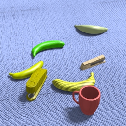
The latent variables (LVs) $\mathbf{z}$ are the scene graph, i.e.: the shape, appearance, position and poses of all objects in the scene, plus global variables such as the camera and lighting. Our work is carried out in an analysis-by-synthesis framework. We develop methods to the problem of scene understanding in 3D from a single image, see Figure 1 — this is to be contrasted with methods that simply predict image-based bounding boxes or pixel labelling. Due to the interpretable 3D representation, one could easily edit the scene, e.g. refine object positions or their colours, or analyse the 3D scene, e.g. compute possible paths so as not to collide with the objects present in the scene.

(a)

(b)

(c)

(d)

Figure 1: (a) Real input image, (b) the rendered image of the 3D scene based on the estimated LVs, (c) the scene under modified illumination and (d) from a different viewpoint.

Given $\mathbf{z}$ we can render the scene graph to obtain a predicted image $\mathbf{g}(\mathbf{z})$, which can be compared to $\mathbf{x}$. The usual way to improve the match is to measure the error $E(\mathbf{x},\mathbf{g}(\mathbf{z}))$, and to use an optimizer to update $\mathbf{z}$ via minimization of $E(\mathbf{x},\mathbf{g}(\mathbf{z}))$. The Learning Direct Optimization approach is based on the idea that we can train a network to predict an update for $\mathbf{z}$ rather than requiring an error measure $E$ to be defined in the image space, and then minimizing it.

The structure of the paper is as follows: in Section 2 we explain LiDO and how it contrasts to error-based optimization, and provide a list of our contributions. In Section 3 we discuss related work. In Section 4 we describe the latent variables, and the initialization networks in Section 5. Section 6 gives details of the experimental datasets. Section 7 provides the details of the setup of error-based optimization, and Section 8 gives the details of LiDO setup and network architecture. Finally, Section 9 describes our evaluation measures, with the results presented in Section 10.

2 Learning Direct Optimization

Figure 2 gives an overview of the Learning Direct Optimization framework.

Figure 2: Learning Direct Optimization: given the observed image $\mathbf{x}$, the initialization of the latent variables (LVs) $\mathbf{z}$ is obtained – then $\mathbf{z}$, the predicted image $\mathbf{g}(\mathbf{z})$ and the observed image $\mathbf{x}$ serve as the input to the LiDO Prediction Network. The LVs are then updated according to the prediction and a new render is produced. The LVs are then refined iteratively driven by the Prediction Network.

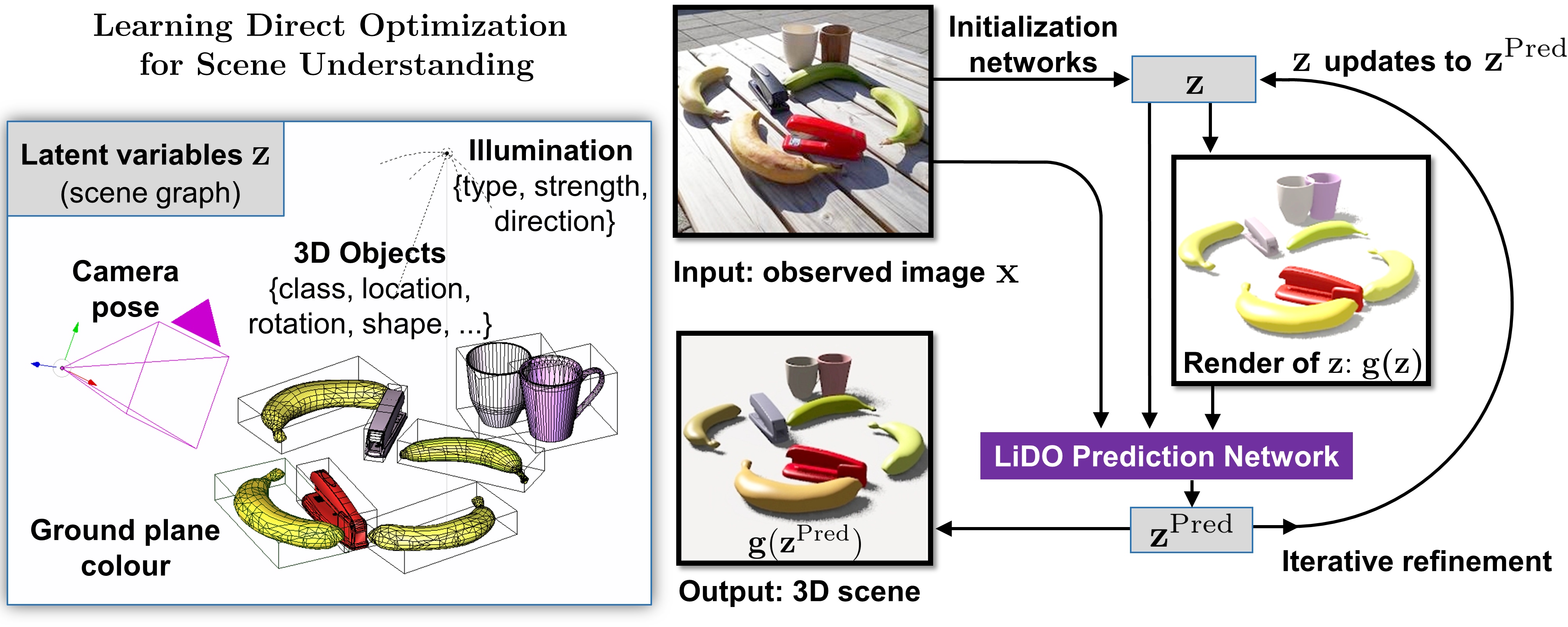
In our system we use initialization networks to predict the starting configuration $\mathbf{z}_{0}$ based on $\mathbf{x}$, which also serves as the initialization for all the compared methods. The representation of the LVs consists of global and object LVs and is of variable dimension, i.e. $\mathbf{z}=(\mathbf{z}^{\mathrm{Global}},\mathbf{z}_{1}^{\mathrm{Object}},\ldots,\mathbf{z}_{P}^{\mathrm{Object}})$, thus initialization networks can initialize an arbitrary number of objects. The initialization networks are described in Sections  4 and 5 below.

Our setup can be viewed as a kind of image autoencoder, with the initialization networks being the encoder, the bottleneck consisting of the LVs $\mathbf{z}$, and the graphics renderer being the decoder. The optimization of $\mathbf{z}$ to improve the fit to the image is non-standard in autoencoders.

The LiDO method trains the Prediction Network on data where the current state $\mathbf{z}$ does not match the ground truth $\mathbf{z}_{GT}$. This was obtained in two ways: (i) from the initialization network where, based on $\mathbf{x}$, $\mathbf{z}_{0}$ and $\mathbf{g}(\mathbf{z}_{0})$, one can predict $\mathbf{z}_{GT}$, and (ii) by perturbing $\mathbf{z}_{GT}$ to produce $\mathbf{z}^{\prime}$, and learning to predict $\mathbf{z}_{GT}$ given $\mathbf{x}$, $\mathbf{z}^{\prime}$ and $\mathbf{g}(\mathbf{z}^{\prime})$. Note that the training data requirements for Prediction Network are similar to that needed to train the initialization networks, and reuse the same data generator, so it has minimal marginal cost.

Given our initial prediction $\mathbf{z}_{0}$, a standard optimization would make steps based on some error $E$ where $E(\mathbf{x},\mathbf{g}(\mathbf{z}_{t}))$ measures the error between the image $\mathbf{x}$ and the current prediction $\mathbf{g}(\mathbf{z}_{t})$. To perform the optimization, one can use a gradient-based optimization (GBO). However, due to the difficulties in obtaining gradients from a renderer, much work for minimizing $E(\mathbf{x},\mathbf{g}(\mathbf{z}))$ has used gradient-free local search methods such a Simplex search, coordinate descent, genetic algorithms [2], or the COBYLA algorithm (as used in [3]).

However, it is unknown which error measure $E$ would be most effective for simultaneously addressing issues such as misaligned objects, occlusions, textures, etc. In contrast, Learning Direct Optimization procedure takes as input $\mathbf{x}$, $\mathbf{z}_{t}$, and the current prediction $\mathbf{g}(\mathbf{z}_{t})$, as shown in Figure 2, and is trained to predict $\mathbf{z}^{\mathrm{pred}}_{t+1}$, the true latent variables corresponding to $\mathbf{x}$, as described in Section 8.

The key insight is that comparison of $\mathbf{x}$ and the render $\mathbf{g}(\mathbf{z}_{t})$ may yield much more information than simply the value of the error measure $E$. For example, consider a scene $\mathbf{x}$ containing a mug viewed from above. If the prediction of $\mathbf{z}_{t}$ has the overall size and position of the mug correct, but the pose is incorrect so that the mug handle is in the wrong place, a comparison of the two images (e.g. by subtraction) will show up a characteristic pattern of differences which can lead to a large move in $\mathbf{z}$ space. In contrast, if the handle positions are far apart, a small change its position will not change the error at all, so there is zero gradient. Indeed this error will not change until there is an overlap between the predicted and observed handles.

Another problem is that the optimization may be misled when the observed image contains noisy features in a form of object textures, shadows, etc., while LiDO Prediction Network can learn to ignore such distractions.

Our contributions are:

1. We develop a general framework for the joint refinement of all the considered LVs in a multi-object scene, including the shape and appearance of the objects, illumination and camera variables, without the need to choose a specific error metric $E$ to measure of the mismatch between the input image and the predicted image.

2. We show that LiDO generally produces better solutions in shorter time and is more stable than standard optimizers, since the $\mathbf{z}$-update directly targets the optimal $\mathbf{z}$ rather than simply moving downhill.

3. We show that LiDO is better able to handle mismatch between the data generator and the fitted scene model, in terms of synthetic vs. real images mismatch, object shape mismatch, and mismatch due to the texture and other nuisance variables.

3 Related Work

The task of scene understanding is a long-standing problem in the computer vision literature, for which various approaches have been developed. In recent years there has been an emphasis on methods which make predictions in the image frame. These include object detection methods which output bounding-boxes (e.g. Selective Search method [4], and YOLO network [5]), object instance segmentation [6] and semantic pixel labelling, e.g. [7], [8]. An older viewpoint in computer vision focuses on recovering 3D geometry of the world from one of more images, such as the work of Marr and Nishihara [9]. Malik et al. [10] discuss the three “R’s” of Recognition (object detection), Reconstruction (inverse graphics) and Reorganization (perceptual organization); they show how these three components can interact to aid each other for scene understanding. Recent work on this theme includes pixel depth prediction [11]; exploiting 3D geometry by placing object detections into perspective at predicted scale and depth [12]; and representing an indoor scene by furniture items described by 3D bounding-boxes [13].

Our work is carried out in the vision-as-inverse-graphics (VIG) or analysis-by-synthesis paradigm, where the vision task is the inverse of the rendering process. This approach not only extracts a 3D scene from the input image, but renders that scene to allow comparison with the input image. VIG is a long-standing idea, see [14] and [2], but it can be reinvigorated using the power of deep learning for the analysis stages. VIG can be broken down into an initialization phase, and a subsequent refinement phase. Williams et al. [15] is an early example of using neural networks for the initialization phase. More recent work includes [16] and [17] who train autoencoders for this task on face data.

The standard practice for refinement after the initialization is to minimize some error function $E$, where the reconstruction loss is based on a summary statistics of the image pixels. The error could, for example, measure the discrepancy in pixel space, or in some other feature space like the representation obtained in higher layers of a neural network (see e.g. [18]). In contrast, LiDO directly predicts updates for all different kinds of LVs together, without the need to chose a specific error metric $E$.

Refinement within the VIG paradigm has also been considered by several works focusing on the specific problem of face explanation. This is a significantly simpler problem for optimization than multi-object scene explanation, as the face (a single object) is always present in the centre of the image and can be modelled by a single deformable mesh. Yildirim et al. [19] use a pixel-based error measure when sampling parameters of a 3D face model; and Schönborn et al. [20] develop a sampling procedure over the probabilistic parameters of the face shape and appearance model. Hu et al. [21] split the problem into simpler sub-tasks and sequentially optimize the pose, shape, light and texture parameters.

For multiple objects the problem is much more challenging, even in 2D, as illustrated by [22] who compare various compute-intensive MCMC methods for the relatively simple problem of fitting multiple colourful 2D squares. For 3D objects, most of the methods match only the 3D geometry to the image via slow sampling procedures. For instance Satkin et al. [23] match 3D CAD models based on a set of various similarity measures calculated using predicted surface normals, detected edges, rendered object mask etc.; the IM2CAD method [3] aligns object shapes to the observed image by minimizing the distance in the VGG feature space; and Zou et al. [24] optimize object poses to fit to the depth channel input by enumerating a large number of object shapes and poses. Note these methods optimize only the geometry, and none of them model the appearance or illumination (for visualizations, objects are given a colour in a post-processing step). Finally, some works consider toy synthetic scenes, but these approaches have only been demonstrated for scenes containing known objects with fixed sizes and appearance (e.g. [25] who consider three objects of a fixed colour, and [26] who consider scenes with objects from the Minecraft game), and hence have not demonstrated applicability to real images.

LiDO not only fits shapes and poses to the image, but makes use of a whole render of a reconstructed 3D scene, and refines all scene graph LVs jointly. This idea of making use of the current render of the scene, falls into the area of “auto context”, which relates to feeding the output of a learning machine to the input to improve results and make use of context information. This was studied e.g. by Tu et al. [27] who used a mask of current pixel labelling to help to improve the segmentation. There is very recent work by Manhardt et al. [28] and the DeepIM method [29] which describe a special case of LiDO as applied to object 6D pose estimation (3D translation plus 3D rotation). In these papers a neural network makes iterative updates to the pose parameters, based on the input image and a render of the current estimate, but only for a known, specific object of a fixed size. In addition, LiDO can handle novel instances at test time, allowing for variable object size, shape, and texture.

4 Latent Variables

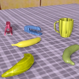
Our work below considers high resolution scenes with a number of objects (from a known set of object classes) on a ground plane (table-top). See Figure 3 for the diagram of the latent variables and example images.

Figure 3: Top: Diagram of the latent variables; bottom: examples from the Synthetic dataset, featuring a variablity in the objects present, their poses, appearance, as well as variable illumination and viewpoints.

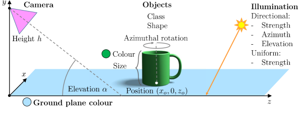
The object LVs are as follows: for each object $o$ its associated LVs are its class $c_{o}$, position $(x_{o},0,z_{o})$ on the ground plane, size $s_{o}$, angle of azimuthal rotation $\phi_{o}$, shape (1-of-$K$ encoding) and colour (RGB).

The global LVs are as follows: ground plane RGB colour, camera LVs and illumination LVs. The camera is taken to be at height $y=h$ above the origin of the $(x,z)$ plane, and to be looking at the ground plane with angle of elevation $\alpha$, with fixed camera intrinsic parameters. The illumination model is uniform lighting (LV: strength) plus a directional source (LVs: strength, azimuth and elevation of the source).

The rendered objects and the ground plane have random noisy textures, and the background is a real indoor image from NYU Depth Dataset V2 [30].

The 1-out-of-K object shape encoding is a simple yet effective shape model. As the predictions are made per detected object and per object class, one could extend this to use e.g. shape and texture morphable models like Blanz and Vetter [31] or later work. However, note that the contribution of our system is demonstrating strong performance on optimizing multiple objects in a complex scene (plus camera, illumination), not just one object.

5 Initialization Networks

Our method uses a separate network (Initialization Network) to provide a first estimate $\mathbf{z}_{0}$ of the values of the LVs that will be then refined.

In our framework we define the object “central contact point” to be the point located at the origin of the CAD object where it is placed on the ground plane. The azimuthal rotation is specified around the vertical axis that passes though the central contact point.

The steps in obtaining an initial scene description are:

1. Detect objects: class, central contact point and size; extract patches $\mathbf{P}^{\mathbf{x}}_{0}$ from input image $\mathbf{x}$ at the central contact points.

2. For each patch $\mathbf{P}^{\mathbf{x}}_{0;p}$ with $p=1,\ldots P$ predict global LVs and object LVs: $\mathbf{z}_{0;p}=({\mathbf{z}_{0;p}^{\mathrm{Global}},\mathbf{z}_{0;p}^{\mathrm{Object}}})$ – global LVs are predicted by each object.

3. Aggregate votes for global LVs to obtain:
   $\mathbf{z}_{0}=(\mathbf{z}_{0}^{\mathrm{Global}},\mathbf{z}_{0;1}^{\mathrm{Object}},\ldots,\mathbf{z}_{0;P}^{\mathrm{Object}}).$

The above steps make use of the detector and LV initialization networks described below, for each patches are of size 128$\times$128 pixels. All the convolutional networks are trained on top of all the 13 convolutional layers of VGG-16 network [32], so as to afford transfer to work on real images.

Object detector: The detector is trained to predict whether a particular object class is present at a given location, together with object size. Trained object detectors are run over the input image to produce a set of detections, which are then sparsified using non-maximum suppression (NMS).

LV initialization networks: We extract an image patch centred at each object detection, and use this to predict the ground truth latent variables. The networks are applied individually to each detected object patch. All the objects predict their own LVs as well as all global LVs. All the global LVs are trained/predicted per object, then combined; for robustness, the aggregation is carried out using the median function.

C gives the details of the network architecture, implementation and training. An important aspect of the architecture is that for azimuthal rotation, we predict the rotation discretized into 18 bins of 20 degrees (the LiDO network predicts the updates in a similar manner, discretized into smaller, 1 degree bins). This allows multimodal predictions and thus the networks can handle the symmetries. For example for a cube object, the network should predict 4 bins every 90-degrees with similar probability, initialize at one of these, and then refine the remaining misalignment.

The outputs of the above stages are assembled into a scene graph. The central contact points of the detected objects are back-projected into a 3D scene given the predicted camera to obtain the 3D positions. The object scaling factors are obtained from the predicted object size and the actual distance from the camera to the object after back-projection.

6 Stochastic Scene Generator and Experimental Datasets

This section present the details of the Stochastic Scene Generator (Section 6.1), the training and test datasets (Sections 6.2, 6.3), and the quality of the initialization (Section 6.4).

6.1 Stochastic Scene Generator

For each image we sample the global LVs and the LVs of up to 7 objects which lie on the ground plane. We consider three object classes: mugs, bananas and staplers. For each object we sample its class, shape (one-of-$K$ = 6/15/8 shapes respectively), colour, rotation, and scaling factor. Since our goal is to apply our networks to real images, the synthetic images are generated with a rich realistic Blender renderer, where we have added shadows, realistic backgrounds and textures on the objects. The textures serve as a noise to allow LiDO to work with richer real images that may feature different kinds of surface patterns, shadows and noise. Textures are applied at a random scaling on the surface via multiplication of the initial colour and the texture intensity. Since we do not model the textures, the mean effect of texture is absorbed into the ground truth (GT) colour. We define the GT colour to be the one that the best matches the texture, i.e. the mean colour of the texture. For example for the white object in black dots, the ground truth colour will be light-grey.

The synthetic images generated by the stochastic scene generator are rendered at 256$\times$256 pixels. We sample the camera height and elevation uniformly in the appropriate ranges: $\alpha\in[0^{\circ},75^{\circ}]$, $h\in[5,75]$ cm. Illumination is represented as uniform lighting plus a directional source, with the strength of the uniform light $\in[0,1]$, the strength of the directional light $\in[0,2]$, with azimuth $\in[0^{\circ},360^{\circ}]$ and elevation $\in[0^{\circ},90^{\circ}]$ of the directional light.

To sample a scene we first select a target number of objects (between four and seven). We then sample the camera parameters and the plane colour. Objects are added sequentially to the scene, and a new object is accepted if at least a half of it is present in the image, it does not intersect other objects, and is not occluded by more than 50%. If it is not possible to place the target number of objects in the scene (e.g. when a camera is pointing downwards from a low height) we reject the scene. For each object we sample its class (stapler, mug or banana), shape, colour, rotation, and scaling factor so that stapler length is $\in[12,16]$cm, mug diameter in $\in[7,10]$cm, banana length $\in[15,20]$cm.

Below we describe the process of sampling realistic colours for our scenes. Initially we experimented with sampling from a uniform distribution but it often results in pastel colours, close to gray. Therefore we use a collection of 17 predefined CSS/HTML colours and sample a pair of them with a random mixing proportion. This samples a variety of colours with frequent strong colours (where the RGB value is either close to 0 or 1), as these are common choices for everyday objects. Afterwards, we add a uniform noise of $\pm 0.2$ to the RGB coefficients and clip if necessary. We use this scheme to sample colours of staplers and mugs, for bananas we fix one of the components to be yellow, for ground plane colours we fix one of the components to be white so as to obtain bright colours more frequently.

6.2 Training Datasets

We train the initialization networks on a dataset of 10,000 images with over 55,000 objects. To train the Prediction Network we use data from two sources. The first (another 10,000 images and over 55,000 objects) is obtained from the $\mathbf{z}_{0}$ outputs of the initialization networks. We paired the detected and GT objects based on the distance of the object central contact points to the closest one of the same class within the radius of 10% of the image width (15% for real images since manual annotations are more noisy than the perfect synthetic ones). The second source was a dataset generated by adding a small amount of noise to 10,000 GT images (over 55,000 objects) to allow LiDO to deal with small errors in further iterations. The noise was uniform for the continuous LVs: $\pm$ the median error made by the initialization networks per LV. We also replaced each GT CAD shape by a random one to train LiDO to work well in the case of shape-mismatch. Thus, the LiDO training dataset consisted of 110,000 object examples.

6.3 Test Datasets

For all the neural networks we used train-validation-test splits of the synthetic dataset, using separate scenes for the Initialization Networks and LiDO Prediction Network. Furthermore, we used a separate validation set for optimization tasks to choose the hyper-parameters of the LiDO and baseline methods, plus a final optimization test set to evaluate them (each of 200 images, with over 1k objects).

Figure 4: Two examples from the Real dataset (images and instance segmentation masks).

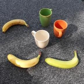
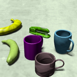
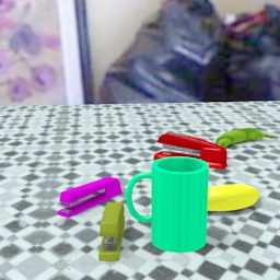
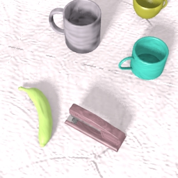
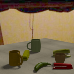
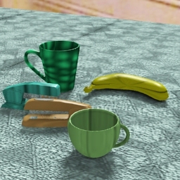
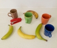
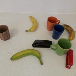
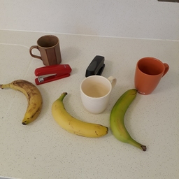
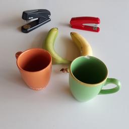
As our aim is to understand real images, we apply the same methods to a dataset consisting of 135 real images with over 750 objects total. The manual annotations are used only for the evaluation, not for making the predictions. The real images were annotated with object masks and central contact points to allow quantitative testing of the methods’ performance, as the quantitative evaluation here can be done only in the pixel space. We captured the real images to feature a number of objects of the considered classes at a variety of lighting, viewpoint and object configuration conditions, see Figure 4. For each object we annotated its class, instance mask, and the central contact point using LabelMe software [35]. Our system renders objects on an infinite ground plane. Since the ground plane is finite for real images, we use a GT ground plane mask that is defined as the ground plane up to a horizontal line located at the central contact point of the farthest GT object. For real images we annotated the GT ground plane mask, since sometimes the mask might not be the full plane.

6.4 Initialization for the Test Datasets

For the synthetic dataset, objects were accurately detected with 94.6% precision, 94.0% recall (94% of objects are detected, 94.6% of all detections are correct), and for these 57% of the object shapes were predicted correctly. For real images, the results were: 97.8% precision, 94.0% recall, showing that the initialization networks worked similarly well for real images. All the methods that we compare start from the same initialization with the same set of the detected objects, and unpaired objects are treated as false positives/negatives. The set of the instantiated objects and their shapes are kept fixed, as these are discrete variables which are not changed during optimization with the above methods.

7 Experimental Setup of Error-Based Optimization

We compare LiDO to two optimization methods: gradient-based optimization (GBO) with the best performing optimizer, and the most effective gradient-free method which was Simplex search (denoted Simp). Note that these baselines were selected as the best-performing methods out of many tested. Since these are standard search methods which require a large number of function evaluations, we use a very fast OpenGL renderer. LiDO was also configured to use OpenGL as the internal renderer during optimization.

For error-based optimization, we compute the match between the actual and rendered image pixels (RGB intensities being between 0 and 1) using a robustified Gaussian likelihood model with standard deviation $\sigma=0.1$ and inlier probability $\alpha=0.8$, as in [36, eq. 3]. The observed image $\mathbf{I}^{O}$ and the rendered image $\mathbf{I}^{R}(\mathbf{x})$ have $P$ pixels and are represented as a vector of a length $3P$, with $P$ values for each RGB colour channel. Then, for each pixel-channel $i$, $p(\mathbf{I}^{O}_{i}|\mathbf{z})$ is given as in [36] by:

$$p(\mathbf{I}^{O}_{i}|\mathbf{z})=\alpha\mathcal{N}({\mathbf{I}}^{O}_{i};{\mathbf{I}}^{R}_{i}(\mathbf{z}),\sigma^{2})+(1-\alpha)\mathcal{U}(\mathbf{I}^{O}_{i}).$$ (1)

For GBO we use a differentiable OpenGL renderer based on OpenDR: Differentiable Renderer [37], extended to simplify rendering multiple objects. The approximate derivatives of the likelihood computed by OpenDR are fed to an optimizer. To facilitate refinement we use anti-aliasing with 8 samples per pixel to make the gradients more accurate and the likelihood function smoother.

We performed experiments with several optimizers and most of them converged poorly (e.g. L-BFGS-B). We found Truncated Newton Conjugate-Gradient (TNC) to considerably outperform other gradient-based methods, with the Nonlinear Conjugate Gradient optimizer being the only other one that usually converged well (yet worse than TNC, so we use TNC for GBO).

For gradient-free methods, we found the Simplex (Nelder-Mead) optimizer worked well and significantly better than COBYLA, Simplex also often performed better and faster than GBO.

Setting proper bounds is crucial for proper optimization as the stepsize is scaled by the distance between LV boundaries, hence for all the LVs we set the bounds to the respective ranges as used in the scene generator.

Following the work of [36], we fit subsets of the search variables sequentially. The LVs are fit in the following order: ground plane colour, object colours (each object separately), object poses (each object separately), illumination and the camera. We experimented with fitting each object’s LVs together, all the object LVs together, and also all LVs together, but it worked a lot less well and overall slower, because the number of variables is larger and likely the optimization landscape is thus more complex.

8 Experimental Setup of Learning Direct Optimization

We ran the initialization networks on the synthetic dataset and took object detections and the associated errors as the new dataset for training LiDO. For an image $\mathbf{x}$ with ground truth $\mathbf{z}_{GT}$ we obtained a set of image patches $\mathbf{P}^{\mathbf{x}}_{0}$ extracted at the object detections and the corresponding rendered patches $\mathbf{P}^{R}_{0}$ from the render $\mathbf{g}(\mathbf{z}_{0})$. From each pair of patches $\mathbf{P}^{\mathbf{x}}_{0;p}$ and $\mathbf{P}^{R}_{0;p}$, $p=1,\ldots,P$ and the corresponding $\mathbf{z}_{0}$ the Prediction Network CNN is trained to predict the object-specific GT variables $\mathbf{z}^{\mathrm{Object}}_{GT;p}$ and the global GT variables $\mathbf{z}^{\mathrm{Global}}_{GT}$. Example errors are that an object could be larger, the camera located higher.

The Prediction Network takes as input both the observed and the rendered image patches (128$\times$128 pixels, down-sampled to 64 by 64 resolution), plus their difference. The RGB channels are stacked together giving an input size of $64\times 64\times 9$. This input is followed by a number of convolutional layers shared across all the LVs. Shared layers are followed by LV-set specific convolutional layers, and finally a few fully-connected layers, each concatenated with the current estimate of $\mathbf{z}_{p}$. For each object patch, the current estimate of $\mathbf{z}_{p}$ (standardized) input consists of: object LVs (discrete class and shape one-hot-encoded), global LVs (as predicted by the object, denoted $G_{O}$), global LVs (as used in the render after voting of all the objects, denoted $G_{V}$), plus their difference $G_{O}-G_{V}$. The whole network for all the LVs is trained together.

To allow convergence, the object pose is trained in the object’s current coordinates/frame (to predict the change in object position and rotation). CNNs are trained together with an L1+L2 error for continuous LVs and categorical cross-entropy for discrete ones. We add the L1 loss to the L2 loss, as when making predictions multiple times small errors aggregate, and L1 appropriately punishes small errors during training. To calculate the overall network loss we sum up each L1+L2 loss and the cross-entropy loss (for which we used a scaling factor 0.2). We use the Adam optimizer with learning rate 0.0003.

We trained the Prediction Network for 20 epochs, this took 15 minutes/epoch on a single GPU. Note that we reuse the same scene generator, and that training time is no more than the training time of the initialization networks.

Afterwards, we run the refinement for $T$ iterations as summarized below:

for $t\in 0$..$(T-1)$:

1. Take patches $\mathbf{P}^{\mathbf{x}}_{t},\mathbf{P}^{R}_{t}$ from the input image $\mathbf{x}$ and the render $\mathbf{g}(\mathbf{z}_{t})$

2. Predict $\mathbf{z}_{t+1;p}^{\mathrm{pred}}$ given each $\mathbf{P}^{\mathbf{x}}_{t;p},\mathbf{P}^{R}_{t;p},\mathbf{z}_{t;p}$ using the Prediction Network
   (clip if outside of the range, e.g. colour not in [0,1]).

3. Update $\mathbf{z}_{t+1;p}=\mathbf{z}_{t;p}+\mu_{t}(\mathbf{z}^{\mathrm{pred}}_{t+1;p}-\mathbf{z}_{t;p})$.

4. Aggregate global LVs to produce $\mathbf{z}_{t+1}$ (in the same manner as in Section 5).

Setting the step size $\mu_{t}=1$ would move from $\mathbf{z}_{t}$ to $\mathbf{z}^{\mathrm{pred}}_{t+1}$, but we have found that in the case of multiple updates, using a $\mu_{t}<1$ which decreases with $t$ leads to better performance than keeping $\mu_{t}$ fixed. We set $\mu_{t}=1/(t+a)$. The hyper-parameter $a=2$ was selected using the validation set split. In the experiments below we run the LiDO iteration for a fixed number of $T=30$ steps to show the convergence curve, but it would be easy to use a termination condition $|\mathbf{z}_{t+1}-\mathbf{z}_{t}|<\epsilon$.

LiDO Prediction Network
Position	Size	Azimuth	Lighting	Camera	Colour (Ob/Gr)
Input $64\times 64\times 9$ (2 images plus their difference, stacked)
C-32-3 (shared)					C-32-3 (stride 2)
C*-64-3 (shared)					C-64-3 (stride 2)
MaxPool-2 (shared)
C*-128-3 (shared)					C*-128-3 (stride 2)
MaxPool-2 (shared)
C*-64-3 (separate per network)
MaxPool-2 (separate per network)
C-32-3 (separate per network)
3 $\times$ Fz-40 (separate per network)					3 $\times$ Fz-40
Fz-2	Fz-1	Softm.(Fz-360)	Fz-5	Fz-2	Fz-3

Table 1: The configurations of the LiDO Prediction Network, the whole network is trained together. Layer description (where N denotes the number of units and K the filter size), is as follows: 1) Convolutional layer: C-N-K; 2) Fully connected layer: F-N; 3) Fully connected layer, with its input concatenated with the current LVs $\mathbf{z}$: Fz-N; 4) Max-pooling layer: MaxPool-K; 5) Softmax output layer on top of a linear layer X: Softm.(X). Non-colour networks: the first 5 layers are shared across all the 5 sub-networks, all the sub-networks on top of them have the same setup. Colour networks are simpler and have fewer layers, and use ReLU activations, while non-colour networks use tanh activations. For lighting we predict: (uniform component strength, directional component: strength, elevation, sin(azimuth), cos(azimuth)). We use dropout with $p=0.5$ after the convolutional layers denoted with *.

Table 1 shows the network configurations used for LiDO. The implementation is in Python (TensorFlow). Again, the region outside the image frame is given as value 0. The [0,255] image dataset values had their mean subtracted and were divided by 100.

When producing the OpenGL renders for the LiDO prediction, we needed to take care because LiDO has been trained to predict $\mathbf{z}$’s that specify a scene for the Blender renderer. While the geometry LVs (objects present, their shape/poses, camera etc.) are common for both the renderers, the optimal colours in OpenGL differ in brightness to Blender, since the OpenGL renderer cannot produce shadows, and has to explain shadowing (e.g. that mugs are dark inside when the light comes from the side) with a lower colour brightness. To render an OpenGL image for the LiDO prediction with Blender colour LVs, we adjust the brightness colour of each object and the ground plane. We do so by scaling the RGB colour by the ratio of the means of brightness calculated at the pixels of the predicted object mask, for LiDO’s OpenGL render and the observed image. We can do this as it uses only the predicted masks, e.g. this would be equivalent to the final iteration of minimizing the MSE w.r.t. the colour LVs.

9 Experimental Evaluation Measures

This section gives the details of the evaluation measures of our interest, in the latent space (Section 9.1) and in the image space (Section 9.2).

9.1 Evaluation of the LVs

For the synthetic dataset, we evaluate the improvement in the LVs for all the methods. We consider suitable evaluation measures specific for the seven different LV-sets, as outlined below.

Object LVs: Object position error is a distance between object central contact points in the image. Object size is the size of the projected object in the image frame, the error is the relative size difference. For azimuthal rotation we measure the absolute angular difference between the prediction and ground truth, but with wrap-around, so the maximum error is $180^{\circ}$. The error metric of the object colour is the RMSE of normalized RGB components (computed as $R/(R+G+B)$ etc.).

Global LVs: Ground plane colour is evaluated as for object colour above. The lighting is projected onto a sphere and evaluated at 313 points uniformly-distributed on the sphere, then normalized; the error is RMSE. To assess the camera error, we place a (virtual) checkerboard in the scene, and compute the RMSE of the errors between the GT and predicted positions of the grid points in the image, as used by [38].

The multiplicative interaction between illumination and colour introduces a problem when evaluating them separately; by using the normalized metrics above we overcome this issue. The joint result of both factors is directly available via pixel intensities (and is compared via MSE).

9.2 Evaluation in the Image Space (2D Projection, Pixels)

We compare the observed and predicted images using the Intersection-over-Union (IoU) of the predicted and GT masks (of objects and ground plane), and MSE of pixel intensities calculated at the GT mask (of objects and ground plane). We can evaluate these measures for both synthetic and real datasets. Note that the IoU of the ground plane assesses differences in the present, missing and superfluous objects. The background (the part of the image not belonging to the ground plane or the object masks) is excluded from the explained pixels. Note that each MSE is calculated at the same pixels for all the methods, as these are calculated only at the GT masks.

10 Results

This section provides the results: Section 10.1 presents the evaluation in terms of the latent variables and shows illustrative examples for the synthetic dataset; Section 10.2 presents the evaluation in the image space for both the synthetic and real datasets, and shows illustrative examples for the real dataset.

Figure 5: Median errors vs time in seconds (top: object LVs, bottom: global LVs). All three methods (GBO, Simp, LiDO) start from the initialization error (Init) located at the black dashed line. Note the rapid convergence of LiDO.

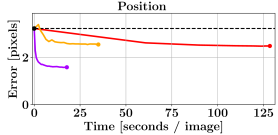
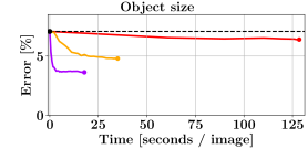
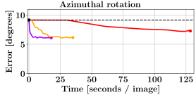
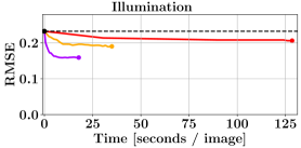
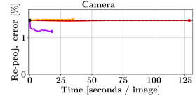
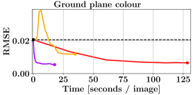
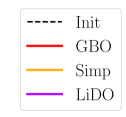
We ran the methods long enough to allow convergence: 50 iterations for GBO, 100 iterations for Simplex, and 30 for LiDO, see Figure 5. All the times shown are for a 4-core CPU for all the methods, to make the comparison fair LiDO is also executed on a CPU, including the CNNs.

Initialization Improvement[%] Impr. hard cases[%] LVs name Err. Unit GBO Simp LiDO GBO Simp LiDO Object position 3.23 pix 22.9 21.0 51.0* 76 71 92 Object colour 0.027 RMSE 14.0 12.4 59.1* 70 67 95 Object size 7.08 % 09.7 32.2 48.7* 72 70 87 Object azimuth 9.15 deg. 20.3 32.6 33.1 62 62 67 Illumination 0.23 RMSE 11.3 18.1 31.6* 75 80 86 Camera 1.47 r.e. 00.3 0-1.3. 20.7* 37 45 80 Ground colour 0.021 RMSE 68.2 42.4 73.6 80 66 92

Table 2: Results of the Initialization (left), “Improvement” (centre) and “Improved hard cases” (right). Initialization: median errors as per the evaluation measures given in Section 9.1, units are: pix – pixels, deg. – degrees, r.e – re-projection error;
Improvement: each value indicates how much (in %) the median error across observations was lower after the refinement compared to the median error of the initialization. Ground truth would give 100% improvement, * denotes a statistically significantly better method.
Improved hard cases: for “hard cases” we considered the worst 50% of the initializations, individually per each LV-set. We show percentage of the hard cases that have been improved (see also plots in Figure 7).

10.1 Results: Evaluation of the LVs on the Synthetic Dataset

Table 2 (centre) shows the percentage improvement of the median error of each of the methods (GBO, Simp, LiDO) over the median error of the initialization (Init, left). For all seven evaluation measures LiDO outperforms both GBO and Simp. For four out of seven LV sets the LiDO improvements are at least two times higher than the competitors (on illumination, camera, object: colour, position). We calculate all the different metrics as in Section 9.1, e.g. deviation in pixels for object position or angle in degrees for rotation. However, since all the LVs are in different units, we compare the percentage improvement over the initialization.

Observed	Initializat.	GBO	Simplex	LiDO	LiDO-R
	\begin{overpic}[width=69.38078pt]{img/imgs/220init} \put(0.0,0.0){\includegraphics[width=69.38078pt]{img/imgs/220CO}} \end{overpic}	\begin{overpic}[width=69.38078pt]{img/imgs/220o} \put(0.0,0.0){\includegraphics[width=69.38078pt]{img/imgs/220CO}} \end{overpic}	\begin{overpic}[width=69.38078pt]{img/imgs/220s} \put(0.0,0.0){\includegraphics[width=69.38078pt]{img/imgs/220CO}} \end{overpic}	\begin{overpic}[width=69.38078pt]{img/imgs/220lgl} \put(0.0,0.0){\includegraphics[width=69.38078pt]{img/imgs/220CO}} \end{overpic}	\begin{overpic}[width=69.38078pt]{img/imgs/220l} \end{overpic}
Good initialization: given a good initialization all the methods usually converge well, e.g. 4 leftmost objects, for the two rightmost objects (mug and banana) where the initialized masks are less accurate, only LiDO fits the colours properly.
	\begin{overpic}[width=69.38078pt]{img/imgs/377init} \put(0.0,0.0){\includegraphics[width=69.38078pt]{img/imgs/377CO}} \end{overpic}	\begin{overpic}[width=69.38078pt]{img/imgs/377o} \put(0.0,0.0){\includegraphics[width=69.38078pt]{img/imgs/377CO}} \end{overpic}	\begin{overpic}[width=69.38078pt]{img/imgs/377s} \put(0.0,0.0){\includegraphics[width=69.38078pt]{img/imgs/377CO}} \end{overpic}	\begin{overpic}[width=69.38078pt]{img/imgs/377lgl} \put(0.0,0.0){\includegraphics[width=69.38078pt]{img/imgs/377CO}} \end{overpic}	\begin{overpic}[width=69.38078pt]{img/imgs/377l} \end{overpic}
Textures and shadows: There are two staplers in the input image and the blue one was not detected as it is hardly visible. For GBO and Simp the pink stapler converges wrongly, and the same happens for the front mug, which enlarges to explain the shadow. LiDO is robust to such distractors, note for these objects the CAD shapes are different than observed.

Figure 6: Example runs for Synthetic dataset, showing from left: the observed input image, the initialization (OpenGL), and images after refinement for GBO, Simplex and LiDO using OpenGL renderers, and LiDO using Blender renderer (LiDO-R). We overlay black contours of the ground truth object masks on top of each OpenGL image to ease the comparison.

To assess the statistical significance we conduct a paired test on the errors derived from each image (for global LVs) or object (for object LVs), using the Wilcoxon signed-rank test, at the significance level 0.05. For these LiDO outperforms GBO for 6 out of 7 LVs, and Simp also for 6 out of 7 LVs. This is because GBO does well with ground-plane colour since the objective it minimizes are the differences in pixel intensities between the input image $\mathbf{x}$ and the render $\mathbf{g}(\mathbf{x})$, and Simp performs similarly to LiDO for the azimuthal rotation, but much worse for all other LVs.

Figure 5 shows the evolution of the median errors over time for the seven error measures; it is notable that LiDO obtains a lower error in much shorter time; for error-based methods since we do iterations sequentially for each object, we report the time for each iteration as the average time of reaching it.

The main reason why LiDO is faster is that it requires only a single render of the scene per update of all the LVs, and all the configurations are accepted. In contrast standard optimizers accept only a fraction of the rendered configurations, as these search over the error landscape and usually need several renders (e.g. within a line search for GBO to choose the step-size) before accepting a new configuration. For our datasets, Simp accepts only approximately 30% of the rendered configurations it investigates, and GBO 7%. Recall also that Simp and GBO update only subsets of $\mathbf{z}$ per search step, as we found (see Section 7) that fitting all LVs together worked less well and was slower overall.

Figure 7: The distribution of the differences of the initial and final errors ($\mathbf{e}_{init}-\mathbf{e}_{final}$) of the methods for each of the seven LV-sets for hard cases – kernel density estimate. Improved cases are on the right of the 0-line, the less mass on the left the better. For all the LV-sets LiDO performs better than the baselines, note LiDO usually has much less mass on the left side of the plot than the baselines.

Figure 6 shows example runs, showing both success and failure cases, see textual descriptions under each image set.

More examples of the fitting are given in A, and the video of the fitting at: https://youtu.be/Axc0G8IggVU.

For evaluating the robustness and convergence of the optimizers, the most interesting cases are the ones for which the initialization is not accurate. We performed an additional study to measure the performance for difficult cases. For such “hard cases” we considered the worst 50% of the initializations, individually per each LV-set, these ranged from average to poor initializations. Since we have 200 test images, for each LV-set we used the worst 50% of initializations so as to keep the sample sizes sufficiently large, this led to 532 object LVs and 100 global LVs.

We calculate the percentage of the hard cases that are improved, these are shown in Table 2 (right). LiDO performs well and much better than the other methods; for 3 out of 7 LV-sets more than 90% cases are improved. For GBO and Simp none of the individual results exceeds 80%.

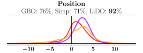
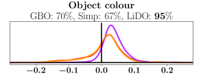
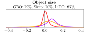
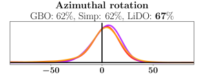
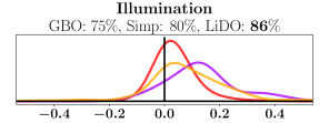
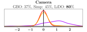
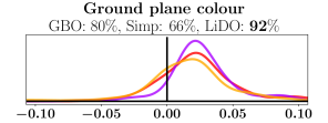
We can get a more fine-grained view of the performance by considering the distribution of the changes of the errors, see Figure 7. For each LV-set and for each method we show the kernel density estimate (KDE) of the distribution of the differences $\mathbf{\Delta}=\mathbf{e}_{init}-\mathbf{e}_{final}$ of the initial and final errors. Values on the right of the vertical line indicate an improvement. For 6 out of 7 LV-sets, LiDO has a much lower amount of mass on the left-hand-side than the baselines. For example, for the Position LVs it is only 8% ($100\%-92\%$), while these are 24% and 29% for GBO and Simp respectively. For the Camera LVs only LiDO makes noticeable improvements. For Azimuthal rotation the performance of all the methods is similar.

10.2 Results: Image-Space Evaluation for the Synthetic and Real Datasets

Results for the Synthetic dataset for image-space measures are given in Table 3. To allow an equal comparison of three optimizers, all three methods use the OpenGL renderer. For all the measures LiDO outperforms the other methods, and particularly LiDO works much better for IoU measures. Note that due to unrealisable textures and shadows, the minimal (OpenGL GT) MSE errors are above 0, these are 11.7 for objects, and 8.4 for the ground plane.

Measure	INIT	GBO	Simp	LiDO
IoU [ob]	66.2	73.1	74.9	78.9*	$\uparrow$
IoU [gr]	86.4	88.7	88.8	91.3*
MSE [ob]	54.1	29.2	26.4	21.8*	$\downarrow$
MSE [gr]	34.1	12.8	13.6	11.90

Table 3: Results of the pixel evaluation for synthetic dataset. Mean IoU (in %) and MSE $(\times 10^{3})$ for the objects [ob] and ground plane [gr]. The arrows indicate whether higher or lower values are better. * denotes a statistically significantly better method, using the Wilcoxon signed-rank test, at the significance level 0.05.

Measure	INIT	GBO	Simp	LiDO
IoU [ob]	60.9	63.2	61.5	71.4*	$\uparrow$
IoU [gr]	87.6	87.3	86.1	91.0*
MSE [ob]	79.1	42.6	46.2	35.9*	$\downarrow$
MSE [gr]	69.1	27.5	30.5	19.2*

Table 4: Results of the pixel evaluation for real dataset. Mean IoU (in %) and MSE $(\times 10^{3})$ for the objects [ob] and ground plane [gr]. * denotes a statistically significantly better method.

Results for Real Dataset are given in Table 4. Since real images are more noisy and difficult, GBO and Simp work poorly for IoU (there is a very minor improvement for objects, and no improvement for the ground plane). All the methods improve the pixel colours (MSE), but note this is because the pixel match is an explicit error measure for GBO and Simp. LiDO, which has been trained on synthetic data, transfers to work better with real images for all four measures.

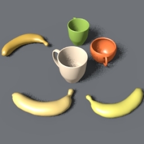
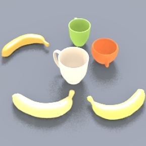
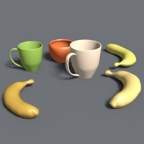
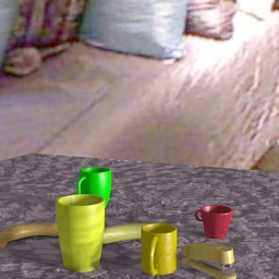
Note the initialized CAD shapes for real images are well matched (see similar object shapes in Figure 8), even though these shapes were never observed during training. The objects and global LVs are then refined well. This was facilitated by introducing shape mismatch in the second noisy dataset source of LiDO (see Section 6.2).

Observed	Initializiat.	GBO	Simplex	LiDO	LiDO-R
	\begin{overpic}[width=69.38078pt,trim=10.03749pt 30.11249pt 0.0pt 20.075pt,clip]{img/imgs_real/76init} \put(0.0,0.0){\includegraphics[width=69.38078pt,trim=10.03749pt 30.11249pt 0.0pt 20.075pt,clip]{img/imgs_real/76CO}} \end{overpic}	\begin{overpic}[width=69.38078pt,trim=10.03749pt 30.11249pt 0.0pt 20.075pt,clip]{img/imgs_real/76o} \put(0.0,0.0){\includegraphics[width=69.38078pt,trim=10.03749pt 30.11249pt 0.0pt 20.075pt,clip]{img/imgs_real/76CO}} \end{overpic}	\begin{overpic}[width=69.38078pt,trim=10.03749pt 30.11249pt 0.0pt 20.075pt,clip]{img/imgs_real/76s} \put(0.0,0.0){\includegraphics[width=69.38078pt,trim=10.03749pt 30.11249pt 0.0pt 20.075pt,clip]{img/imgs_real/76CO}} \end{overpic}	\begin{overpic}[width=69.38078pt,trim=10.03749pt 30.11249pt 0.0pt 20.075pt,clip]{img/imgs_real/76A} \put(0.0,0.0){\includegraphics[width=69.38078pt,trim=10.03749pt 30.11249pt 0.0pt 20.075pt,clip]{img/imgs_real/76CO}} \end{overpic}	\begin{overpic}[width=69.38078pt,trim=10.03749pt 30.11249pt 0.0pt 20.075pt,clip]{img/imgs_real/76l} \end{overpic}
The left-hand banana size and pose is wrong in the Init, only LiDO fits it properly, overall good performance of all the methods, e.g. the left-hand mug obtains brown colour.
	\begin{overpic}[width=69.38078pt,trim=0.0pt 20.075pt 0.0pt 10.03749pt,clip]{img/imgs_real/95init} \put(0.0,0.0){\includegraphics[width=69.38078pt,trim=0.0pt 20.075pt 0.0pt 10.03749pt,clip]{img/imgs_real/95CO}} \end{overpic}	\begin{overpic}[width=69.38078pt,trim=0.0pt 20.075pt 0.0pt 10.03749pt,clip]{img/imgs_real/95o} \put(0.0,0.0){\includegraphics[width=69.38078pt]{img/imgs_real/95CO}} \end{overpic}	\begin{overpic}[width=69.38078pt,trim=0.0pt 20.075pt 0.0pt 10.03749pt,clip]{img/imgs_real/95s} \put(0.0,0.0){\includegraphics[width=69.38078pt,trim=0.0pt 20.075pt 0.0pt 10.03749pt,clip]{img/imgs_real/95CO}} \end{overpic}	\begin{overpic}[width=69.38078pt,trim=0.0pt 20.075pt 0.0pt 10.03749pt,clip]{img/imgs_real/95A} \put(0.0,0.0){\includegraphics[width=69.38078pt,trim=0.0pt 20.075pt 0.0pt 10.03749pt,clip]{img/imgs_real/95CO}} \end{overpic}	\begin{overpic}[width=69.38078pt,trim=0.0pt 20.075pt 0.0pt 10.03749pt,clip]{img/imgs_real/95l} \end{overpic}
Difficult scene, here GBO and Simp diverge objects, LiDO works well (see the gray stapler and the banana near the mugs).
	\begin{overpic}[width=69.38078pt,trim=0.0pt 20.075pt 0.0pt 10.03749pt,clip]{img/imgs_real/97init} \put(0.0,0.0){\includegraphics[width=69.38078pt,trim=0.0pt 20.075pt 0.0pt 10.03749pt,clip]{img/imgs_real/97CO}} \end{overpic}	\begin{overpic}[width=69.38078pt,trim=0.0pt 20.075pt 0.0pt 10.03749pt,clip]{img/imgs_real/97o} \put(0.0,0.0){\includegraphics[width=69.38078pt,trim=0.0pt 20.075pt 0.0pt 10.03749pt,clip]{img/imgs_real/97CO}} \end{overpic}	\begin{overpic}[width=69.38078pt,trim=0.0pt 20.075pt 0.0pt 10.03749pt,clip]{img/imgs_real/97s} \put(0.0,0.0){\includegraphics[width=69.38078pt,trim=0.0pt 20.075pt 0.0pt 10.03749pt,clip]{img/imgs_real/97CO}} \end{overpic}	\begin{overpic}[width=69.38078pt,trim=0.0pt 20.075pt 0.0pt 10.03749pt,clip]{img/imgs_real/97A} \put(0.0,0.0){\includegraphics[width=69.38078pt,trim=0.0pt 20.075pt 0.0pt 10.03749pt,clip]{img/imgs_real/97CO}} \end{overpic}	\begin{overpic}[width=69.38078pt,trim=0.0pt 20.075pt 0.0pt 10.03749pt,clip]{img/imgs_real/97l} \end{overpic}
GBO and Simplex corrupt the initialization, LiDO improves the object poses.
	\begin{overpic}[width=69.38078pt,trim=0.0pt 20.075pt 0.0pt 10.03749pt,clip]{img/imgs_real/114init} \put(0.0,0.0){\includegraphics[width=69.38078pt,trim=0.0pt 20.075pt 0.0pt 10.03749pt,clip]{img/imgs_real/114CO}} \end{overpic}	\begin{overpic}[width=69.38078pt,trim=0.0pt 20.075pt 0.0pt 10.03749pt,clip]{img/imgs_real/114o} \put(0.0,0.0){\includegraphics[width=69.38078pt,trim=0.0pt 20.075pt 0.0pt 10.03749pt,clip]{img/imgs_real/114CO}} \end{overpic}	\begin{overpic}[width=69.38078pt,trim=0.0pt 20.075pt 0.0pt 10.03749pt,clip]{img/imgs_real/114s} \put(0.0,0.0){\includegraphics[width=69.38078pt,trim=0.0pt 20.075pt 0.0pt 10.03749pt,clip]{img/imgs_real/114CO}} \end{overpic}	\begin{overpic}[width=69.38078pt,trim=0.0pt 20.075pt 0.0pt 10.03749pt,clip]{img/imgs_real/114A} \put(0.0,0.0){\includegraphics[width=69.38078pt,trim=0.0pt 20.075pt 0.0pt 10.03749pt,clip]{img/imgs_real/114CO}} \end{overpic}	\begin{overpic}[width=69.38078pt,trim=0.0pt 20.075pt 0.0pt 10.03749pt,clip]{img/imgs_real/114l} \end{overpic}
All the methods update the colours and poses of most of the objects, yet LiDO is much more accurate (for example, compare each of the four bananas). The colours of LiDO of all the objects are well predicted (compare output of each method to the observed image).

Figure 8: Example runs for Real dataset, the order is the same as in Figure 6. Also note that for each image the camera viewpoint is initialized accurately, and how similar the Observed and LiDO-R images are. Obtaining an exact match to the ground truth outline may be impossible because we only have a fixed set of shapes to choose from, none of which may match the actual object shape.

The results in Tables 3 and 4 afford a direct comparison of the optimizers, all using the OpenGL renderer. However, we can also run LiDO with its “native” renderer Blender (shown as the LiDO-R column in Figures 6 and 8). We calculated the MSE errors for Blender renderer (IoUs are the same for both renderers since only the appearance changes). These MSE errors were similar to LiDO that used OpenGL renderer (for Synthetic dataset: 21.6 [ob] and 11.3 [gr], for Real dataset: 40.9 [ob] and 23.0 [gr]).

Figure 8 shows example runs and explanatory text for real image examples. In general LiDO obtains better results in a shorter test-time than the alternatives, and usually converges to a better configuration. LiDO also has the advantage that it can be trained to handle model mismatch, as shown in the real dataset experiments. More examples are given in B.

11 Discussion

Above we have demonstrated LiDO, a full framework for the initialization and refinement of a 3D representation of the scene from a single image. The main features of LiDO are: the advantage of not requiring an error metric $E$ to be defined in image space, rapid convergence, and robust refinement in the presence of noise and distractors. LiDO is generally robust to issues that are common for error-based methods: the updates can point in wrong direction when dealing with cluttered scenes and shadows in observed images; difficulties can arise from an inability to exactly match the target object with one of a different shape; and when predicted objects overlap the background or other objects. LiDO is generally robust to such problems as it directly learns to optimize in the latent space. Our method is not limited to rigid objects, one could use LiDO for e.g. multiple-human pose estimation, or hand-pose and appearance reconstruction.

One apparent limitation of LiDO is that we need to train an additional Prediction Network in advance for a particular dataset. Incorporating neural networks requires extra time for training, but allows for smarter LV updates.

Another potential limitation is a need for a synthetic training dataset. Although such a dataset is required to train the LiDO Prediction Network, for any method one also needs to use an initializer of the scene graph LVs. This means that: i) the initializer was trained already on such dataset, and ii) a 3D graphics representation of a scene graph LVs would be available. This representation and the dataset can be reused for LiDO, e.g. by computing the initialization errors, or by adding noise to the ground truth LVs. The advantages of LiDO mean that it could be a critical component in the development of future vision-as-inverse-graphics systems.

Acknowledgments

We thank the anonymous referees for their comments which have helped improve the paper.

LR was supported by Microsoft Research through its PhD Scholarship Programme. The work of CW was supported in part by The Alan Turing Institute under the EPSRC grant EP/N510129/1.

Appendix A More Examples of Prediction for Synthetic Dataset

Observed	Initializiat.	GBO	Simplex	LiDO	LiDO-R
Poor initialization: GBO and Simplex converge to wrong configurations of object poses and colours, while LiDO is robust to initialization errors; note here the initialized object sizes are wrong and LiDO improves all the detected objects.
	\begin{overpic}[width=69.38078pt]{img/imgs/246init} \put(0.0,0.0){\includegraphics[width=69.38078pt]{img/imgs/246CO}} \end{overpic}	\begin{overpic}[width=69.38078pt]{img/imgs/246o} \put(0.0,0.0){\includegraphics[width=69.38078pt]{img/imgs/246CO}} \end{overpic}	\begin{overpic}[width=69.38078pt]{img/imgs/246s} \put(0.0,0.0){\includegraphics[width=69.38078pt]{img/imgs/246CO}} \end{overpic}	\begin{overpic}[width=69.38078pt]{img/imgs/246lgl} \put(0.0,0.0){\includegraphics[width=69.38078pt]{img/imgs/246CO}} \end{overpic}	\begin{overpic}[width=69.38078pt]{img/imgs/246l} \end{overpic}
Typical input (1): There are 7 objects, 6 object converge properly for all the methods, the initialized position of the bottom banana in wrong, all the methods fail to fix it: GBO and Simplex corrupt the colour, LiDO maintains the yellow colour.
	\begin{overpic}[width=69.38078pt]{img/imgs/273init} \put(0.0,0.0){\includegraphics[width=69.38078pt]{img/imgs/273CO}} \end{overpic}	\begin{overpic}[width=69.38078pt]{img/imgs/273o} \put(0.0,0.0){\includegraphics[width=69.38078pt]{img/imgs/273CO}} \end{overpic}	\begin{overpic}[width=69.38078pt]{img/imgs/273s} \put(0.0,0.0){\includegraphics[width=69.38078pt]{img/imgs/273CO}} \end{overpic}	\begin{overpic}[width=69.38078pt]{img/imgs/273lgl} \put(0.0,0.0){\includegraphics[width=69.38078pt]{img/imgs/273CO}} \end{overpic}	\begin{overpic}[width=69.38078pt]{img/imgs/273l} \end{overpic}
Typical input (2): All objects are initialized well and converge properly, except the green banana for which the azimuthal rotation is wrong, all the methods improve the pose. Note well predicted shadows in LiDO-R.
	\begin{overpic}[width=69.38078pt]{img/imgs/378init} \put(0.0,0.0){\includegraphics[width=69.38078pt]{img/imgs/378CO}} \end{overpic}	\begin{overpic}[width=69.38078pt]{img/imgs/378o} \put(0.0,0.0){\includegraphics[width=69.38078pt]{img/imgs/378CO}} \end{overpic}	\begin{overpic}[width=69.38078pt]{img/imgs/378s} \put(0.0,0.0){\includegraphics[width=69.38078pt]{img/imgs/378CO}} \end{overpic}	\begin{overpic}[width=69.38078pt]{img/imgs/378lgl} \put(0.0,0.0){\includegraphics[width=69.38078pt]{img/imgs/378CO}} \end{overpic}	\begin{overpic}[width=69.38078pt]{img/imgs/378l} \end{overpic}
Strong textures and shadows: For GBO the blue stapler (middle) diverges, for Simplex it becomes brown, LiDO is robust to such distractors: stapler pose/size improves, both mugs become smaller with proper colours (also compare Observed and LiDO-R).

Figure 9: Example runs for Synthetic dataset, showing from left: the observed input image, the initialization (OpenGL), and images after refinement for GBO, Simplex and LiDO using OpenGL renderers, and LiDO using Blender renderer (LiDO-R). We overlay black contours of the ground truth object masks on top of each OpenGL image to ease the comparison of object poses.

Appendix B More Examples of Prediction for Real Dataset

Observed	Initializiat.	GBO	Simplex	LiDO	LiDO-R
	\begin{overpic}[width=69.38078pt]{img/imgs_real/9init} \put(0.0,0.0){\includegraphics[width=69.38078pt]{img/imgs_real/9CO}} \end{overpic}	\begin{overpic}[width=69.38078pt]{img/imgs_real/9o} \put(0.0,0.0){\includegraphics[width=69.38078pt]{img/imgs_real/9CO}} \end{overpic}	\begin{overpic}[width=69.38078pt]{img/imgs_real/9s} \put(0.0,0.0){\includegraphics[width=69.38078pt]{img/imgs_real/9CO}} \end{overpic}	\begin{overpic}[width=69.38078pt]{img/imgs_real/9A} \put(0.0,0.0){\includegraphics[width=69.38078pt]{img/imgs_real/9CO}} \end{overpic}	\begin{overpic}[width=69.38078pt]{img/imgs_real/9l} \end{overpic}
All methods improve the colours, note double detection of the front banana (for the Observed banana in the front, in the Initialization there are two bananas intersecting each other) and different behaviours for this object.
	\begin{overpic}[width=69.38078pt]{img/imgs_real/77init} \put(0.0,0.0){\includegraphics[width=69.38078pt]{img/imgs_real/77CO}} \end{overpic}	\begin{overpic}[width=69.38078pt]{img/imgs_real/77o} \put(0.0,0.0){\includegraphics[width=69.38078pt]{img/imgs_real/77CO}} \end{overpic}	\begin{overpic}[width=69.38078pt]{img/imgs_real/77s} \put(0.0,0.0){\includegraphics[width=69.38078pt]{img/imgs_real/77CO}} \end{overpic}	\begin{overpic}[width=69.38078pt]{img/imgs_real/77lgl} \put(0.0,0.0){\includegraphics[width=69.38078pt]{img/imgs_real/77CO}} \end{overpic}	\begin{overpic}[width=69.38078pt]{img/imgs_real/77l} \end{overpic}
All the methods improve the ground plane colour. None of the methods perform well on the switched-orientation banana on the right.
	\begin{overpic}[width=69.38078pt]{img/imgs_real/120init} \put(0.0,0.0){\includegraphics[width=69.38078pt]{img/imgs_real/120CO}} \end{overpic}	\begin{overpic}[width=69.38078pt]{img/imgs_real/120o} \put(0.0,0.0){\includegraphics[width=69.38078pt]{img/imgs_real/120CO}} \end{overpic}	\begin{overpic}[width=69.38078pt]{img/imgs_real/120s} \put(0.0,0.0){\includegraphics[width=69.38078pt]{img/imgs_real/120CO}} \end{overpic}	\begin{overpic}[width=69.38078pt]{img/imgs_real/120lgl} \put(0.0,0.0){\includegraphics[width=69.38078pt]{img/imgs_real/120CO}} \end{overpic}	\begin{overpic}[width=69.38078pt]{img/imgs_real/120l} \end{overpic}
All the methods improve the object poses and colours, note the refinement behaviour of the occluded black stapler.
	\begin{overpic}[width=69.38078pt]{img/imgs_real/28init} \put(0.0,0.0){\includegraphics[width=69.38078pt]{img/imgs_real/28CO}} \end{overpic}	\begin{overpic}[width=69.38078pt]{img/imgs_real/28o} \put(0.0,0.0){\includegraphics[width=69.38078pt]{img/imgs_real/28CO}} \end{overpic}	\begin{overpic}[width=69.38078pt]{img/imgs_real/28s} \put(0.0,0.0){\includegraphics[width=69.38078pt]{img/imgs_real/28CO}} \end{overpic}	\begin{overpic}[width=69.38078pt]{img/imgs_real/28A} \put(0.0,0.0){\includegraphics[width=69.38078pt]{img/imgs_real/28CO}} \end{overpic}	\begin{overpic}[width=69.38078pt]{img/imgs_real/28l} \end{overpic}
GBO and Simplex make the Init worse: bananas are rotated, mugs have wrong colours, LiDO improves the colours of mugs. Only LiDO refines the handle of the orange mug, and none of the methods correctly identify the handle position of the green mug.

Figure 10: Example runs for Real dataset, the order is the same as in Figure 9. Also note how similar the Observed and LiDO-R images are.

Appendix C CNN Architectures of Detector and LV Initialization Networks

Detector
Class	Size
Input $128\times 128\times 3$ (Image)
VGG-16 (all 13 convolutional layers)
3 $\times$ C-50-6 (separate per network)
Fd-200	Fd-200
Softmax-4	Sigm-1

LV Initialization Networks
Shape	Azimuth (Ob/Lighting)	Lighting	Camera
Input $128\times 128\times 3$ (Image)
VGG-16 (all 13 convolutional layers)
3 $\times$ C-50-6 (separate per network)
Fd-50	Fd-50	Fd-100	Fd-50
Softmax-6/15/8	Softmax-18	Sigm-3	Sigm-2

Learning rates
Class	Size	Shape	Azimuth	Lighting	Camera
0.001	0.0002	0.001	0.0003	0.0001	0.0001

Table 5: The configurations of the detector (top) and LV initialization networks (middle), and the learning rates (bottom). Layer description (where N denotes the number of units and K the filter size), is as follows: 1) Convolutional layer: C-N-K; 2) Fully connected layer, with its input concatenated with the detector output (position of the detection plus object size): Fd-N; 3) Sigmoid (fully connected) layer: Sigm-N; 4) Softmax (fully connected) layer: Softmax-N. Colour networks (for objects and for ground plane) are simple 3-layer CNNs with leaky rectify activations: Input, C-27-6 (stride 6, dropout $p=0.5$), Fd-40, F-40, Sigm-3; trained with 0.0001 learning rate.

The detector is trained on 30,000 positive patches with objects central contact point centred (with small noise of $\pm$ 8 pixels added), and 90,000 negative patches (30,000 random patches, 30,000 patches with the centre nearby the central contact point of other objects, and 30,000 random crops from the ImageNet [33] dataset). The detector is run on 10,000 images to produce the training dataset for the initialization networks. Afterwards, we apply the LV initialization networks on another 10,000 images to produce the dataset for LiDO (the first source).

Table 5 shows the network configurations and learning rates used for training. We use all 13 convolutional layers of VGG-16 as the core on 128 $\times$ 128 pixel input. We use only the first three pooling layers, and the VGG weights are kept fixed. Since the original pixel values are integers in $[0,255]$, while the VGG expects zero mean pixel intensity, we subtract the mean. The region outside the image frame is given as value 0.

VGG layer activations are ReLU, layers on top of VGG use tanh activations. We do not use padding in our VGG layers. The fully connected layers of the detector networks are implemented as filter $1\times 1$ convolutional layers, so they can be efficiently applied in a sliding window manner.

The implementation is in Python (Theano) and we use the Adam [34] optimizer with L2 or categorical cross-entropy loss to train the networks. Each LV belongs to a specific LV-set responsible for a given property, and we train one LV initialization network per global LV-set and one LV initialization network per each object class for object LVs. We use dropout in the detector networks with $p=0.5$ in all the 3 convolutional layers (on top of VGG ones), and after the first one for the initialization networks.

References

- [1] E. Angel, Interactive Computer Graphics, 3rd Edition, Addison Wesley, 2003.
- [2] M. R. Stevens, J. R. Beveridge, Integrating Graphics and Vision for Object Recognition, Kluwer Academic Publishers, Boston, 2001.
- [3] H. Izadinia, Q. Shan, S. M. Seitz, IM2CAD, in: IEEE Conference on Computer Vision and Pattern Recognition (CVPR), 2017, pp. 5134–5143.
- [4] J. R. Uijlings, K. E. Van De Sande, T. Gevers, A. W. Smeulders, Selective Search for Object Recognition, International Journal of Computer Vision (IJCV) 104 (2) (2013) 154–171.
- [5] J. Redmon, S. Divvala, R. Girshick, A. Farhadi, You Only Look Once: Unified, Real-Time Object Detection, in: IEEE Conference on Computer Vision and Pattern Recognition (CVPR), 2016.
- [6] B. Hariharan, P. Arbelaez, R. Girshick, J. Malik, Object Instance Segmentation and Fine-Grained Localization Using Hypercolumns, IEEE Transactions on Pattern Analysis and Machine Intelligence (TPAMI) 39 (4) (2016) 627–639.
- [7] V. Badrinarayanan, A. Kendall, R. Cipolla, SegNet: A Deep Convolutional Encoder-Decoder Architecture for Image Segmentation, IEEE Transactions on Pattern Analysis and Machine Intelligence (TPAMI) 39 (12) (2017) 2481–2495.
- [8] F. Liu, G. Lin, C. Shen, CRF Learning with CNN Features for Image Segmentation, Pattern Recognition 48 (10) (2015) 2983–2992.
- [9] D. Marr, H. K. Nishihara, Representation and recognition of the spatial organization of three-dimensional images, Proceedings of the Royal Society of London, Series B 200 (1978) 269–294.
- [10] J. Malik, P. Arbeláez, J. Carreira, K. Fragkiadaki, R. Girshick, G. Gkioxari, S. Gupta, B. Hariharan, A. Kar, S. Tulsiani, The three R’s of computer vision: Recognition, reconstruction and reorganization, Pattern Recognition Letters 72 (2016) 4–14.
- [11] B. Li, Y. Dai, M. He, Monocular Depth Estimation with Hierarchical Fusion of Dilated CNNs and Soft-Weighted-Sum Inference, Pattern Recognition 83 (2018) 328–339.
- [12] D. Hoiem, A. A. Efros, M. Hebert, Putting objects in perspective, International Journal of Computer Vision (IJCV) 80 (1) (2008) 3–15.
- [13] W. Choi, Y.-W. Chao, C. Pantofaru, S. Savarese, Indoor Scene Understanding with Geometric and Semantic Contexts, International Journal of Computer Vision (IJCV) 112 (2) (2015) 204–220.
- [14] U. Grenander, Lectures in Pattern Theory: Vol. 2 Pattern Analysis, Springer-Verlag, 1978.
- [15] C. K. I. Williams, M. Revow, G. E. Hinton, Instantiating deformable models with a neural net, Computer Vision and Image Understanding 68 (1) (1997) 120–126.
- [16] L. Tran, X. Liu, Nonlinear 3D Face Morphable Model, in: IEEE Conference on Computer Vision and Pattern Recognition (CVPR), 2018, pp. 7346–7355.
- [17] K. Genova, F. Cole, A. Maschinot, A. Sarna, D. Vlasic, W. T. Freeman, Unsupervised Training for 3D Morphable Model Regression, in: IEEE Conference on Computer Vision and Pattern Recognition (CVPR), 2018, pp. 8377–8386.
- [18] T. D. Kulkarni, W. F. Whitney, P. Kohli, J. B. Tenenbaum, Picture: A probabilistic programming language for scene perception, in: IEEE Conference on Computer Vision and Pattern Recognition (CVPR), 2015, pp. 4390–4399.
- [19] I. Yildirim, T. D. Kulkarni, W. A. Freiwald, J. B. Tenenbaum, Efficient analysis-by-synthesis in vision: A computational framework, behavioral tests, and comparison with neural representations, in: Thirty-Seventh Annual Conference of the Cognitive Science Society, 2015.
- [20] S. Schönborn, B. Egger, A. Morel-Forster, T. Vetter, Markov Chain Monte Carlo for Automated Face Image Analysis, International Journal of Computer Vision (IJCV) 123 (2) (2017) 160–183.
- [21] G. Hu, F. Yan, J. Kittler, W. Christmas, C. H. Chan, Z. Feng, P. Huber, Efficient 3D Morphable Face Model Fitting, Pattern Recognition 67 (2017) 366–379.
- [22] V. Jampani, S. Nowozin, M. Loper, P. V. Gehler, The Informed Sampler: A Discriminative Approach to Bayesian Inference in Generative Computer Vision Models, Computer Vision and Image Understanding 136 (2015) 32–44.
- [23] S. Satkin, M. Rashid, J. Lin, M. Hebert, 3DNN: 3D Nearest Neighbor, International Journal of Computer Vision (IJCV) 111 (1) (2015) 69–97.
- [24] C. Zou, R. Guo, Z. Li, D. Hoiem, Complete 3D scene parsing from an RGBD image, International Journal of Computer Vision (IJCV) 127 (2) (2019) 143–162.
- [25] S. M. A. Eslami, N. Heess, T. Weber, Y. Tassa, K. Kavukcuoglu, G. E. Hinton, Attend, Infer, Repeat: Fast Scene Understanding with Generative Models, in: Advances in Neural Information Processing Systems 29, 2016.
- [26] J. Wu, J. B. Tenenbaum, P. Kohli, Neural Scene De-rendering, in: IEEE Conference on Computer Vision and Pattern Recognition (CVPR), 2017, pp. 699–707.
- [27] Z. Tu, X. Bai, Auto-Context and Its Application to High-Level Vision Tasks and 3D Brain Image Segmentation, IEEE Transactions on Pattern Analysis and Machine Intelligence (TPAMI) 32 (10) (2009) 1744–1757.
- [28] F. Manhardt, W. Kehl, N. Navab, F. Tombari, Deep Model-Based 6D Pose Refinement in RGB, in: Proceedings of the European Conference on Computer Vision (ECCV), 2018, pp. 800–815.
- [29] Y. Li, G. Wang, X. Ji, Y. Xiang, D. Fox, DeepIM: Deep Iterative Matching for 6D Pose Estimation, in: Proceedings of the European Conference on Computer Vision (ECCV), 2018, pp. 683–698.
- [30] N. Silberman, D. Hoiem, P. Kohli, R. Fergus, Indoor Segmentation and Support Inference from RGBD Images, in: Proceedings of the European Conference on Computer Vision (ECCV), 2012, pp. 746–760.
- [31] V. Blanz, T. Vetter, Face Recognition Based on Fitting a 3D Morphable Model, IEEE Transactions on Pattern Analysis and Machine Intelligence (TPAMI) 25 (9) (2003) 1063–1074.
- [32] K. Simonyan, A. Zisserman, Very Deep Convolutional Networks for Large-Scale Image Recognition, in: International Conference on Learning Representations (ICLR), 2015.
- [33] O. Russakovsky, J. Deng, H. Su, J. Krause, S. Satheesh, S. Ma, Z. Huang, A. Karpathy, A. Khosla, M. Bernstein, A. C. Berg, L. Fei-Fei, ImageNet Large Scale Visual Recognition Challenge, International Journal of Computer Vision (IJCV) 115 (3) (2015) 211–252.
- [34] D. P. Kingma, J. Ba, Adam: A method for stochastic optimization, in: 3rd International Conference on Learning Representations, ICLR 2015, San Diego, CA, USA, May 7-9, 2015, Conference Track Proceedings, 2015.
- [35] B. C. Russell, A. Torralba, K. P. Murphy, W. T. Freeman, Labelme: A database and web-based tool for image annotation, International Journal of Computer Vision (IJCV) 77 (1-3) (2008) 157–173.
- [36] P. Moreno, C. K. I. Williams, C. Nash, P. Kohli, Overcoming Occlusion with Inverse Graphics, in: ECCV 2016 Workshops Proceedings Part III, Springer, 2016, pp. 170–185, lNCS 9915.
- [37] M. M. Loper, M. J. Black, OpenDR: An Approximate Differentiable Renderer, in: Proceedings of the European Conference on Computer Vision (ECCV), Springer, 2014, pp. 154–169.
- [38] L. Romaszko, C. K. I. Williams, P. Moreno, P. Kohli, Vision-as-Inverse-Graphics: Obtaining a Rich 3D Explanation of a Scene from a Single Image, in: ICCV 2017 Geometry Meets Deep Learning Workshop, 2017, pp. 851–859.