Direction Finding Based on Multi-Step Knowledge-Aided Iterative Conjugate Gradient Algorithms
Abstract
In this work, we present direction-of-arrival (DoA) estimation algorithms based on the Krylov subspace that effectively exploit prior knowledge of the signals that impinge on a sensor array. The proposed multi-step knowledge-aided iterative conjugate gradient (CG) (MS-KAI-CG) algorithms perform subtraction of the unwanted terms found in the estimated covariance matrix of the sensor data. Furthermore, we develop a version of MS-KAI-CG equipped with forward-backward averaging, called MS-KAI-CG-FB, which is appropriate for scenarios with correlated signals. Unlike current knowledge-aided methods, which take advantage of known DoAs to enhance the estimation of the covariance matrix of the input data, the MS-KAI-CG algorithms take advantage of the knowledge of the structure of the forward-backward smoothed covariance matrix and its disturbance terms. Simulations with both uncorrelated and correlated signals show that the MS-KAI-CG algorithms outperform existing techniques.
I Introduction
In sensor array signal processing, direction-of-arrival (DoA) estimation is a topic of fundamental importance for applications in wireless communications, radar and sonar systems, and seismology [Vantrees1, 2, 3, 4, 5, 6, 7, 8, 9, 10, 11, 12, 13, 14, 15, 29, 18, 17, 20, 19, 21, 23, 22, 25, 26, 27, 32, 33, 30, 31, 111, 57, 36, 34, 35, 40, 38, 39, 40, 41, 42, 43, 44, 45, 47, 49, 50, 54, 55, 56, 57, 59, 60, 61, 118, 63, 116, 125, 121, 108, 107, 127]. Existing high-resolution algorithms for DoA estimation such as the multiple signal classification (MUSIC) method [70], the root-MUSIC algorithm [71], the estimation of signal parameters via rotational invariance techniques (ESPRIT) [72] and other recent subspace techniques [76, 77, 78] rely on the estimation of the signal and orthogonal subspaces from estimates of the covariance matrix of the sensor data. After years using these and other methods for DoA estimation and their versions, all of them based on the estimate of the covariance matrix, two emerging fields of research have attracted interest of academics. The former is the employment of sparse configurations like nested [79] and coprime [80] arrays in order to obtain degrees-of- freedom (DOFs) with only physical sensors, which can be viewed as sensors efficiency in direction finding. Recent works based on compressive sensing [81] and sparse reconstruction[82] also applied to coprime arrays represent current efforts on this topic. The latter is a promising emerging field of research, which is related to the present work and focuses on the accuracy of the covariance matrix of the sensor data and its impact on high resolution DoA estimation.
Prior work on conjugate gradient (CG) techniques include the works [5, 73, 74, 75, 76]. Early work with CG algorithms include element-based direction finding [75] and beamspace approaches [76], respectively. Previously reported work on knowledge-aided techniques include the Two-Step Knowledge-Aided Iterative ESPRIT (TS-KAI-ESPRIT) [83] and the Multi-Step Knowledge-Aided ESPRIT (MS-KAI-ESPRIT) [84, 85], which enhance the covariance matrix estimates using subtraction of the unwanted terms [87, 88]. In particular, these approaches compute a subtraction factor that mitigates the effect of the unwanted terms on the estimation of the covariance matrix. As a result of the subtraction of the unwanted terms the estimates of the covariance matrix are enhanced. This subtraction procedure is performed by using the likelihood function and choosing the set of DoA estimates that maximize it. TS-KAI-ESPRIT performs this subtraction using only two steps and requires perfect prior knowledge of signals whereas MS-KAI-ESPRIT employs the same number of steps as the number of signals[86, 89, 90, 91]. Specifically, the prior knowledge used in previously reported works often rely on statistical quantities such as the covariance matrix of the signals arising from known static users in a system. In contrast, MS-KAI-ESPRIT acquires its prior knowledge on line, i.e., by means of preliminary estimates, computed at the first step. At each iteration of its second step, the initial steering matrix is updated by replacing a growing number of steering vectors of initial estimates for their corresponding newer ones. That is to say, at each iteration, the additional knowledge acquired on line is updated, allowing MS-KAI-ESPRIT to introduce updates in the sample covariance matrix estimate, which results in improved estimates.
In this paper, we present the Multi-Step Knowledge-Aided Iterative Conjugate Gradient (MS-KAI-CG) algorithm, whose preliminary results have been reported in [86]. In particular, MS-KAI-CG can be considered as a knowledge-aided iterative (KAI) approach similar to that of MS-KAI-ESPRIT using the CG algorithm. We also formulate an MS-KAI-CG version with forward-backward spatial smoothing, denoted as MS-KAI-CG-FB, which can deal with correlated signals. Unlike prior KAI approaches, MS-KAI-CG and MS-KAI-CG-FB are no longer restricted to the same number of iterations as the number of signals . We also conduct a study of the computational complexity in terms of arithmetic operations of the proposed and previously reported DoA estimation algorithms along with a simulation study for scenarios with closely-spaced source signals.
This paper is structured as follows. Section II describes the signal model, the main parameters and formulates the DoA estimation problem. Section III introduces the proposed MS-KAI-CG algorithm, whereas Section IV presents the proposed MS-KAI-CG-FB algorithm for correlated source signals. Section V illustrates and discusses the computational complexity of the proposed and existing algorithms. In Section VI, we present and discuss the simulation results whereas the concluding remarks are given in Section VII.
II Signal Model and Problem Formulation
In this section we describe the signal model used to study the DoA estimation algorithms and formulate the DoA estimation problem. Let us assume that narrowband signals from far-field sources impinge on a uniform linear array (ULA) of sensor elements from directions . We also consider that the sensors are equally spaced from adjacent sensors by a distance , where is the signal wavelength, and that without loss of generality, we have . The th data snapshot of the -dimensional sensor array can be organized in a vector and modeled as
| (1) |
where refers to the zero-mean source data vector, is the vector of white circular complex Gaussian noise with zero mean and variance , and denotes the number of available snapshots. The steering matrix
| (2) |
which is known as the array manifold and has a Vandermonde structure contains the array steering vectors that correspond to the th source, which can be expressed by
| (3) |
where . Using the fact that and are modeled as statistically independent random variables, the covariance matrix of the received data can be calculated as follows:
| (4) |
where the superscript H and in and in denote the Hermitian transposition and the expectation operator and stands for the identity matrix. Since the true signal covariance matrix is unknown, it can be estimated by the sample average formula given by
| (5) |
whose estimation accuracy is dependent on . The problem we are interested in solving is how to exploit prior knowledge about source signals and the structure of to devise high-performance DoA estimation techniques using the proposed MS-KAI-CG and MS-KAI-CG-FB algorithms.
III Proposed MS-KAI-CG Algorithm
In this section, we present the derivation and the details of the proposed MS-KAI-CG algorithm. Let us begin by rewriting (5) using (1) as given by [88]:
| (6) |
The former part of the covariance matrix in (6) can be seen as the sum of the estimates of the two terms of given in (4), which account for the signal and the noise components, respectively. The latter part in (6) can be considered as the sum of unwanted interference terms, which correspond to terms containing the correlation between the signal and the noise vectors. The system model that is studied employs noise vectors that have zero-mean and are statistically independent of the signal vectors. Therefore, the signal and noise components are stochastically independent of one another. As a result, for a sufficiently large number of samples , the unwanted interference indicated in (6) tends to zero. However, in practice we often have access to a reduced number of snapshots. In such situations, the interference in (6) that represent unwanted quantities may become substantial and have an impact on the estimated signal and orthogonal subspaces, which can significantly differ from the actual signal and noise subspaces. An effect of this interference is the existence of part of the true signal eigenvector inside the sample noise subspace and conversely. This overlap between subspaces is defined as the average value of the energy of the estimated signal eigenvectors flowed into the true orthogonal subspace. The reduction of this overlap as a result of decreasing the undesirable terms applied to the specific case of Root-MUSIC algorithm is detailed in [88]. Recent work [85] shows that the first of multiple possible iterations to reduce the unwanted interference already provides a covariance matrix whose mean squared error (MSE) is less than or equal to the MSE of the original covariance matrix estimate. This inequality ensures the improvement of that estimate (4) and can be viewed as another, but sufficient reason for assessing the performances of DoA estimation methods based on this refinement.
The central point of the proposed MS-KAI-CG algorithm is to combine the depuration of the estimate of the data covariance matrix at each iteration with the incorporation of the knowledge provided by the more modern steering matrices which gradually include the updated estimates from the earlier iteration. Based on these more modern steering matrices, purer estimates of the projection matrices of the signal and orthogonal subspaces are calculated. These estimates of projection matrices associated with the initial estimate of the data covariance matrix and the correction factor employed to subtract the unwanted terms allow us to obtain improved estimates. The best estimates are obtained by choosing among the group of estimates the set that has the minimum value of the correction function, i.e., the set of DoAs with the strongest likelihood. The refined covariance matrix is computed by gradually subtracting the unwanted terms of which are shown in (6).
The steps of the proposed MS-KAI-CG algorithm are listed in Table II. The MS-KAI-CG algorithm begins with the computation of the estimate of the data covariance matrix (5). Next, the DoAs are estimated using the CG DoA estimation algorithm reported in [75].
Here, the number of signals P or the model order is assumed to be known, which is an assumption often adopted in the literature. Alternatively, the number of signals P could be estimated by model-order selection algorithms [92, 93, 94]. The CG method, from which the first and the last steps of the MS-KAI-CG are based on, is used to reduce to a minimum a loss function, or analogously, to find a solution to a linear system of equations by approaching the optimal solution gradually through a line search along consecutive directions, which are sequentially calculated at each direction [102]. As a result of the use of the CG algorithm in DoA estimation, we have a system of equations that is iteratively solved for at each search angle as described by
| (7) |
where is the covariance matrix of the received data (4), which in practice must be estimated by (5), and is the primary vector defined as
| (8) |
where is the search vector. The mentioned vector has the shape of the steering vector (3) and gradually increases from to .
The expanded signal subspace of rank P is calculated by means of the CG algorithm, which is summed up in the Table I. For each primary vector described in (8), the group of orthogonal vestigial vectors (9) is constructed after carrying out iterations of the CG algorithm.
| (9) |
where = generates the expanded Krylov subspace consisting of the actual signal subspace of dimension and the search vector itself. All the vestigial vectors are normalized except for the last one. If , the primary vector lies in the true signal subspace spanned by the basis vectors of the expanded Krylov subspace. Thus, the rank of the generated signal subspace decreases from to and we have
| (10) |
where is the last unnormalized vestigial vector. In order to take advantage of this property, the proposed MS-KAI-CG algorithm makes use of the spectral function defined in [101]:
| (11) |
where refers to the search angle in the whole angle range with , where is the search step and . The matrix contains all vestigial vectors at the th vector calculated at the current search step . If , and we can expect a peak in the spectrum. Taking into account that in (5) is only a sample average estimate, which is unknown in real life, and become approximations. Hence the spectral function in (11) provides large values but they do not tend to infinity as for the original covariance matrix. It must be highlighted that the choice of as a localization function, instead of (11), was first considered. Due to unsatisfactory results [75], (11) was preferred.
The superscript refers to the estimation task performed in the first step. Next, a procedure consisting of iterations starts by forming the array manifold with the steering vectors (2) using the DoA estimates. Then, the amplitudes of the sources are estimated such that the square norm of the differences between the vector of observations and the vector containing estimates and the available known DoAs is minimized. This problem can be expressed [88] as:
| (12) |
The minimization of (12) is achieved using the widely known LS method [92] and the solution is described by
| (13) |
The noise component is then computed as the difference between the estimated signal and the observations made by the array, as given by
| (14) |
After estimating the signal and noise vectors, the third term in (6) can be computed as
| (15) |
where
| (16) |
is an estimate of the projection matrix of the signal subspace, and
| (17) |
is an estimate of the projection matrix of the orthogonal subspace.
Next, as part of the procedure with iterations, the depurated data covariance matrix is obtained by computing an improved version of the estimated terms from the initial data covariance matrix as given
| (18) |
where the superscript refers to the iteration performed. The correction factor increases from 0 to 1 incrementally, resulting in refined data covariance matrices. Each of them is the basis for estimating new DoAs also denoted by the superscript by using the CG algorithm, which was previously described. Then, a new matrix with the steering vectors is formed by the steering vectors of those newer estimated DoAs. By using this new matrix, it is possible to calculate the newer estimates of the projection matrices of the signal and the orthogonal subspaces. Subsequently, employing the newer estimates of the projection matrices, the initial sample data matrix, (5), and the number of sensors and sources, the statistical correction function [95] is calculated for each value of at the iteration, as follows:
| (19) |
where
The earlier calculation allows choosing the group of unavailable DoA estimates that have a stronger likelihood at each iteration. Then, the group of estimated DoAs corresponding to the optimal value of that reduce (19) to a minimum also at each iteration is determined. Lastly, the output of the MS-KAI-CG algorithm corresponds to the group of DoA estimates determined at the iteration, as described in Table II.
| Inputs: |
| , , , , |
| Received vectors , ,, |
| Outputs: |
| Estimates , ,, |
| First step: |
| Second step: |
| for n = 1 : I |
| for |
| , ,, |
| else |
| end if |
| end for |
| end for |
IV Proposed MS-KAI-CG-FB Algorithm
DoA estimation algorithms often experience performance degradation in the presence of correlated signals. This issue has been verified for the proposed MS-KAI-CG algorithm, as will be shown later on. In this section, we present an approach that combines the proposed MS-KAI-CG algorithm and the well-known forward-backward spatial smoothing (FBSS) [97, 98] technique, referred to as MS-KAI-CG-FB algorithm, for dealing with correlated signals. In the proposed MS-KAI-CG-FB algorithm, the FBSS covariance matrix (20) is obtained from the initial estimate of the data covariance matrix (5), as follows:
| (20) |
where the number of subarrays employed is obtained by
| (21) |
In (21), the parameter L refers to the number of sensors of the subarrays and M designates the number of sensors of the original ULA. The matrix is given by
| (22) |
The forward-backward refined matrix is defined as
| (23) |
where is an reversal matrix described by
| (24) |
and denotes complex conjugate.
Next, we rewrite (20) using (1) as follows:
| (25) |
Similarly to (6), in section III, the former part of in (25) can be viewed as the sum of the estimates of the two terms of given in (4), which represent the signal and the noise components, respectively. Following the same reasoning, the latter part of (25), can be seen as unwanted interference, i.e., cross correlated terms that tend to zero for a large enough number of samples. However, the unwanted interference in (25) may have large values, which result in estimates of the signal and the orthogonal subspaces that deviate from the actual subspaces.
The key advantage of the suggested MS-KAI-CG-FB algorithm is to refine the FBSS covariance matrix estimate (20) at each iteration by gradually including the knowledge provided by the newer steering matrices which progressively incorporate updated estimates from the prior iteration. Based on these more modern steering matrices, refined estimates of the projection matrices of the signal and the noise subspaces are calculated. These estimates of projection matrices associated with the estimate of the FBSS data covariance matrix and the correction factor employed to reduce its unwanted interference allows determining the group of estimates that has the minimum value of the correction function, i.e., the topmost likelihood of being the group of the actual DoAs. The refined data covariance matrix is calculated by gradually reducing the unwanted terms of , which are indicated in (25).
The steps of the suggested MS-KAI-CG-FB algorithm are listed in Table III. The algorithm begins with the calculation of the initial sample data covariance matrix (5). Then, the FBSS covariance matrix estimate (20) is determined. Subsequently, the DoAs are estimated using the ordinary CG algorithm which was briefly described in Section III. The superscript refers to the estimation task performed in the first step. Next, a procedure consisting of iterations starts by forming the array manifold with the steering vectors (2) using the DoA estimates. Then, the amplitudes of the sources are estimated such that the square norm of the differences between the vector of observations and the vector containing estimates and the available known DoAs is minimized. This problem can be formulated in a similar way to that described from (12) to the end of Section III.
| Inputs: |
| , , , , |
| Received vectors , ,, |
| Outputs: |
| Estimates , ,, |
| First step: |
| Second step: |
| for n = 1 : I |
| for |
| , ,, |
| else |
| end if |
| end for |
| end for |
V Computational Complexity Analysis
In this section, we evaluate the computational cost of the suggested MS-KAI-CG [89] and MS-KAI-CG-FB algorithms which are compared to the following classical subspace methods: ESPRIT [72], MUSIC [70], Root-MUSIC [71], Conjugate Gradient (CG) [75], Auxiliary Vector Filtering (AVF) [101] and TS-ESPRIT [83]. The ESPRIT and MUSIC-based methods use the Eigen Value Decomposition (EVD) of the sample covariance matrix (5). The computational burden of MS-KAI-CG/MS-KAI-CG-FB in terms of number of multiplications is depicted in Table IV, where is the number of equally spaced points needed to limit the increments which form the range . The increment , as defined in Tables II and III. Despite , there are two following points to be considered: First, small values of lead to innacurate estimates, since its resulting grid is not dense enough do provide precise values of the optimal correction factor, which is responsible for the computation of the DoAs at the iteration. Second, large values of yield heavy computational burdens. Typically checked values of , which are neither too small to result in inaccurate estimates nor too large to produce excessive computational burdens and yield good results, lie in the range from to , corresponding to the range from to , respectively.
Considering the number of multiplications, it can be seen that for the specific configuration used in one of the simulations described in Section VI - i.e., , , MS-KAI-CG and MS-KAI-CG-FB show a relatively high computational burden with
| (26) |
Similarly, the number of additions reaches
| (27) |
Despite the dense discretized grid yielded by a search step equal to which is employed in MS-KAI-CG and MS-KAI-CG-FB algorithms, it is possible to reduce the inherent heavy computational burdens of these algorithms by using approaches such as that described in [99]. The mentioned technique makes use of the a priori knowledge of a sub-band of the entire angle range and then focus the search in that specific region.
By examining the expressions for multiplications and additions for the proposed MS-KAI-CG and MS-KAI-CG-FB algorithms, it can be seen that the number of multiplications required by MS-KAI-CG and MS-KAI-CG-FB is higher than the number of additions and serves as an appropriate indicator of the computational cost of the proposed and existing algorithms. For this reason, in Table IV, we consider the computational burden of the algorithms in terms of multiplications for the purpose of comparisons. In that table, stands for the search step.
Next, based on Table IV, we have evaluated the influence of the number of sensor elements on the number of multiplications based on the specific configuration composed of narrowband signals impinging on a ULA of sensor elements and available snapshots. In Fig. 1, we can see the main trends in terms of computational cost measured in multiplications of the suggested and analyzed algorithms. By examining Fig. 1, it can be noticed that in the whole range of sensors, the curves describing the exact number of multiplications computed in MS-KAI-CG-FB and MS-KAI-CG has been merged, which translates into equivalent burdens in terms of this kind of operation. It can also be noticed that in the range , MS-KAI-CG-FB, MS-KAI-CG and MS-KAI-ESPRIT require a similar cost.
VI Simulations
In this section, we evaluate the performance of the proposed MS-KAI CG-FB and MS-KAI-CG algorithms, the ordinary CG [75] and the forward-backward spatially smoothed CG (CG-FB) [75, 97], the ESPRIT [72], and the MUSIC [70] algorithms in terms of the root mean-square error (RMSE) and the probability of resolution (PR). The RMSE and the RMSE(dB) are defined as
| (28) |
and
| (29) |
Since there were large gaps between some of the curves which form the figure for assessing the RMSE performance of the MS-KAI-CG-FB in terms of degrees, we have plotted the curves in dB in order to compact them and to compare them to the square root of the deterministic CRB [100]. To assess the performance in terms of PR, we take into account the criterion of [96], in which two sources with DoA and are said to be resolved if their respective estimates and are such that both and are less than . We have set the search step to in all algorithms that make use of peak search.
We first consider a scenario with uncorrelated complex Gaussian signals with equal power impinging on a ULA with sensors. The sources have been separated by , at , and the number of available snapshots was set to . The computations of RMSE have used 150 independent trials. In Fig. 2, we show the PR against the SNR, whereas in Fig. 3 the RMSE performance against the SNR is depicted. From the curves it can be noticed the improvement of the performance of MS-KAI-CG in terms of both PR and RMSE as a result of the improved estimate of the data covariance matrix.
In Fig. 4, we show the influence of the iterations carried out at the second step. It can be noticed the gradual and consistent enhancement of the performance of MS-KAI-CG in terms of RMSE as a result of the increasing number of iterations.
In the next examples, we have studied the performance of the proposed MS-KAI-CG-FB in the presence of strongly correlated closely spaced sources. To this end, we consider a scenario composed of Gaussian signals with equal power impinging on a ULA. In particular, we have sources separated by , at , sensors and snapshots. We have employed trials for these simulations. The source signals are correlated according to the following correlation matrix:
| (30) |
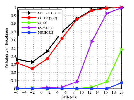
In Fig. 5, we can notice that in terms of PR the suggested MS-KAI-CG-FB outperforms the ordinary CG algorithm equipped with forward-backward spatial smoothing, denoted as CG-FB, the ordinary CG algorithm, MUSIC and ESPRIT in most of the considered range of SNR values.
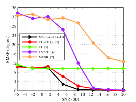
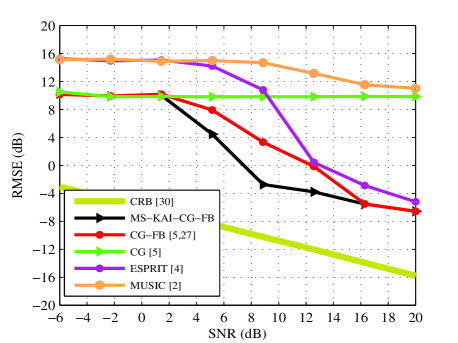
In Fig. 6, we can see that in terms of RMSE the proposed MS-KAI-CG-FB provides the best performance in the range dB. It can also be seen that in the ranges dB and dB its performance is similar to the best. This performance can be better noticed in Fig. 7, which shows the RMSE of all curves which form the preceding graphic and the square root of the deterministic CRB [100], all of them in terms of dB.
VII Conclusions
We have developed the MS-KAI-CG algorithm and its version equipped with forward-backward spatial smoothing termed MS-KAI-CG-FB algorithm. Both approaches exploit the knowledge of signals and the structure of the data covariance matrix, which are acquired on line and used to subtract unwanted terms, thereby improving the performance of existing CG-based DoA estimation algorithms. In scenarios composed of two uncorrelated closely-spaced sources and a sufficient number of snapshots, the MS-KAI-CG algorithm has shown its superiority in terms of probability of resolution and RMSE over existing algorithms, including the original CG, in the low and medium levels of SNR, i.e., in the range . In scenarios in which the uncorrelated signals previously considered were replaced with strongly correlated signals, the comparisons of MS-KAI-CG-FB algorithm with existing algorithms, including the original CG and its version equipped with forward-backward spatial smoothing (CG-FB), have shown a superior accuracy to the MS-KAI-CG-FB algorithm in the following significant ranges: in , for probability of resolution; and , for RMSE. Based on the significant improvements pointed out, we can consider that MS-KAI-CG and MS-KAI-CG-FB for dealing with correlated sources have excellent potential for applications with significant data records in large-scale sensor array systems for wireless communications, radar and other applications with large sensor arrays.
References
- [1] Van Trees, H. L.: ’Optimum Array Processing’, (Wiley,New York, 2002).
- [2] H. Ruan and R. C. de Lamare, “Robust Adaptive Beamforming Using a Low-Complexity Shrinkage-Based Mismatch Estimation Algorithm,” IEEE Sig. Proc. Letters., Vol. 21, No. 1, pp 60-64, 2014.
- [3] A. Elnashar, “Efficient implementation of robust adaptive beamforming based on worst-case performance optimization,” IET Signal Process., Vol. 2, No. 4, pp. 381-393, Dec 2008.
- [4] J. Zhuang and A. Manikas, “Interference cancellation beamforming robust to pointing errors,” IET Signal Process., Vol. 7, No. 2, pp. 120-127, April 2013.
- [5] L. Wang and R. C. de Lamare, “Constrained adaptive filtering algorithms based on conjugate gradient techniques for beamforming,” IET Signal Process., Vol. 4, No. 6, pp. 686-697, Feb 2010.
- [6] H. Ruan and R. C. de Lamare, ”Robust Adaptive Beamforming Based on Low-Rank and Cross-Correlation Techniques,” in IEEE Transactions on Signal Processing, vol. 64, no. 15, pp. 3919-3932, 1 Aug.1, 2016.
- [7] H. Ruan and R. C. de Lamare, “Low-Complexity Robust Adaptive Beamforming Based on Shrinkage and Cross-Correlation,” 19th International ITG Workshop on Smart Antennas, pp 1-5, March 2015.
- [8] L. L. Scharf and D. W. Tufts, “Rank reduction for modeling stationary signals,” IEEE Transactions on Acoustics, Speech and Signal Processing, vol. ASSP-35, pp. 350-355, March 1987.
- [9] A. M. Haimovich and Y. Bar-Ness, “An eigenanalysis interference canceler,” IEEE Trans. on Signal Processing, vol. 39, pp. 76-84, Jan. 1991.
- [10] D. A. Pados and S. N. Batalama ”Joint space-time auxiliary vector filtering for DS/CDMA systems with antenna arrays” IEEE Transactions on Communications, vol. 47, no. 9, pp. 1406 - 1415, 1999.
- [11] J. S. Goldstein, I. S. Reed and L. L. Scharf ”A multistage representation of the Wiener filter based on orthogonal projections” IEEE Transactions on Information Theory, vol. 44, no. 7, 1998.
- [12] Y. Hua, M. Nikpour and P. Stoica, ”Optimal reduced rank estimation and filtering,” IEEE Transactions on Signal Processing, pp. 457-469, Vol. 49, No. 3, March 2001.
- [13] M. L. Honig and J. S. Goldstein, “Adaptive reduced-rank interference suppression based on the multistage Wiener filter,” IEEE Transactions on Communications, vol. 50, no. 6, June 2002.
- [14] E. L. Santos and M. D. Zoltowski, “On Low Rank MVDR Beamforming using the Conjugate Gradient Algorithm”, Proc. IEEE International Conference on Acoustics, Speech and Signal Processing, 2004.
- [15] Q. Haoli and S.N. Batalama, “Data record-based criteria for the selection of an auxiliary vector estimator of the MMSE/MVDR filter”, IEEE Transactions on Communications, vol. 51, no. 10, Oct. 2003, pp. 1700 - 1708.
- [16] R. C. de Lamare and R. Sampaio-Neto, “Reduced-Rank Adaptive Filtering Based on Joint Iterative Optimization of Adaptive Filters”, IEEE Signal Processing Letters, Vol. 14, no. 12, December 2007.
- [17] Z. Xu and M.K. Tsatsanis, “Blind adaptive algorithms for minimum variance CDMA receivers,” IEEE Trans. Communications, vol. 49, No. 1, January 2001.
- [18] R. C. de Lamare and R. Sampaio-Neto, “Low-Complexity Variable Step-Size Mechanisms for Stochastic Gradient Algorithms in Minimum Variance CDMA Receivers”, IEEE Trans. Signal Processing, vol. 54, pp. 2302 - 2317, June 2006.
- [19] C. Xu, G. Feng and K. S. Kwak, “A Modified Constrained Constant Modulus Approach to Blind Adaptive Multiuser Detection,” IEEE Trans. Communications, vol. 49, No. 9, 2001.
- [20] Z. Xu and P. Liu, “Code-Constrained Blind Detection of CDMA Signals in Multipath Channels,” IEEE Sig. Proc. Letters, vol. 9, No. 12, December 2002.
- [21] R. C. de Lamare and R. Sampaio Neto, ”Blind Adaptive Code-Constrained Constant Modulus Algorithms for CDMA Interference Suppression in Multipath Channels”, IEEE Communications Letters, vol 9. no. 4, April, 2005.
- [22] L. Landau, R. C. de Lamare and M. Haardt, “Robust adaptive beamforming algorithms using the constrained constant modulus criterion,” IET Signal Processing, vol.8, no.5, pp.447-457, July 2014.
- [23] R. C. de Lamare, “Adaptive Reduced-Rank LCMV Beamforming Algorithms Based on Joint Iterative Optimisation of Filters”, Electronics Letters, vol. 44, no. 9, 2008.
- [24] R. C. de Lamare and R. Sampaio-Neto, “Adaptive Reduced-Rank Processing Based on Joint and Iterative Interpolation, Decimation and Filtering”, IEEE Transactions on Signal Processing, vol. 57, no. 7, July 2009, pp. 2503 - 2514.
- [25] R. C. de Lamare and Raimundo Sampaio-Neto, “Reduced-rank Interference Suppression for DS-CDMA based on Interpolated FIR Filters”, IEEE Communications Letters, vol. 9, no. 3, March 2005.
- [26] R. C. de Lamare and R. Sampaio-Neto, “Adaptive Reduced-Rank MMSE Filtering with Interpolated FIR Filters and Adaptive Interpolators”, IEEE Signal Processing Letters, vol. 12, no. 3, March, 2005.
- [27] R. C. de Lamare and R. Sampaio-Neto, “Adaptive Interference Suppression for DS-CDMA Systems based on Interpolated FIR Filters with Adaptive Interpolators in Multipath Channels”, IEEE Trans. Vehicular Technology, Vol. 56, no. 6, September 2007.
- [28] R. C. de Lamare, “Adaptive Reduced-Rank LCMV Beamforming Algorithms Based on Joint Iterative Optimisation of Filters,” Electronics Letters, 2008.
- [29] R. C. de Lamare and R. Sampaio-Neto, “Reduced-rank adaptive filtering based on joint iterative optimization of adaptive filters”, IEEE Signal Process. Lett., vol. 14, no. 12, pp. 980-983, Dec. 2007.
- [30] R. C. de Lamare, M. Haardt, and R. Sampaio-Neto, “Blind Adaptive Constrained Reduced-Rank Parameter Estimation based on Constant Modulus Design for CDMA Interference Suppression”, IEEE Transactions on Signal Processing, June 2008.
- [31] M. Yukawa, R. C. de Lamare and R. Sampaio-Neto, “Efficient Acoustic Echo Cancellation With Reduced-Rank Adaptive Filtering Based on Selective Decimation and Adaptive Interpolation,” IEEE Transactions on Audio, Speech, and Language Processing, vol.16, no. 4, pp. 696-710, May 2008.
- [32] R. C. de Lamare and R. Sampaio-Neto, “Reduced-rank space-time adaptive interference suppression with joint iterative least squares algorithms for spread-spectrum systems,” IEEE Trans. Vehi. Technol., vol. 59, no. 3, pp. 1217-1228, Mar. 2010.
- [33] R. C. de Lamare and R. Sampaio-Neto, “Adaptive reduced-rank equalization algorithms based on alternating optimization design techniques for MIMO systems,” IEEE Trans. Vehi. Technol., vol. 60, no. 6, pp. 2482-2494, Jul. 2011.
- [34] R. C. de Lamare, L. Wang, and R. Fa, “Adaptive reduced-rank LCMV beamforming algorithms based on joint iterative optimization of filters: Design and analysis,” Signal Processing, vol. 90, no. 2, pp. 640-652, Feb. 2010.
- [35] R. Fa, R. C. de Lamare, and L. Wang, “Reduced-Rank STAP Schemes for Airborne Radar Based on Switched Joint Interpolation, Decimation and Filtering Algorithm,” IEEE Transactions on Signal Processing, vol.58, no.8, Aug. 2010, pp.4182-4194.
- [36] L. Wang and R. C. de Lamare, ”Low-Complexity Adaptive Step Size Constrained Constant Modulus SG Algorithms for Blind Adaptive Beamforming”, Signal Processing, vol. 89, no. 12, December 2009, pp. 2503-2513.
- [37] L. Wang and R. C. de Lamare, “Adaptive Constrained Constant Modulus Algorithm Based on Auxiliary Vector Filtering for Beamforming,” IEEE Transactions on Signal Processing, vol. 58, no. 10, pp. 5408-5413, Oct. 2010.
- [38] L. Wang, R. C. de Lamare, M. Yukawa, ”Adaptive Reduced-Rank Constrained Constant Modulus Algorithms Based on Joint Iterative Optimization of Filters for Beamforming,” IEEE Transactions on Signal Processing, vol.58, no.6, June 2010, pp.2983-2997.
- [39] L. Wang, R. C. de Lamare and M. Yukawa, “Adaptive reduced-rank constrained constant modulus algorithms based on joint iterative optimization of filters for beamforming”, IEEE Transactions on Signal Processing, vol.58, no. 6, pp. 2983-2997, June 2010.
- [40] L. Wang and R. C. de Lamare, “Adaptive constrained constant modulus algorithm based on auxiliary vector filtering for beamforming”, IEEE Transactions on Signal Processing, vol. 58, no. 10, pp. 5408-5413, October 2010.
- [41] R. Fa and R. C. de Lamare, “Reduced-Rank STAP Algorithms using Joint Iterative Optimization of Filters,” IEEE Transactions on Aerospace and Electronic Systems, vol.47, no.3, pp.1668-1684, July 2011.
- [42] Z. Yang, R. C. de Lamare and X. Li, “L1-Regularized STAP Algorithms With a Generalized Sidelobe Canceler Architecture for Airborne Radar,” IEEE Transactions on Signal Processing, vol.60, no.2, pp.674-686, Feb. 2012.
- [43] Z. Yang, R. C. de Lamare and X. Li, “Sparsity-aware space–time adaptive processing algorithms with L1-norm regularisation for airborne radar”, IET signal processing, vol. 6, no. 5, pp. 413-423, 2012.
- [44] Neto, F.G.A.; Nascimento, V.H.; Zakharov, Y.V.; de Lamare, R.C., ”Adaptive re-weighting homotopy for sparse beamforming,” in Signal Processing Conference (EUSIPCO), 2014 Proceedings of the 22nd European , vol., no., pp.1287-1291, 1-5 Sept. 2014
- [45] Almeida Neto, F.G.; de Lamare, R.C.; Nascimento, V.H.; Zakharov, Y.V.,“Adaptive reweighting homotopy algorithms applied to beamforming,” IEEE Transactions on Aerospace and Electronic Systems, vol.51, no.3, pp.1902-1915, July 2015.
- [46] L. Wang, R. C. de Lamare and M. Haardt, “Direction finding algorithms based on joint iterative subspace optimization,” IEEE Transactions on Aerospace and Electronic Systems, vol.50, no.4, pp.2541-2553, October 2014.
- [47] S. D. Somasundaram, N. H. Parsons, P. Li and R. C. de Lamare, “Reduced-dimension robust capon beamforming using Krylov-subspace techniques,” IEEE Transactions on Aerospace and Electronic Systems, vol.51, no.1, pp.270-289, January 2015.
- [48] S. Xu and R.C de Lamare, , Distributed conjugate gradient strategies for distributed estimation over sensor networks, Sensor Signal Processing for Defense SSPD, September 2012.
- [49] S. Xu, R. C. de Lamare, H. V. Poor, “Distributed Estimation Over Sensor Networks Based on Distributed Conjugate Gradient Strategies”, IET Signal Processing, 2016 (to appear).
- [50] S. Xu, R. C. de Lamare and H. V. Poor, Distributed Compressed Estimation Based on Compressive Sensing, IEEE Signal Processing letters, vol. 22, no. 9, September 2014.
- [51] S. Xu, R. C. de Lamare and H. V. Poor, “Distributed reduced-rank estimation based on joint iterative optimization in sensor networks,” in Proceedings of the 22nd European Signal Processing Conference (EUSIPCO), pp.2360-2364, 1-5, Sept. 2014
- [52] S. Xu, R. C. de Lamare and H. V. Poor, “Adaptive link selection strategies for distributed estimation in diffusion wireless networks,” in Proc. IEEE International Conference onAcoustics, Speech and Signal Processing (ICASSP), , vol., no., pp.5402-5405, 26-31 May 2013.
- [53] S. Xu, R. C. de Lamare and H. V. Poor, “Dynamic topology adaptation for distributed estimation in smart grids,” in Computational Advances in Multi-Sensor Adaptive Processing (CAMSAP), 2013 IEEE 5th International Workshop on , vol., no., pp.420-423, 15-18 Dec. 2013.
- [54] S. Xu, R. C. de Lamare and H. V. Poor, “Adaptive Link Selection Algorithms for Distributed Estimation”, EURASIP Journal on Advances in Signal Processing, 2015.
- [55] N. Song, R. C. de Lamare, M. Haardt, and M. Wolf, “Adaptive Widely Linear Reduced-Rank Interference Suppression based on the Multi-Stage Wiener Filter,” IEEE Transactions on Signal Processing, vol. 60, no. 8, 2012.
- [56] N. Song, W. U. Alokozai, R. C. de Lamare and M. Haardt, “Adaptive Widely Linear Reduced-Rank Beamforming Based on Joint Iterative Optimization,” IEEE Signal Processing Letters, vol.21, no.3, pp. 265-269, March 2014.
- [57] R.C. de Lamare, R. Sampaio-Neto and M. Haardt, ”Blind Adaptive Constrained Constant-Modulus Reduced-Rank Interference Suppression Algorithms Based on Interpolation and Switched Decimation,” IEEE Trans. on Signal Processing, vol.59, no.2, pp.681-695, Feb. 2011.
- [58] Y. Cai, R. C. de Lamare, “Adaptive Linear Minimum BER Reduced-Rank Interference Suppression Algorithms Based on Joint and Iterative Optimization of Filters,” IEEE Communications Letters, vol.17, no.4, pp.633-636, April 2013.
- [59] R. C. de Lamare and R. Sampaio-Neto, “Sparsity-Aware Adaptive Algorithms Based on Alternating Optimization and Shrinkage,” IEEE Signal Processing Letters, vol.21, no.2, pp.225,229, Feb. 2014.
- [60] R. C. de Lamare, “Massive MIMO Systems: Signal Processing Challenges and Future Trends”, Radio Science Bulletin, December 2013.
- [61] W. Zhang, H. Ren, C. Pan, M. Chen, R. C. de Lamare, B. Du and J. Dai, “Large-Scale Antenna Systems With UL/DL Hardware Mismatch: Achievable Rates Analysis and Calibration”, IEEE Trans. Commun., vol.63, no.4, pp. 1216-1229, April 2015.
- [62] R. C. De Lamare and R. Sampaio-Neto, ”Minimum Mean-Squared Error Iterative Successive Parallel Arbitrated Decision Feedback Detectors for DS-CDMA Systems,” in IEEE Transactions on Communications, vol. 56, no. 5, pp. 778-789, May 2008.
- [63] R. C. de Lamare, ”Adaptive and Iterative Multi-Branch MMSE Decision Feedback Detection Algorithms for Multi-Antenna Systems,” in IEEE Transactions on Wireless Communications, vol. 12, no. 10, pp. 5294-5308, October 2013.
- [64] Y. Cai, R. C. de Lamare, B. Champagne, B. Qin and M. Zhao, ”Adaptive Reduced-Rank Receive Processing Based on Minimum Symbol-Error-Rate Criterion for Large-Scale Multiple-Antenna Systems,” in IEEE Transactions on Communications, vol. 63, no. 11, pp. 4185-4201, Nov. 2015.
- [65] A. G. D. Uchoa, C. T. Healy and R. C. de Lamare, ”Iterative Detection and Decoding Algorithms for MIMO Systems in Block-Fading Channels Using LDPC Codes,” in IEEE Transactions on Vehicular Technology, vol. 65, no. 4, pp. 2735-2741, April 2016.
- [66] P. Li and R. C. de Lamare, ”Distributed Iterative Detection With Reduced Message Passing for Networked MIMO Cellular Systems,” in IEEE Transactions on Vehicular Technology, vol. 63, no. 6, pp. 2947-2954, July 2014.
- [67] K. Zu, R. C. de Lamare and M. Haardt, ”Multi-Branch Tomlinson-Harashima Precoding Design for MU-MIMO Systems: Theory and Algorithms,” in IEEE Transactions on Communications, vol. 62, no. 3, pp. 939-951, March 2014.
- [68] W. Zhang et al., ”Widely Linear Precoding for Large-Scale MIMO with IQI: Algorithms and Performance Analysis,” in IEEE Transactions on Wireless Communications, vol. 16, no. 5, pp. 3298-3312, May 2017.
- [69] J. Gu, R. C. de Lamare and M. Huemer, ”Buffer-Aided Physical-Layer Network Coding With Optimal Linear Code Designs for Cooperative Networks,” in IEEE Transactions on Communications, vol. 66, no. 6, pp. 2560-2575, June 2018.
- [70] Schmidt, R.: ’Multiple emitter location and signal parameter estimation’, IEEE Trans on Antennas and Propagation, 34, (3), pp 276-280, 1986.
- [71] Barabell, A. J.: ’Improving the resolution performance of eigenstructure-based direction-finding algorithms’, Proc. Int. Conf. on Acoustic Speech and Signal Processing ICASSP, Boston, pp. 336-339, 1983.
- [72] Roy, R. and Kailath, T: ’Estimation of signal parameters via rotational invariance techniques’, IEEE Trans. Acoust., Speech and Signal Processing, 37, pp 984-995, 1989.
- [73] L. Wang and R. C. DeLamare, ”Low-Complexity Constrained Adaptive Reduced-Rank Beamforming Algorithms,” in IEEE Transactions on Aerospace and Electronic Systems, vol. 49, no. 4, pp. 2114-2128, October 2013.
- [74] S. D. Somasundaram, N. H. Parsons, P. Li and R. C. de Lamare, ”Reduced-dimension robust capon beamforming using Krylov-subspace techniques,” in IEEE Transactions on Aerospace and Electronic Systems, vol. 51, no. 1, pp. 270-289, January 2015.
- [75] Semira, H., Belkacemi, Marcos, S.: ’High-resolution source localization algorithm based on the Conjugate Gradient’, EURASIP Journal on Advances in Signal Processing, 2007.
- [76] Steinwandt, J.,Lamare, R., Haardt, M.: ’Beamspace direction finding based on the conjugate gradient and the auxiliary vector filtering algorithms’, Signal Processing, 93, (4), pp. 641-651, 2013.
- [77] Wang, L., Lamare, R., Haardt, M.: ’Direction finding algorithms based on joint iterative subspace optimization’, IEEE Transactions on Aerospace and Electronic Systems, 50, (4), pp. 2541-2553, 2014.
- [78] Qiu, L., Lamare, R., Zhao, M.: ’Reduced-Rank DOA Estimation Algorithms Based on Alternating Low-Rank Decomposition’, IEEE Signal Processing Letters23, (5), pp. 565-569, May 2016.
- [79] Pal, P., Vaidyanathan, P.P.: ’A Novel Approach to Array Processing With Enhanced Degrees of Freedom’,IEEE Transactions on Signal Processing, 58, (8), pp. 4167-4181, 2010.
- [80] Pal, P., Vaidyanathan, P.P.:’Sparse sensing with co-prime samplers and arrays’, IEEE Transactions on Signal Processing, 59, (2), pp. 573-586, 2011.
- [81] Zhou, C., Gu, Y., Zhang, Y.D., Shi, Z., Jin, T., Wu,X.:’Compressive sensing-based coprime array direction-of-arrival estimation’, IET Communications, 11, (11), pp. 1719-1724, 2017.
- [82] Shi, Z., Zhou, C., Gu, Y., Goodman, N.A., Qu, F.:’Source Estimation using Coprime Array: A Sparse Reconstruction Perspective’, IEEE Sensors Journal, 17, (3), pp. 755-765, 2017.
- [83] Pinto, S., Lamare, R: ’Two-Step Knowledge-aided Iterative ESPRIT Algorithm’, Proc. IEEE Twenty First ITG Workshop on Smart Antennas, Berlin, Germany, pp. 1-5, March 2017.
- [84] Pinto, S., Lamare, R.: ’Multi-Step Knowledge-Aided Iterative ESPRIT for Direction Finding’, Proc. IEEE 22nd International Conference on Digital Signal Processing, London, UK, pp. 1-5, August 2017.
- [85] Pinto, S., Lamare, R: ’Multi-Step Knowledge-Aided Iterative ESPRIT: Design and Analysis’, IEEE Transactions on Aerospace and Electronic Systems, (early access), pp 1-1, 2018.
- [86] Pinto, S., Lamare, R.: ’ Multi-Step Knowledge-Aided Iterative Conjugate Gradient for Direction Finding’, Proc. IEEE 22nd ITG Workshop on Smart Antennas, Bochum, Germany, 2018.
- [87] Shaghaghi, M., Vorobyov, S.: ’ Iterative root-MUSIC algorithm for DOA estimation’, Proc. IEEE 5th International Workshop on Computational Advances in Multisensor Adaptive Processing, 2013.
- [88] Shaghaghi, M., Vorobyov, S.: ’Subspace leakage analysis and improved DOA estimation with small sample size’, IEEE Trans. Signal Processing,63, (12), pp 3251-3265, 2015.
- [89] Pinto, S., Lamare, R.: ’Knowledge-Aided Parameter Estimation Based on Conjugate Gradient Algorithms’, 35th Brazilian Communications and Signal Processing Symposium, Sao Pedro, SP, Brazil, pp.1-5, 2017.
- [90] Steinwandt, J.,Lamare, R., Haardt, M.: ’Knowledge-aided direction finding based on Unitary ESPRIT’, Proc IEEE 45th Asilomar Conference on Signals, Systems and Computers, pp. 613-617, 2011.
- [91] Stoica, P., Zhu, X., Guerci, J.: ’On using a priori knowledge in space-time adaptive processing’, IEEE Transactions on Signal Processing, pp. 2598-2602, 2008.
- [92] Liberti Jr,J., Rappaport,T.: ’Smart antennas for Wireless Communications: IS-95 and Third Generation CDMA Applications’, Prentice Hall, 1999.
- [93] Schell,S, Gardner, W.:’High Resolution Direction Finding’, Handbook of Statistics, Elsevier, 1993.
- [94] Rissanen,J.: ’Modeling by the Shortest Data Description’, Automatica, 14, pp 465-471, 1978.
- [95] Stoica, P., Nehorai, A.: ’Performance study of conditional and unconditional direction-of-arrival estimation’, IEEE Trans. Acoust., Speech, Signal Processing, 38, (10), pp. 1783-1795, 1990,
- [96] Stoica, P., Gershman, A.: ’Maximum-likelihood DOA estimation by data-supported grid search’, IEEE Signal Processing Letters, pp. 273-275, 1999.
- [97] Pillai, S., Kwon B.: ’Forward/Backward spatial smoothing techniques for coherent signal identification’, IEEE Trans. Acoustics, Speech, and Signal Processing, pp. 8-15, 1989.
- [98] Thakre, A., Haardt, M., Giridhar, K: ’Single Snapshot Spatial Smoothing with Improved Effective Array Aperture’, IEEE Signal Processing Letters, 6, 2009.
- [99] Steinwandt, J., Lamare, R. C., Haardt, M.: “Beamspace direction finding based on the conjugate gradient algorithm”, 2011, International ITG Workshop on Smart Antennas, pp.1-5, Feb. 2011, included in IEEE Xplore in April 2011.
- [100] Stoica, P., Nehorai, A.: ’MUSIC, maximum Likelihood, and Cramér-Rao Bound’, IEEE Transactions on Acoustics, Speech and Signal Processing, pp. 720- 741, 1989.
- [101] Grover, R., Pados, D., Medley, M.: ’Subspace direction finding with an auxiliary-vector basis’, IEEE Transactions on Signal Processing, pp.758-763, 2007.
- [102] Golub, G. , van Loan, C.: ”Matrix Computations”, Johns Hopkins University Press, 3rd edition, 1996.
- [103] Y. Cai, R. C. d. Lamare and R. Fa, ”Switched Interleaving Techniques with Limited Feedback for Interference Mitigation in DS-CDMA Systems,” in IEEE Transactions on Communications, vol. 59, no. 7, pp. 1946-1956, July 2011.
- [104] Y. Cai, R. C. de Lamare and D. Le Ruyet, ”Transmit Processing Techniques Based on Switched Interleaving and Limited Feedback for Interference Mitigation in Multiantenna MC-CDMA Systems,” in IEEE Transactions on Vehicular Technology, vol. 60, no. 4, pp. 1559-1570, May 2011.
- [105] K. Zu and R. C. d. Lamare, ”Low-Complexity Lattice Reduction-Aided Regularized Block Diagonalization for MU-MIMO Systems,” in IEEE Communications Letters, vol. 16, no. 6, pp. 925-928, June 2012.
- [106] K. Zu, R. C. de Lamare and M. Haardt, ”Generalized Design of Low-Complexity Block Diagonalization Type Precoding Algorithms for Multiuser MIMO Systems,” in IEEE Transactions on Communications, vol. 61, no. 10, pp. 4232-4242, October 2013.
- [107] W. Zhang et al., ”Widely Linear Precoding for Large-Scale MIMO with IQI: Algorithms and Performance Analysis,” in IEEE Transactions on Wireless Communications, vol. 16, no. 5, pp. 3298-3312, May 2017.
- [108] K. Zu, R. C. de Lamare and M. Haardt, ”Multi-Branch Tomlinson-Harashima Precoding Design for MU-MIMO Systems: Theory and Algorithms,” in IEEE Transactions on Communications, vol. 62, no. 3, pp. 939-951, March 2014.
- [109] L. Zhang, Y. Cai, R. C. de Lamare and M. Zhao, ”Robust Multibranch Tomlinson–Harashima Precoding Design in Amplify-and-Forward MIMO Relay Systems,” in IEEE Transactions on Communications, vol. 62, no. 10, pp. 3476-3490, Oct. 2014.
- [110] L. T. N. Landau and R. C. de Lamare, ”Branch-and-Bound Precoding for Multiuser MIMO Systems With 1-Bit Quantization,” in IEEE Wireless Communications Letters, vol. 6, no. 6, pp. 770-773, Dec. 2017.
- [111] R. C. de Lamare and R. Sampaio-Neto, ”Adaptive Reduced-Rank Processing Based on Joint and Iterative Interpolation, Decimation, and Filtering,” in IEEE Transactions on Signal Processing, vol. 57, no. 7, pp. 2503-2514, July 2009.
- [112] R. C. de Lamare and R. Sampaio-Neto, ”Reduced-Rank Adaptive Filtering Based on Joint Iterative Optimization of Adaptive Filters,” in IEEE Signal Processing Letters, vol. 14, no. 12, pp. 980-983, Dec. 2007.
- [113] R. C. de Lamare and R. Sampaio-Neto, ”Adaptive Reduced-Rank Processing Based on Joint and Iterative Interpolation, Decimation, and Filtering,” in IEEE Transactions on Signal Processing, vol. 57, no. 7, pp. 2503-2514, July 2009.
- [114] R. C. de Lamare and P. S. R. Diniz, ”Set-Membership Adaptive Algorithms Based on Time-Varying Error Bounds for CDMA Interference Suppression,” in IEEE Transactions on Vehicular Technology, vol. 58, no. 2, pp. 644-654, Feb. 2009.
- [115] R. C. De Lamare and R. Sampaio-Neto, ”Blind adaptive MIMO receivers for space-time block-coded DS-CDMA systems in multipath channels using the constant modulus criterion,” in IEEE Transactions on Communications, vol. 58, no. 1, pp. 21-27, January 2010.
- [116] Y. Cai, R. C. de Lamare, B. Champagne, B. Qin and M. Zhao, ”Adaptive Reduced-Rank Receive Processing Based on Minimum Symbol-Error-Rate Criterion for Large-Scale Multiple-Antenna Systems,” in IEEE Transactions on Communications, vol. 63, no. 11, pp. 4185-4201, Nov. 2015.
- [117] R. C. de Lamare and R. Sampaio-Neto, ”Adaptive MBER decision feedback multiuser receivers in frequency selective fading channels,” in IEEE Communications Letters, vol. 7, no. 2, pp. 73-75, Feb. 2003.
- [118] R. C. De Lamare and R. Sampaio-Neto, ”Minimum Mean-Squared Error Iterative Successive Parallel Arbitrated Decision Feedback Detectors for DS-CDMA Systems,” in IEEE Transactions on Communications, vol. 56, no. 5, pp. 778-789, May 2008.
- [119] P. Li, R. C. de Lamare and R. Fa, ”Multiple Feedback Successive Interference Cancellation Detection for Multiuser MIMO Systems,” in IEEE Transactions on Wireless Communications, vol. 10, no. 8, pp. 2434-2439, August 2011.
- [120] P. Li and R. C. De Lamare, ”Adaptive Decision-Feedback Detection With Constellation Constraints for MIMO Systems,” in IEEE Transactions on Vehicular Technology, vol. 61, no. 2, pp. 853-859, Feb. 2012.
- [121] P. Li and R. C. de Lamare, ”Distributed Iterative Detection With Reduced Message Passing for Networked MIMO Cellular Systems”, IEEE Transactions on Vehicular Technology, vol. 63, no. 6, pp. 2947-2954, 2014.
- [122] P. Clarke and R. C. de Lamare, ”Transmit Diversity and Relay Selection Algorithms for Multirelay Cooperative MIMO Systems,” in IEEE Transactions on Vehicular Technology, vol. 61, no. 3, pp. 1084-1098, March 2012.
- [123] T. Peng, R. C. de Lamare and A. Schmeink, ”Adaptive Distributed Space-Time Coding Based on Adjustable Code Matrices for Cooperative MIMO Relaying Systems,” in IEEE Transactions on Communications, vol. 61, no. 7, pp. 2692-2703, July 2013.
- [124] T. Peng and R. C. de Lamare, ”Adaptive Buffer-Aided Distributed Space-Time Coding for Cooperative Wireless Networks,” in IEEE Transactions on Communications, vol. 64, no. 5, pp. 1888-1900, May 2016.
- [125] A. G. D. Uchoa, C. T. Healy and R. C. de Lamare, ”Iterative Detection and Decoding Algorithms for MIMO Systems in Block-Fading Channels Using LDPC Codes,” in IEEE Transactions on Vehicular Technology, vol. 65, no. 4, pp. 2735-2741, April 2016.
- [126] Z. Shao, R. C. de Lamare and L. T. N. Landau, ”Iterative Detection and Decoding for Large-Scale Multiple-Antenna Systems With 1-Bit ADCs,” in IEEE Wireless Communications Letters, vol. 7, no. 3, pp. 476-479, June 2018.
- [127] J. Gu, R. C. de Lamare and M. Huemer, ”Buffer-Aided Physical-Layer Network Coding With Optimal Linear Code Designs for Cooperative Networks,” in IEEE Transactions on Communications, vol. 66, no. 6, pp. 2560-2575, June 2018.
- [128] A. G. D. Uchoa, C. Healy, R. C. de Lamare and R. D. Souza, ”Design of LDPC Codes Based on Progressive Edge Growth Techniques for Block Fading Channels,” in IEEE Communications Letters, vol. 15, no. 11, pp. 1221-1223, November 2011.
- [129] C. T. Healy and R. C. de Lamare, ”Design of LDPC Codes Based on Multipath EMD Strategies for Progressive Edge Growth,” in IEEE Transactions on Communications, vol. 64, no. 8, pp. 3208-3219, Aug. 2016.