Spectral analysis of the extremely hot DA white dwarf PG 0948+534

Abstract

There is a striking paucity of hydrogen-rich (DA) white dwarfs (WDs) relative to their hydrogen-deficient (non-DA) counterparts at the very hot end of the WD cooling sequence. The three hottest known DAs (surface gravity $\log\,g$ $\geq$ 7.0) have effective temperatures around $T\mathrm{{}_{eff}}$ = 140 000 K, followed by only five objects in the range 104 000 – 120 000 K. They are by far outnumbered by forty non-DAs with $T\mathrm{{}_{eff}}$ = 100 000 – 250 000 K, giving a DA/non-DA ratio of 0.2. In contrast, this ratio is the inverse of that for the cooler WDs. One reason for this discrepancy could be uncertainties in the temperature determination of hot DAs using Balmer-line spectroscopy. Recent investigations involving metal-ionization balances in ultraviolet (UV) spectra indeed showed that the temperatures of some DAs were underestimated, but the paucity of extremely hot DAs prevailed. Here we present the results of a UV spectral analysis of one of the three hottest DAs, PG 0948+534. We find that its temperature was strongly overestimated by recent Balmer line analyses. We correct it downward to 105 000 $\pm$ 5000 K, aggravating the hot-DA paucity. The Balmer-line problem encountered previously is not resolved by our non-LTE line-blanketed model atmospheres. We speculate that it might be related to the possible presence of a magnetosphere. This is supported by the V-band variability that shows a period of $P=3.45$ d (amplitude 0.19 mag), which we interpret as the star’s rotation period. The metal abundances in PG 0948+534 are affected by atomic diffusion and we conclude that the onset of diffusion in hot DAs occurs when they cool below $T\mathrm{{}_{eff}}$ $\approx 105\,000$ K. We discuss the possibility that the paucity of very hot DAs is a consequence of their fast evolutionary rate.

1 Introduction

The number of hydrogen-rich (spectral types DA and DAO) white dwarfs (WDs) with effective temperatures ($T\mathrm{{}_{eff}}$) of 100 000 K or higher and $\log\,g$ $\geq$ 7.0 is very small. Only eight such objects are currently known (Tab. 1). This paucity of extremely hot H-rich WDs is in stark contrast to the much larger number of forty hydrogen-poor (non-DA) WDs with $T\mathrm{{}_{eff}}$ $\geq$ 100 000 K and $\log\,g$ $\geq$ 7, that are 14 helium-rich (DO) WDs and 26 He- and C-rich (PG1159) stars (see Werner & Herwig (2006) and Werner et al., in prep.). Hence, the DA/non-DA ratio at the hottest end of the WD cooling sequence is 0.2, while for the cooler WDs, that ratio is near five (Bergeron et al. 2011). In Fig. 1 we depict the location of all known WDs with $T\mathrm{{}_{eff}}$ $\geq$ 100 000 K and $\log\,g$ $\geq$ 7.0 in the $g$ – $T\mathrm{{}_{eff}}$  diagram.

Table 1: Currently known hydrogen-rich WDs with $T\mathrm{{}_{eff}}$ $\geq$ 100 000 K and $\log\,g$ $\geq$ 7.0. All results were obtained with NLTE models. For the three hottest WDs, Balmer line fits were performed, while for the others metal lines were exploited to constrain $T\mathrm{{}_{eff}}$ . For the star analyzed in the present paper, PG 0948+534, we quote the latest literature result (for earlier results and the values derived here see Table 2).

Name	WD name	Type	$T\mathrm{{}_{eff}}$ /K	$\log\,g$	Technique	Reference
EGB 1	WD0103$+$732	DAO	147 000 $\pm$ 25 000	7.34 $\pm$ 0.31	NLTE Balmer	Napiwotzki (1999)
WeDe 1	WD0556$+$106	DA	141 000 $\pm$ 19 000	7.53 $\pm$ 0.32	NLTE Balmer	Napiwotzki (1999)
PG 0948+534	WD0948$+$534	DA	141 000 $\pm$ 12 000	7.46 $\pm$ 0.18	NLTE Balmer	Preval & Barstow (2017); see Table 2
Longmore 1	–	DAO	120 000 $\pm$ 10 000	7.00 $\pm$ 0.30	NLTE metals	Ziegler (2012)
Abell 31	WD0851$+$090	DAO	114 000 $\pm$ 10 000	7.40 $\pm$ 0.30	NLTE metals	Ziegler (2012)
Abell 7	WD0500$-$156	DAO	109 000 $\pm$ 10 000	7.00 $\pm$ 0.30	NLTE metals	Ziegler (2012)
EGB 6	WD0950$+$139	DAO	105 000 $\pm$   5 000	7.40 $\pm$ 0.40	NLTE metals	Werner et al. (2018b)
NGC 3587	WD1111$+$552	DAO	104 000 $\pm$ 10 000	7.00 $\pm$ 0.60	NLTE metals	Ziegler (2012)

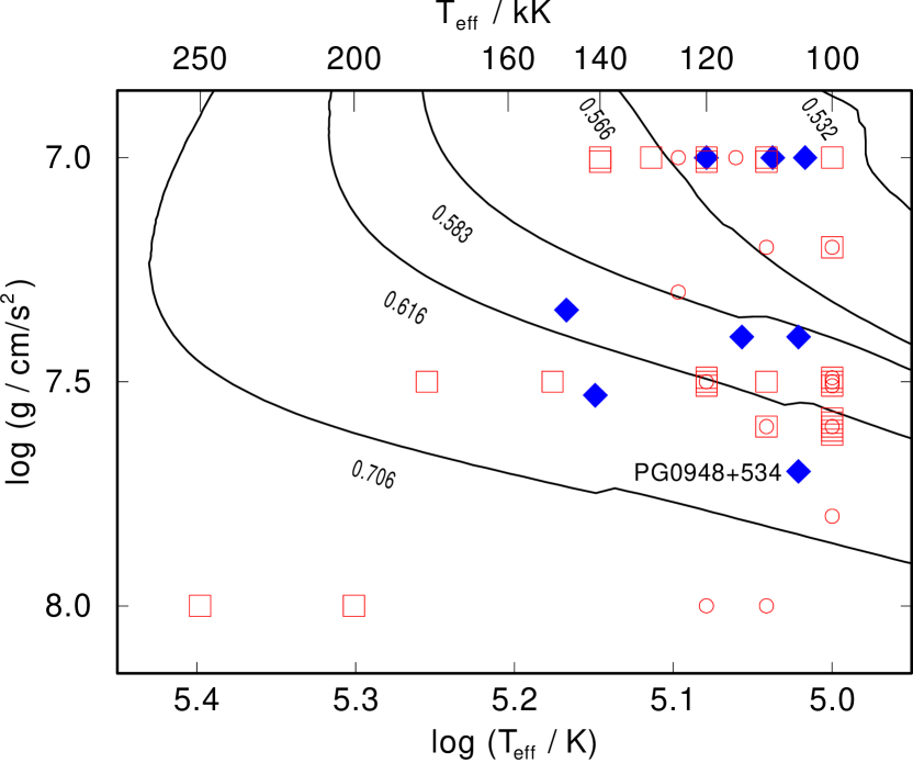
Figure 1: Presently known DA (blue rhombs) and non-DA (red symbols) WDs with $T\mathrm{{}_{eff}}$ $\geq$ 100 000 K and $\log\,g$ $\geq$ 7.0. Red squares and circles denote PG1159 stars and DO WDs, respectively. The position of PG 0948+534 is shown according to the result of this work. Black lines are evolutionary tracks of post-AGB remnants with masses as labeled (in $M_{\odot}$, from Miller Bertolami 2016, metallicity $Z=0.01$).

This phenomenon has been discussed in the literature since decades, when a lack of very hot DAs in the Palomar-Green (PG) survey (Green et al. 1986) was reported (Liebert 1986). For example, the central star of the planetary nebula WeDe 1 (= WDHS 1) was initially regarded as the only hydrogen-rich WD with a “PG1159-like” $T\mathrm{{}_{eff}}$  and gravity (about 140 000 K and $\log\,g$ = 7.0) by Liebert et al. (1994). The authors emphasized, however, that the parameters of the H-rich WDs remain uncertain because of unknown element abundances and the so-called Balmer-line problem. It was speculated that the improvement of model atmospheres might show that the number of DAs and DAOs increases substantially. The basic problem is the large uncertainty when the analyses solely rely on optical spectra. In the case of DAs, only the Balmer lines are available and in addition He ii $\lambda$4686 in the DAOs. A further complication is the appearance of the Balmer-line problem for many of the hottest DAs (Napiwotzki 1992), meaning that for a particular object different temperatures follow from fits to different Balmer line series members. This problem is still not fully understood. To some extent it is due to the neglect of metal opacities in the models (Werner 1996), but it was found in many cases that the problem does not disappear even if sophisticated metal-line blanketed models are used (e.g., Werner et al. 2018b).

While initially LTE model atmospheres were used for spectral analyses, the subsequent employment of non-LTE models was more appropriate considering the high temperatures. But the lack of a more precise temperature indicator, the ionization balance of any species, remained and left analyses based on Balmer lines with high uncertainties. In the case of non-DAs, lines from highly ionized C, N, O, and Ne are seen in the optical spectra of many objects, so the situation is better for these stars and analysis results are more reliable. The only possibility to improve the precision of parameter estimations of the hottest DA(O)s is ultraviolet (UV) spectroscopy. Here, lines from many species in different ionization stages are usually detected.

Analyses of hot DA(O)s employing UV spectroscopy showed that a number of the hottest objects are in fact even hotter than previously thought. For example, the temperatures of some of the WDs analyzed by Napiwotzki (1999) using Balmer lines, were shown to be above 100 000 K when UV spectroscopy was employed. One example is the central star of Abell 31, for which $T\mathrm{{}_{eff}}$ = 84 700 K was derived from the Balmer lines, while Ziegler et al. (2012) found 114 000 K from a detailed analysis of metals lines in the UV. In this sense, the temperatures of the objects listed in Table 1 that were determined from Balmer line spectroscopy alone must be regarded uncertain. Interestingly, this is the case of the three hottest ones, which have temperatures around 140 000 K. These are the just mentioned central star of WeDe 1, the central star of EGB 1, and PG 0948+534. From these three stars, UV spectroscopy is only available for PG 0948+534  therefore we are assessing it in the present study.

Table 2: Previous determinations of effective temperature and gravity for PG 0948+534 as derived from Lyman and Balmer line fits and result of this work. The two different sets of values from Preval & Barstow (2017) using Lyman lines were obtained employing different line-broadening tables. The metal abundances used in the NLTE model structures computed by Barstow et al. (2003), Gianninas et al. (2010) and Preval & Barstow (2017) were chosen by an approximative estimate (see text and in Table 3 lines “B03 model”, “G10 model”, “P17 model”, respectively). The entry “(+metals)” set in brackets means that metals were included in the model atmosphere, but metal lines were not used to constrain $T\mathrm{{}_{eff}}$  and $\log\,g$ .

$T\mathrm{{}_{eff}}$ /K	$\log\,g$	Technique	Reference
126 300	7.27	LTE, Balmer	Liebert & Bergeron (1995)
110 000 $\pm$ 2 500	7.58 $\pm$ 0.06	NLTE (+metals), Balmer	Barstow et al. (2003)
130 370 $\pm$ 6 603	7.26 $\pm$ 0.12	NLTE, Balmer	Liebert et al. (2005)
139 500	7.56	NLTE (+metals), Balmer	Gianninas et al. (2010, 2011)
138 000 $\pm$ 7 000	8.43 $\pm$ 0.10	NLTE (+metals), Lyman	Preval & Barstow (2017); line broadening of Lemke (1997)
140 000 $\pm$ 8 000	8.60 $\pm$ 0.10	NLTE (+metals), Lyman	Preval & Barstow (2017); line broadening of Tremblay & Bergeron (2009)
141 000 $\pm$ 12 000	7.46 $\pm$ 0.18	NLTE (+metals), Balmer	Preval & Barstow (2017)
105 000 $\pm$ 5 000	7.70 $\pm$ 0.20	NLTE+metals, metal lines, Lyman	This work

Table 3: Assumed and derived metal abundances in previous studies compared to the result of the present work (last line). Abundances given as number ratio relative to hydrogen. B03: Barstow et al. (2003); “model” denotes the abundances assumed for the model calculation and “synspec” denotes abundances derived by fitting of metal lines without considering back-reaction on population numbers and atmospheric structure (no fits to lines from C, N, O, and Si could be achieved). P17: Preval & Barstow (2017); same procedure, but considering more species. G10: Gianninas et al. (2010); assumed abundances.

	C	N	O	Si	P	S	Ar	Fe	Ni
B03 model	$4.0\cdot 10^{-7}$	$1.6\cdot 10^{-7}$	$9.6\cdot 10^{-7}$	$3.0\cdot 10^{-7}$	$-$	$-$	$-$	$1.0\cdot 10^{-5}$	$5.0\cdot 10^{-7}$
synspec	$-$	$-$	$-$	$-$	$-$	$-$	$-$	$1.9\cdot 10^{-6}$	$1.2\cdot 10^{-7}$
P17 model	$1.0\cdot 10^{-6}$	$1.0\cdot 10^{-6}$	$1.0\cdot 10^{-5}$	$1.0\cdot 10^{-6}$	$1.0\cdot 10^{-7}$	$1.0\cdot 10^{-7}$	$3.0\cdot 10^{-5}$	$1.0\cdot 10^{-6}$	$1.0\cdot 10^{-6}$
synspec	$2.8\cdot 10^{-6}$	$9.1\cdot 10^{-7}$	$1.5\cdot 10^{-5}$	$1.5\cdot 10^{-5}$	$9.2\cdot 10^{-8}$	$1.4\cdot 10^{-6}$	$1.1\cdot 10^{-6}$	$1.2\cdot 10^{-5}$	$3.8\cdot 10^{-6}$
G10 model	$2.5\cdot 10^{-4}$	$6.0\cdot 10^{-5}$	$4.6\cdot 10^{-4}$	$-$	$-$	$-$	$-$	$-$	$-$
This work	$<2.5\cdot 10^{-6}$	$2.2\cdot 10^{-7}$	$3.2\cdot 10^{-8}$	$7.2\cdot 10^{-6}$	$1.6\cdot 10^{-7}$	$1.6\cdot 10^{-6}$	$9.1\cdot 10^{-7}$	$5.4\cdot 10^{-5}$	$6.9\cdot 10^{-6}$

With the advent of the Far Ultraviolet Spectroscopic Explorer (FUSE), it became possible to use the Lyman line series beyond Ly$\alpha$ as diagnostics for a large number of DA(O)s. However, it turned out that particularly for the hottest stars, systematic differences between the results derived from Lyman and Balmer line analyses appeared (Barstow et al. 2001). This discrepancy is still not understood (Preval et al. 2015). One example is the DA of the present study for which parameter estimates widely differ as we will describe later.

We report here on our analysis of UV spectra of PG 0948+534 taken with FUSE and the Hubble Space Telescope (HST) in order to find out whether this WD is indeed one of the three hottest DAs known or if it is significantly cooler. In the latter case, the paucity of hot hydrogen-rich WDs relative to the non-DAs would become even more evident.

We begin with an overview of previous work on this WD in the following Section. Then we describe our spectral analysis in Sect. 2. In Sect. 4 we report on the variability of the star and we conclude with a summary and discussion of our results in Sect. 5.

2 Previous studies of PG 0948+534

Numerous attempts were made over more than the past two decades to determine effective temperature and gravity of PG 0948+534 (Table 2). To understand the significant scatter in the derived results, it is necessary but also instructive to report in some detail the used analysis techniques and atmosphere models. Initially, the star was identified as an extremely hot DA ($T\mathrm{{}_{eff}}$ = 126 000 K) by Liebert & Bergeron (1995), fitting the Balmer lines with pure-hydrogen LTE models. In a systematic analysis of WDs from the PG survey (Green et al. 1986) it was found that PG 0948+534 is by far the hottest DA in that sample ($T\mathrm{{}_{eff}}$ = 130 370 K, Liebert et al. 2005), and the only DA together with PG 0950+139, the central star of the planetary nebula EGB 6 ($T\mathrm{{}_{eff}}$ = 105 000 K, Liebert et al. 2005; Werner et al. 2018b), that exceed $T\mathrm{{}_{eff}}$ = 100 000 K. It was also emphasized that this was the first DA exhibiting the Balmer line problem, a phenomenon up to then restricted to DAO WDs.

The first spectral analysis using NLTE models was performed by Barstow et al. (2003). To account for the effects of metal opacities on the atmospheric structure and the Balmer lines (Werner 1996), they included, as a first approximation, several species in the calculations (C, N, O, Si, Fe, Ni), assuming abundances equal to that derived for another hot DA (G191-B2B), see Table 3; line “B03 model”. As a result, the Balmer line fit arrived at a lower temperature of 110 000 K (and $\log\,g$ = 7.58). Keeping fixed these atmospheric values, Fe and Ni abundances were derived from UV spectra (Table 3; line “B03 synspec”) by varying the original abundance estimates in the formal solution for the radiation transfer, only (i.e., disregarding back-reaction on population numbers and atmospheric structure), but that procedure failed to achieve a fit to lines of C, N, O, and Si in the UV spectra. A later attempt with chemically stratified models failed, too (Dickinson et al. 2012a).

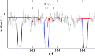
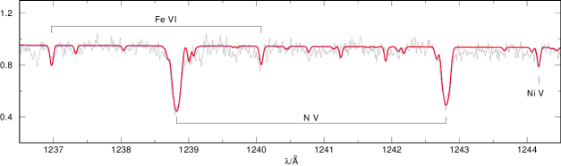
Figure 2: Spectral regions with a N iv multiplet (left) and the N v resonance doublet (right). N iv lines in the model (red) are not detectable in the observation (grey), thus, $T\mathrm{{}_{eff}}$ $>100\,000$ K. The blue graph is our model attenuated by simulated ISM Lyman lines.

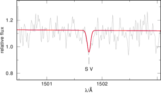
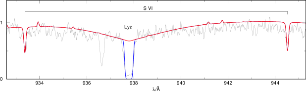
Figure 3: Fits to S v $\lambda$1502 (left) and the S vi resonance doublet (right).

In a subsequent NLTE analysis Gianninas et al. (2010) derived a significantly higher temperature of almost 140 000 K (and $\log\,g$ = 7.56) from Balmer lines. The only difference in their model grid compared to the previous NLTE study was the assumption of other metal abundances (solar values, including the species C, N, and O; see Table 3; line “G10 model”). The most recent assessment of the Balmer-line profiles of PG 0948+534 was presented by Preval & Barstow (2017). Their analysis procedure, using a model with 110 000 K, $\log\,g$ = 7.58, was the same like in Barstow et al. (2003), but additional species were included (P, S, Ar). The abundances derived in an approximate way (again, assuming an initial estimate, line “B17 model” in Table 3, and just varying abundances in the formal solutions to find the values given in line “B17 synspec” in Table 3), were then used to compute a new model grid to find improved values for $T\mathrm{{}_{eff}}$  and $\log\,g$  from the Balmer and Lyman lines. From the Balmer lines they found a much higher temperature (141 000 K and $\log\,g$ = 7.46) compared to their previous study (110 000 K). Most puzzling however, was the result of their fit to the Lyman lines in the FUSE spectrum with this model grid. While the same high effective temperature was derived like for the Balmer lines ($\approx$ 140 000 K), an extremely large value for the surface gravity was determined ($\log\,g$ = 8.43 – 8.60, depending in detail on the used line-broadening tables). This is in strong contrast to the gravity estimates from their and all previous Balmer line fits, which gave values of $\log\,g$  in the narrow range 7.26 – 7.56.

To summarize the findings of the previous studies, rather conflicting results for $T\mathrm{{}_{eff}}$  (110 000 – 141 000 K) and $\log\,g$  (7.26 – 8.60) were derived. For the present paper, we set out to determine these parameters more precisely by employing UV metal lines as sensitive temperature indicators and to determine metal abundances in order to compute a self-consistent atmosphere structure.

3 Spectral analysis

3.1 UV observations

We used archival spectra of PG 0948+534 taken with FUSE and HST. Three observations were performed with FUSE (Data IDs A0341501000, –2000, and –3000) in 2007 and 2008 with a total exposure time of 16 218 s. However, in the first and second of these observations, data of two channels are missing while in the third observation all four channels are complete. We co-added the available spectra. The useful range is 910–1180 Å. The star was also observed with the Space Telescope Imaging Spectrograph (STIS) aboard HST during four consecutive orbits on April 20, 2000, using grating E140M at central wavelength 1425 Å (Datasets O59P05010, –20, –30, –40). The co-added spectrum has a total exposure time of 11 958 s and was retrieved from the StarCAT catalogue (Ayres 2010). Its useful wavelength range is 1150–1710 Å.

Considering the optical variability of the star with an amplitude of $\Delta V=0.19$ mag and a period of 3.45 d (Sect. 4), we inspected the UV flux for variability. The four sub-exposures of the STIS observation were taken within a time span of just 6% of the variability period. The flux levels of the three FUSE exposures do not differ by more than 10 %. Also, there is no significant difference in the flux levels of the co-added FUSE spectrum and the HST spectrum in the wavelength region where they overlap. A comparison of the HST spectrum with a low-resolution spectrum taken with the International Ultraviolet Explorer (image SWP14328) in 1981 also shows no obvious difference.

In all respective figures displayed in this paper, the photospheric lines were shifted to rest wavelengths. The photospheric lines in the HST spectrum are blueshifted by $v_{\rm phot}$ = $-10$ km/s, as indicated by, e.g., the N v resonance doublet, O v $\lambda$1371, S v $\lambda$1502, and several Fe vi lines. Dickinson et al. (2012b) derived, from the same HST spectrum, a significantly higher value of $-17$ km/s. This can be traced back to the fact that they assigned the strong C iv resonance doublet (at this redshift) to the photosphere, but we will show below that it is in fact dominated by an interstellar absorption component. The photospheric lines in the FUSE spectrum are blueshifted by $v_{\rm phot}\approx-25$ km/s, but we note that the absolute wavelength calibration of the FUSE data is not as reliable as that of STIS. To account for the FUSE spectral resolving power (R = 20 000), the model spectra were convolved with a 0.05 Å (FWHM) Gaussian. In some cases, the observations were slightly smoothed (with up to 0.03 Å Gaussians). The model spectra fitted to the STIS observations were convolved with Gaussians to account for the resolution (R = 38 000), i.e., their FWHM is ranging from 0.030 to 0.045 Å over the spectral window 1150–1710 Å.

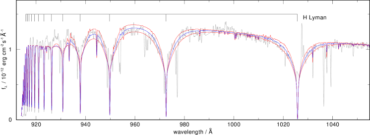
Figure 4: Observed Lyman lines from Ly$\beta$ to the series limit, compared to three models with different surface gravity, $\log\,g$ = 7.7 (blue graph) and $\pm$0.5 dex (red graphs). $T\mathrm{{}_{eff}}$  and element abundances according to final model (Table 4). Model fluxes are normalized to the observed continuum at 1050 Å, reddened ($E(B-V)=0.02$), and attenuated by ISM interstellar neutral H absorption ($n_{\rm HI}=2.4\times 10^{19}$ cm^-2), the latter affecting the innermost Ly line cores, only. For clarity, observation and models are smoothed by 0.2 Å Gaussians.

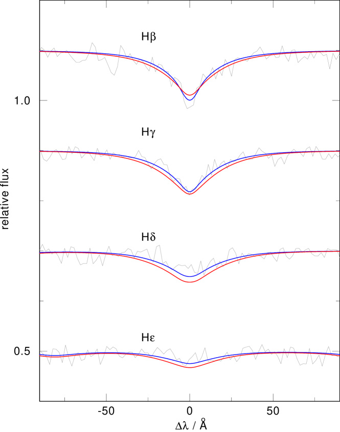
Figure 5: Observed Balmer lines compared to our final model (blue graph) and a model with the same parameters but without metals (red).

3.2 Model atmospheres

We used the Tübingen Model-Atmosphere Package (TMAP) to compute non-LTE, plane-parallel, line-blanketed atmosphere models in radiative and hydrostatic equilibrium (Werner & Dreizler 1999; Werner et al. 2003; Werner et al. 2012). The models include H, He, C, N, O, Si, P, S, Fe, and Ni. The employed model atoms were described in detail by Werner et al. (2018a). In addition, we performed line formation iterations (i.e., keeping the atmospheric structure fixed) for argon using the model atom presented in Werner et al. (2015). Since the treatment of Lyman line broadening was a topic in previous works, we mention that we used the broadening tables of Tremblay & Bergeron (2009).

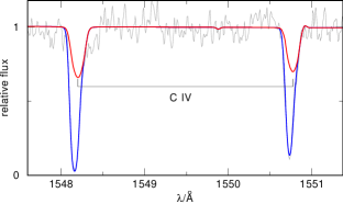
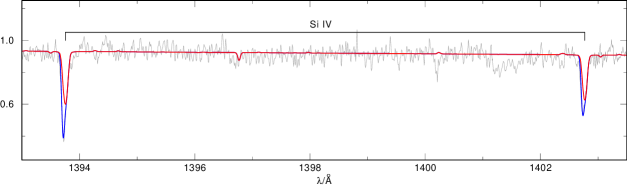
Figure 6: Left panel: The observed C iv resonance doublet is dominated by ISM absorption (fitted by the blue graph). The weaker photospheric contribution is indicated by the model (red graph) computed with the upper abundance limit for C derived from the absence of subordinate C iv lines. Right panel: The computed Si iv resonance doublet has an ISM (blue graph) and a photospheric contribution (red graph).

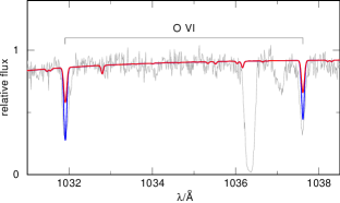
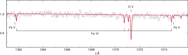
Figure 7: Fits to the O vi resonance doublet (left) and O v $\lambda$1371 (right). The O vi doublet is not matched by the model and could be dominated by ISM contribution (blue graph).

3.3 Effective temperature and surface gravity

To find a model that best fits the metal lines in the UV spectra, we followed a manual, iterative procedure to improve the fits by computing a sequence of models successively, changing effective temperature and abundances. At the outset, we kept fixed the surface gravity to $\log\,g$ = 7.7, a value guided by the Balmer-line fits in the literature (Table 2). To constrain $T\mathrm{{}_{eff}}$ , the relative strengths of lines from different ionization stages of a given chemical element were used. Most useful is the fact, that PG 0948+534 displays lines from four ionization stages of iron, namely Fe v-viii. This immediately constrains the temperature to the narrow range of 100 000 – 110 000 K. Cooler and hotter models do not exhibit the lines detected from Fe viii and Fe v, respectively. Ionization balances from other elements are in accordance with this temperature range. While the N v resonance doublet depends weakly on $T\mathrm{{}_{eff}}$ , the N iv lines are very sensitive. The non-detection of the N iv multiplet near 923 Å (Fig. 2) requires $T\mathrm{{}_{eff}}$ $>$100 000 K. On the other hand, sulfur gives a strong upper limit. At 110 000 K the S v 1502 Å line (Fig. 3) is becoming too weak, while at 105 000 K it fits well, together with the S vi resonance doublet. We conclude $T\mathrm{{}_{eff}}$ = 105 000$\pm$5000 K. The only serious problem is posed by the O vi resonance doublet, which is much too weak in the model, when O v $\lambda$1371 fits well. This mismatch between the O v and O vi lines cannot be mitigated with models of different temperature within reasonable limits. We will discuss below, that an ISM contribution to O vi could be an explanation for this discrepancy.

Having found the best fitting model in this way, we then considered deviations from the assumed value of $\log\,g$ = 7.7. We computed models with different gravity, keeping fixed all other model parameters and compared the resulting Lyman lines with the observations, with the exception of Ly$\alpha$, which is dominated by ISM absorption over the entire profile. The higher Lyman series members are dominated by ISM contribution in the innermost cores only.

In Fig. 4 we compare model profiles of Ly$\beta$ and higher series members with the observation. We show our final model ($T\mathrm{{}_{eff}}$ = 105 000 K, $\log\,g$ = 7.7) together with two models with gravity increased and decreased by 0.5 dex. Obviously, the line profiles do not depend strongly on gravity, so that we must accept a relatively large error of $\pm 0.4$ dex. As we shall see below (Sect. 3.6), the parallax of PG 0948+534 favors $\log\,g$ = 7.6, so that we finally adopt a smaller error of $\pm 0.2$ dex. It can be seen that the continuum flux level at the highest series members at wavelengths shorter than about 930 Å is not quite matched by our models. In fact, it is almost identical in all three models, which means that level dissolution has essentially eliminated photospheric line opacities (the narrow line features are interstellar absorptions). The flux below this wavelength threshold is therefore unaffected by line opacities and thus determined by the effective temperature. So a slight increase in $T\mathrm{{}_{eff}}$  to 110 000 K leads to a better continuum flux fit, but this is within our error range for the temperature. Note that the flux cut-off at 912 Å is entirely due to interstellar neutral H absorption, which is included in the models shown in Fig. 4 ($n_{\rm HI}=2.4\times 10^{19}$ cm^-2, Sect. 3.4.4).

We also assessed the question why Preval & Barstow (2017) could arrive at extraordinary high gravities of around $\log\,g$ = 8.6 in their Lyman line fitting. We computed a model with that gravity and $T\mathrm{{}_{eff}}$ = 140 000 K, i.e., the parameters they derived, and compared it to our 105 000/7.7 model. It turns out that the effect of an increase in $T\mathrm{{}_{eff}}$  on the Lyman line profiles can to a large extent be compensated by an increase in $\log\,g$ . Both models show differences in the wings of Ly$\beta$ to Ly$\delta$ that are smaller than a few percent, only. So, even small errors in the flux calibration can lead to large errors in the determination of $T\mathrm{{}_{eff}}$  and $\log\,g$ . We also note that we have included interstellar reddening ($E(B-V)=0.02$, Sect. 3.4.4) in the model fluxes displayed in Fig. 4, which does affect the continuum shape and must therefore be considered in flux fitting across this wide wavelength range. We will show below (Sect. 3.6), that the parallax of PG 0948+534 independently excludes high gravities.

In the final model calculations, helium is included with an abundance value identical to the upper limit determined from the absence of He ii $\lambda$1640, i.e., He $=3\times 10^{-4}$ (by mass).

We compared an optical spectrum of PG 0948+534 covering H$\beta$ and higher Balmer series members with our final model and noticed that the Balmer-line problem is still present; the H$\beta$ line core of the model is not deep enough (Fig. 5). The influence of C, N, and O on the model structure is relatively weak because of the strongly subsolar abundances of these species (see next Section).

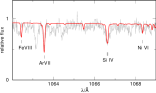
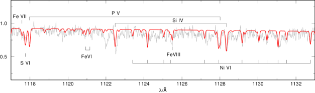
Figure 8: Left: Lines from Si iv, Ar vii, Fe viii, and Ni vi. Right: Lines from Si iv, P v, S vi, Fe vi-viii, and Ni vi.

3.4 Element abundance determination

Element abundances were derived from line profile fits as indicated in the following. All quoted abundance values are given in mass fractions.

3.4.1 Carbon, nitrogen, and oxygen

Carbon lines cannot be identified. An upper abundance limit of C = $3\times 10^{-5}$ is obtained from the absence of the C iv $\lambda$1168.8/1169.0 3d–4f doublet in the HST spectrum. The FUSE spectrum at this position is contaminated by a He i $\lambda$1168.67 airglow line (second order from $\lambda$584.33). This C limit is in accordance with the absence of the C iv 1107.6/1107.9 3p–4d doublet. The weak absorption features visible in the FUSE spectrum at these wavelengths are due to Ni vi lines. Looking at the observed C iv resonance doublet (Fig. 6) reveals that it must be dominated by interstellar absorption (blueshifted by 8 km/s relative to the photospheric component). The computed photospheric line is much weaker. The C upper abundance limit is compatible with the observed line profile. A significantly higher abundance would be detectable in the red wings of the interstellar line profiles.

The only detectable nitrogen lines are the N v resonance doublet (Fig. 2). There is no indication for a blueshifted ISM component as in the case of the C iv resonance doublet. As mentioned above, the absence of the N iv multiplet near 923 Å (Fig. 2) imposes a lower limit for $T\mathrm{{}_{eff}}$ .

O v $\lambda$1371 and the O vi $\lambda\lambda$1032/1038 resonance doublet are very prominent lines (Fig. 7). The oxygen abundance is derived by fitting the O v line because no interstellar contribution is expected. With this abundance, the O vi doublet is much too weak. The observed O v line is weaker than the O vi doublet. In order to reduce the relative O v/O vi line strength in the model to the observed extent, $T\mathrm{{}_{eff}}$  would need to be as high as 140 000 K. Another option would be a significantly lower $T\mathrm{{}_{eff}}$  of about 90 000 K, when the temperature becomes too low to keep the O v line strong, whereas the O vi resonance doublet remains more prominent. But these temperature extremes are excluded by ionization balances of other metals (N, S, Fe, Ni), see above.

A possible explanation for this discrepancy could be a dominant ISM contribution to the O vi doublet, similar to the case of the C iv doublet. The FUSE spectral resolution is not sufficient to detect such a component with relative blueshift of 8 km/s. Assuming an interstellar column density of $n_{\rm OVI}=5.0\times 10^{13}$ cm^-2 gives a good fit to the observed line strengths. Similar $n_{\rm OVI}$ values were found towards a number of WDs in the sample investigated by Barstow et al. (2010) to probe the O vi content in the local ISM.

3.4.2 Silicon, phosphorus, sulfur, and argon

The silicon abundance was found from two Si iv doublets, namely the 3p–3d lines at 1122.5/1128.3 Å (Fig. 8), and the 3s–3p resonance doublet at 1393.8/1402.8 Å (Fig. 6). Similar to C iv, the photospheric Si iv resonance doublet is blended by an interstellar component with a relative blueshift of 9 km/s. Another Si iv line, the 3d–4f transition at 1066.6 Å, is detected (Fig. 8).

The phosphorus abundance was found from fitting the P v $\lambda\lambda$1118/1128 resonance doublet (Fig. 8).

A singlet line from S v at 1502 Å (Fig. 3, left panel) and the S vi $\lambda\lambda$933/945 3s–3p resonance doublet (Fig. 3, right panel) were used to infer the sulfur abundance. Two weaker S vi lines are seen at 1000.5 Å (4d–5f) and at 1117.8 Å (4f–7g, Fig. 8).

We have previously announced the detection of the strong Ar vii $\lambda$1063.55 line, which is the counterpart of the above-mentioned $\lambda$1502 line in the isoelectronic S v (Werner et al. 2007). The argon abundance we derived here (Ar = $3.6\times 10^{-5}$) is in agreement with our earlier work ($7.9\times 10^{-5}$) within error limits, though not identical because our present model atmosphere is slightly cooler, and includes more species and has more realistic metal abundances.

3.4.3 Iron and nickel

We detected a large number of lines from Fe vi, some from Fe vii, and a few from Fe viii and Fe v, see examples in Figs. 2, 7, and 8. The iron ionization balance is very temperature sensitive (see above) and we obtained a good fit to the lines of all four observed ionization stages at a slightly oversolar iron abundance.

We identified a large number of nickel lines from ionization stages Ni v (Fig. 2) and Ni vi (Fig. 8). Like for iron, we derived a slightly oversolar nickel abundance.

Table 4: Results of spectroscopic analysis of PG 0948+534 and derived parameters. Abundances in number ratios relative to H (column 2), in mass fractions (column 3), and logarithmic mass fractions relative to solar value (column 4; solar abundances from Asplund et al. 2009). Error limits for metal abundances are $\pm 0.5$ dex.

$T\mathrm{{}_{eff}}$ / K	$105\,000\pm 5000$
$\log$($g$/cm/s2)	$7.7\pm 0.2$
$E(B-V)$	$0.02\pm 0.01$
$n_{\rm H}$/cm-2	$(2.4\pm 0.2)\times 10^{19}$
$M\,/\,M_{\odot}$	$0.66^{+0.06}_{-0.06}$
$d$ / pc	$361^{+93}_{-74}$
abundances	$N_{i}/N_{H}$	$X_{i}$	[$X_{i}$]
H	1	0.996	0.13
He	$<7.6\times 10^{-5}$	$<3.0\times 10^{-4}$	$<-2.92$
C	$<2.5\times 10^{-6}$	$<3.0\times 10^{-5}$	$<-1.86$
N	$2.2\times 10^{-7}$	$3.0\times 10^{-6}$	$-2.31$
O	$3.2\times 10^{-8}$	$5.0\times 10^{-7}$	$-4.03$
Si	$7.2\times 10^{-6}$	$2.0\times 10^{-4}$	$-0.52$
P	$1.6\times 10^{-7}$	$5.0\times 10^{-6}$	$-0.02$
S	$1.6\times 10^{-6}$	$5.0\times 10^{-5}$	$-0.81$
Ar	$9.1\times 10^{-7}$	$3.6\times 10^{-5}$	$-0.31$
Fe	$5.4\times 10^{-5}$	$3.0\times 10^{-3}$	0.42
Ni	$6.9\times 10^{-6}$	$4.0\times 10^{-4}$	0.74

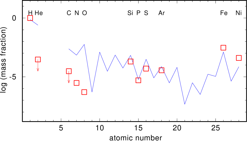
Figure 9: Measured element abundances in PG 0948+534 (red squares) in comparison to solar abundances (blue line).

3.4.4 Reddening and ISM neutral hydrogen column density

From a comparison of the overall UV flux distribution of PG 0948+534 with our final model we found a reddening of $E(B-V)=0.02\pm 0.01$, in agreement with the 3D dust map of Green et al. (2018), which gives $E(B-V)=0.02\pm 0.02$ at the Gaia distance (Sect. 3.6) of the star. The Ly$\alpha$ line profile is dominated by ISM absorption. We derived an interstellar neutral hydrogen column density of $n_{\rm HI}=(2.4\pm 0.2)\times 10^{19}$ cm^-2.

3.5 Summary of spectral analysis

The results of our analysis are summarized in Table 4 and in Fig. 9. We determined $T\mathrm{{}_{eff}}$ = 105 000 $\pm$ 5000 K and $\log\,g$ = 7.7 $\pm$ 0.2. The temperature is lower than that of all previous analyses, which were in the range 110 000 – 141 000 K. The gravity is in accordance with previous studies (7.27 – 7.58) when the extreme values of 8.43 – 8.60 found from Lyman line fits (Preval & Barstow 2017) are excluded.

The abundances of He, C, N, and O are strongly subsolar by about 2 – 4 dex (upper limits for C and He). Slight underabundances of Si, P, S, and Ar were found (0.02 – 0.8 dex) and slight overabundances of Fe and Ni (0.42 and 0.74 dex). The main difference to the earlier work by Preval & Barstow (2017) is our much lower value of the oxygen abundance (reduced by 2.7 dex), because we concluded that the O vi resonance doublet is probably dominated by an ISM contribution. We also found that the carbon abundance determined by Preval & Barstow (2017) must be regarded as an upper limit, because we showed that the C iv resonance doublet is dominated by an ISM contribution.

3.6 WD mass and distance

The stellar mass is estimated from the comparison of the determined atmospheric parameters $T\mathrm{{}_{eff}}$  and $\log\,g$  with evolutionary tracks by Miller Bertolami (2016). We found $M\,/\,M_{\odot}=0.66^{+0.06}_{-0.06}$. The errors are dominated by the uncertainty in $g$.

The spectroscopic distance $d$ was found by comparing the dereddened visual magnitude $V_{0}$ with the respective model atmosphere flux, resulting in the relation

$$d{\rm[pc]}=7.11\times 10^{4}\sqrt{H_{\nu}\cdot M\cdot 10^{0.4V_{0}-\log g}}\ ,$$

where $H_{\nu}=1.54\times 10^{-3}$ erg cm^-2s^-1Hz^-1 is the Eddington flux of the model at 5400 Å, and $M$ is the stellar mass in $M_{\odot}$. For our WD we have $V=15.32$ mag (Drake et al. 2009), but note that this is an average value since it is variable by about $\pm 0.1$ mag (see Sect. 4). From $E(B-V)=0.02$ we derived the visual extinction using the standard relation $A_{V}=3.1\times E(B-V)=0.062$, hence $V_{0}=15.26$. We found $d=361^{+93}_{-74}$ pc and the main error source is our uncertainty in the gravity ($\log\,g$ = $7.7\pm 0.2$). The distance to the WD given in the Gaia Data Release 2 ($318\pm 7$ pc) is in good agreement. A perfect match would require $\log\,g$ = 7.6, while on the other hand the unrealistically high value of $\log\,g$ = 8.6 (Preval & Barstow 2017) would give a spectroscopic distance of only 140 pc.

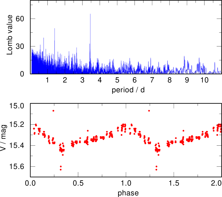
Figure 10: Periodogram (top) and light curve (bottom) of PG 0948+534.

4 Variability

We obtained the V-band light curve of PG 0948+534 from the 2nd data release of the Catalina Sky Survey and calculated a Lomb-Scargle periodogram. We found a period of $P=3.45$ d (false-alarm probability $<10^{-28}$) and an amplitude of 0.19 mag. Periodogram and phase folded light curve are shown in Fig. 10. The light curve was classified as of RS CVn type (Drake et al. 2014). That are usually close binaries with late-type components, $P$ being the orbital period. We suspect that in the case of PG 0948+534 a weak magnetic field causes a spotted surface (plus possible effects of a magnetosphere, see discussion below) and $P$ is the WD rotation period.

5 Results and conclusion

We have analyzed the UV spectrum of the hot DA PG 0948+534. We found that its effective temperature is significantly lower than recent estimates from Balmer- and Lyman-line fits. This corroborates earlier results from detailed UV spectroscopy that the temperature estimates particularly from Balmer-line fits of the hottest hydrogen-rich WDs must be regarded as rather uncertain. While Ziegler (2012) found that $T\mathrm{{}_{eff}}$  was often underestimated, we encountered here a case where $T\mathrm{{}_{eff}}$  was significantly overestimated, so there is no clear systematic trend. PG 0948+534 was thought to be among the three by far hottest DA WDs (with $\log\,g$ $\geq$ 7.0) having $T\mathrm{{}_{eff}}$ $\approx$ 140 000 K. It could be that the two others are also cooler, because their temperature was also derived from Balmer lines. UV spectra are unavailable for them. The fact that WeDe 1 is not a DAO but a DA argues against an effective temperature as high as 141 000 K (see below). Our result aggravates the problem that many more non-DA WDs than DAs are known at the very hot end of the WD cooling sequence.

The large scatter of results from Balmer-line fits for PG 0948+534 in different works shows that systematic errors in the data reduction and fitting techniques are severe in the case of the hottest DAs. The same holds for the Lyman lines where effects of gravity and temperature are difficult to disentangle. An important step forward would be a systematic analysis of available UV spectra of all hot DAs in the manner presented here.

A further complication of optical spectral analyses is introduced by the Balmer-line problem, which is encountered with the majority of hot DAs (Tremblay et al. 2011) and in PG 0948+534 as well (Bergeron et al. 1994). It is not entirely removed by using metal-line blanketed models, as we have seen in our analysis but also, e.g., in a recent analysis of the DAO EGB 6, which has similar atmospheric parameters (Werner et al. 2018b). Obviously, there is a remaining deficit in the model atmospheres. It has been speculated that the Balmer-line problem might be an indication for the presence of a magnetosphere as recently revealed for a DO WD exhibiting ultrahigh-ionization lines (Reindl et al. 2019). If true, then an early speculation by Napiwotzki (1992) about the presence of a weak photospheric magnetic field affecting the Balmer lines would turn out to be partly correct, albeit in a somewhat different sense. A relation of the Balmer-line problem in PG 0948+534 with the possible presence of a magnetosphere is corroborated by the fact that the WD exhibits a periodic variability ($P=3.45$ d, V-band amplitude 0.19 mag). This is similar to what is detected at the above-mentioned DO, which has a shorter rotation period (0.24 d) but a similar V-band amplitude (0.17 mag). Starspots originating from a magnetic field and/or geometrical effects of the optically thick, circumstellar magnetosphere are thought to cause the variability (Reindl et al. 2019). Phase-resolved UV spectroscopy could shed more light on the origin of the observed optical variability.

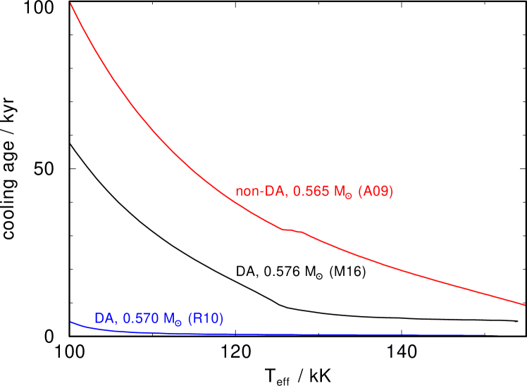
Figure 11: Cooling age of WD models with similar mass (see labels) down to $T\mathrm{{}_{eff}}$ = 100 000 K. The non-DA model is a very-late thermal pulse track from Althaus et al. (2009) (A09). The two DA models are from Miller Bertolami (2016) (M16) and from Renedo et al. (2010) (R10).

Let us look at the cooling times of DA and non-DA WDs in the high-$T\mathrm{{}_{eff}}$  regime considered in this paper. In Fig. 11 we compare the cooling age of three WD models which have very similar mass, namely one non-DA and two DA models. The DAs cool faster than the non-DA, but it is surprising that the two DA models have so different cooling rates. One possible explanation is that the rate could depend on the thermal-pulse phase when the model has left the Asymptotic Giant Branch (Miller-Bertolami, priv. comm.; but note that this is only relevant in the very earliest cooling phases). Given this uncertainty, it is not possible at the moment to determine the expected DA/non-DA ratio from the evolutionary rate of WD models, however, we can make the following rough estimate. Comparing the DA model of Renedo et al. (2010) with the non-DA model of Althaus et al. (2009), we notice that the non-DA needs a factor of 23 more time to cool down to $T\mathrm{{}_{eff}}$ = 100 000 K (and even a factor of 68 to reach $T\mathrm{{}_{eff}}$ = 120 000 K). If the total DA/non-DA ratio is 5 (as observed from cooler WDs), then the expected ratio for the very hottest DAs considering a factor 23 in cooling age is of the order 5/23 $\approx$ 0.22, i.e., it agrees with the observed DA/non-DA ratio of 0.2 (see Introduction) in the $T\mathrm{{}_{eff}}$ $\geq$ 100 000 K regime. So it could well be that the paucity of very hot DAs just reflects their fast cooling rate. The very fast rate at the highest temperatures (the mentioned factor 68 relative to the non-DA model) also could explain why the hottest observed non-DAs reach $T\mathrm{{}_{eff}}$ = 250 000 K, while the hottest DAs have $T\mathrm{{}_{eff}}$ $\approx$ 140 000 K.

Finally we notice, as already emphasized, that temperature and gravity of the DA investigated here (105 000 K, $\log\,g$ = 7.7) are similar to the DAO EGB 6 (105 000 K, $\log\,g$ = 7.4, Werner et al. 2018b). EGB 6 has solar H, He, and metal abundances, while the He-deficiency and deviations of the metal abundance pattern from the Solar values indicate that atomic diffusion is effective in PG 0948+534 because of the slightly higher gravity.

References

- Althaus et al. (2009) Althaus L. G., Panei J. A., Miller Bertolami M. M., García-Berro E., Córsico A. H., Romero A. D., Kepler S. O., Rohrmann R. D., 2009, ApJ, 704, 1605
- Asplund et al. (2009) Asplund M., Grevesse N., Sauval A. J., Scott P., 2009, ARA&A, 47, 481
- Ayres (2010) Ayres T. R., 2010, ApJS, 187, 149
- Barstow et al. (2001) Barstow M. A., Holberg J. B., Hubeny I., Good S. A., Levan A. J., Meru F., 2001, MNRAS, 328, 211
- Barstow et al. (2003) Barstow M. A., Good S. A., Holberg J. B., Hubeny I., Bannister N. P., Bruhweiler F. C., Burleigh M. R., Napiwotzki R., 2003, MNRAS, 341, 870
- Barstow et al. (2010) Barstow M. A., Boyce D. D., Welsh B. Y., Lallement R., Barstow J. K., Forbes A. E., Preval S., 2010, ApJ, 723, 1762
- Barstow et al. (2014) Barstow M. A., Barstow J. K., Casewell S. L., Holberg J. B., Hubeny I., 2014, MNRAS, 440, 1607
- Bergeron et al. (1994) Bergeron P., Wesemael F., Beauchamp A., Wood M. A., Lamontagne R., Fontaine G., Liebert J., 1994, ApJ, 432, 305
- Bergeron et al. (2011) Bergeron P., et al., 2011, ApJ, 737, 28
- Dickinson et al. (2012a) Dickinson N. J., Barstow M. A., Hubeny I., 2012a, MNRAS, 421, 3222
- Dickinson et al. (2012b) Dickinson N. J., Barstow M. A., Welsh B. Y., Burleigh M., Farihi J., Redfield S., Unglaub K., 2012b, MNRAS, 423, 1397
- Drake et al. (2009) Drake A. J., et al., 2009, ApJ, 696, 870
- Drake et al. (2014) Drake A. J., et al., 2014, ApJS, 213, 9
- Gianninas et al. (2010) Gianninas A., Bergeron P., Dupuis J., Ruiz M. T., 2010, ApJ, 720, 581
- Gianninas et al. (2011) Gianninas A., Bergeron P., Ruiz M. T., 2011, ApJ, 743, 138
- Green et al. (1986) Green R. F., Schmidt M., Liebert J., 1986, ApJS, 61, 305
- Green et al. (2018) Green G. M., et al., 2018, MNRAS, 478, 651
- Kleinman et al. (2013) Kleinman S. J., et al., 2013, ApJS, 204, 5
- Lemke (1997) Lemke M., 1997, A&AS, 122, 285
- Liebert (1986) Liebert J., 1986, in Hunger K., Schoenberner D., Kameswara Rao N., eds, Astrophysics and Space Science Library Vol. 128, IAU Colloq. 87: Hydrogen Deficient Stars and Related Objects. pp 367–381, doi:10.1007/978-94-009-4744-3_31
- Liebert & Bergeron (1995) Liebert J., Bergeron P., 1995, in Koester D., Werner K., eds, Lecture Notes in Physics, Berlin Springer Verlag Vol. 443, White Dwarfs. p. 12
- Liebert et al. (1994) Liebert J., Bergeron P., Tweedy R. W., 1994, ApJ, 424, 817
- Liebert et al. (2005) Liebert J., Bergeron P., Holberg J. B., 2005, ApJS, 156, 47
- Miller Bertolami (2016) Miller Bertolami M. M., 2016, A&A, 588, A25
- Napiwotzki (1992) Napiwotzki R., 1992, in Heber U., Jeffery C. S., eds, Lecture Notes in Physics, Berlin Springer Verlag Vol. 401, The Atmospheres of Early-Type Stars. p. 310, doi:10.1007/3-540-55256-1_328
- Napiwotzki (1999) Napiwotzki R., 1999, A&A, 350, 101
- Preval & Barstow (2017) Preval S. P., Barstow M. A., 2017, in Tremblay P.-E., Gaensicke B., Marsh T., eds, Astronomical Society of the Pacific Conference Series Vol. 509, 20th European White Dwarf Workshop. p. 195 (arXiv:1610.01677)
- Preval et al. (2015) Preval S. P., Barstow M. A., Badnell N. R., Holberg J. B., Hubeny I., 2015, in Dufour P., Bergeron P., Fontaine G., eds, Astronomical Society of the Pacific Conference Series Vol. 493, 19th European Workshop on White Dwarfs. p. 15 (arXiv:1410.0811)
- Reindl et al. (2019) Reindl N., et al., 2019, MNRAS Letters, 482, L93
- Renedo et al. (2010) Renedo I., Althaus L. G., Miller Bertolami M. M., Romero A. D., Córsico A. H., Rohrmann R. D., García-Berro E., 2010, ApJ, 717, 183
- Tremblay & Bergeron (2009) Tremblay P.-E., Bergeron P., 2009, ApJ, 696, 1755
- Tremblay et al. (2011) Tremblay P.-E., Bergeron P., Gianninas A., 2011, ApJ, 730, 128
- Tremblay et al. (2019) Tremblay P.-E., Cukanovaite E., Gentile Fusillo N. P., Cunningham T., Hollands M. A., 2019, MNRAS, 482, 5222
- Werner (1996) Werner K., 1996, ApJ, 457, L39
- Werner & Dreizler (1999) Werner K., Dreizler S., 1999, Journal of Computational and Applied Mathematics, 109, 65
- Werner & Herwig (2006) Werner K., Herwig F., 2006, PASP, 118, 183
- Werner et al. (2003) Werner K., Deetjen J. L., Dreizler S., Nagel T., Rauch T., Schuh S. L., 2003, in Hubeny I., Mihalas D., Werner K., eds, Astronomical Society of the Pacific Conference Series Vol. 288, Stellar Atmosphere Modeling. p. 31 (arXiv:astro-ph/0209535)
- Werner et al. (2007) Werner K., Rauch T., Kruk J. W., 2007, A&A, 466, 317
- Werner et al. (2012) Werner K., Dreizler S., Rauch T., 2012, TMAP: Tübingen NLTE Model-Atmosphere Package, Astrophysics Source Code Library [record ascl:1212.015] (ascl:1212.015)
- Werner et al. (2015) Werner K., Rauch T., Kruk J. W., 2015, A&A, 582, A94
- Werner et al. (2018a) Werner K., Rauch T., Kruk J. W., 2018a, A&A, 609, A107
- Werner et al. (2018b) Werner K., Rauch T., Kruk J. W., 2018b, A&A, 616, A73
- Ziegler (2012) Ziegler M., 2012, Dissertation, Eberhard Karls Universität Tübingen, Germany, http://nbn-resolving.de/urn:nbn:de:bsz:21-opus-71867
- Ziegler et al. (2012) Ziegler M., Rauch T., Werner K., Köppen J., Kruk J. W., 2012, A&A, 548, A109