Anyon optics with time-of-flight two-particle interference of double-well-trapped interacting ultracold atoms

Abstract

The subject of bianyon interference with ultracold atoms is introduced through theoretical investigations pertaining to the second-order momentum correlation maps of two anyons (built upon spinless and spin-$1/2$ bosonic, as well as spin-$1/2$ fermionic, ultracold atoms) trapped in a double-well optical trap. The two-particle system is modeled according to the recently proposed protocols for emulating an anyonic Hubbard Hamiltonian in ultracold-atom one-dimensional lattices. Because the second-order momentum correlations are mirrored in the time-of-flight second-order interference patterns in space, our findings provide impetus for time-of-flight experimental protocols for detecting anyonic statistics via interferometry measurements of massive particles that broaden the scope of the biphoton interferometry of quantum optics.

I Introduction

Emulations of condensed-matter many-body physics bloc08 ; zoll12 and of optical biphoton interferometry foel05 ; kauf14 ; kauf18 ; aspe15 ; isla15 ; bran17 ; bran18 ; yann19 ; bonn18 with ultracold atoms in optical traps and lattices, as well as quantum simulations of many-body phenomena using nonlinear-optics platforms (e.g., coupled resonator arrays or waveguide lattices) hart06 ; gree06 ; ange07 ; fazi07 ; brom10 ; long12 ; lebu15 ; ange17 constitute complimentary branches of research that have witnessed explosive growth in the last two decades. A great promise of these emerging research branches rests with their potential for achieving actual simulations of exotic synthetic particles that have been theoretically proposed in many-body and elementary-particle physics, but have been problematic to realize within the experimental framework of traditional condensed-matter and high-energy subfields of physics.

In this context, the properties and probable detection of synthetic particles, proposed initially in two dimensions and referred to as anyons lein77 ; wilc82 , that obey nontrivial particle-exchange statistics interpolating between the familiar bosonic and fermionic ones, continues to be an intensely active field of theoretical and experimental research across several disciplines of physics; see, e.g., in the context of quantum computing kita03 ; pach12 , current-current correlations of fractional-quantum-Hall anyons in high magnetic fields gefe12 , noninteracting ultracold anyonic atoms in harmonic traps dubc18 , and quasiholes in a fractional quantum Hall state of ultracold atoms umuc18 . We also note theoretical brom10 ; long12 and experimental lebu15 studies for simulating anyonic NOON states with photons in waveguide lattices.

Recently, going beyond the case of two-dimensional space, a propicious direction for the simulation of a new class of massive anyons opened when several experimental protocols (based on a fractional Jordan-Wigner transformation) were advanced keil11 ; gres15 ; ecka16 , showing that ultracold neutral atoms trapped in onedimensional optical lattices can offer an appropriate substrate for the implementation of anyonic statistics. In particular, an anyonic Hubbard model (related to spinless bosons) was formulated and, in analogy with condensed-matter themes, the influence of 1D anyonic statistics on ground-state phase transitions in extended optical lattices was explicitly studied in these keil11 ; gres15 ; ecka16 and subsequent publications pels15 ; fore16 ; zhan17 . Current interest in 1D anyonic Hubbard models remains expansive fesh17 ; gors18 ; zuo18 ; fore18 .

Here, taking fully into account the interparticle interactions, we introduce the subject of 1D anyonic matter-wave two-particle interferometry with ultracold atoms and establish analogies with the quantum-optics biphoton mand99 ; shihbook ; oubook (two-photon coincidence) interferometry of massless and noninteracting photons. To this effect, in conforming with recent relevant experiments (which employ fermionic ⁶Li atoms joch15 ; joch18 ; prei18 ), we present theoretical investigations of the second-order momentum correlation maps of three variants of a pair of anyons [built upon (i) spinless and (ii) spin-$1/2$ bosonic, as well as (iii) spin-$1/2$ fermionic, ultracold atoms] trapped in an isolated optical-tweezer-created double well, serving as a twin-particle source for the subsequent time-of-flight (TOF) measurements.

Going beyond the earlier spinless-bosons formalism keil11 ; gres15 ; ecka16 , this is achieved by our formulating anyonic Hubbard Hamiltonians that account for the spin-1/2 cases (ii) and (iii) above, in addition to the spinless case (i). Because the second-order momentum correlations are mirrored in the TOF spectral maps in space altm04 ; yann19 , our findings provide a blueprint for TOF experimental protocols for probing anyonic statistics via second-order interferometry of massive particles that broaden the scope of the biphoton mand99 ; shihbook ; oubook (referred to also as fourth-order) interferometry of quantum optics.

For experimental determinations of the above-noted second-order momentum correlations maps via TOF higher-order spectroscopy of trapped ultracold atoms (specifically of two fermionic ⁶Li atoms isolated in a double-well optical-tweezer trap), see Refs. prei18 ; joch18 . In these experiments, after the tweezers’ trapping is turned off, the short-range interactions have negligible effect and the flight of the two atoms is ballistic up to the far-field, where the coincidence measurement is performed utilizing a high-resolution camera. To be noted is the fact that the in situ preparation of pre-expansion few-atom states is deterministic, i.e., with high certainty concerning the number $N$ of the few trapped atoms. Such deterministically prepared states correspond to pure eigenstates of the trapped few-atom system joch15 .

To put the present work in the context of higher-order (second-order or higher) ultracold atom interferometry, we stress recent advances in the experimental processing of data and control and manipulation of ultracold atoms in colliding free-space beams or clouds (including free fall under the cloud’s gravity) aspe07 ; hodg11 ; hodg13 ; kher13 ; aspe15 ; kher17 , as well as in optical-lattice traps and isolated few-tweezer configurations (two or three atoms, in situ or TOF) foel05 ; kauf14 ; joch15 ; kauf18 ; prei18 . Such developments have motivated a growing number of both experimental aspe07 ; hodg11 ; kher13 ; aspe15 ; kher17 ; foel05 ; kauf14 ; joch15 ; kauf18 ; joch18 ; prei18 and theoretical kher14 ; bran17 ; bran18 ; bonn18 ; yann19 studies concerning the analogies between second or higher-order quantum-optics interference mand99 ; shihbook ; oubook and matter-wave spectroscopy. Our study goes beyond the earlier established subfield of first-order atom interferometry carn91 ; prit09 ; bermbook ; schl15 , akin to Young’s one-photon which-way double-slit interference.

One of the findings of our study is that the anyonic signature in the two-particle interferometry maps reflects the appearance of a generalized NOON state as a major component in the entangled wave function of the ultracold atoms trapped in the double well. This NOON-state component is of the form $(|2,0\rangle\pm e^{i\theta}|0,2\rangle)/\sqrt{2}$, where $\theta$ is the statistical angle determining the commutation (anticommutation) relations for the anyonic exchange (see below).

The plan of the paper is as follows: In section II, we give a detailed discussion of the theoretical methodologies developed and used in this study. This includes a discussion of anyonic exchange, the fractional Jordan-Wigner transformation, and the density-dependent 1D anyonic Hubbard model Hamiltonian for the above-noted three cases, i.e., (i) spinless and (ii) spin-1/2 bosonic, as well as (iii) spin-1/2 fermionic ultracold atoms trapped in an isolated optical-tweezer-created double well. The analytic eigenvalues associated with the four solutions of the three Hubbard Hamiltonians are also displayed graphically (see Fig. 1). In section III we give analytical results and graphical display (see Fig. 2) for second-order momentum correlation maps exhibiting signatures of anyonic statistics, that is dependence on the statistical angle, predicted from our model for the ground state and two of the excited states of a system comprising two interacting anyonic ultracold atoms trapped in a double well. The three above noted cases, (i)-(iii), are discussed under conditions of vanishing inter-particle interaction, as well as for strongly attractive and repulsive interactions. We briefly summarize in section IV. Detailed analytical results are given in the Appendices. In Appendix A, we describe the solution for two bosonic-based spinless anyons, and in Appendix B the solution for two spin-1/2 anyons (whether bosonic- or fermionic-based) is given. The analytical results for second-order momentum correlation maps are derived in Appendix C, and in Appendix D we display (in Fig. 3) plots of the correlation maps for the excited state with energy $E_{3}$, complementing those shown in Fig. 2 (in section III), where the correlations maps for $E_{1}$, $E_{2}$, and $E_{4}$ where shown.

II Theory preliminaries

II.1 Anyonic exchange

For spin-$1/2$ (i.e., two-flavor) anyons, the annihilation and creation operators are denoted as $a_{j,\sigma}$ and $a_{j,\sigma}^{\dagger}$, where the index $j=1,2$ (or equivalently $j=L,R$) denotes the left-right well (corresponding Hubbard-model site). These operators obey anyonic commutation or anticommutation relations

$$\begin{split}a_{j,\sigma}a_{k,\sigma^{\prime}}^{\dagger}\mp&e^{-i\theta\operatorname{sgn}(j-k)}a_{k,\sigma^{\prime}}^{\dagger}a_{j,\sigma}=\delta_{j,k}\delta_{\sigma,\sigma^{\prime}},\\ a_{j,\sigma}a_{k,\sigma^{\prime}}\mp&e^{i\theta\operatorname{sgn}(j-k)}a_{k,\sigma^{\prime}}a_{j,\sigma}=0.\end{split}$$ (1)

The upper sign (commutation) applies for bosonic-based anyons; the lower sign (anticommutaion) for fermionic-based anyons. $\operatorname{sgn}(j-k)=1$ for $j>k$, $\operatorname{sgn}(j-k)=-1$ for $j<k$, and $\operatorname{sgn}(j-k)=0$ for $j=k$. For bosonic-based spinless anyons, one drops the spin index $\sigma$. On the same site, the two particles retain the usual bosonic or fermionic commutation relations.

II.2 Case (i): Density-dependent Hubbard Hamiltonian for bosonic-based spinless anyons

Adapting the many-site case of Refs. keil11 ; gres15 ; ecka16 , a two-site anyonic Hubbard Hamiltonian for bosonic-based spinless anyons is written as follows:

$$H_{\rm spinless}=-J(a_{L}^{\dagger}a_{R}+a_{R}^{\dagger}a_{L})+\frac{U}{2}\sum_{j=L,R}n_{j}(n_{j}-1),$$ (2)

where $J$ is the tunneling parameter, $U$ is the on-site interaction parameter (repulsive or attractive), and $n_{j}=a_{j}^{\dagger}a_{j}$ is the number operator.

Using a fractional Jordan-Wigner transformation keil11 ,

$$a_{L}=b_{L}\;\;{\rm and}\;\;a_{R}=b_{R}\exp(-i\theta n_{L}),$$ (3)

where $b_{j}$ describes a usual bosonic operator and $n_{j}=b_{j}^{\dagger}b_{j}=a_{j}^{\dagger}a_{j}$, the anyonic Hamiltonian in Eq. (2) is mapped onto a bosonic Hubbard Hamiltonian with occupation-dependent hopping from right to left, i.e.,

$$H^{B}_{\rm spinless}=-J(b_{L}^{\dagger}b_{R}e^{-i\theta n_{L}}+{\rm h.c.})+\frac{U}{2}\sum_{j=L}^{R}n_{j}(n_{j}-1).$$ (4)

For two particles, if the left (target) site in unoccupied, the tunneling parameter is simply $-J$. If it is occupied by one boson, this parameter becomes $-Je^{-i\theta}$.

II.3 Case (ii): Density-dependent Hubbard Hamiltonian for bosonic-based spin-$1/2$ anyons

In this case, we introduce a two-site anyonic Hubbard Hamiltonian for bosonic-based spin-$1/2$ anyons as follows:

$$\begin{split}&H_{\rm spin-1/2}^{B}=\\ &-J\sum_{\sigma}(a_{L,\sigma}^{\dagger}a_{R,\sigma}+{\rm h.c.})+\frac{U}{2}\sum_{j=L,R}N_{j}(N_{j}-1),\end{split}$$ (5)

where $N_{j}=\sum_{\sigma}a_{j,\sigma}^{\dagger}a_{j,\sigma}$, with $\sigma$ denoting the up ($\uparrow$) or down ($\downarrow$) spin; $N_{j}$ is the number operator at each site $j$ including the spin degree of freedom.

Using a modified fractional Jordan-Wigner transformation bati04 ,

$$a_{L,\sigma}=b_{L,\sigma}\;\;{\rm and}\;\;a_{R,\sigma}=b_{R,\sigma}\exp(-i\theta N_{L}),$$ (6)

where $b_{j,\sigma}$ describes a usual spin-1/2 bosonic operator and $N_{j}=\sum_{\sigma}b_{j,\sigma}^{\dagger}b_{j,\sigma}=\sum_{\sigma}a_{j,\sigma}^{\dagger}a_{j,\sigma}$, the anyonic Hamiltonian in Eq. (5) is mapped onto a bosonic Hubbard Hamiltonian with occupation-dependent hopping from right to left, i.e.,

$$\begin{split}&H^{B}_{\rm spin-1/2}=\\ &-J\sum_{\sigma}(b_{L,\sigma}^{\dagger}b_{R,\sigma}e^{-i\theta N_{L}}+{\rm h.c.})+\frac{U}{2}\sum_{j=L,R}N_{j}(N_{j}-1).\end{split}$$ (7)

For two particles, if the left (target) site in unoccupied, the tunneling parameter is simply $-J$. If it is occupied by one boson, this parameter becomes $-Je^{-i\theta}$.

II.4 Case (iii): Density-dependent Hubbard Hamiltonian for fermionic-based spin-$1/2$ anyons

In this case, we introduce a two-site anyonic Hubbard Hamiltonian for fermionic-based spin-$1/2$ anyons as follows:

$$H_{\rm spin-1/2}^{F}=-J\sum_{\sigma}(a_{L,\sigma}^{F\dagger}a^{F}_{R,\sigma}+{\rm h.c.})+U\sum_{j=L,R}n^{F}_{j,\uparrow}n^{F}_{j,\downarrow},$$ (8)

where $n^{F}_{j,\sigma}=a_{j,\sigma}^{F\dagger}a^{F}_{j,\sigma}$, with $\sigma$ denoting the up ($\uparrow$) or down ($\downarrow$) spin.

Using a modified fractional Jordan-Wigner transformation bati04 ,

$$a^{F}_{L,\sigma}=f_{L,\sigma}\;\;{\rm and}\;\;a^{F}_{R,\sigma}=f_{R,\sigma}\exp(-i\theta N^{F}_{L}),$$ (9)

where $f_{j,\sigma}$ describes a usual spin-1/2 fermionic operator and $N^{F}_{j}=\sum_{\sigma}f_{j,\sigma}^{\dagger}f_{j,\sigma}=\sum_{\sigma}a_{j,\sigma}^{F\dagger}a^{F}_{j,\sigma}$, the anyonic Hamiltonian in Eq. (8) is mapped onto a fermionic Hubbard Hamiltonian with occupation-dependent hopping from right to left, i.e.,

$$\begin{split}&H^{F}_{\rm spin-1/2}=\\ &-J\sum_{\sigma}(f_{L,\sigma}^{\dagger}f_{R,\sigma}e^{-i\theta N^{F}_{L}}+{\rm h.c.})+U\sum_{j=L,R}n^{F}_{j,\uparrow}n^{F}_{j,\downarrow}.\end{split}$$ (10)

For two particles, if the left (target) site in unoccupied, the tunneling parameter is simply $-J$. If it is occupied by one fermion, this parameter becomes $-Je^{-i\theta}$.

II.5 Matrix representation of Hamiltonians

In order to solve the two-site two-particle problem specified by the Hubbard-type Hamiltonians in Eqs. (4), (7), and (10), which have a density-dependent tunneling term, one needs to construct the corresponding matrix Hamiltonians. These matrices and the corresponding eigenenergies are presented below because for a finite number of particles they offer a better grasp of the role of the statistical angle $\theta$. The corresponding eigenvectors and other details of the derivation of the associated second-order momentum correlations and interferometry maps are given in Appendices A-C. When $\theta=0$, these Hamiltonian matrices reduce to the pure bosonic or fermionic two-trapped-particle interferometry problems; see Refs. bran17 ; bran18 ; yann19 for the pure fermionic interferometry case.

For spinless bosons, using the bosonic basis kets

$$\ket{2,0},\;\;\ket{1,1},\;\;\ket{0,2},$$ (11)

where $\ket{n_{L},n_{R}}$ (with $n_{L}+n_{R}=2$) corresponds to a permanent with $n_{L}$ ($n_{R}$) particles in the $L$ ($R$) site, one derives the following $3\times 3$ matrix Hamiltonian associated with the anyonic Hubbard Hamiltonian in Eq. (4)

$$H=\left(\begin{array}[]{cccc}U&-\sqrt{2}e^{-i\theta}J&0\\ -\sqrt{2}e^{i\theta}J&0&-\sqrt{2}J\\ 0&-\sqrt{2}J&U\\ \end{array}\right).$$ (15)

The three eigenenergies of the matrix (15) are given by

$$\begin{split}E_{1}&=\frac{J}{2}({\cal U}-\sqrt{{\cal U}^{2}+16})\\ E_{2}&=J{\cal U}=U\\ E_{3}&=\frac{J}{2}({\cal U}+\sqrt{{\cal U}^{2}+16}),\end{split}$$ (16)

where ${\cal U}=U/J$; they are exact results and independent of the statistical angle $\theta$, unlike the mean-field energies keil11 . In contrast, the corresponding three normalized eigenvectors (see Appendix A) do depend on the statistical angle $\theta$. As explicitly shown below, this dependence results in tunable anyonic signatures that can be detected with controlled experimental protocols.

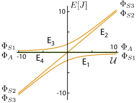
Figure 1: Anyonic-Hubbard-dimer eigenenergies for all three cases of (i) spinless bosonic-based anyons, (ii) spin-1/2 bosonic-based anyons, and (iii) spin-1/2 fermionic-based anyons given by Eq. (13) plus $E_{4}=0$. The limiting $\Phi$ forms for the associated wave functions at ${\cal U}\rightarrow\pm\infty$ are also denoted.

For the two spin-1/2 cases (whether for two bosons or fermions), we seek solutions for states with $S_{z}=0$ (vanishing total-spin projection note ) . In this case, the natural basis set is given by the four kets (note the choice of the ordering of these kets)

$$\ket{\uparrow\downarrow,0},\;\;\ket{\downarrow,\uparrow},\;\;\ket{\uparrow,\downarrow},\;\;\ket{0,\uparrow\downarrow}.$$ (17)

In first quantization, these kets correspond to permanents for bosons and to determinants for fermions. Employing this ket basis, one can derive the following $4\times 4$ matrix Hamiltonians associated with the spin-$1/2$ Hubbard Hamiltonians in Eqs. (7) and (10),

$$H=\left(\begin{array}[]{cccc}U&\mp e^{-i\theta}J&-e^{-i\theta}J&0\\ \mp e^{i\theta}J&0&0&\mp J\\ -e^{i\theta}J&0&0&-J\\ 0&\mp J&-J&U\end{array}\right)$$ (22)

where the upper minus sign in $\mp$ applies for bosons and the bottom plus sign applies for fermions.

The four eigenenergies of the two matrices (22) are given by the three quantities $E_{i}$, $i=1,\ldots,3$ in Eq. (16) and an additional vanishing eigenenergy $E_{4}=0$; they are plotted in Fig. 1 and they are are independent of the statistical angle $\theta$ and the $\mp$ alternation in sign. In contrast, as was also the case of the spinless bosons, the corresponding four normalized eigenvectors do depend on the statistical angle $\theta$; they are given in Appendix B.

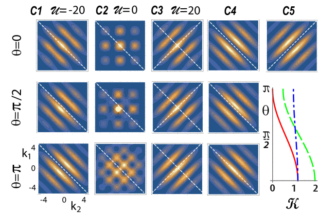
Figure 2: Second-order momentum correlation maps exhibiting signatures of anyonic statistics (i.e., dependence on the statistical angle $\theta$) for two interacting anyonic ultracold atoms trapped in a double well. Columns $C1-C3$: case of the ground state (with energy $E_{1}$) [see Eq. (24)], dependent on both the interaction ${\cal U}$ and the statistical angle $\theta$. Column C1: strong attractive interparticle interaction ${\cal U}=-20$. Column C2: vanishing interparticle interaction, ${\cal U}=0$. Column C3: strong repulsive interparticle interaction, ${\cal U}=20$. Column $C4$: case of the excited state with energy $E_{2}$ [see Eq. (25)], dependent on the statistical angle $\theta$, but independent of the interaction ${\cal U}$. Column $C5$, top frame: case of the excited state with energy $E_{4}=0$ [see Eq. (27)], being independent from both $\theta$ and ${\cal U}$; the wave function of this state is antisymmetric under the exchange of $k_{1}$ and $k_{2}$. Column $C5$, bottom frame: The functions ${\cal K}(\theta)=\pi{\cal G}_{1}^{S}(0,0,\theta)/(4s^{2})$ that correspond to Figs. 2(C1) (red solid line), Figs. 2(C2) (green dashed line), and Figs. 2(C3) (blue dash-dotted line) for the ground state. Top row: $\theta=0$ (pure bosons or fermions). Middle row: $\theta=\pi/2$ (intermediate anyons). Bottom row: $\theta=\pi$ (hard bosons or pseudofermions). The terms hard bosons and pseudofermions reflect the fact that the onsite commutation (anticommutaion) relations do not change as a function of $\theta$, i.e., the onsite exclusion-principle behavior does not transmute from bosonic to fermionic and vice versa. The remaining parameters are: interwell distance, $2d=2$ $\mu$m and width of single-particle orbital, $s=0.2$ $\mu$m. $s$ governs the decay of the interference pattern away from the center of the map, while $1/d$ controls the spacing between the fringes. $k_{1}$ and $k_{2}$ in units of $1/\mu$m. The dashed white lines are a guide to the eye. Blue represents the zero of the color scale. The white color corresponds to the maximum value of ${\cal G}(k_{1},k_{2},\theta)$. (Blue is rendered into black in the printed version.)

III Results: Second-order momentum correlation maps

The spatial far-field interference patterns map linearly onto the second-order momentum correlations characterizing the pure state of the atoms in the source (that is, in the optical-tweezers-generated double-well confinement). To generate the second-order momentum correlation maps ${\cal G}_{i}(k_{1},k_{2},\theta)$, $i=1,\ldots,4$, one needs to transit to the first-quantization formalism, which uses position- or momentum-dependent site-localized orbitals, $\psi_{L}$ and $\psi_{R}$. To this effect, each pure bosonic or fermionic particle in either of the two wells is represented by a displaced Gaussian function bran17 ; bran18 ; yann19 , which equivalently in momentum space is given by

$$\psi_{j}(k)=\frac{2^{1/4}\sqrt{s}}{\pi^{1/4}}e^{-k^{2}s^{2}}e^{id_{j}k},$$ (23)

where again the index $j$ stands for $L$ (left) or $R$ (right); the separation between the two wells is $2d=d_{R}-d_{L}$. The value of the single-particle spatial-extent parameter $s$, as well as the separation $2d$ between the wells are taken in the numerical illustrations (see Fig. 2) to have values (0.2 $\mu$m and 2 $\mu$m, respectively) similar to those used in experimental investigations of 1D trapped ultracold atoms prei18 .

The details of the derivation are given in Appendix C. Here we list the final analytical formulas for the ${\cal G}_{i}(k_{1},k_{2},\theta)$’s, which are independent of the total spin (i.e., whether the state is spinless or a spin singlet or a spin triplet state), and thus are the same for all three cases (i)-(iii). For the ground state, with energy $E_{1}$, one finds the following second-order momentum correlations

$$\begin{split}&{\cal G}_{1}^{S}(k_{1},k_{2},\theta)=\frac{2s^{2}e^{-2s^{2}(k_{1}^{2}+k_{2}^{2})}}{\pi\sqrt{{\cal U}^{2}+16}}\times\\ &\Big{(}{\cal R}({\cal U})\cos^{2}[d(k_{1}-k_{2})]+{\cal R}({-\cal U})\cos^{2}[d(k_{1}+k_{2})+\theta/2]+\\ &8\cos[d(k_{1}-k_{2})]\cos[d(k_{1}+k_{2})+\theta/2]\cos(\theta/2)\Big{)},\end{split}$$ (24)

where ${\cal R}({\cal U})=\sqrt{{\cal U}^{2}+16}+{\cal U}$. The superscript $S$ here, and in Eqs. (25) and (26) below, denotes that the momentum part of the corresponding two-particle wave functions is symmetric under the exchange of the two momenta $k_{1}$ and $k_{2}$; see Appendix C.

For the excited state with energy $E_{2}$, one finds the following second-order momentum correlations

$${\cal G}_{2}^{S}(k_{1},k_{2},\theta)= \frac{4s^{2}}{\pi}e^{-2s^{2}(k_{1}^{2}+k_{2}^{2})}\sin^{2}[d(k_{1}+k_{2})+\theta/2)].$$ (25)

For the excited state with energy $E_{3}$, one finds the following second-order momentum correlations

$$\begin{split}&{\cal G}_{3}^{S}(k_{1},k_{2},\theta)=\frac{2s^{2}e^{-2s^{2}(k_{1}^{2}+k_{2}^{2})}}{\pi\sqrt{{\cal U}^{2}+16}}\times\\ &\Big{(}{\cal R}({-\cal U})\cos^{2}[d(k_{1}-k_{2})]+{\cal R}({\cal U})\cos^{2}[d(k_{1}+k_{2})+\theta/2]-\\ &8\cos[d(k_{1}-k_{2})]\cos[d(k_{1}+k_{2})+\theta/2]\cos(\theta/2)\Big{)},\end{split}$$ (26)

Finally, for the excited state with energy $E_{4}$ [only for the two spin-1/2 cases (ii) and (iii)], one finds the following second-order momentum correlations

$$\begin{split}{\cal G}_{4}^{A}(k_{1},k_{2},\theta)=\frac{4s^{2}}{\pi}e^{-2s^{2}(k_{1}^{2}+k_{2}^{2})}\sin^{2}[d(k_{1}-k_{2})].\end{split}$$ (27)

The superscript $A$ here denotes that the momentum part of the corresponding two-particle wave function is antisymmetric under the exchange of the two momenta $k_{1}$ and $k_{2}$; see Appendix C.

The ${\cal G}_{i}(k_{1},k_{2},\theta)$ expressions above exhibit the following properties: (1) The first three ${\cal G}_{i}$’s ($i=1,2,3$) are associated with two-particle eigenstates whose momentum parts are symmetric under the exchange of the two momenta $k_{1}$ and $k_{2}$. Consequently, the underlying nodal structure does not allow a zero valley along the main diagonal. These three cases depend on the statistical angle $\theta$. Thus their time-of-flight measurement will provide a signature for anyonic statistics. (2) The statistical angle $\theta$ appears only in conjunction with cosine or sine terms containing the sum $k_{1}+k_{2}$ in their arguments. Cosine or sine terms containing only the difference $k_{1}-k_{2}$ of the two momenta are independent of $\theta$. This is a reflection of the fact that the vector solutions of the anyonic matrix Hamiltonians [see Eqs. (A4) and (B3)] contain the phase $e^{i\theta}$ only in the NOON-state component brom10 ; long12 ; lebu15 (of the form $(|2,0\rangle\pm e^{i\theta}|0,2\rangle)/\sqrt{2}$ or $\ket{\uparrow\downarrow,0}\pm e^{i\theta}\ket{0,\uparrow\downarrow}$, see Appendices A-B), and not in the Einstein-Podolski-Rosen-state component shih03 (of the form $|1,1\rangle$ or $\ket{\downarrow,\uparrow}\pm\ket{\uparrow,\downarrow}$). (4) Only the fourth one ($i=4$, corresponding to the constant energy $E_{4}=0$) is associated with a two-particle eigenstate whose momentum part is antisymmetric under the exchange of $k_{1}$ and $k_{2}$; consequently, the undelying nodal structure enforces a zero valley along the main diagonal. This state, which corresponds to two indistinguishable fermions (e.g., two ⁶Li atoms in a triplet excited state) or bosons, is devoid of anyonic statistics.

Fig. 2 displays three cases (corresponding to the ground state and the two excited states with energies $E_{2}$ and $E_{4}$) of second-order momentum correlation maps that illustrate the above properties. Keeping with property (2) above, the variation of the interference patterns as a function of $\theta$ are more intense the larger the ${\cal U}$-dependent contribution of the $k_{1}+k_{2}$ terms in the total ${\cal G}$ (the $k_{1}+k_{2}$ contributions produce interference fringes parallel to the antidiagonal). We note the alternation from a ridge to a valley along the antidiagonal in Fig. 2(C1) (ground state at attractive ${\cal U}=-20$) and vice versa in Fig. 2(C4) ($E_{2}$ state independent of ${\cal U}$). For the ground state in the absence of interactions [Fig. 2(C2)], visible modifications (as a function of $\theta$) of a plaid-type theme persist in the interference patterns. For the case when the $k_{1}+k_{2}$ terms have a small (or vanishing) contribution, the variations of the maps are minimal [see Fig. 2(C3)] [or are absent, see Fig. 2(C5), top frame]; in this case, the dominance of the $\theta$-independent $k_{1}-k_{2}$ contributing terms is reflected in fringes parallel to the main diagonal. The bottom frame in the C5 column offers a complementary view of the $\theta$ dependence by plotting the curves ${\cal K}(\theta)=\pi{\cal G}_{1}^{S}(k_{1}=0,k_{2}=0,\theta)/(4s^{2})$ that correspond to Figs. 2(C1), Figs. 2(C2), and Figs. 2(C3) for the ground state.

For completeness, the case of the excited state with energy $E_{3}$ is presented in Appendix D; see Fig. 3.

IV Summary

In summary, the paper introduced the subject of matter-wave interferometry of massive and interacting anyons that can be realized with trapped 1D ultracold atoms in optical lattices. Furthermore, it analyzed the pertinent signatures in the framework of time-of-flight experiments, and it established analogies with the interferometry of massless and noninteracting photonic anyons in waveguide lattices brom10 ; long12 ; lebu15 . In particular, for two ultracold-atom anyons in a double-well confinement, this analogy is reflected in the fact that the NOON-state component of the massive bianyon is also of the form $(|2,0\rangle\pm e^{i\theta}|0,2\rangle)/\sqrt{2}$, where $\theta$ is the statistical angle determining the commutation (anticommutation) relations for the anyonic exchange.

Appendix A Solution for two bosonic-based spinless anyons

Using the bosonic basis kets

$$\ket{2,0},\;\;\ket{1,1},\;\;\ket{0,2},$$ (28)

where $\ket{n_{L},n_{R}}$ (with $n_{L}+n_{R}=2$) corresponds to a permanent with $n_{L}$ ($n_{R}$) particles in the $L$ ($R$) site, one derives the following matrix Hamiltonian associated with the anyonic Hubbard Hamiltonian in Eq. (4)

$$H=\left(\begin{array}[]{cccc}U&-\sqrt{2}e^{-i\theta}J&0\\ -\sqrt{2}e^{i\theta}J&0&-\sqrt{2}J\\ 0&-\sqrt{2}J&U\\ \end{array}\right).$$ (32)

The three eigenenergies of the matrix (32) are given by

$$\begin{split}E_{1}&=\frac{J}{2}({\cal U}-\sqrt{{\cal U}^{2}+16})\\ E_{2}&=J{\cal U}=U\\ E_{3}&=\frac{J}{2}({\cal U}+\sqrt{{\cal U}^{2}+16}),\end{split}$$ (33)

where ${\cal U}=U/J$. These eigenenergies are plotted in Fig. 1.

The corresponding three normalized eigenvectors are

$$\begin{split}{\cal V}_{1}&=\{{\cal B}({\cal U})e^{-i\theta}/\sqrt{2},\;{\cal A}({\cal U}),\;{\cal B}({\cal U})/\sqrt{2}\}^{T}\\ {\cal V}_{2}&=\{e^{-i\theta}/\sqrt{2},\;0,\;-1/\sqrt{2}\}^{T}\\ {\cal V}_{3}&=\{{\cal E}({\cal U})e^{-i\theta}/\sqrt{2},\;{\cal D}({\cal U}),\;{\cal E}({\cal U})/\sqrt{2}\}^{T},\end{split}$$ (34)

where the coefficients ${\cal A}$, ${\cal B}$, ${\cal D}$, and ${\cal E}$ are given by

$$\begin{split}{\cal A}({\cal U})&=\frac{{\cal U}+\sqrt{{\cal U}^{2}+16}}{\sqrt{2}\sqrt{{\cal U}^{2}+{\cal U}\sqrt{{\cal U}^{2}+16}+16}},\\ {\cal B}({\cal U})&=\frac{4}{\sqrt{2}\sqrt{{\cal U}^{2}+{\cal U}\sqrt{{\cal U}^{2}+16}+16}},\\ {\cal D}({\cal U})&=-{\cal A}(-{\cal U}),\\ {\cal E}({\cal U})&={\cal B}(-{\cal U}).\end{split}$$ (35)

Appendix B Solution for two spin-$1/2$ anyons

We seek solutions for states with $S_{z}=0$ (vanishing total spin projection). In this case, the natural basis set is given by the four kets (note the choice of the ordering of these kets)

$$\ket{\uparrow\downarrow,0},\;\;\ket{\downarrow,\uparrow},\;\;\ket{\uparrow,\downarrow},\;\;\ket{0,\uparrow\downarrow}.$$ (36)

In first quantization, these kets correspond to permanents for bosons and to determinants for fermions. Employing this basis, one can derive the following $4\times 4$ matrix Hamiltonians associated with the spin-$1/2$ Hubbard Hamiltonians in Eqs. (7) and (10),

$$H=\left(\begin{array}[]{cccc}U&\mp e^{-i\theta}J&-e^{-i\theta}J&0\\ \mp e^{i\theta}J&0&0&\mp J\\ -e^{i\theta}J&0&0&-J\\ 0&\mp J&-J&U\end{array}\right)$$ (41)

where the upper minus sign in $\mp$ applies for bosons and the bottom plus sign applies for fermions.

The four eigenenergies of the matrices (41) are given by the quantities $E_{i}$, $i=1,\ldots,3$ in Eq. (33) and $E_{4}=0$; they are independent of the $\mp$ alternation in sign. The corresponding four normalized eigenvectors are

$$\begin{split}{\cal V}_{1}&=\{{\cal B}({\cal U})e^{-i\theta}/\sqrt{2},\;\pm{\cal A}({\cal U})/\sqrt{2},\;{\cal A}({\cal U})/\sqrt{2},\;{\cal B}({\cal U})/\sqrt{2}\}^{T}\\ {\cal V}_{2}&=\{e^{-i\theta}/\sqrt{2},\;0,\;0,\;-1/\sqrt{2}\}^{T}\\ {\cal V}_{3}&=\{{\cal E}({\cal U})e^{-i\theta}/\sqrt{2},\;\pm{\cal D}({\cal U})/\sqrt{2},\;{\cal D}({\cal U})/\sqrt{2},\;{\cal E}({\cal U})/\sqrt{2}\}^{T}\\ {\cal V}_{4}&=\{0,\;1/\sqrt{2},\;\mp 1/\sqrt{2},\;0\}^{T},\end{split}$$ (42)

where the upper sign (in $\pm$ or $\mp$) applies for bosons and the bottom sign applies for fermions.

Appendix C Second-order momentum correlation maps

To generate the second-order momentum correlation maps, one needs to transit from the ket notation to the wave function notation by employing the single-particle momentum-dependent site-localized orbitals $\psi_{L}(k)$ and $\psi_{R}(k)$ given in Eq. (23). Indeed, in the first representation, the kets correspond to permanents for bosons or to determinants for fermions made of the $\psi_{L}(k)$ and $\psi_{R}(k)$ orbitals.

One finds the following correspondence for spinless anyons

$$\begin{split}&\ket{1,1}\rightarrow\Phi_{S1}(k_{1},k_{2})\\ &e^{-i\theta}\ket{2,0}-\ket{0,2}\rightarrow\sqrt{2}\Phi_{S2}(k_{1},k_{2},\theta)\\ &e^{-i\theta}\ket{2,0}+\ket{0,2}\rightarrow\sqrt{2}\Phi_{S3}(k_{1},k_{2},\theta),\end{split}$$ (43)

and

$$\begin{split}&\ket{\uparrow,\downarrow}\pm\ket{\downarrow,\uparrow}\rightarrow\sqrt{2}\Phi_{S1}(k_{1},k_{2}){\cal X}_{1}\\ &e^{-i\theta}\ket{\uparrow\downarrow,0}-\ket{0,\uparrow\downarrow}\rightarrow\sqrt{2}\Phi_{S2}(k_{1},k_{2},\theta){\cal X}_{2}\\ &e^{-i\theta}\ket{\uparrow\downarrow,0}+\ket{0,\uparrow\downarrow}\rightarrow\sqrt{2}\Phi_{S3}(k_{1},k_{2},\theta){\cal X}_{3}\\ &\ket{\uparrow,\downarrow}\mp\ket{\downarrow,\uparrow}\rightarrow\sqrt{2}\Phi_{A}(k_{1},k_{2}){\cal X}_{4}.\end{split}$$ (44)

for spin-$1/2$ anyons, where the upper sign applies to bosonic-based anyons and the bottom sign applies to fermionic-based ones. ${\cal X}_{i}=\chi(1,0)$ for $i=1,2,3$ and ${\cal X}_{4}=\chi(0,0)$ for bosons and ${\cal X}_{i}=\chi(0,0)$, $i=1,2,3$ and ${\cal X}_{4}=\chi(1,0)$ for fermions; $\chi(0,0)$ and $\chi(1,0)$ are the singlet and triplet spin eigenfunctions, respectively. The $\Phi$ functions are as follows:

$$\begin{split}&\Phi_{S1}(k_{1},k_{2})=\big{(}\psi_{L}(k_{1})\psi_{R}(k_{2})+\psi_{R}(k_{1})\psi_{L}(k_{2})\big{)}/\sqrt{2}=\frac{2s}{\sqrt{\pi}}e^{-s^{2}(k_{1}^{2}+k_{2}^{2})}\cos[d(k_{1}-k_{2})],\\ &\Phi_{S2}(k_{1},k_{2},\theta)=\big{(}e^{-i\theta}\psi_{L}(k_{1})\psi_{L}(k_{2})-\psi_{R}(k_{1})\psi_{R}(k_{2})\big{)}/\sqrt{2}=-i\frac{2s}{\sqrt{\pi}}e^{-s^{2}(k_{1}^{2}+k_{2}^{2})}e^{-i\theta/2}\sin[d(k_{1}+k_{2})+\theta/2)],\\ &\Phi_{S3}(k_{1},k_{2},\theta)=\big{(}e^{-i\theta}\psi_{L}(k_{1})\psi_{L}(k_{2})+\psi_{R}(k_{1})\psi_{R}(k_{2})\big{)}/\sqrt{2}=\frac{2s}{\sqrt{\pi}}e^{-s^{2}(k_{1}^{2}+k_{2}^{2})}e^{-i\theta/2}\cos[d(k_{1}+k_{2})+\theta/2)],\\ &\Phi_{A}(k_{1},k_{2})=\big{(}\psi_{L}(k_{1})\psi_{R}(k_{2})-\psi_{R}(k_{1})\psi_{L}(k_{2})\big{)}/\sqrt{2}=-i\frac{2s}{\sqrt{\pi}}e^{-s^{2}(k_{1}^{2}+k_{2}^{2})}\sin[d(k_{1}-k_{2})].\end{split}$$ (45)

For the ground state, with energy $E_{1}$, one finds the following second-order momentum correlations

$$\begin{split}&{\cal G}_{1}^{S}(k_{1},k_{2},\theta)=|{\cal A}({\cal U})\Phi_{S1}(k_{1},k_{2})+{\cal B}({\cal U})\Phi_{S3}(k_{1},k_{2},\theta)|^{2}=\\ &\frac{4s^{2}}{\pi}e^{-2s^{2}(k_{1}^{2}+k_{2}^{2})}\Big{(}{\cal A}({\cal U})^{2}\cos^{2}[d(k_{1}-k_{2})]+{\cal B}({\cal U})^{2}\cos^{2}[d(k_{1}+k_{2})+\theta/2]+\\ &2{\cal A}({\cal U}){\cal B}({\cal U})\cos[d(k_{1}-k_{2})]\cos[d(k_{1}+k_{2})+\theta/2]\cos(\theta/2)\Big{)}.\end{split}$$ (46)

For the excited state with energy $E_{2}$, one finds the following second-order momentum correlations

$$\begin{split}{\cal G}_{2}^{S}(k_{1},k_{2},\theta)=|\Phi_{S2}(k_{1},k_{2},\theta)|^{2}=\frac{4s^{2}}{\pi}e^{-2s^{2}(k_{1}^{2}+k_{2}^{2})}\sin^{2}[d(k_{1}+k_{2})+\theta/2)].\end{split}$$ (47)

For the excited state with energy $E_{3}$, one finds the following second-order momentum correlations

$$\begin{split}&{\cal G}_{3}^{S}(k_{1},k_{2},\theta)=|-{\cal A}(-{\cal U})\Phi_{S1}(k_{1},k_{2})+{\cal B}(-{\cal U})\Phi_{S3}(k_{1},k_{2},\theta)|^{2}=\\ &\frac{4s^{2}}{\pi}e^{-2s^{2}(k_{1}^{2}+k_{2}^{2})}\Big{(}{\cal A}(-{\cal U})^{2}\cos^{2}[d(k_{1}-k_{2})]+{\cal B}(-{\cal U})^{2}\cos^{2}[d(k_{1}+k_{2})+\theta/2]\\ &-2{\cal A}(-{\cal U}){\cal B}(-{\cal U})\cos[d(k_{1}-k_{2})]\cos[d(k_{1}+k_{2})+\theta/2]\cos(\theta/2)\Big{)}.\end{split}$$ (48)

Finally, for the excited state with energy $E_{4}=0$, one finds the following second-order momentum correlations

$$\begin{split}{\cal G}^{A}_{4}(k_{1},k_{2},\theta)=|\Phi_{A}(k_{1},k_{2})|^{2}=\frac{4s^{2}}{\pi}e^{-2s^{2}(k_{1}^{2}+k_{2}^{2})}\sin^{2}[d(k_{1}-k_{2})].\end{split}$$ (49)

Figure 3: Second-order momentum correlations of the excited state with energy $E_{3}$ of two interacting anyonic ultracold atoms trapped in a double well [see Eq. (26)], demonstrating dependence on the statistical angle $\theta$. Top row: $\theta=0$ (pure bosons or fermions). Middle row: $\theta=\pi/2$ (intermediate anyons). Bottom row: $\theta=\pi$ (hard bosons or pseudofermions). Column C1: attractive interparticle interaction ${\cal U}=-20$. Column C2: vanishing interparticle interaction, ${\cal U}=0$. Column C3: repulsive interparticle interaction, ${\cal U}=20$. The remaining parameters are: interwell distance, $2d=2$ $\mu$m and width of single-particle orbital, $s=0.2$ $\mu$m. $k_{1}$ and $k_{2}$ in units of $1/\mu$m. The dashed white lines are a guide to the eye. Blue represents the zero of the color scale. The white color corresponds to the maximum value of ${\cal G}_{3}^{S}(k_{1},k_{2},\theta)$. (Blue is rendered into black in the printed version.)

With regard to the derivation of the expressions in Eqs. (46)$-$(49), we note that, generally, the second-order (two-particle) space density $\rho(x_{1},x_{1}^{\prime},x_{2},x_{2}^{\prime})$ for an $N$-particle system is defined as an integral over the product of the many-body wave function $\Psi(x_{1},x_{2},\ldots,x_{N})$ and its complex conjugate $\Psi^{*}(x_{1}^{\prime},x_{2}^{\prime},\ldots,x_{N})$, taken over the coordinates $x_{3},\ldots,x_{N}$ of $N-2$ particles. To obtain the second-order space correlation function, ${\cal G}(x_{1},x_{2})$, one sets $x_{1}^{\prime}=x_{1}$ and $x_{2}^{\prime}=x_{2}$. The second-order momentum correlation function ${\cal G}(k_{1},k_{2})$ is obtained via a Fourier transform (from real space to momentum space) of the two-particle space density $\rho(x_{1},x_{1}^{\prime},x_{2},x_{2}^{\prime})$ bran17 ; bran18 . In the case of $N=2$, the above general definition reduces to a simple expression for the two-particle correlation functions, as the modulus square of the two-particle wave function itself; this applies in both cases whether the two-particle wave function is written in space or in momentum coordinates. This simpler second approach was followed here for deriving above the second-order momentum correlations for two anyons.
    

Appendix D Plots of correlation maps for the excited state with energy $E_{3}$

Fig. 3 displays the second-order correlation maps for the excited state with energy $E_{3}$. It complements Fig. 2 where the corresponding maps for the three eigenstates with energies $E_{1}$, $E_{2}$, and $E_{4}=0$ were displayed. For a description of these states as a function of the interparticle on-site interaction, ${\cal U}$, see Fig. 1.

References

- (1) I. Bloch, J. Dalibard, and W. Zwerger, Many-body physics with ultracold gases, Rev. Mod. Phys. 80, 885 (2008).
- (2) J.I. Cirac and P. Zoller, Goals and opportunities in quantum simulation, Nature Phys. 8, 264–266 (2012).
- (3) S. Fölling, F. Gerbier, A. Widera, O. Mandel, T. Gericke, and I. Bloch, Spatial quantum noise interferometry in expanding ultracold atom clouds, Nature 434, 491 (2005).
- (4) A.M. Kaufman, B.J. Lester, C.M. Reynolds, M.L. Wall, M. Foss-Feig, K.R.A. Hazzard, A.M. Rey, and C.A. Regal, Two-particle quantum interference in tunnel-coupled optical tweezers, Science 345, 306 (2014).
- (5) A.M.Kaufman, M.C. Tichy, F. Mintert, A.M. Rey and C.A.Regal, The Hong-Ou-Mandel Effect With Atoms, Adv. At. Mol. Opt. Phys. 67, 377 (2018).
- (6) R. Lopes, A. Imanaliev, A. Aspect, M. Cheneau, D. Boiron, and C.I. Westbrook, Atomic Hong-Ou-Mandel experiment, Nature 520, 66 (2015).
- (7) R. Islam, R. Ma, Ph. M. Preiss, M.E. Tai, A. Lukin, M. Rispoli, and M. Greiner, Measuring entanglement entropy in a quantum many-body system, Nature 528, 77 (2015).
- (8) B.B. Brandt, C. Yannouleas, and U. Landman, Two-point momentum correlations of few ultracold quasi-one-dimensional trapped fermions: Diffraction patterns, Phys. Rev. A 96, 053632 (2017).
- (9) B.B. Brandt, C. Yannouleas, and U. Landman, Interatomic interaction effects on second-order momentum correlations and Hong-Ou-Mandel interference of double-well-trapped ultracold fermionic atoms, Phys. Rev. A 97, 053601 (2018).
- (10) C. Yannouleas, B.B. Brandt, and U. Landman, Interference, spectral momentum correlations, entanglement, and Bell inequality for a trapped interacting ultracold atomic dimer: Analogies with biphoton interferometry, Phys. Rev. A 99, 013616 (2019).
- (11) M. Bonneau, W.J. Munro, K. Nemoto, and Jörg Schmiedmayer, Characterizing twin-particle entanglement in double-well potentials, Phys. Rev. A 98, 033608 (2018).
- (12) M.J. Hartmann, F.G.S.L. Brandao, and M.B. Plenio, Strongly interacting polaritons in coupled arrays of cavities, Nat. Phys. 2, 849 (2006),
- (13) A.D. Greentree, C. Tahan, J.H. Cole, and L.C.L. Hollenberg, Quantum phase transitions of light, Nat. Phys. 2, 856 (2006).
- (14) D.G. Angelakis, M.F. Santos, and S. Bose, Photonblockade-induced Mott transitions and XY spin models in coupled cavity arrays, Phys. Rev. A 76 031805 (2007).
- (15) D. Rossini and R. Fazio, Mott-insulating and glassy phases of polaritons in 1D arrays of coupled cavities. Phys. Rev. Lett. 99, 186401 (2007).
- (16) Y. Bromberg, Y. Lahini, and Y. Silberberg, Bloch oscillations of path-entangled photons, Phys. Rev. Lett. 105, 263604 (2010).
- (17) S. Longhi and G. Della Valle, Anyons in one-dimensional lattices: a photonic realization, Opt. Lett. 37, 2160 (2012).
- (18) M. Lebugle, M. Gräfe, R. Heilman, A. Perez-Leija, S. Nolte, and A. Szameit, Experimental observation of N00N state Bloch oscillations, Nat. Commun. 6, 8273 (2015).
- (19) C. Noh and D.G. Angelakis, Quantum simulations and many-body physics with light, Rep. Prog. Phys. 80, 016401 (2017).
- (20) J.M. Leinaas and J. Myrheim, On the theory of identical particles, Il Nuovo Cimento B 37, 1 (1977).
- (21) F. Wilczek, Quantum mechanics of fractional-spin particles, Phys. Rev. Lett. 49, 957 (1982).
- (22) A.Yu. Kitaev, Fault-tolerant quantum computation by anyons, Ann. Phys. (N.Y.) 303, 2 (2003).
- (23) J.K. Pachos, Introduction to topological quantum computation, (Cambridge University Press, 2012)
- (24) B. Rosenow, I. P. Levkivskyi, and B. I. Halperin, Current Correlations from a Mesoscopic Anyon Collider, Phys. Rev. Lett. 116, 156802 (2016).
- (25) T. Dubček, B. Klajn, R. Pezer, H. Buljan, and D. Jukić, Quasimomentum distribution and expansion of an anyonic gas, Phys. Rev. A 97, 011601(R) (2018).
- (26) R.O. Umucalilar, E. Macaluso, T. Comparin, and I. Carusotto, Time-of-flight measurements as a possible method to observe anyonic statistics, Phys. Rev. Lett. 120, 230403 (2018).
- (27) T. Keilmann, S. Lanzmich, I. McCulloch, and M. Roncaglia, Statistically induced phase transitions and anyons in 1D optical lattices, Nat. Commun. 2, 361 (2011).
- (28) S. Greschner and L. Santos, Anyon Hubbard model in one-dimensional optical lattices, Phys. Rev. Lett. 115, 053002 (2015).
- (29) Ch. Sträter, S.C.L. Srivastava, and A. Eckardt, Floquet realization and signatures of one-dimensional anyons in an optical lattice, Phys. Rev. Lett. 117, 205303 (2016).
- (30) G. Tang, S. Eggert, and A. Pelster, Ground-state properties of anyons in a one-dimensional lattice, New J. Phys. 17, 123016 (2015).
- (31) J. Arcila-Forero, R. Franco, and J. Silva-Valencia, Critical points of the anyon-Hubbard model, Phys. Rev. A 94, 013611 (2016).
- (32) W. Zhang, S. Greschner, E. Fan, T.C. Scott, and Y. Zhang, Ground-state properties of the one-dimensional unconstrained pseudo-anyon Hubbard model, Phys. Rev. A 95, 053614 (2017).
- (33) F. Lange, S. Ejima, and H. Fehske, Anyonic Haldane Insulator in One Dimension, Phys. Rev. Lett. 118, 120401 (2017).
- (34) F. Liu, J. R. Garrison, D.-L. Deng, Z.-X. Gong, and A. V. Gorshkov, Asymmetric Particle Transport and Light-Cone Dynamics Induced by Anyonic Statistics, Phys. Rev. Lett. 121, 250404 (2018).
- (35) Z.-W. Zuo, G.-L. Li, and L. Li, Statistically induced topological phase transitions in a one-dimensional superlattice anyon-Hubbard model, Phys. Rev. B 97, 115126 (2018).
- (36) J. Arcila-Forero, R. Franco, and J. Silva-Valencia, Three-body-interaction effects on the ground state of one-dimensional anyons, Phys. Rev. A 97, 023631 (2018).
- (37) L. Mandel, Quantum effects in one-photon and two-photon interference, Rev. Mod. Phys. 71, S274 (1999).
- (38) Y. H. Shih, An Introduction to Quantum Optics: Photon and Biphoton Physics (CRC Press, Boca Raton, Florida, 2011)
- (39) Z. Y. Ou, Multi-photon Quantum Interference (Springer, New York, 2007).
- (40) S. Murmann, A. Bergschneider, V. M. Klinkhamer, G. Zürn, T. Lompe, and S. Jochim, Two fermions in a double well: Exploring a fundamental building block of the Hubbard model, Phys. Rev. Lett. 114, 080402 (2015).
- (41) Ph. M. Preiss, J. H. Becher, R. Klemt, V. Klinkhamer, A. Bergschneider, and S. Jochim, High-Contrast Interference of Ultracold Fermions, Phys. Rev. Lett. 122, 143602 (2019).
- (42) A. Bergschneider, V. M. Klinkhamer, J. H. Becher, R. Klemt, L. Palm, G. Zürn, S. Jochim, and Ph. M. Preiss, Experimental characterization of two-particle entanglement through position and momentum correlations, Nature Phys. 15, 640 (2019), https://www.nature.com/articles/s41567-019-0508-6.
- (43) E. Altman, E. Demler, and M. D. Lukin, Probing many-body states of ultracold atoms via noise correlations, Phys. Rev. A 70, 013603 (2004).
- (44) T. Jeltes, J. M. McNamara, W. Hogervorst, W. Vassen, V. Krachmalnicoff, M. Schellekens, A. Perrin, H. Chang, D. Boiron, A. Aspect, and C. I. Westbrook, Comparison of the Hanbury Brown-Twiss effect for bosons and fermions, Nature 445, 402 (2007).
- (45) S. S. Hodgman, R. G. Dall, A. G. Manning, K. G. H. Baldwin, and A. G. Truscott, Direct Measurement of Long-Range Third-Order Coherence in Bose-Einstein Condensates, Science 331, 1046 (2011).
- (46) A. G. Manning, Wu RuGway, S. S. Hodgman, R. G. Dall, K. G. H. Baldwin, and A. G. Truscott, Third-order spatial correlations for ultracold atoms, New J. Phys. 15, 013042 (2013).
- (47) R. G. Dall, A. G. Manning, S. S. Hodgman, Wu RuGway, K. V. Kheruntsyan, and A. G. Truscott, Ideal -body correlations with massive particles, Nature Phys. 9, 341 (2013).
- (48) S. S. Hodgman, R. I. Khakimov, R. J. Lewis-Swan, A. G. Truscott, and K. V. Kheruntsyan, Solving the Quantum Many-Body Problem via Correlations Measured with a Momentum Microscope, Phys. Rev. Lett. 118, 240402 (2017).
- (49) R. J. Lewis-Swan and K. V. Kheruntsyan, Proposal for demonstrating the Hong-Ou-Mandel effect with matter waves, Nature Commun. 5, 3752 (2014).
- (50) O. Carnal and J. Mlynek, Young’s double slit experiment with atoms: A simple atom interferometer, Phys. Rev. Lett. 66, 2689 (1991).
- (51) A. D. Cronin, J. Schmiedmayer, and D. E. Pritchard, Optics and interferometry with atoms and molecules, Rev. Mod. Phys. 81, 1051 (2009).
- (52) P. R. Berman, Atom Interferomerty (Academic Press, San Diego, 1997).
- (53) P. Berg, S. Abend, G. Tackmann, C. Schubert, E. Giese, W. P. Schleich, F. A. Narducci, W. Ertmer, and E. M. Rasel, Composite-Light-Pulse Technique for High-Precision Atom Interferometry, Phys. Rev. Lett. 114, 063002 (2015).
- (54) C.D. Batista and G. Ortiz, Algebraic approach to interacting quantum systems, Adv. Phys. 53, 1 (2004).
- (55) The spin-polarized cases (, ) map to the cases of spinless particles. Namely, for bosons, there are three basis kets , , , and the exposition follows the case of two spinless bosons. For fermions, the fully polarized case is trivial, because there is only one basis ket , leading to a single-determinantal wave function with vanishing energy, and to a second-order momentum correlation given by Eq. (27).
- (56) Y.H. Shih, Entangled biphoton source - property and preparation, Rep. Prog. Phys. 66, 1009 (2003).