A Discontinuous Galerkin Method by Patch Reconstruction for Elliptic Interface Problem on Unfitted Mesh

Abstract.

We propose a discontinuous Galerkin (DG) method to approximate the elliptic interface problem on unfitted mesh using a new approximation space. The approximation space is constructed by patch reconstruction with one degree of freedom per element. The optimal error estimates in both $L^{2}$ norm and DG energy norm are obtained, without restrictions on how the interface intersects the elements in the mesh. The stability near the interface is ensured by the patch reconstruction and no special numerical flux is required. The convergence order by numerical results in both 2D and 3D agrees with the error estimates perfectly. More than enjoying the advantages of DG method, the new method may achieve even better efficiency in number of degree of freedom than the conforming finite element method as illustrated by our numerical examples.

keywords: Elliptic interface problems, Patch reconstructed, Discontinuous Galerkin method, Unfitted mesh.

1. Introduction

In the last decades, numerical methods for the elliptic interface problem have attracted pervasive attention since the pioneering work of Peskin [41], for example, the immersed interface method by LeVeque and Li [28, 33], Mayo’s method on irregular regions [38], the method in [53] with second-order accuracy in the $L^{\infty}$ norm. In the finite difference fold, we also refer to [35, 21, 22, 16, 11, 40] for some other interesting methods. Meanwhile, finite element (FE) method is also popular for solving the interface problem. Based on the geometrical relationship between the grid and the interface, FE methods could be classified into two categories: interface-fitted method and interface-unfitted method. The body-fitted grid enforces the mesh to align with the interface to render a high-order accurate approximation [12, 6]. However, generating a fitted mesh with satisfied quality is sometimes a nontrivial and time-consuming task [50, 51]. Therefore, there are some techniques for FE methods based on unfitted grid. The unfitted FE method can date back to the [5], which introduced a penalty term to weakly enforce the jump on the interface. Li proposed the immersed FE method in [32], which processes a better approximate solution by modifying the basis functions near interface to capture the jump of the solution. We refer to [3, 34, 2, 48, 10, 17] for some recent works. Let us note that the extended FE method is also a popular discretization method [7].

In 2002, A. Hansbo and P. Hansbo proposed an unfitted FE method with the piecewise linear space and proved an optimal order of convergence [20]. The numerical solution comes from separate solutions defined on each subdomain and the jump conditions are imposed weakly by Nitsche’s method. Wadbro et al. [46] developed a uniformly well-conditioned FE method based on Nitsche’s method. Wu and Xiao [23, 50] presented a $hp$ unfitted FE method, which is extended to the three dimensional case. To achieve high-order accuracy and enjoy additional flexibility, some authors tried to apply DG method to the elliptic interface problem, for example the local DG method in [18], the hybridizable DG method in [25] on fitted mesh, and the $hp$ DG method in [37] on unfitted mesh.

Though high-order accuracy can be obtained, solid difficulties remain for DG methods in solving problems with complex interfaces. To fit curved interfaces, Cangiani et al. [9] introduced elements with curved faces to give an adaptive DG method recently. As one of the latest work on unfitted mesh, Burman and Ern [8] proposed a hybrid high-order method, while an extra assumption on the meshes are required to ensure the mesh cells are cut favorably by the interface [37]. In this paper, we are trying to propose a DG method on unfitted mesh for the interface problem still using Nitsche’s method. The novel point is that we adopt a new approximation space by patch reconstruction with one degree of freedom (DOF) per element following the methodology in [30, 29]. The new space may be regarded as a subspace of the approximation space used in [37]. Thanks to the flexibility in choosing reconstruction patches, we may allow the interface to intersect elements in a very general manner, in comparison to the methods in [8, 37]. Following the standard DG discretization, the elliptic interface problem is approximated by using a symmetric interior penalty bilinear form with a Nitsche-type penalization at the interface. The optimal error estimate is then derived in both DG energy norm and $L^{2}$ norm. The patch reconstruction can provide the stability near the interface and no cut-dependent numerical flux is used. We note that the idea of using the patch of interface elements to improve the numerical stability can also be found in [19, 13, 23, 17]. In addition, the classical DG methods for elliptic problems were challenged [24, 55] since it may use more DOFs than traditional conforming FE methods. As a new observation, we demonstrate by numerical examples that using our new approximation space, one needs much less DOFs than classical DG methods. For high-order approximations, number of DOFs can be even less than conforming FE methods to achieve the same numerical error.

The rest of this paper is organized as follows. In Section 2, we introduce the reconstruction operator and the new approximation space, and we also give the basic properties of the approximation space. In Section 3, the approximation to the elliptic interface problem is proposed and we derive the optimal error estimate in DG energy norm and $L^{2}$ norm. In Section 4, we present a lot of numerical examples to verify the error estimate in Section 3. To show the performance of our method in efficiency, we make a comparison of number of DOFs with respect to the numerical error between different methods. We also solve a problem that admits solutions with low regularities to illustrate the robustness of our method.

2. Approximation Space

Let $\Omega\subset\mathbb{R}^{d}$, $d=2$ or $3$, be a convex and polygonal (polyhedral) domain with boundary $\partial\Omega$ and let $\Gamma$ be a $C^{2}$-smooth interface which divides $\Omega$ into two open sets $\Omega_{0}$ and $\Omega_{1}$ satisfying $\Omega_{0}\cap\Omega_{1}=\varnothing,\ \overline{\Omega}=\overline{\Omega}_{0}\cup\overline{\Omega}_{1}$ and $\Gamma=\overline{\Omega}_{0}\cap\overline{\Omega}_{1}$. We denote by $\mathcal{T}_{h}$ a partition of $\Omega$ into polygonal (polyhedral) elements. Here we do not require the faces of elements in $\mathcal{T}_{h}$ align with the interface (see Fig 1).

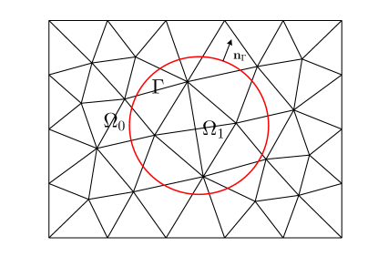
Figure 1. A sample domain and unfitted mesh for $d=2$.

Let $\mathcal{E}^{\circ}_{h}$ be the set of all interior faces of $\mathcal{T}_{h}$, $\mathcal{E}^{b}_{h}$ the set of the faces on $\partial\Omega$ and then $\mathcal{E}_{h}=\mathcal{E}_{h}^{\circ}\cup\mathcal{E}_{h}^{b}$. We set

$$h_{K}=\text{diam}(K),\quad\forall K\in\mathcal{T}_{h},\quad h_{e}=|e|,\quad\forall e\in\mathcal{E}_{h},$$

and we denote by $h$ the biggest one among the diameters of all elements in $\mathcal{T}_{h}$. We assume that $\mathcal{T}_{h}$ is share-regular in the sense of satisfying the conditions introduced in [4], which are: there exist

• two positive numbers $N$ and $\sigma$ which are independent of mesh size $h$;

• a compatible sub-decomposition $\widetilde{\mathcal{T}}_{h}$ into shape-regular triangles (tetrahedrons);

such that

• any polygon (polyhedron) $K\in\mathcal{T}_{h}$ admits a decomposition $\widetilde{\mathcal{T}}_{h|K}$ which has less than $N$ shape-regular triangles (tetrahedrons);

• the share-regularity of $\widetilde{K}\in\widetilde{\mathcal{T}}_{h}$ follows [14]: the ratio between $h_{\widetilde{K}}$ and $\rho_{\widetilde{K}}$ is bounded by $\sigma$: $h_{\widetilde{K}}/\rho_{\widetilde{K}}\leq\sigma$ where $\rho_{\widetilde{K}}$ is the radius of the largest ball inscribed in $\widetilde{K}$.

The above regularity requirements could bring some useful consequences which are trivial to verify [4]:

1. there exists a constant $\rho_{v}$ that only depends on $N$ and $\sigma$ such that $\rho_{v}h_{K}\leq h_{e}$ for every element $K$ and every edge $e$ of $K$.

2. there exists a constant $\rho_{s}$ that only depends on $N$ and $\sigma$ such that for every element $K$ the following holds true

   $$\rho_{s}\max_{\widetilde{K}\in\Delta(K)}h_{\widetilde{K}}\leq h_{K},$$

   where $\Delta(K)=\left\{K^{\prime}\in\mathcal{T}_{h}\ |\ K^{\prime}\cap K\neq\varnothing\right\}$ is the collection of the elements touching $K$.

3. there exists a constant $\tau$ that only depends on $N$ and $\sigma$ such that for every element $K$, there is a disk (ball) inscribed in $K$ with center at the point $\boldsymbol{z}_{K}\in K$ and the radius $\tau h_{K}$.

4. [Trace inequality] there exists a constant $C$ such that

   (1) $$\|v\|_{L^{2}(\partial K)}^{2}\leq C\left(h_{K}^{-1}\|v\|_{L^{2}(K)}^{2}+h_{K}\|\nabla v\|_{L^{2}(K)}^{2}\right),\quad\forall v\in H^{1}(K).$$

5. [Inverse inequality] there exists a constant $C$ such that

   (2) $$\|\nabla v\|_{L^{2}(K)} \leq Ch_{K}^{-1}\|v\|_{L^{2}(K)},\quad\forall v\in\mathbb{P}_{m}(K),$$

   where $\mathbb{P}_{m}(\cdot)$ denotes the polynomial space of degree less than $m$.

Let us note that throughout the paper, $C$ and $C$ with a subscript are generic constants that may be different from line to line but are independent of the mesh size $h$ and how the interface cuts the mesh. Given a bounded domain $D\subset\mathbb{R}^{d}$ and an integer $r\geq 0$, we would use the standard notations and definitions for the spaces $H^{r}(D)$, $L^{r}(D)$ and their corresponding inner products and norms. Then we will use the following notations related to the partition:

$$e^{0} =e\cap\Omega_{0}, \quad e^{1}=e\cap\Omega_{1},\quad\forall e\in\mathcal{E}_{h},$$

$$K^{0} =K\cap\Omega_{0}, \quad K^{1}=K\cap\Omega_{1},\quad\forall K\in\mathcal{T}_{h},$$

$$(\partial K)^{0} =\partial K\cap\Omega_{0}, \quad(\partial K)^{1}=\partial K\cap\Omega_{1},\quad\forall K\in\mathcal{T}_{h},$$

$$\mathcal{T}_{h}^{0} =\left\{K\in\mathcal{T}_{h}\ |\ |K^{0}|>0\right\},\quad \mathcal{T}_{h}^{1}=\left\{K\in\mathcal{T}_{h}\ |\ |K^{1}|>0\right\},$$

$$\mathcal{E}_{h}^{0} =\left\{e\in\mathcal{E}_{h}\ |\ |e^{0}|>0\right\},\quad \mathcal{E}_{h}^{1}=\left\{e\in\mathcal{E}_{h}\ |\ |e^{1}|>0\right\}.$$

Furthermore, we denote by $\mathcal{T}_{h}^{\Gamma}=\left\{K\in\mathcal{T}_{h}\ |\ K\cap\Gamma\neq\varnothing\right\}$ the set of the elements that are divided by $\Gamma$ and by $\mathcal{E}_{h}^{\Gamma}=\left\{e\in\mathcal{E}_{h}\ |\ e\cap\Gamma\neq\varnothing\right\}$ the set of the faces that are divided by $\Gamma$. We set $\mathcal{T}_{h}^{\backslash\Gamma}=\mathcal{T}_{h}\backslash\mathcal{T}_{h}^{\Gamma}$ and $\mathcal{E}_{h}^{\backslash\Gamma}=\mathcal{E}_{h}\backslash\mathcal{E}_{h}^{\Gamma}$. For an element $K\in\mathcal{T}_{h}^{\Gamma}$ we denote $\Gamma_{K}=K\cap\Gamma$.

We make the following assumptions about the mesh, which are actually easy to be fulfilled.

Assumption 1.

For any face $e\in\mathcal{E}_{h}^{\Gamma}$, the intersection $e\cap\Gamma$ is simply connected; that is, $\Gamma$ does not intersect an interior face multiple times.

Assumption 2.

For any element $K\in\mathcal{T}_{h}^{\Gamma}$, there exists a line (plane) $\widetilde{\Gamma}_{K}$ and a smooth function $\psi$ that maps $\widetilde{\Gamma}_{K}$ onto $\Gamma_{K}$.

Figure 2. Examples of cut elements in two dimensions (left) / in three dimensions (middle and right).

Assumption 3.

For any element $K\in\mathcal{T}_{h}^{\Gamma}$, there exist two elements $K^{0}_{\circ},K^{1}_{\circ}\in\Delta(K)$ such that $K^{0}_{\circ}\subset\Omega^{0}$ and $K^{1}_{\circ}\subset\Omega^{1}$.

Figure 3. The collection $\Delta(K)$, $K_{\circ}^{0}$ and $K_{\circ}^{1}$ .

We note that Assumption 1 and Assumption 2 ensure the interface $\Gamma$ is well resolved by the mesh [36] and such similar geometric assumptions are commonly used in numerically solving interface problems [37, 20, 50, 46, 8]. In Fig. 2, we present some examples of cut elements to illustrate the assumptions.

For the given partition $\mathcal{T}_{h}$, we follow the idea in [30, 29] to define the reconstruction operator for solving the elliptic interface problem. First, for every element $K\in\mathcal{T}_{h}$, we specify its barycenter $x_{K}$ as a sampling point. Second, for each element $K\in\mathcal{T}_{h}^{i}\backslash\mathcal{T}_{h}^{\Gamma}(i=0,1)$, we will construct an element patch $S^{i}(K)$ for $K$. The element patch $S^{i}(K)$ is a set of elements and consists of $K$ and some elements around $K$. We start from assigning a threshold value $\#S(K)^{i}$ that is used to control the size of $S^{i}(K)$, and we setup the element patch $S^{i}(K)$ in a recursive manner. Let $S_{0}^{i}(K)=\left\{K\right\}$, then we define $S^{i}_{t}(K)$ as

$$S_{t}^{i}(K)=\bigcup_{\tiny\begin{aligned} \widetilde{K}\in\mathcal{T}_{h}^{i},&\widehat{K}\in S_{t-1}^{i}(K)\\ \widetilde{K}\cap\widehat{K}&=e\in\mathcal{E}_{h}\end{aligned}}\widetilde{K},\quad t=1,2,\cdots$$

Once $S^{i}_{t}(K)$ has collected $\#S^{i}(K)$ elements, we stop the procedure and let $S^{i}(K)=S^{i}_{t}(K)$. Clearly, the cardinality of $S^{i}(K)$ is just the value $\#S^{i}(K)$. For any element $K\in\mathcal{T}_{h}^{\backslash\Gamma}$, we only construct one element patch which satisfies that if $K\in\mathcal{T}_{h}^{i}\backslash\mathcal{T}_{h}^{\Gamma}$ then $S^{i}(K)\subset\mathcal{T}_{h}^{i}$. For any element $K\in\mathcal{T}_{h}^{\Gamma}$, we assume that $K\in S^{0}(K_{\circ}^{0})$ and $K\in S^{1}(K_{\circ}^{1})$ where $K^{0}_{\circ}$ and $K^{1}_{\circ}$ are defined in Assumption 2. With $\#S^{0}(K_{\circ}^{0})$ and $\#S^{1}(K_{\circ}^{1})$ to be mildly greater than that in [30, 29], the assumption can be fulfilled according to the method of constructing the element patch. Consequently, for each element $K\in\mathcal{T}_{h}^{\Gamma}$, we have two element patches $S^{0}(K)=S^{0}(K_{\circ}^{0})$ and $S^{1}(K)=S^{1}(K_{\circ}^{1})$. In Appendix A, we present the detailed algorithm and give some examples to illustrate the construction of the element patch.

For any element $K\in\mathcal{T}_{h}$, we denote by $\mathcal{I}_{K}^{i}(i=0,1)$ the set of sampling points located inside $S^{i}(K)$,

$$\mathcal{I}_{K}^{i}=\left\{\boldsymbol{x}_{\widetilde{K}}\ |\ \forall\widetilde{K}\in S^{i}(K)\right\}.$$

For any function $g\in C^{0}(\Omega)$ and an element $K\in\mathcal{T}_{h}$, we seek a polynomial $\mathcal{R}_{K}^{i}g$ defined on $S^{i}(K)$ of degree $m$ by solving the following least squares problem:

(3) $$\mathcal{R}_{K}^{i}g=\mathop{\arg\min}_{p\in\mathbb{P}_{m}(S^{i}(K))}\sum_{\boldsymbol{x}\in\mathcal{I}^{i}_{K}}|p(\boldsymbol{x})-g(\boldsymbol{x})|^{2}.$$

The existence and uniqueness of the solution to (3) are decided by the position of the sampling nodes in $\mathcal{I}_{K}^{i}$. Here we follow [31] to make the following assumption:

Assumption 4.

For any element $K\in\mathcal{T}_{h}$ and $p\in\mathbb{P}_{m}(S^{i}(K))$,

$$p|_{\mathcal{I}^{i}_{K}}=0\quad\text{implies}\quad p|_{S^{i}(K)}\equiv 0,\quad i=0,1.$$

This assumption actually rules out the situation that all the points in $\mathcal{I}^{i}_{K}$ are located on an algebraic curve of degree $m$. Definitely, this assumption requires the cardinality $\#S^{i}(K)$ shall be greater than $\text{dim}(\mathbb{P}_{m})$. Hereafter, we always require this assumption holds.

Since the solution to (3) is linearly dependent on $g$, we define two interpolation operators $\mathcal{R}^{i}$ for $g$:

$$(\mathcal{R}^{0}g)|_{K} =(\mathcal{R}^{0}_{K}g)|_{K},\quad\text{for }\forall K\in\mathcal{T}_{h}^{0},$$

$$(\mathcal{R}^{1}g)|_{K} =(\mathcal{R}^{1}_{K}g)|_{K},\quad\text{for }\forall K\in\mathcal{T}_{h}^{1}.$$

Given $\mathcal{R}^{i}(i=0,1)$ and $g\in C^{0}(\Omega)$, the function $g$ is mapped to a piecewise polynomial function of degree $m$ on $\mathcal{T}_{h}^{i}$. We denote by $V_{h}^{i}$ the image of the operator $\mathcal{R}^{i}$. For any element $K$, We pick up a function $w_{K}^{i}(\boldsymbol{x})\in C^{0}(\Omega)$ such that

$$w_{K}^{i}(\boldsymbol{x})=\begin{cases}1,\quad\boldsymbol{x}=\boldsymbol{x}_{K},\\ 0,\quad\boldsymbol{x}\in\widetilde{K},\quad\widetilde{K}\neq K.\end{cases}$$

It should be noted that in element $K$ we do not care about the values of $w_{K}^{i}(\boldsymbol{x})$ at $\boldsymbol{x}\neq\boldsymbol{x}_{K}$ and such continuous functions obviously exist. Then it is easy to check that $V_{h}^{i}=\mathrm{span}\left\{\lambda_{K}^{i}\ |\ \lambda^{i}_{K}=\mathcal{R}^{i}w_{K}^{i}\right\}$, and one can write the operator $\mathcal{R}^{i}$ in an explicit way:

$$\mathcal{R}^{i}g=\sum_{K\in\mathcal{T}_{h}^{i}}g(\boldsymbol{x}_{K})\lambda_{K}^{i}(\boldsymbol{x}),\quad\forall g\in C^{0}(\Omega).$$

In Appendix B, we present a one-dimensional example to show more details of construction of $\lambda_{K}^{i}$ and its computer implementation.

Remark 1.

The computational cost of constructing the approximation spaces $V_{h}^{0}$ and $V_{h}^{1}$ mainly consists of two parts. The first is the construction of element patches. We adopt a recursive strategy on every element for construction as we illustrate in Appendix A. The number of recursive steps is related to the order $m$ and in numerical experiments we take $1\leq m\leq 3$. We also list the values $\#S^{i}(K)$ that are used in numerical experiments in Section 4. In this case at most $6$ recursive steps are required on each element. Hence this part is very cheap. The second part is to solve the function $\lambda_{K}^{i}$ on each element. In this part, the main step is to solve an inverse of a $\#S^{i}(K)\times\#S^{i}(K)$ matrix, as we demonstrate in Appendix B. Thus, the computational cost of the second part is still small.

The operators $\mathcal{R}^{i}(i=0,1)$ are defined for functions in $C^{0}(\Omega)$, while we only concern the case for the functions in $H^{t}(\Omega_{0}\cup\Omega_{1})(t\geq 2)$. Hence, we choose two extension operators to extend the functions in $H^{t}(\Omega_{0}\cup\Omega_{1})$ to be defined in $H^{t}(\Omega)$ [1]. For any function $w\in H^{t}(\Omega_{0}\cup\Omega_{1})$, there exist two operators $E^{i}:H^{t}(\Omega_{i})\rightarrow H^{t}(\Omega)$ such that $(E^{i}w)|_{\Omega_{i}}=w$ and

(4) $$\|E^{i}w\|_{H^{s}(\Omega)}\leq C\|w\|_{H^{s}(\Omega_{i})},\quad 0\leq s\leq t.$$

Now let us study the approximation property of the operator $\mathcal{R}^{i}$. We define $\Lambda(m,S^{i}(K))$ for all element patches as

$$\Lambda(m,S^{i}(K))=\max_{p\in\mathbb{P}_{m}(S^{i}(K))}\frac{\max_{\boldsymbol{x}\in S^{i}(K)}|p(\boldsymbol{x})|}{\max_{\boldsymbol{x}\in\mathcal{I}_{K}^{i}}|p(\boldsymbol{x})|}.$$

We note that under some mild conditions on $S^{i}(K)$, $\Lambda(m,S^{i}(K))$ admits a uniform upper bound $\Lambda_{m}$, which is crucial in the convergence analysis. We refer to [30, Assumption A] for the geometrical conditions on element patches. These conditions in fact exclude the case that the points in $\mathcal{I}_{K}^{i}$ are very close to an algebraic curve of degree $m$. We also proved that if the size of the element patch $S^{i}(K)$ is greater than a certain number, then the geometrical conditions will be satisfied, see [30, Lemma 6] and [31, Lemma 3.4]. We note that that this number is usually too great and we prefer not to adopt it in the implementation. In numerical tests, we observe that out method can still work very well under the case that the value $\#S^{i}(K)$ is far less than the theoretical value. In Section 4, we list the values of $\#S^{i}(K)$ that are used in numerical examples. In addition, we refer to [31] for some numerical experiments about the size of the element patch and the upper bound $\Lambda_{m}$.

Remark 2.

For a special case when $\#S^{i}(K)=\text{dim}(\mathbb{P}_{m})$, we may replace the constant $\Lambda(m,S^{i}(K))$ by the Lebesgue constant [43, p.24]. In this case, the solution to the problem (3) is the Lagrange interpolation polynomial. Unfortunately, we have little knowledge of the Lebesgue constant in two or three dimensions.

With $\Lambda_{m}$, we have the local approximation error estimates.

Theorem 1.

Let $g\in H^{t}(\Omega_{0}\cup\Omega_{1})(t\geq 2)$, there exist constants $C$ such that for any $K\in\mathcal{T}_{h}^{i}(i=0,1)$ the following estimates hold true:

(5) $$\|E^{i}g-\mathcal{R}^{i}(E^{i}g)\|_{H^{q}(K)} \leq C\Lambda_{m}h_{K}^{s-q}\|E^{i}g\|_{H^{t}(S^{i}(K))},\quad q=0,1,$$

$$\|{\nabla}^{q}(E^{i}g-\mathcal{R}^{i}(E^{i}g))\|_{L^{2}(\partial K)} \leq C\Lambda_{m}h_{K}^{s-q-1/2}\|E^{i}g\|_{H^{t}(S^{i}(K))},\quad q=0,1,$$

where $s=\min(t+1,m)$.

Proof.

It is a direct consequence of [30, lemma 2.4] or [29, lemma 2.5]. ∎

Finally, we give the definition of our approximation space $V_{h}$ by concatenaing the two spaces $V_{h}^{0}$ and $V_{h}^{1}$. Let us define a global interpolation operator $\mathcal{R}$: for any function $w\in H^{t}(\Omega_{0}\cup\Omega_{1})$, $\mathcal{R}w$ is piecewise defined by

$$(\mathcal{R}w)|_{K}\triangleq\begin{cases}(\mathcal{R}_{K}^{0}E^{0}w)|_{K},\quad\text{for }K\in\mathcal{T}_{h}^{0}\backslash\mathcal{T}_{h}^{\Gamma},\\ (\mathcal{R}_{K}^{1}E^{1}w)|_{K},\quad\text{for }K\in\mathcal{T}_{h}^{1}\backslash\mathcal{T}_{h}^{\Gamma},\\ (\mathcal{R}_{K}^{i}E^{i}w)|_{K^{i}},\quad\text{for }K\in\mathcal{T}_{h}^{\Gamma},\quad i=0,1.\\ \end{cases}$$

The image of $\mathcal{R}$ is actually our new approximation space $V_{h}$. We notice that for any function $w\in H^{t}(\Omega_{0}\cup\Omega_{1})$, $\mathcal{R}w$ is a combination of $\mathcal{R}^{0}w$ and $\mathcal{R}^{1}w$ that $(\mathcal{R}w)|_{K^{i}}=(\mathcal{R}^{i}w)_{K^{i}}(i=0,1)$, and the approximation error estimates of $\mathcal{R}$ are the direct consequence from (5).

3. Approximation to Elliptic Interface Problem

We consider the standard elliptic interface problem: find $u$ in $H^{2}(\Omega_{0}\cup\Omega_{1})$ such that

(6) $$-\nabla\cdot\beta\nabla u =f,\quad\boldsymbol{x}\in\Omega_{0}\cup\Omega_{1},$$

$$u =g,\quad\boldsymbol{x}\in\partial\Omega,$$

$$[[u]] =a\boldsymbol{\mathrm{n}}_{\Gamma},\quad\boldsymbol{x}\in\Gamma,$$

$$[[\beta\nabla u\cdot\boldsymbol{\mathrm{n}}_{\Gamma}]] =b\boldsymbol{\mathrm{n}}_{\Gamma},\quad\boldsymbol{x}\in\Gamma,$$

where $\beta$ is a positive constant function on $\Omega_{i}(i=0,1)$ but may be discontinuous across the interface $\Gamma$, and $\boldsymbol{\mathrm{n}}_{\Gamma}$ denotes the the unit normal of $\Gamma$ pointing to $\Omega_{0}$ (see Fig 1). The source term $f$, the Dirichlet data $g$ and the jump term $a$, $b$ are assumed to be in $L^{2}(\Omega)$, $H^{3/2}(\partial\Omega)$, $H^{3/2}(\Gamma)$, $H^{1/2}(\Gamma)$, respectively, to ensure (6) has a unique solution. We refer to [44, 27, 42, 26] for more details. In (6), the jump operator $[[\cdot]]$ takes the standard sense in DG framework. More precisely, we define the jump operator $[[\cdot]]$ and average operator $\{\cdot\}$ as below,

$$[[\boldsymbol{q}]]=\begin{cases}\boldsymbol{q}|_{K_{+}}\cdot\boldsymbol{\mathrm{n}}_{K_{+}}+\boldsymbol{q}|_{K_{-}}\cdot\boldsymbol{\mathrm{n}}_{K_{-}}\\ \boldsymbol{q}|_{K_{+}^{i}}\cdot\boldsymbol{\mathrm{n}}_{K_{+}}+\boldsymbol{q}|_{K_{-}^{i}}\cdot\boldsymbol{\mathrm{n}}_{K_{-}}\\ \boldsymbol{q}|_{K}\cdot\boldsymbol{\mathrm{n}}_{K}\\ (\boldsymbol{q}|_{K^{1}}-\boldsymbol{q}|_{K^{0}})\cdot\boldsymbol{\mathrm{n}}_{\Gamma}\\ \end{cases}[[v]] =\begin{cases}v|_{K_{+}}\boldsymbol{\mathrm{n}}_{K_{+}}+v|_{K_{-}}\boldsymbol{\mathrm{n}}_{K_{-}}&\quad\text{on }e\in\mathcal{E}_{h}^{\circ}\backslash\mathcal{E}_{h}^{\Gamma},\\ v|_{K_{+}^{i}}\boldsymbol{\mathrm{n}}_{K_{+}}+v|_{K_{-}^{i}}\boldsymbol{\mathrm{n}}_{K_{-}}&\quad\text{on }e\in\mathcal{E}_{h}^{\Gamma}\cap\Omega_{i}(i=0,1),\\ v|_{K}\boldsymbol{\mathrm{n}}_{K}&\quad\text{on }e\in\mathcal{E}_{h}^{b},\\ (v|_{K^{1}}-v|_{K^{0}})\boldsymbol{\mathrm{n}}_{\Gamma}&\quad\text{on }\Gamma_{K},\ K\in\mathcal{T}_{h}^{\Gamma},\\ \end{cases}$$

$$\{\boldsymbol{q}\}=\begin{cases}\frac{1}{2}(\boldsymbol{q}|_{K_{+}}+\boldsymbol{q}|_{K_{-}})\\ \frac{1}{2}(\boldsymbol{q}|_{K_{+}^{i}}+\boldsymbol{q}|_{K_{-}^{i}})\\ \boldsymbol{q}|_{K}\\ \frac{1}{2}(\boldsymbol{q}|_{K^{1}}+\boldsymbol{q}|_{K^{0}})\\ \end{cases}\hskip 36.0pt\{v\} =\begin{cases}\frac{1}{2}(v|_{K_{+}}+v|_{K_{-}})\hskip 25.0pt&\quad\text{on }e\in\mathcal{E}_{h}^{\circ}\backslash\mathcal{E}_{h}^{\Gamma},\\ \frac{1}{2}(v|_{K_{+}^{i}}+v|_{K_{-}^{i}})&\quad\text{on }e\in\mathcal{E}_{h}^{\Gamma}\cap\Omega_{i}(i=0,1),\\ v|_{K}&\quad\text{on }e\in\mathcal{E}_{h}^{b},\\ \frac{1}{2}(v|_{K^{1}}+v|_{K^{0}})&\quad\text{on }\Gamma_{K},\ K\in\mathcal{T}_{h}^{\Gamma},\\ \end{cases}$$

where $v$ is a scalar-valued function and $\boldsymbol{q}$ is a vector-valued function. For $e\in\mathcal{E}_{h}^{\circ}$, we let $K_{+}$ and $K_{-}$ be two neighbouring elements that share a common face $e$. $\boldsymbol{\mathrm{n}}_{K_{+}}$ and $\boldsymbol{\mathrm{n}}_{K_{-}}$ are the unit outer normal on $e$ corresponding to $\partial K_{+}$ and $\partial K_{-}$, respectively. In the case $e\in\mathcal{E}_{h}^{b}$, we let $e$ be a face of the element $K$.

Now we define the bilinear form $b_{h}(\cdot,\cdot)$ and the linear form $l_{h}(\cdot)$:

(7) $$b_{h}(u_{h},v_{h}) =\sum_{K\in\mathcal{T}_{h}}\int_{K^{0}\cup K^{1}}\beta\nabla u_{h}\cdot\nabla v_{h}\mathrm{d}\boldsymbol{x}$$

$$-\left[\sum_{e\in\mathcal{E}_{h}}\int_{e^{0}\cup e^{1}}+\sum_{K\in\mathcal{T}_{h}^{\Gamma}}\int_{\Gamma_{K}}\right]\Big{(}[[u_{h}]]\cdot\{\beta\nabla v_{h}\}+[[v_{h}]]\cdot\{\beta\nabla u_{h}\}\Big{)}\mathrm{d}\boldsymbol{s}$$

$$+\sum_{e\in\mathcal{E}_{h}}\int_{e^{0}\cup e^{1}}\frac{\eta}{h_{e}}[[u_{h}]]\cdot[[v_{h}]]\mathrm{d}\boldsymbol{s}+\sum_{K\in\mathcal{T}_{h}^{\Gamma}}\int_{\Gamma_{K}}\frac{\eta}{h_{K}}[[u_{h}]]\cdot[[v_{h}]]\mathrm{d}\boldsymbol{s},$$

for $\forall u_{h},v_{h}\in W_{h}$, and

$$l_{h}(v_{h}) =\sum_{K\in\mathcal{T}_{h}}\int_{K^{0}\cup K^{1}}fv_{h}\mathrm{d}\boldsymbol{x}-\sum_{e\in\mathcal{E}_{h}^{b}}\int_{e}g\boldsymbol{\mathrm{n}}\cdot\{\beta\nabla v_{h}\}\mathrm{d}\boldsymbol{s}$$

$$+\sum_{K\in\mathcal{T}_{h}^{\Gamma}}\int_{\Gamma_{K}}b\{v_{h}\}\mathrm{d}\boldsymbol{s}-\sum_{K\in\mathcal{T}_{h}^{\Gamma}}\int_{\Gamma_{K}}a\boldsymbol{\mathrm{n}}_{\Gamma}\cdot\{\beta\nabla v_{h}\}\mathrm{d}\boldsymbol{s}$$

$$+\sum_{e\in\mathcal{E}_{h}^{b}}\int_{e}\frac{\eta}{h_{e}}gv_{h}\mathrm{d}\boldsymbol{s}+\sum_{K\in\mathcal{T}_{h}^{\Gamma}}\int_{\Gamma_{K}}\frac{\eta}{h_{K}}a\boldsymbol{\mathrm{n}}_{\Gamma}\cdot[[v_{h}]]\mathrm{d}\boldsymbol{s},$$

for $\forall v_{h}\in W_{h}$, where $W_{h}$ denotes the following broken Sobolev space

$$W_{h}=\Big{\{}v\in L^{2}(\Omega)\ \Big{|} v|_{K}\in H^{2}(K),\ \text{for }K\in\mathcal{T}_{h}^{\backslash\Gamma},$$

$$v|_{K^{i}}\in H^{2}(K^{i}),\ i=0,1,\ \text{for }K\in\mathcal{T}_{h}^{\Gamma}\Big{\}}.$$

The penalty parameter $\eta$ is nonnegative and will be specified later on. For any $v_{h}\in W_{h}$, let us define a DG energy norm $|\!|\!|\cdot|\!|\!|$ as

$$|\!|\!|v_{h}|\!|\!|^{2}=\|\nabla v_{h}\|_{L^{2}(\mathcal{T}_{h}^{0}\cup\mathcal{T}_{h}^{1})}^{2} +\|h_{e}^{-1/2}[[v_{h}]]\|_{L^{2}(\mathcal{E}_{h}^{0}\cup\mathcal{E}_{h}^{1})}^{2}+\|h_{e}^{1/2}\{\nabla v_{h}\}\|_{L^{2}(\mathcal{E}_{h}^{0}\cup\mathcal{E}_{h}^{1})}^{2}$$

$$+\|h_{K}^{-1/2}[[v_{h}]]\|_{L^{2}(\Gamma)}^{2}+\|h_{K}^{1/2}\{\nabla v_{h}\}\|_{L^{2}(\Gamma)}^{2},$$

where

$$\|\nabla v_{h}\|_{L^{2}(\mathcal{T}_{h}^{0}\cup\mathcal{T}_{h}^{1})}^{2}=\sum_{K\in\mathcal{T}_{h}}\int_{K^{0}\cup K^{1}}|\nabla v_{h}|^{2} \mathrm{d}\boldsymbol{x},\quad\|h_{e}^{-1/2}[[v_{h}]]\|_{L^{2}(\mathcal{E}_{h}^{0}\cup\mathcal{E}_{h}^{1})}^{2}=\sum_{e\in\mathcal{E}_{h}}\int_{e^{0}\cup e^{1}}\frac{1}{h_{e}}|[[v_{h}]]|^{2}\mathrm{d}\boldsymbol{s},$$

$$\|h_{e}^{1/2}\{\nabla v_{h}\}\|_{L^{2}(\mathcal{E}_{h}^{0}\cup\mathcal{E}_{h}^{1})}^{2}=\sum_{e\in\mathcal{E}_{h}}\int_{e^{0}\cup e^{1}}h_{e}|\{\nabla v_{h}\}|^{2} \mathrm{d}\boldsymbol{s},\quad\|h_{K}^{-1/2}[[v_{h}]]\|_{L^{2}(\Gamma)}^{2}=\sum_{K\in\mathcal{T}_{h}^{\Gamma}}\int_{\Gamma_{K}}\frac{1}{h_{K}}|[[v_{h}]]|^{2}\mathrm{d}\boldsymbol{s},$$

$$\|h_{K}^{1/2}\{\nabla v_{h}\}\|_{L^{2}(\Gamma)}^{2} =\sum_{K\in\mathcal{T}_{h}^{\Gamma}}\int_{\Gamma_{K}}h_{K}|\{\nabla v_{h}\}|^{2}\mathrm{d}\boldsymbol{s}.$$

The approximation problem to the elliptic interface problem (6) is then defined as: find $u_{h}\in V_{h}$ such that

(8) $$b_{h}(u_{h},v_{h})=l_{h}(v_{h}),\quad\forall v_{h}\in V_{h}.$$

An immediate consequence from the definitions of the bilinear form $b_{h}(\cdot,\cdot)$ and the linear form $l_{h}(\cdot)$ is the validity of the Galerkin orthogonality, which plays a key role in the error estimate later on.

Lemma 1.

Let $u\in H^{2}(\Omega_{0}\cup\Omega_{1})$ be the exact solution and let $u_{h}\in V_{h}$ be the solution to (8), the Galerkin orthogonality holds true:

(9) $$b_{h}(u-u_{h},v_{h})=0,\quad\forall v_{h}\in V_{h}.$$

Proof.

By $[[u]]=0$ on any $e\in\mathcal{E}_{h}^{\circ}$ and $[[u]]=g\boldsymbol{\mathrm{n}}$ on any $e\in\mathcal{E}_{h}^{b}$, we observe that

$$b_{h}(u,v_{h})=\sum_{K\in\mathcal{T}_{h}}\int_{K^{0}\cup K^{1}}\beta\nabla u\cdot\nabla v_{h}\mathrm{d}\boldsymbol{x} -\sum_{e\in\mathcal{E}_{h}}\int_{e^{0}\cup e^{1}}[[v_{h}]]\cdot\{\beta\nabla u\}\mathrm{d}\boldsymbol{s}-\sum_{K\in\mathcal{T}_{h}^{\Gamma}}\int_{\Gamma_{K}}[[v_{h}]]\cdot\{\beta\nabla u\}\mathrm{d}\boldsymbol{s}$$

$$-\sum_{e\in\mathcal{E}_{h}^{b}}\int_{e}g\boldsymbol{\mathrm{n}}\cdot\{\beta\nabla v_{h}\}\mathrm{d}\boldsymbol{s}-\sum_{K\in\mathcal{T}_{h}^{\Gamma}}\int_{\Gamma_{K}}a\boldsymbol{\mathrm{n}}_{\Gamma}\cdot\{\beta\nabla v_{h}\}\mathrm{d}\boldsymbol{s}$$

$$+\sum_{e\in\mathcal{E}_{h}^{b}}\int_{e}\frac{\eta}{h_{e}}gv_{h}\mathrm{d}\boldsymbol{s}+\sum_{K\in\mathcal{T}_{h}^{\Gamma}}\int_{\Gamma_{K}}\frac{\eta}{h_{K}}a\boldsymbol{\mathrm{n}}_{\Gamma}\cdot[[v_{h}]]\mathrm{d}\boldsymbol{s}.$$

Applying integration by parts, we have that

$$\sum_{K\in\mathcal{T}_{h}}\int_{K^{0}\cup K^{1}}\beta\nabla u\cdot\nabla v_{h}\mathrm{d}\boldsymbol{x} =-\sum_{K\in\mathcal{T}_{h}}\int_{K^{0}\cup K^{1}}\nabla\cdot(\beta\nabla u)v_{h}\mathrm{d}\boldsymbol{x}+\sum_{e\in\mathcal{E}_{h}}\int_{e^{0}\cup e^{1}}[[v_{h}]]\cdot(\beta\nabla u)\mathrm{d}\boldsymbol{s}$$

$$+\sum_{K\in\mathcal{T}_{h}^{\Gamma}}\int_{\Gamma_{K}}[[v_{h}]]\cdot\{\beta\nabla u\}\mathrm{d}\boldsymbol{s}+\sum_{K\in\mathcal{T}_{h}^{\Gamma}}\int_{\Gamma_{K}}b\{v_{h}\}\mathrm{d}\boldsymbol{s}.$$

Combining above two equations implies $b_{h}(u_{h},v_{h})=b_{h}(u,v_{h})$, which completes the proof. ∎

Next we verify the boundedness and coercivity of the bilinear form $b_{h}(\cdot,\cdot)$ with respect to the energy norm $|\!|\!|\cdot|\!|\!|$. For this purpose, we need to estimate the error on the interface. Here we first give the discrete trace inequality, which is crucial in the error estimate.

Lemma 2.

For any $K\in\mathcal{T}_{h}^{\Gamma}$, there exists a constant $C$ such that

(10) $$\|\nabla^{\alpha}v_{h}\|_{L^{2}(\partial K^{i})}\leq Ch_{K}^{-1/2}\|\nabla^{\alpha}v_{h}\|_{L^{2}(K_{\circ}^{i})},\quad\forall v_{h}\in V_{h},\quad i=0,1,\quad\alpha=0,1,$$

where $\partial K^{i}=(\partial K)^{i}\cup\Gamma_{K}$.

Proof.

Since $K\in\mathcal{T}_{h}^{\Gamma}$, we have that the patch $S^{i}(K)$ is the same as the patch $S^{i}(K_{\circ}^{i})$. From the definition of the least squares problem (3), it is clear that the solution to (3) on $S^{i}(K)$ is the same as the solution to (3) on $S^{i}(K_{\circ}^{i})$. Particularly, $\nabla^{\alpha}v_{h}|_{K^{i}}$ and $\nabla^{\alpha}v_{h}|_{K_{\circ}^{i}}$ are exactly the same polynomial which is denoted as $\tilde{p}$. Based on M3, there exists a constant $\hat{\tau}$ such that $B(\boldsymbol{z}_{K_{\circ}^{i}},\hat{\tau}h_{K_{\circ}^{i}})\subset K_{\circ}^{i}$, where $B(\boldsymbol{z},r)$ is a ball with center at $\boldsymbol{z}$ and radius $r$. From Assumption 2, we have that $K\in\Delta(K_{\circ}^{i})$. By the mesh regularity M2, there exists a constant $\tilde{\tau}$ such that $\partial K^{i}\subset B(\boldsymbol{z}_{K_{\circ}^{i}},\tilde{\tau}h_{K_{\circ}^{i}})$ and there exists a constant $C$ such that $h_{K}\leq Ch_{K_{\circ}^{i}}$. We note that here the constants $\hat{\tau}$, $\tilde{\tau}$ and $C$ only depend on $N$ and $\sigma$. We further deduce that

$$\|\tilde{p}\|_{L^{2}(\partial K^{i})} \leq|\partial K^{i}|^{\frac{1}{2}}\|\tilde{p}\|_{L^{\infty}(\partial K^{i})}\leq|\partial K^{i}|^{\frac{1}{2}}\|\tilde{p}\|_{L^{\infty}(B(\boldsymbol{z}_{K_{\circ}^{i}},\tilde{\tau}h_{K_{\circ}^{i}}))}$$

$$\leq C|\partial K^{i}|^{\frac{1}{2}}|B(\boldsymbol{z}_{K_{\circ}^{i}},\tilde{\tau}h_{K_{\circ}^{i}})|^{-\frac{1}{2}}\|\tilde{p}\|_{L^{2}(B(\boldsymbol{z}_{K_{\circ}^{i}},\hat{\tau}h_{K_{\circ}^{i}}))}$$

$$\leq C|\partial K^{i}|^{\frac{1}{2}}|B(\boldsymbol{z}_{K_{\circ}^{i}},\tilde{\tau}h_{K_{\circ}^{i}})|^{-\frac{1}{2}}\|\tilde{p}\|_{L^{2}(K_{\circ}^{i})}$$

$$\leq Ch_{K}^{\frac{d-1}{2}}h_{K_{\circ}^{i}}^{-\frac{d}{2}}\|\tilde{p}\|_{L^{2}(K_{\circ}^{i})}\leq Ch_{K}^{-\frac{1}{2}}\|\tilde{p}\|_{L^{2}(K_{\circ}^{i})}.$$

The third inequality follows from the inverse inequality $\|\hat{p}\|_{L^{\infty}(B(0,1))}\leq C\|\hat{p}\|_{L^{2}(B(0,\hat{\tau}/\tilde{\tau}))}$ for any $\hat{p}\in\mathbb{P}_{m}(B(0,1))$ and the pullback using the bijective affine map from $B(\boldsymbol{z}_{K_{\circ}^{i}},\tilde{\tau}h_{K_{\circ}^{i}})$ to $B(0,1)$. As $\Gamma$ is of class $C^{2}$, it is easy to show (cf. [12, 50]) $|\Gamma_{K}|\leq Ch_{K}^{d-1}$. We complete the proof by observing $|\partial K^{i}|\leq h_{K}^{d-1}$ and $|B(\boldsymbol{z}_{K_{\circ}^{i}},\tilde{\tau}h_{K_{\circ}^{i}})|\leq Ch_{K_{\circ}^{i}}^{d}$. ∎

Lemma 3.

There exists a positive constant $h_{0}$ independent of $h$ and the location of the interface such that for all $h\leq h_{0}$ and any element $K\in\mathcal{T}_{h}^{\Gamma}$, the following trace inequality holds true:

(11) $$\|w\|_{L^{2}(\Gamma_{K})}^{2}\leq C\left(h_{K}^{-1}\|w\|_{L^{2}(K)}^{2}+h_{K}\|\nabla w\|_{L^{2}(K)}^{2}\right),\quad\forall w\in H^{1}(K).$$

See the proof of this lemma in [50, 20, 51].

Now we are ready to claim the continuity and coercivity of the bilinear form $b_{h}(\cdot,\cdot)$.

Theorem 2.

Let $b_{h}(\cdot,\cdot)$ be the bilinear form defined in (7) with sufficiently large $\eta$. Then there exist positive constants $C$ such that

(12) $$|b_{h}(u,v)| \leq C|\!|\!|u|\!|\!||\!|\!|v|\!|\!|,\quad\forall u,v\in W_{h},$$

(13) $$b_{h}(v_{h},v_{h}) \geq C|\!|\!|v_{h}|\!|\!|^{2},\quad\forall v_{h}\in V_{h}.$$

Proof.

By Cauchy-Schwartz inequality, for $\forall u,v\in W_{h}$ we directly obtain that

$$b_{h}(u,v) \leq C\Big{(}\|\beta\nabla u\|_{L^{2}(\mathcal{T}_{h}^{0}\cup\mathcal{T}_{h}^{1})}^{2}+\|h_{e}^{-1/2}[[u]]\|_{L^{2}(\mathcal{E}_{h}^{0}\cup\mathcal{E}_{h}^{1})}^{2}+\|h_{e}^{1/2}\{\beta\nabla u\}\|_{L^{2}(\mathcal{E}_{h}^{0}\cup\mathcal{E}_{h}^{1})}^{2}+\|h_{K}^{-1/2}[[u]]\|_{L^{2}(\Gamma)}^{2}$$

$$+\| h_{K}^{1/2}\{\beta\nabla u\}\|_{L^{2}(\Gamma)}^{2}\Big{)}^{1/2}\Big{(}\|\beta\nabla v\|_{L^{2}(\mathcal{T}_{h}^{0}\cup\mathcal{T}_{h}^{1})}^{2}+\|h_{e}^{-1/2}[[v]]\|_{L^{2}(\mathcal{E}_{h}^{0}\cup\mathcal{E}_{h}^{1})}^{2}+\|h_{e}^{1/2}\{\beta\nabla v\}\|_{L^{2}(\mathcal{E}_{h}^{0}\cup\mathcal{E}_{h}^{1})}^{2}$$

$$\hskip 180.0pt+\|h_{K}^{-1/2}[[v]]\|_{L^{2}(\Gamma)}^{2}+\|h_{K}^{1/2}\{\beta\nabla v\}\|_{L^{2}(\Gamma)}^{2}\Big{)}^{1/2}$$

$$\leq C|\!|\!|u|\!|\!||\!|\!|v|\!|\!|,$$

which directly gives us the continuity result (12).

To obtain (13), we first define a weaker norm $\|\cdot\|_{*}$ which is a more natural one for analyzing coercivity. For any $w_{h}\in V_{h}$, $\|\cdot\|_{*}$ is given by

$$\|w_{h}\|_{*}^{2}=\|\nabla w_{h}\|_{L^{2}(\mathcal{T}_{h}^{0}\cup\mathcal{T}_{h}^{1})}^{2}+ \|h_{e}^{-1/2}[[w_{h}]]\|_{L^{2}(\mathcal{E}_{h}^{0}\cup\mathcal{E}_{h}^{1})}^{2}+\|h_{K}^{-1/2}[[w_{h}]]\|_{L^{2}(\Gamma)}^{2}.$$

From the trace estimate (1) and the inverse inequality (2), we immediately obtain that

$$\sum_{e\in\partial K}\|h_{e}^{1/2}\nabla w_{h}\|_{L^{2}(e)}^{2} \leq C\sum_{e\in\partial K}\left(h_{K}^{-1}\|h_{e}^{1/2}\nabla w_{h}\|_{L^{2}(K)}^{2}+h_{K}\|h_{e}^{1/2}\nabla^{2}w_{h}\|_{L^{2}(K)}^{2}\right)$$

$$\leq C\|\nabla w_{h}\|_{L^{2}(K)}^{2},\quad\forall K\in\mathcal{T}_{h}^{\backslash\Gamma}.$$

By the trace estimate (10) and the mesh regularity M1, we have that

$$\sum_{e\in\partial K}\|h_{e}^{1/2}\nabla w_{h}\|_{L^{2}(e^{0}\cup e^{1})}^{2}\leq C\left(\|h_{K}^{1/2}\nabla w_{h}\|_{L^{2}(\partial K^{0})}^{2}+\|h_{K}^{1/2}\nabla w_{h}\|_{L^{2}(\partial K^{1})}^{2}\right),\quad\forall K\in\mathcal{T}_{h}^{\Gamma},$$

and

$$\|h_{K}^{1/2}\nabla w_{h}\|_{L^{2}(\partial K^{i})} \leq Ch_{K}^{-1}\|h_{K}^{1/2}\nabla w_{h}\|_{L^{2}(K_{\circ}^{i})}^{2}\leq C\|\nabla w_{h}\|_{L^{2}(K_{\circ}^{i})}^{2},\quad\forall K\in\mathcal{T}_{h}^{\Gamma},\quad i=0,1.$$

The above inequalities give us

$$\|h_{e}^{1/2}\{\nabla w_{h}\}\|_{L^{2}(\mathcal{E}_{h}^{0}\cup\mathcal{E}_{h}^{1})}^{2}+\|h_{K}^{1/2}\{\nabla w_{h}\}\|_{L^{2}(\Gamma)}^{2}\leq$$

$$C \left(\sum_{K\in\mathcal{T}_{h}^{\backslash\Gamma}}\sum_{e\in\partial K}\|h_{e}^{1/2}\nabla w_{h}\|_{L^{2}(e)}^{2}+\sum_{K\in\mathcal{T}_{h}^{\Gamma}}\|h_{K}^{1/2}\nabla w_{h}\|_{L^{2}(\partial K^{0})}^{2}+\sum_{K\in\mathcal{T}_{h}^{\Gamma}}\|h_{K}^{1/2}\nabla w_{h}\|_{L^{2}(\partial K^{1})}^{2}\right)$$

$$\leq C \left(\sum_{K\in\mathcal{T}_{h}^{\backslash\Gamma}}\|\nabla w_{h}\|_{L^{2}(K)}^{2}+\sum_{K\in\mathcal{T}_{h}^{\Gamma}}\|\nabla w_{h}\|_{L^{2}(K_{\circ}^{0})}^{2}+\sum_{K\in\mathcal{T}_{h}^{\Gamma}}\|\nabla w_{h}\|_{L^{2}(K_{\circ}^{1})}^{2}\right)$$

$$\leq C \|\nabla w_{h}\|_{L^{2}(\mathcal{T}_{h}^{0}\cup\mathcal{T}_{h}^{1})}^{2},$$

which actually indicates $|\!|\!|w_{h}|\!|\!|\leq C\|w_{h}\|_{*}$ and the equivalence of $|\!|\!|\cdot|\!|\!|$ and $\|\cdot\|_{*}$ restricted on $V_{h}$.

Then we consider to bound the trace terms in the bilinear form with respect to the norm $\|\cdot\|_{*}$. For the face $e\in\mathcal{E}_{h}^{\circ}$, we let $e$ be shared by two neighbouring elements $K^{-}$ and $K^{+}$. For any $e\in\mathcal{E}_{h}^{\circ}\cap\mathcal{E}_{h}^{\backslash\Gamma}$, we apply the Cauchy-Schwartz inequality to get that

(14) $$-\int_{e}2[[v_{h}]]\cdot \{\beta\nabla v_{h}\}\mathrm{d}\boldsymbol{s}\geq-\int_{e}\frac{1}{h_{e}\varepsilon}\|[[v_{h}]]\|^{2}\mathrm{d}\boldsymbol{s}-\int_{e}h_{e}\varepsilon\|\{\beta\nabla v_{h}\}\|^{2}\mathrm{d}\boldsymbol{s},$$

$$\geq-\frac{1}{\varepsilon}\|h_{e}^{-1/2}[[v_{h}]]\|_{L^{2}(e)}^{2}-\varepsilon\|h_{e}^{1/2}\beta\nabla v_{h}\|_{L^{2}(e\cap\partial K^{-})}^{2}-\varepsilon\|h_{e}^{1/2}\beta\nabla v_{h}\|_{L^{2}(e\cap\partial K^{+})}^{2},$$

for any $\varepsilon>0$. For any $e\in\mathcal{E}_{h}^{\circ}\cap\mathcal{E}_{h}^{\Gamma}$ and $i=0,1$, we deduce that

(15) $$-\int_{e^{i}}2[[v_{h}]]\cdot \{\beta\nabla v_{h}\}\mathrm{d}\boldsymbol{s}\geq-\int_{e^{i}}\frac{1}{h_{e}\varepsilon}\|[[v_{h}]]\|^{2}\mathrm{d}\boldsymbol{s}-\int_{e^{i}}h_{e}\varepsilon\|\{\beta\nabla v_{h}\}\|^{2}\mathrm{d}\boldsymbol{s},$$

$$\geq-\frac{1}{\varepsilon}\|h_{e}^{-1/2}[[v_{h}]]\|_{L^{2}(e^{i})}^{2}-\varepsilon\|h_{e}^{1/2}\beta\nabla v_{h}\|_{L^{2}(e^{i}\cap\partial K^{-})}^{2}-\varepsilon\|h_{e}^{1/2}\beta\nabla v_{h}\|_{L^{2}(e^{i}\cap\partial K^{+})}^{2},$$

By trace inequality (10) and (1), for any $e\in\mathcal{E}_{h}^{\circ}$ we have

(16) $$\|h_{e}^{1/2}\beta\nabla v_{h}\|_{L^{2}(e^{i}\cap\partial K^{\pm})}\leq\begin{cases}C\|\nabla v_{h}\|_{L^{2}(K^{\pm})},\quad K^{\pm}\in\mathcal{T}_{h}^{\backslash\Gamma},\\ C\|\nabla v_{h}\|_{L^{2}((K^{\pm})_{\circ}^{i})},\quad K^{\pm}\in\mathcal{T}_{h}^{\Gamma},\\ \end{cases}i=0,1.$$

Together with (14) - (16), we obtain that

$$\sum_{e\in\mathcal{E}_{h}^{\circ}\cap\mathcal{E}_{h}^{\backslash\Gamma}}-\int_{e}2[[v_{h}]]\cdot\{\beta\nabla v_{h}\}\mathrm{d}\boldsymbol{s}\geq-\sum_{e\in\mathcal{E}_{h}^{\circ}\cap\mathcal{E}_{h}^{\backslash\Gamma}}\frac{1}{\varepsilon}\|h_{e}^{-1/2}[[v_{h}]]\|_{L^{2}(e)}^{2}-C\varepsilon\sum_{K\in\mathcal{T}_{h}}\|\nabla v_{h}\|_{L^{2}(K^{0}\cup K^{1})}^{2},$$

and

$$-\sum_{e\in\mathcal{E}_{h}^{\circ}\cap\mathcal{E}_{h}^{\Gamma}}\left(\int_{e^{0}}2[[v_{h}]]\cdot\{\beta\nabla v_{h}\}\mathrm{d}\boldsymbol{s}+\int_{e^{1}}2[[v_{h}]]\cdot\{\beta\nabla v_{h}\}\mathrm{d}\boldsymbol{s}\right) \geq-\sum_{e\in\mathcal{E}_{h}^{\circ}\cap\mathcal{E}_{h}^{\Gamma}}\frac{1}{\varepsilon}\|h_{e}^{-1/2}[[v_{h}]]\|_{L^{2}(e^{0})}^{2}$$

$$-\sum_{e\in\mathcal{E}_{h}^{\circ}\cap\mathcal{E}_{h}^{\Gamma}}\frac{1}{\varepsilon}\|h_{e}^{-1/2} [[v_{h}]]\|_{L^{2}(e^{1})}^{2}-C\varepsilon\sum_{K\in\mathcal{T}_{h}}\|\nabla v_{h}\|_{L^{2}(K^{0}\cup K^{1})}^{2}.$$

For any $e\in\mathcal{E}_{h}^{b}$, it is similar to derive that

$$\sum_{e\in\mathcal{E}_{h}^{b}}-\int_{e}2[[v_{h}]]\cdot\{\beta\nabla v_{h}\}\mathrm{d}\boldsymbol{s}\geq-\sum_{e\in\mathcal{E}_{h}^{b}}\frac{1}{\varepsilon}\|h_{e}^{-1/2}[[v_{h}]]\|_{L^{2}(e)}^{2}-C\varepsilon\sum_{K\in\mathcal{T}_{h}}\|\nabla v_{h}\|_{L^{2}(K^{0}\cup K^{1})}^{2}.$$

Further for any $K\in\mathcal{T}_{h}^{\Gamma}$, we again apply the trace estimate (10) to obtain that

(17) $$-\int_{\Gamma_{K}} 2[[v_{h}]]\cdot\{\beta\nabla v_{h}\}\mathrm{d}\boldsymbol{s}\geq\int_{\Gamma_{K}}-\frac{1}{\varepsilon}\|h_{K}^{-1/2}[[v_{h}]]\|^{2}\mathrm{d}\boldsymbol{s}-\int_{\Gamma_{K}}\varepsilon\|h_{K}^{-1/2}\{\beta\nabla v_{h}\}\|^{2}\mathrm{d}\boldsymbol{s},$$

$$\geq-\frac{1}{\varepsilon}\|h_{K}^{-1/2}[[v_{h}]]\|_{L^{2}(\Gamma_{K})}^{2}-\varepsilon\|h_{K}^{1/2}\beta\nabla v_{h}\|_{L^{2}(\Gamma_{K}\cap\partial K^{0})}^{2}-\varepsilon\|h_{K}^{1/2}\beta\nabla v_{h}\|_{L^{2}(\Gamma_{K}\cap\partial K^{1})}^{2},$$

$$\geq-\frac{1}{\varepsilon}\|h_{K}^{-1/2}[[v_{h}]]\|_{L^{2}(\Gamma_{K})}^{2}-C\varepsilon\left(\|\nabla v_{h}\|_{L^{2}(K_{\circ}^{0})}^{2}+\|\nabla v_{h}\|_{L^{2}(K_{\circ}^{1})}^{2}\right).$$

The inequality (17) yields that

$$-\sum_{K\in\mathcal{T}_{h}^{\Gamma}}\int_{\Gamma_{K}}2[[v_{h}]]\cdot\{\beta\nabla v_{h}\}\mathrm{d}\boldsymbol{s}\geq-\sum_{K\in\mathcal{T}_{h}^{\Gamma}}\frac{1}{\varepsilon}\|h_{K}^{-1/2}[[v_{h}]]\|_{L^{2}(\Gamma_{K})}^{2}-C\varepsilon\sum_{K\in\mathcal{T}_{h}}\|\nabla v_{h}\|_{L^{2}(K^{0}\cup K^{1})}^{2}.$$

Combining all above inequalities, we conclude that there exists a constant $C$ such that

$$b_{h}(v_{h},v_{h})\geq(\beta-C\varepsilon)\|\nabla v_{h} \|_{L^{2}(\mathcal{T}_{h}^{0}\cup\mathcal{T}_{h}^{1})}^{2}+\|(\eta-\frac{1}{\varepsilon})h_{e}^{-1/2}[[v_{h}]]\|_{L^{2}(\mathcal{E}_{h}^{0}\cup\mathcal{E}_{h}^{1})}^{2}$$

$$+\|(\eta-\frac{1}{\varepsilon})h_{K}^{-1/2}[[v_{h}]]\|_{L^{2}(\Gamma)}^{2},$$

for any $\varepsilon>0$. We can directly let $\varepsilon=\beta/(2C)$ and select a sufficiently large $\eta$ to ensure $b_{h}(v_{h},v_{h})\geq C\|v_{h}\|_{*}^{2}$, which completes the proof. ∎

Remark 3.

To ensure the stability near the interface, some unfitted methods [51, 37, 20] may require a weighted average $\{v\}=\kappa_{0}v|_{\Omega_{0}}+\kappa_{1}v|_{\Omega_{1}}$ where $\kappa_{0}$ and $\kappa_{1}$ are the cut-dependent parameters like $\kappa_{i}=|K_{i}|/|K|(i=0,1)$ for elements in $\mathcal{T}_{h}^{\Gamma}$. In our method, another advantage is just taking the arithmetic one could also guarantee the stability and we note that this advantage is brought by the patch reconstruction. In addition, the analysis can be adapted to their choices without any difficulty.

Now let us give the approximation error in the DG energy norm $|\!|\!|\cdot|\!|\!|$.

Lemma 4.

Let $u\in H^{t}(\Omega_{0}\cup\Omega_{1})$ with $t\geq 2$, there exists a constant $C$ such that

(18) $$|\!|\!|u-\mathcal{R}u|\!|\!|\leq C\Lambda_{m}h^{s-1}\|u\|_{H^{t}(\Omega_{0}\cup\Omega_{1})},$$

where $s=\min(m+1,t)$.

Proof.

From (5), it is trivial to obtain

$$\|\nabla(u-\mathcal{R}u)\|_{L^{2}(\mathcal{T}_{h}^{0}\cup\mathcal{T}_{h}^{1})}\leq C\Lambda_{m}h^{s-1}\|u\|_{H^{t}(\Omega_{0}\cup\Omega_{1})}.$$

Then using trace inequality (1) and (5), for any $K\in\mathcal{T}_{h}^{i}(i=0,1)$ we have

$$\|u-\mathcal{R}u\|_{L^{2}\left((\partial K)^{i}\right)} \leq\|E^{i}u-\mathcal{R}(E^{i}u)\|_{L^{2}(\partial K)}\leq C\Lambda_{m}h_{K}^{s+1/2}\|E^{i}u\|_{H^{t}(S^{i}(K))},$$

$$\|\nabla(u-\mathcal{R}u)\|_{L^{2}\left((\partial K)^{i}\right)} \leq\|\nabla(E^{i}u-\mathcal{R}(E^{i}u))\|_{L^{2}(\partial K)}\leq C\Lambda_{m}h_{K}^{s-1/2}\|E^{i}u\|_{H^{t}(S^{i}(K))}.$$

From the above two inequalities and (4), we could conclude

$$\|h_{e}^{-1/2}[[u-\mathcal{R}u]]\|_{L^{2}(\mathcal{E}_{h}^{\backslash\Gamma})}+\|h_{e}^{-1/2}[[u-\mathcal{R}u]]\|_{L^{2}(\mathcal{E}_{h}^{\Gamma})} \leq C\Lambda_{m}h^{s-1}\|u\|_{H^{t}(\Omega_{0}\cup\Omega_{1})},$$

$$\|h_{e}^{1/2}\{u-\mathcal{R}u\}\|_{L^{2}(\mathcal{E}_{h}^{\backslash\Gamma})}+\|h_{e}^{1/2}\{u-\mathcal{R}u\}\|_{L^{2}(\mathcal{E}_{h}^{\Gamma})} \leq C\Lambda_{m}h^{s-1}\|u\|_{H^{t}(\Omega_{0}\cup\Omega_{1})}.$$

Finally we use (11) to bound the error on the interface. For any $K\in\mathcal{T}_{h}^{\Gamma}$, we obtain

$$\|h_{K}^{-1/2}[[u-\mathcal{R}u]]\|_{L^{2}(\Gamma_{K})} \leq C\sum_{i=0,1}\big{(}h_{K}^{-1}\|E^{i}u-\mathcal{R}(E^{i}u)\|_{L^{2}(K)}$$

$$\hskip 100.0pt+h_{K}\|\nabla(E^{i}u-\mathcal{R}(E^{i}u))\|_{L^{2}(K)}\big{)}$$

$$\leq C\Lambda_{m}h_{K}^{s-1}\left(\|E^{0}u\|_{H^{t}(S^{0}(K))}+\|E^{1}u\|_{H^{t}(S^{1}(K))}\right).$$

A summation over all $K\in\mathcal{T}_{h}^{\Gamma}$ gives us

$$\|h_{K}^{-1/2}[[u-\mathcal{R}u]]\|_{L^{2}(\Gamma)}\leq C\Lambda_{m}h^{s-1}\|u\|_{H^{t}(\Omega_{0}\cup\Omega_{1})}.$$

Similarly, we could yield

$$\|h_{K}^{1/2}\{u-\mathcal{R}u\}\|_{L^{2}(\Gamma)}\leq C\Lambda_{m}h^{s-1}\|u\|_{H^{t}(\Omega_{0}\cup\Omega_{1})}.$$

Combining all the inequalities above gives the error estimate (18), which completes the proof. ∎

We are now ready to prove a priori error estimates.

Theorem 3.

Let $u\in H^{t}(\Omega_{0}\cup\Omega_{1})$ with $t\geq 2$ be the exact solution to (6) and let $u_{h}\in V_{h}$ be the solution to (8), then there exist constants $C$ such that the following error estimates hold true:

(19) $$|\!|\!|u-u_{h}|\!|\!|\leq Ch^{s-1}\|u\|_{H^{t}(\Omega_{0}\cup\Omega_{1})},$$

and

(20) $$\|u-u_{h}\|_{L^{2}(\Omega)}\leq Ch^{s}\|u\|_{H^{t}(\Omega_{0}\cup\Omega_{1})},$$

where $s=\min(m+1,t)$.

Proof.

Together with the Galerkin orthogonality (9), boundedness (12) and coercivity (13) of the bilinear form $b_{h}(\cdot,\cdot)$ we could have a bound of $|\!|\!|u-u_{h}|\!|\!|$. For any $v_{h}\in V_{h}$, we obtain that

$$C_{0}|\!|\!|u_{h}-v_{h}|\!|\!|^{2} \leq b_{h}(u_{h}-v_{h},u_{h}-v_{h})=b_{h}(u-v_{h},u_{h}-v_{h})$$

$$\leq C_{1}|\!|\!|u-v_{h}|\!|\!||\!|\!|u_{h}-v_{h}|\!|\!|.$$

Hence,

$$|\!|\!|u-u_{h}|\!|\!| \leq|\!|\!|u-v_{h}|\!|\!|+|\!|\!|u_{h}-v_{h}|\!|\!|\leq C|\!|\!|u-v_{h}|\!|\!|$$

$$\leq C\inf_{v_{h}\in V_{h}}|\!|\!|u-v_{h}|\!|\!|\leq C|\!|\!|u-\mathcal{R}u|\!|\!|.$$

Combining (18) immediately gives us the estimate (19).

Finally we obtain the optimal convergence order in $L^{2}$ norm with the standard duality argument. Let $\phi\in H^{2}(\Omega_{0}\cup\Omega_{1})$ be the solution of

$$-\nabla\cdot\beta\nabla\phi =u-u_{h},\quad\boldsymbol{x}\in\Omega_{0}\cup\Omega_{1},$$

$$\phi =0,\quad\boldsymbol{x}\in\partial\Omega,$$

$$[[\phi]] =0,\quad\boldsymbol{x}\in\Gamma,$$

$$[[\beta\nabla\phi\cdot\boldsymbol{\mathrm{n}}_{\Gamma}]] =0,\quad\boldsymbol{x}\in\Gamma,$$

and satisfy [5]

$$\|\phi\|_{H^{2}(\Omega_{0}\cup\Omega_{1})}\leq C\|u-u_{h}\|_{L^{2}(\Omega)}.$$

We denote by $\phi_{I}=\mathcal{R}\phi$ the interpolant of $\phi$. Then together with the Galerkin orthogonality (9) we deduce that

$$\|u-u_{h}\|_{L^{2}(\Omega)}^{2} =b_{h}(\phi,u-u_{h})=b_{h}(\phi-\phi_{I},u-u_{h})$$

$$\leq C|\!|\!|\phi-\phi_{I}|\!|\!||\!|\!|u-u_{h}|\!|\!|\leq Ch\|\phi\|_{H^{2}(\Omega_{0}\cup\Omega_{1})}\|u\|_{H^{t}(\Omega_{0}\cup\Omega_{1})}$$

$$\leq Ch^{s}\|u-u_{h}\|_{L^{2}(\Omega)}\|u\|_{H^{t}(\Omega_{0}\cup\Omega_{1})}.$$

The estimate (20) is obtained by elminating $\|u-u_{h}\|_{L^{2}(\Omega)}$, which completes the proof. ∎

4. Numerical Experiments

In this section, we present some numerical results by solving some benchmark elliptic interface problems. For each case, the source term $f$, the Dirichlet boundary data $g$ and the jump term $a$, $b$ are given according to the solutions. We construct the spaces of order $1\leq m\leq 3$ to solve each problem. For simplicity, we take the $\#S^{i}(K)$ uniformly for all elements and we list the values of $\#S^{i}(K)$ for all $m$ that are used in all experiments in Tab 1. A direct sparse solver is used to solve the resulting sparse linear system. The interface in all numerical experiments is described by a given level set function $\phi(\boldsymbol{x})$.

	$m$	1	2	3
$\#S^{i}(K)$	$d=2$	5	9	15
	$d=3$	9	18	38

Table 1. The uniform $\#S^{i}(K)$ for $1\leq m\leq 3$.

4.1. 2D Example

Example 1.

We first consider the classical interface problem on the square domain $(-1,1)\times(-1,1)$ with a circular interface $\phi(x,y)=x^{2}+y^{2}-r^{2}$ with radius $r=0.5$ (see Fig 4). The exact solution and coefficient are chosen to be

$$u(x,y) =\begin{cases}\frac{1}{4}\left(1-\frac{1}{8b}-\frac{1}{b}\right)+\frac{1}{b}\left(\frac{r^{4}}{2}+r^{2}\right),\quad&\text{outside $\Gamma$},\\ x^{2}+y^{2},\quad&\text{inside $\Gamma$},\\ \end{cases}$$

$$\beta =\begin{cases}b,\quad&\text{outside $\Gamma$},\\ 2,\quad&\text{inside $\Gamma$}.\\ \end{cases}$$

With $b=10$, $u$ is continuous over $\Omega$.

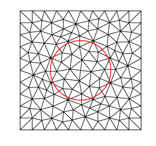
Figure 4. Triangulation for example 1 with mesh size $h=1/5$ (left) / $h=1/10$ (right).

By using a series of quasi-uniform triangular meshes, the $L^{2}$ norm and DG energy norm of the error in the approximation to the exact solution with mesh size $h=1/5,1/10,\ldots,1/80$ are reported in Fig 5. For each fixed $m$, we observe that the errors $\|u-u_{h}\|_{L^{2}(\Omega)}$ and $|\!|\!|u-u_{h}|\!|\!|$ converge to zero at the rate $O(h^{m+1})$ and $O(h^{m})$ as the mesh is refined, respectively. Such convergence rates are consistent with the theoretical results.

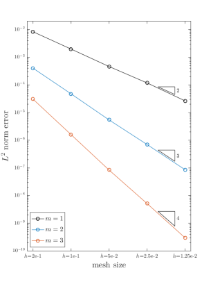
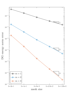
Figure 5. The convergence orders under $L^{2}$ norm (left) / DG energy norm (right) for Example 1.

Example 2.

In this example, we consider the same interface and the same domain as in Example 1. The analytical solution $u(x,y)$ and the coefficient are defined in the same way as in Example 1. But we solve the elliptic interface problem based on a sequence of polygonal meshes as shown in Fig 6, which are generated by PolyMesher [45].

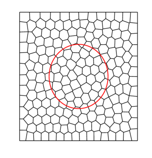
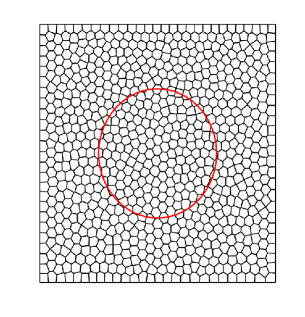
Figure 6. Voronoi mesh for example 2 with 200 elements (left) / 800 elements (right).

The numerically detected convergence orders are displayed in Fig 7 for both error measurements. It is clear that the orders of convergence in $L^{2}$ norm and DG energy norm are $O(h^{m+1})$ and $O(h^{m})$, respectively, which again are in agreement with the theoretical predicts.

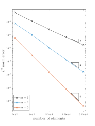
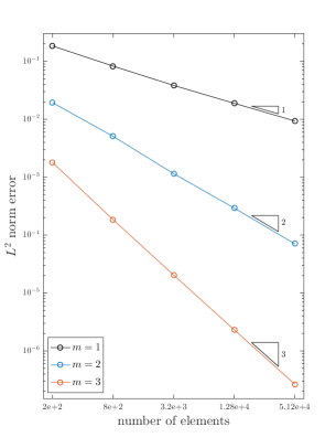
Figure 7. The convergence orders under $L^{2}$ norm (left) / DG energy norm (right) for Example 2.

For the Example 3 - 6, the computational domain is $(-1,1)\times(-1,1)$ and we solve the test problems on a sequence of triangular meshes with mesh size $h=1/5,1/10,\cdots,1/80$.

Example 3.

In this case, we consider the problem in [54] which contains the strongly discontinuous coefficient $\beta$ to test the robustness of the proposed method. We consider the elliptic problem with an ellipse interface (see Fig 8),

$$\phi(x,y)=\left(\frac{x}{18/27}\right)^{2}+\left(\frac{y}{10/27}\right)^{2}-1$$

The exact solution and the coefficient are given as

$$u(x,y) =\begin{cases}5e^{-x^{2}-y^{2}},\quad&\text{outside }\Gamma,\\ e^{x}\cos(y),\quad&\text{inside }\Gamma,\\ \end{cases}$$

$$\beta =\begin{cases}1,\quad&\text{outside }\Gamma,\\ 1000,\quad&\text{inside }\Gamma.\\ \end{cases}$$

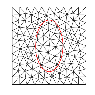
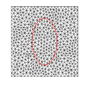
Figure 8. Triangulation for example 3 with mesh size $h=1/5$ (left) / $h=1/10$ (right).

There is a large jump in $\beta$ across the interface $\Gamma$, which may lead to an ill-conditioned linear system. We still use the direct sparse solver to solve the resulting sparse linear system and our method shows the robustness for this case. As can be seen from Fig 9, the computed rates of convergence match with the theoretical analysis.

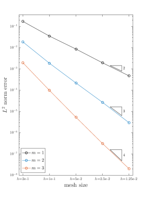
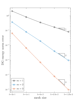
Figure 9. The convergence orders under $L^{2}$ norm (left) / DG energy norm (right) for Example 3.

Example 4.

In this example, we consider solving the elliptic problem with a kidney-shaped interface [25], which is governed by the following level set function

$$\phi(x,y)=\left(2\left(\left(x+0.5\right)^{2}+y\right)-x-0.5\right)^{2}-\left(\left(x+0.5\right)^{2}+y^{2}\right)+0.1.$$

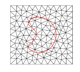
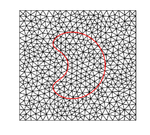
Figure 10. Triangulation for example 4 with mesh size $h=1/5$ (left) / $h=1/10$ (right).

The boundary data and source term are derived from the exact solution and coefficient

$$u(x,y) =\begin{cases}0.1\cos(1-x^{2}-y^{2}),&\quad\text{outside }\Gamma,\\ \sin(2x^{2}+y^{2}+2)+x,&\quad\text{inside }\Gamma,\\ \end{cases}$$

$$\beta =\begin{cases}10,&\quad\text{outside }\Gamma,\\ 1,&\quad\text{inside }\Gamma.\\ \end{cases}$$

We present numerical results in Fig 11 and the predicted convergence rates for both norms are verified.

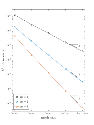
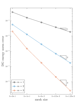
Figure 11. The convergence orders under $L^{2}$ norm (left) / DG energy norm (right) for Example 4.

Example 5.

Next, we consider a standard test case with an interface consisting of both concave and convex curve segments [54]. The interface is parametrized with the polar angle $\theta$

$$r=\frac{1}{2}+\frac{\sin 5\theta}{7}.$$

The exact solution is selected to be

$$u(x,y) =\begin{cases}0.1(x^{2}+y^{2})^{2}-0.01\ln(2\sqrt{x^{2}+y^{2}}),\quad&\text{outside }\Gamma,\\ e^{x^{2}+y^{2}},\quad&\text{inside }\Gamma,\\ \end{cases}$$

$$\beta =\begin{cases}10,\quad&\text{outside }\Gamma,\\ 1,\quad&\text{inside }\Gamma.\\ \end{cases}$$

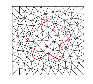
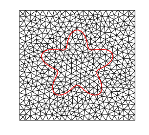
Figure 12. Triangulation for Example 6 with mesh size $h=1/5$ (left) / $h=1/10$ (right).

The convergence of the numerical solutions is displayed in Fig 13. Again we observe optimal rates of convergence for both norms as the mesh size is decreased.

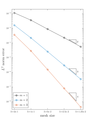
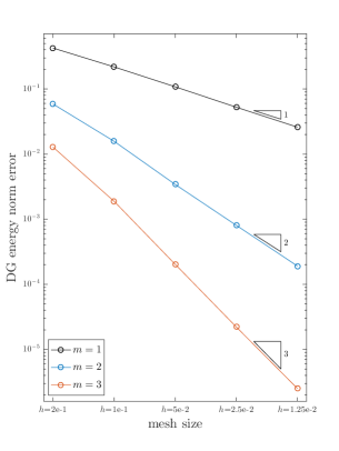
Figure 13. The convergence orders under $L^{2}$ norm (left) / DG energy norm (right) for Example 5.

Example 6.

In this case, we investigate the performance of our proposed method when dealing with the problem with low regularities. The interface can be found in [22], which is governed by the following level set function

$$\phi(x,y)=\begin{cases}y-2x,&\quad x+y>0,\\ y+0.5x,&\quad x+y\leq 0.\\ \end{cases}$$

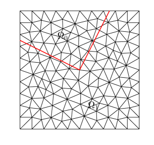
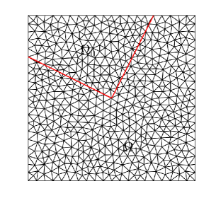
Figure 14. Triangulation for Example 6 with mesh size $h=1/5$ (left) / $h=1/10$ (right).

We note that the interface is only Lipschitz continuous and it has a kink at $(0,0)$, see Fig 14. The analytical solution $u(x,y)$ is given by

$$u(x,y) =\begin{cases}8,&\quad(x,y)\in\Omega_{0},\\ \sin(x+y),&\quad(x,y)\in\Omega_{1}\text{ and }x+y\leq 0,\\ x+y,&\quad(x,y)\in\Omega_{1}\text{ and }x+y>0.\\ \end{cases}$$

We choose $\beta=1$ over the domain $(-1,1)\times(-1,1)$. The solution $u(x,y)$ is $C^{2}$ continuous but not $C^{3}$ continuous across the line $x+y=1$. The numerical errors in terms of $L^{2}$ norm and DG energy norm are gathered in Tab 2. It is observed that when $m=1,2$ the numerical solutions converge optimally with rate $O(h^{m+1})$ for $L^{2}$ norm and $m$ order for DG energy norm, which matches with the fact that the exact solution $u$ belongs to $H^{3}(\Omega_{0}\cup\Omega_{1})$. When $m=3$ the computed orders of convergence in $\|\cdot\|_{L^{2}(\Omega)}$ and $|\!|\!|\cdot|\!|\!|$ are about $O(h^{3.5})$ and $O(h^{2.5})$, respectively. A possible explanation of the convergence orders can be traced to lack of $H^{4}$-regularity of the exact solution on the domain $\Omega_{1}$.

order $m$	$h$	$L^{2}$ error	order	DG error	order
$m=1$	2.00e-1	7.661e-3	-	1.835e-1	-
	1.00e-1	2.515e-3	1.61	5.022e-2	1.00
	5.00e-2	6.498e-4	1.95	2.445e-2	1.03
	2.50e-2	1.653e-4	1.97	1.199e-2	1.02
	1.25e-2	4.202e-5	1.98	1.156e-2	1.00
$m=2$	2.00e-1	4.727e-4	-	9.283e-3	-
	1.00e-1	6.423e-5	2.85	2.393e-3	1.95
	5.00e-2	7.249e-6	3.16	5.872e-4	2.01
	2.50e-2	9.171e-7	2.98	1.505e-4	1.97
	1.25e-2	1.126e-7	3.02	6.401e-5	2.02
$m=3$	2.00e-1	1.229e-4	-	3.145e-3	-
	1.00e-1	1.126e-5	3.45	3.361e-4	2.41
	5.00e-2	9.603e-7	3.55	5.721e-5	2.53
	2.50e-2	8.249e-8	3.55	1.816e-5	2.55
	1.25e-2	6.999e-9	3.56	3.108e-6	2.55

Table 2. The convergence orders under $L^{2}$ norm and DG energy norm for Example 6.

4.2. 3D Example

Example 7.

Here we consider a three-dimensional elliptic interface problem. The domain $\Omega$ is $(0,1)^{3}$ and the spherical interface is given by

$$\phi(x,y,z)=(x-0.5)^{2}+(y-0.5)^{2}+(z-0.5)^{2}-r^{2},$$

with radius $r=0.35$. We select $\beta=1$ in the whole domain and the exact solution is taken as

$$u(x,y,z)=\begin{cases}\sin(\pi x)\sin(\pi y)\sin(\pi z),\quad&\text{outside $\Gamma$},\\ e^{x^{2}+y^{2}+z^{2}},\quad&\text{inside $\Gamma$}.\\ \end{cases}$$

We adopt a family of tetrahedral meshes with mesh size $h=1/4$, $1/8$, $1/16$, $1/32$ to solve the interface problem (see Fig 15). The numerical solutions on the meshes with $h=1/16$ and $h=1/32$ are depicted in Fig 16 and these two solutions are obtained with the accuracy $m=3$. We display the slices at $y=0.5$ and $z=0.5$ of the numerical approximations on both meshes and both solutions significantly involve a discontinuity across a spherical, which are accordant with the interface. The convergence rates under both norms are shown in Fig 17. Clearly, the numerical results are still consistent with our theoretical predictions.

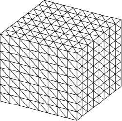
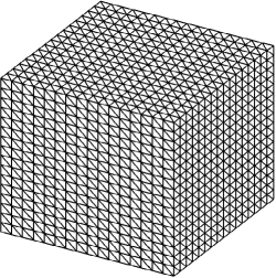
Figure 15. Tetrahedral meshes for example 7 with mesh size $h=1/8$ (left) / $h=1/16$ (right).

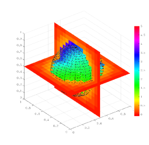
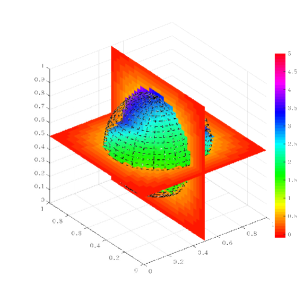
Figure 16. The numerical solution on the tetrahedral mesh with mesh size $h=1/16$ (left) / $h=1/32$ (right).

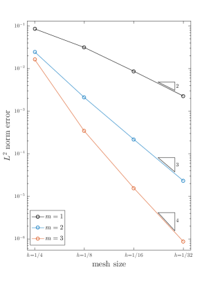
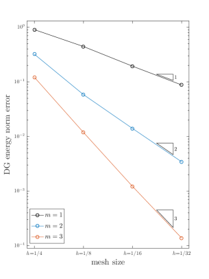
Figure 17. The convergence orders under $L^{2}$ norm (left) / DG energy norm (right) for Example 7.

Example 8.

In this example, we consider a three-dimensional elliptic problem [49] with a smooth interface that is governed by the following level set function (see Fig 18),

$$\phi(x,y,z)=\left((2.5(x-0.5))^{2}+(4.2(y-0.5))^{2}+(2.5(z-0.5))^{2}+0.9\right)^{2}-64(y-0.5)^{2}-1.3.$$

The exact solution is choose to be

$$u(x,y,z)=\begin{cases}\cos(\pi x)\cos(\pi y)\cos(\pi z),\quad&\text{outside $\Gamma$},\\ 5e^{x^{2}+y^{2}+z^{2}},\quad&\text{inside $\Gamma$}.\\ \end{cases}$$

The domain $\Omega$ is taken to be $(0,1)^{3}$ and the coefficient $\beta$ is fixed as $1$. We also use the tetrahedral meshes with mesh size $h=1/4$, $1/8$, $1/16$, $1/32$ for solving the problem (see Fig 15). The slices of the numerical solution with the accuracy $m=3$ on the tetrahedral mesh with $h=1/32$ at $x=0.5$ and at $z=0.5$ are depicted in Fig 19. It is clear that the discontinuity of the numerical solution sketches a curve which matches with the interface given by the level set function (see 18). We also display the convergence history of the numerical approximation under both $L^{2}$ norm and DG energy norm in Fig 20. The convergence rate of $L^{2}$ error may seem less than the predicted value when the accuracy $m=1$. The rate is gradually more close to the theoretical value and we may expect the rate would go back to $O(h^{2})$ as the mesh size tends to zero. For $m=2$ and $m=3$, the computed convergence rates under both error measurements are in agreement with the theoretical results.

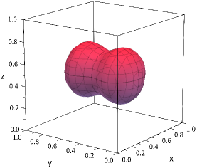
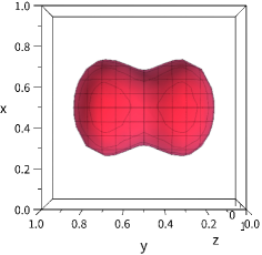
Figure 18. The interface of Example 8.

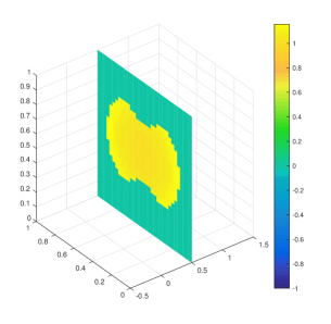
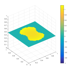
Figure 19. The slice of the numerical solution at $x=0.5$ (left) / at $z=0.5$ (right).

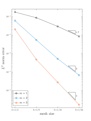
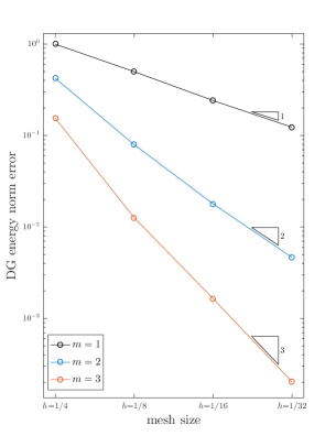
Figure 20. The convergence orders under $L^{2}$ norm (left) / DG energy norm (right) for Example 8.

4.3. Integrals on Cut Element

In our method, computing the following types of integrals defined on the cut element is an important issue,

$$\int_{K^{0}}v(\boldsymbol{x})\mathrm{d}\boldsymbol{x},\quad\int_{K^{1}}v(\boldsymbol{x})\mathrm{d}\boldsymbol{x},\quad\int_{\Gamma_{K}}v(\boldsymbol{x})\mathrm{d}\boldsymbol{s},$$

where $K\in\mathcal{T}_{h}^{\Gamma}$ is a cut element and $K^{0}=K\cap\Omega_{0}$, $K^{1}=K\cap\Omega_{1}$ and $\Gamma_{K}=K\cap\Gamma$. Here we list two numerical methods for computing these integrals. The first is we generate highly accurate quadrature points and weights corresponding to the domain $K^{0}$, $K^{1}$ and the interface $\Gamma_{K}$. We refer to [15, 39, 23] for some approaches about finding such quadrature points and weights. The computational cost of the first method is much more expensive than ordinary numerical quadrature methods. The second one is we approximate the interface $\Gamma_{K}$ by planes or lines inside the element $K$, see Fig  21 for an example. In this case, we only need to generate quadrature points and weights for polygons or polyhedrons. The computational cost is much less than the first method but the result is less accurate. We refer to [47] for more details about this method.

Here we make a comparison between two methods. We solve the Example 7 by both two numerical quadrature methods. We call the C subroutines in PHG package [52, 15] to generate highly accurate quadrature points and weights for the cut tetrahedrons. For the second methods and for element $K\in\mathcal{T}_{h}^{\Gamma}$, we let $K^{0}$ be approximated by $\widetilde{K}^{0}$ and let $K^{1}$ be approximated by $\widetilde{K}^{1}$. The actual computational domains $\widetilde{\Omega}_{0}$ and $\widetilde{\Omega}_{1}$ are then given as

$$\widetilde{\Omega}_{i}=\left(\bigcup_{K\in\mathcal{T}_{h}^{\Gamma}}\widetilde{K}^{i}\right)\bigcup\left(\bigcup_{K\in\mathcal{T}_{h}^{i}\backslash\mathcal{T}_{h}^{\Gamma}}K\right),\quad i=0,1.$$

We list the $L^{2}$ errors $\|u-u_{h}^{1}\|_{L^{2}(\Omega_{0}\cup\Omega_{1})}$ and $\|u-u_{h}^{2}\|_{L^{2}(\widetilde{\Omega}_{0}\cup\widetilde{\Omega}_{1})}$ in Tab 3, where $u_{h}^{1}$ and $u_{h}^{2}$ are the numerical solutions obtained by the first and second numerical quadrature methods, respectively. From Tab 3, we observe that the two errors are gradually closer to each other when the mesh size tends to zero. We note that both quadrature methods work in our numerical scheme and the first one is more accurate but much more computational cost is required.

		$h=1/4$	$h=1/8$	$h=1/16$	$h=1/32$
$m=1$	$\|u-u_{h}^{1}\|_{L^{2}(\Omega_{0}\cup\Omega_{1})}$	7.1514e-2	3.0977e-2	1.0696e-2	2.8099e-3
	$\|u-u_{h}^{2}\|_{L^{2}(\widetilde{\Omega}_{0}\cup\widetilde{\Omega}_{1})}$	1.0216e-1	3.3384e-2	1.1173e-2	2.8274e-3
$m=2$	$\|u-u_{h}^{1}\|_{L^{2}(\Omega_{0}\cup\Omega_{1})}$	6.1523e-2	2.0271e-3	1.8898e-4	2.3557e-5
	$\|u-u_{h}^{2}\|_{L^{2}(\widetilde{\Omega}_{0}\cup\widetilde{\Omega}_{1})}$	3.4460e-2	2.4149e-3	2.1523e-4	2.3799e-5
$m=3$	$\|u-u_{h}^{1}\|_{L^{2}(\Omega_{0}\cup\Omega_{1})}$	5.1865e-2	3.9632e-4	1.7698e-5	9.0215e-7
	$\|u-u_{h}^{2}\|_{L^{2}(\widetilde{\Omega}_{0}\cup\widetilde{\Omega}_{1})}$	1.7197e-2	3.7255e-4	1.5553e-5	8.7805e-7

Table 3. The $L^{2}$ errors $\|u-u_{h}^{1}\|_{L^{2}(\Omega_{0}\cup\Omega_{1})}$ and $\|u-u_{h}^{2}\|_{L^{2}(\widetilde{\Omega}_{0}\cup\widetilde{\Omega}_{1})}$.

Figure 21. The interface inside a cut element $K$ for $d=3$ (left) / $d=2$ (right).

4.4. Efficiency comparison

Hughes et al. [24] point out that the number of unknowns of a discretized problem is a proper indicator for the efficiency of a numerical method. To show the efficiency in DOFs of our method, we make a comparison among the unfitted DG method [37], the unfitted penalty finite element method [50, 51] and our method by solving the two-dimensional elliptic interface problem. The first method adopts the standard discontinuous finite element space, and the second method employs the traditional continuous finite element space. The solution and the partition are taken from Example 1. In Fig 22, we plot the $L^{2}$ norm of the error of three methods against the number of degrees of freedom with $1\leq m\leq 3$.

One see that for the low orders of approximation($m=1$), the penalty FE method is the most efficient method. For $m=2$, our method shows almost the same efficiency as the penalty FE method. For the high order accuracy($m=3$), our method performs better than the other methods.

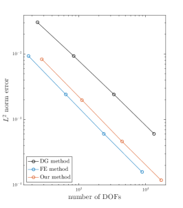
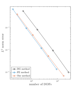
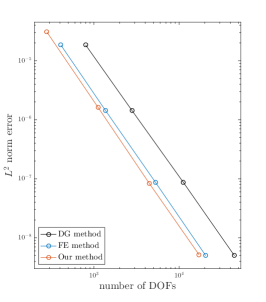
Figure 22. Comparison of the $L^{2}$ errors in number of DOFs by three methods with $m=1$, $2$, and $3$.

5. Conclusion

We proposed a new discontinuous Galerkin method for elliptic interface problem. The approximation space is constructed by solving the local least squares problem. We proved optimal convergence orders in both $L^{2}$ norm and DG energy norm. A series of numerical results confirm our theoretical results and exhibit the flexibility, robustness and efficiency of the proposed method.

Appendix A Construction of Element Patch

Here we present the algorithm to the construction of the element patch in Alg  1 and we also give some an example of constructing element patches. We consider a circular interface. Let $\Omega_{1}$ be the domain inside the circle and $\Omega_{0}=\Omega\backslash\Omega_{1}$. For element $K\in\mathcal{T}_{h}^{0}\backslash\mathcal{T}_{h}^{\Gamma}$, the construction of $S^{0}(K)$ is presented in Fig 24.

.

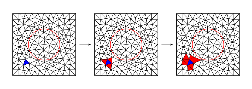
Figure 23. Example to build element patch $S^{0}(K)$ for $K\in\mathcal{T}_{h}^{0}\backslash\mathcal{T}_{h}^{\Gamma}$.

For element $K\in\mathcal{T}_{h}^{1}\backslash\mathcal{T}_{h}^{\Gamma}$, the construction of $S^{1}(K)$ is presented in Fig 24.

.

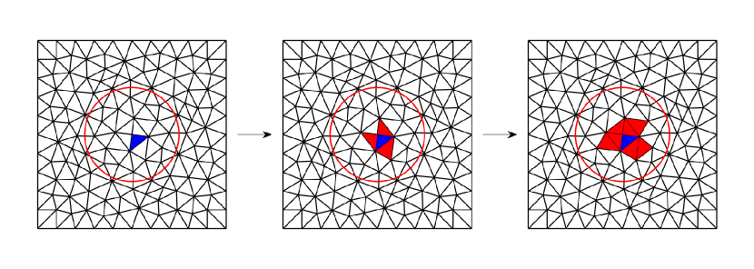
Figure 24. Example to build element patch $S^{1}(K)$ for $K\in\mathcal{T}_{h}^{1}\backslash\mathcal{T}_{h}^{\Gamma}$.

Algorithm 1 Construction of Element Patch

0:  partition $\mathcal{T}_{h}$ and a uniform threshold $\#S(K)$;

0:  the element patches $S^{0}(K)$ for all $K$ in $\mathcal{T}_{h}^{0}$ and the element patches $S^{1}(K)$ for all $K$ in $\mathcal{T}_{h}^{1}$;

1:  for $i\in\{0,1\}$ do

2:     for each $K\in\mathcal{T}_{h}^{i}\backslash\mathcal{T}_{h}^{\Gamma}$ do

3:        set $t=0$, $S_{t}^{i}(K)=\left\{K\right\}$;

4:        while the cardinality of $S_{t}^{i}(K)$ $<$ $\#S(K)$ do

5:           initialize the set $S_{t+1}^{i}(K)=S_{t}^{i}(K)$;

6:           for each $K\in S_{t}^{i}(K)$ do

7:              let $N(K)$ be the face-neighbouring elements of $K$;

8:              for each $\widetilde{K}\in N(K)$ do

9:                 if $\widetilde{K}\notin S_{t+1}^{i}(K)$ and $\widetilde{K}\in\mathcal{T}_{h}^{i}$ then

10:                    add $\widetilde{K}$ to $S_{t+1}^{i}(K)$;

11:                 end if

12:                 if the cardinality of $S_{t}^{i}(K)$ = $\#S(K)$ then

13:                    break while;

14:                 end if

15:              end for

16:           end for

17:           let $t=t+1$;

18:        end while

19:        let $S^{i}(K)=S_{t}^{i}(K)$;

20:     end for

21:  end for

22:  for each $K\in\mathcal{T}_{h}^{\Gamma}$ do

23:     seek $K_{\circ}^{0}$ and $K_{\circ}^{1}$ and let $S^{0}(K)=S^{0}(K_{\circ}^{0})$ and $S^{1}(K)=S^{1}(K_{\circ}^{1})$;

24:  end for

Appendix B 1D Example

Here we present a one-dimensional example to illustrate our method. We consider the interval $\Omega=[-1,1]$ which is divided into two parts $\Omega_{0}=(-1,-0.2)$ and $\Omega_{1}=(-0.2,1)$. We partition $\Omega$ into 8 elements $\left\{K_{1},K_{2},\cdots,K_{8}\right\}$ with uniform spacing.

Figure 25. The uniform grid on $[-1,1]$.

$\left\{x_{1},x_{2},\cdots,x_{8}\right\}$ are the set of collocations where $x_{i}$ is the midpoint of the element $K_{i}$. Since $\mathcal{T}_{h}^{\Gamma}=\left\{K_{4}\right\}$, we construct element patches for elements in $\mathcal{T}_{h}^{\backslash\Gamma}$. The element patches could be constructed as

$$S^{0}(K_{1})=\left\{K_{1},K_{2}\right\},\quad S^{0}(K_{2})=\left\{K_{2},K_{3}\right\},\quad S^{0}(K_{3})=\left\{K_{2},K_{3},K_{4}\right\},$$

$$S^{1}(K_{5}) =\left\{K_{4},K_{5},K_{6}\right\},\quad S^{1}(K_{6})=\left\{K_{5},K_{6},K_{7}\right\},$$

$$S^{1}(K_{7}) =\left\{K_{6},K_{7}\right\},\quad S^{1}(K_{8})=\left\{K_{7},K_{8}\right\}.$$

Then for element $K_{4}$ it is clear that $K_{\circ}^{0}=K_{3}$ and $K_{\circ}^{1}=K_{5}$, and the element patches of $K_{4}$ are

$$S^{0}(K_{4}) =S^{0}(K_{3})=\left\{K_{2},K_{3},K_{4}\right\},$$

$$S^{1}(K_{4}) =S^{1}(K_{5})=\left\{K_{4},K_{5},K_{6}\right\}.$$

Then we would solve the least squares problem on every patch. We take $S^{0}(K_{3})$ for an example, for a continuous function $g$ and $m=1$ the least squares problem is written as

$$\mathop{\arg\min}_{(a,b)\in\mathbb{R}}\sum_{i=2}^{4}|(ax_{i}+b)-g(x_{i})|^{2}.$$

It is easy to get the unique solution

$$(a,b)^{T}=(A^{T}A)^{-1}A^{T}q,$$

where

$$A=\begin{bmatrix}1&x_{2}\\ 1&x_{3}\\ 1&x_{4}\\ \end{bmatrix},\qquad q=\begin{bmatrix}g(x_{2})\\ g(x_{3})\\ g(x_{4})\\ \end{bmatrix}.$$

We note that the matrix $(A^{T}A)^{-1}A^{T}$ has no relationship to the function $g$ and contains all information of all $\lambda_{K}^{i}$ on element $K_{2}$. Hence we store the matrix $(A^{T}A)^{-1}A^{T}$ for every element patch to represent all $\lambda_{K}^{i}$. It is in the same way when we deal with the high dimensional problem.

References

[1]
R. A. Adams and J. J. F. Fournier, Sobolev Spaces, second ed., Pure
and Applied Mathematics (Amsterdam), vol. 140, Elsevier/Academic Press,
Amsterdam, 2003.
[2]
S. Adjerid, N. Chaabane, and T. Lin, An immersed discontinuous finite
element method for Stokes interface problems, Comput. Methods Appl. Mech.
Engrg. 293 (2015), 170–190.
[3]
N. An and H. Chen, A partially penalty immersed interface finite element
method for anisotropic elliptic interface problems, Numer. Methods Partial
Differential Equations 30 (2014), no. 6, 1984–2028.
[4]
P. F. Antonietti, L. Beirão da Veiga, and M. Verani, A mimetic
discretization of elliptic obstacle problems, Math. Comp. 82
(2013), no. 283, 1379–1400.
[5]
I. Babuška, The finite element method for elliptic equations with
discontinuous coefficients, Computing 5 (1970), no. 3, 207–213.
[6]
J. W. Barrett and C. M. Elliott, Fitted and unfitted finite-element
methods for elliptic equations with smooth interfaces, IMA J. Numer. Anal.
7 (1987), no. 3, 283–300.
[7]
T. Belytschko and T. Black, Elastic crack growth in finite elements with
minimal remeshing, Internat. J. Numer. Methods Engrg. 45 (1999),
no. 5, 601–620.
[8]
E. Burman and A. Ern, An unfitted hybrid high-order method for elliptic
interface problems, SIAM J. Numer. Anal. 56 (2018), no. 3,
1525–1546.
[9]
A. Cangiani, E. H. Georgoulis, and Y. A. Sabawi, Adaptive discontinuous
Galerkin methods for elliptic interface problems, Math. Comp. 87
(2018), no. 314, 2675–2707.
[10]
W. Cao, X. Zhang, Z. Zhang, and Q. Zou, Superconvergence of immersed
finite volume methods for one-dimensional interface problems, J. Sci.
Comput. 73 (2017), no. 2-3, 543–565.
[11]
T. Chen and J. Strain, Piecewise-polynomial discretization and
Krylov-accelerated multigrid for elliptic interface problems, J. Comput.
Phys. 227 (2008), no. 16, 7503–7542.
[12]
Z. Chen and J. Zou, Finite element methods and their convergence for
elliptic and parabolic interface problems, Numer. Math. 79 (1998),
no. 2, 175–202.
[13]
C.-C. Chu, I. G. Graham, and T.-Y. Hou, A new multiscale finite element
method for high-contrast elliptic interface problems, Math. Comp.
79 (2010), no. 272, 1915–1955.
[14]
P. G. Ciarlet, The Finite Element Method for Elliptic Problems,
Classics in Applied Mathematics, vol. 40, Society for Industrial and Applied
Mathematics (SIAM), Philadelphia, PA, 2002, Reprint of the 1978 original
[North-Holland, Amsterdam; MR0520174 (58 #25001)].
[15]
T. Cui, W. Leng, H. Liu, L. Zhang, and W. Zheng, High-order numerical
quadratures in a tetrahedron with an implicitly defined curved interface,
ACM Trans. Math. Softw. (2019), to appear.
[16]
R. P. Fedkiw, T. Aslam, B. Merriman, and S. Osher, A non-oscillatory
Eulerian approach to interfaces in multimaterial flows (the ghost fluid
method), J. Comput. Phys. 152 (1999), no. 2, 457–492.
[17]
R. Guo and T. Lin, A higher degree immersed finite element method based
on a Cauchy extension for elliptic interface problems, SIAM J. Numer.
Anal. 57 (2019), no. 4, 1545–1573.
[18]
G. Guyomarc’h, C.-O. Lee, and K. Jeon, A discontinuous Galerkin method
for elliptic interface problems with application to electroporation, Comm.
Numer. Methods Engrg. 25 (2009), no. 10, 991–1008.
[19]
J. Guzmán, M. A. Sánchez, and M. Sarkis, A finite element method
for high-contrast interface problems with error estimates independent of
contrast, J. Sci. Comput. 73 (2017), no. 1, 330–365.
[20]
A. Hansbo and P. Hansbo, An unfitted finite element method, based on
Nitsche’s method, for elliptic interface problems, Comput. Methods Appl.
Mech. Engrg. 191 (2002), no. 47-48, 5537–5552.
[21]
S. Hou and X.-D. Liu, A numerical method for solving variable coefficient
elliptic equation with interfaces, J. Comput. Phys. 202 (2005),
no. 2, 411–445.
[22]
S. Hou, W.g Wang, and L. Wang, Numerical method for solving matrix
coefficient elliptic equation with sharp-edged interfaces, J. Comput. Phys.
229 (2010), no. 19, 7162–7179.
[23]
P. Huang, H. Wu, and Y. Xiao, An unfitted interface penalty finite
element method for elliptic interface problems, Comput. Methods Appl. Mech.
Engrg. 323 (2017), 439–460.
[24]
T. J. R. Hughes, G. Engel, L. Mazzei, and M. G. Larson, A comparison of
discontinuous and continuous Galerkin methods based on error estimates,
conservation, robustness and efficiency, Discontinuous Galerkin methods
(Newport, RI, 1999), Lect. Notes Comput. Sci. Eng., vol. 11, Springer,
Berlin, 2000, pp. 135–146.
[25]
L. N. T. Huynh, N. C. Nguyen, J. Peraire, and B. C. Khoo, A high-order
hybridizable discontinuous Galerkin method for elliptic interface
problems, Internat. J. Numer. Methods Engrg. 93 (2013), no. 2,
183–200.
[26]
R. B. Kellogg, Higher order singularities for interface problems, The
mathematical foundations of the finite element method with applications to
partial differential equations (Proc. Sympos., Univ. Maryland,
Baltimore, Md., 1972), 1972, pp. 589–602. MR 0433926
[27]
by same author, On the Poisson equation with intersecting interfaces,
Applicable Anal. 4 (1974/75), 101–129.
[28]
R. J. LeVeque and Z. Li, The immersed interface method for elliptic
equations with discontinuous coefficients and singular sources, SIAM J.
Numer. Anal. 31 (1994), no. 4, 1019–1044.
[29]
R. Li, P. Ming, Z. Sun, F. Yang, and Z. Yang, A discontinuous Galerkin
method by patch reconstruction for biharmonic problem, J. Comput. Math.
37 (2019), no. 4, 563–580.
[30]
R. Li, P. Ming, Z. Sun, and Z. Yang, An arbitrary-order discontinuous
Galerkin method with one unknown per element, J. Sci. Comput. 80
(2019), no. 1, 268–288.
[31]
R. Li, P. Ming, and F. Tang, An efficient high order heterogeneous
multiscale method for elliptic problems, Multiscale Model. Simul.
10 (2012), no. 1, 259–283.
[32]
Z. Li, The immersed interface method using a finite element formulation,
Appl. Numer. Math. 27 (1998), no. 3, 253–267.
[33]
Z. Li and K. Ito, The immersed interface method, Frontiers in Applied
Mathematics, vol. 33, Society for Industrial and Applied Mathematics (SIAM),
Philadelphia, PA, 2006, Numerical solutions of PDEs involving interfaces and
irregular domains.
[34]
T. Lin, Y. Lin, and X. Zhang, Partially penalized immersed finite element
methods for elliptic interface problems, SIAM J. Numer. Anal. 53
(2015), no. 2, 1121–1144.
[35]
X.-D. Liu, R. P. Fedkiw, and M. Kang, A boundary condition capturing
method for Poisson’s equation on irregular domains, J. Comput. Phys.
160 (2000), no. 1, 151–178.
[36]
A. Massing, M. G. Larson, A. Logg, and M. E. Rognes, A stabilized
Nitsche fictitious domain method for the Stokes problem, J. Sci. Comput.
61 (2014), no. 3, 604–628.
[37]
R. Massjung, An unfitted discontinuous Galerkin method applied to
elliptic interface problems, SIAM J. Numer. Anal. 50 (2012), no. 6,
3134–3162.
[38]
A. Mayo, Fast high order accurate solution of Laplace’s equation on
irregular regions, SIAM J. Sci. Statist. Comput. 6 (1985), no. 1,
144–157.
[39]
B. Müller, F. Kummer, and M. Oberlack, Highly accurate surface and
volume integration on implicit domains by means of moment-fitting, Internat.
J. Numer. Methods Engrg. 96 (2013), no. 8, 512–528.
[40]
M. Oevermann and R. Klein, A Cartesian grid finite volume method for
elliptic equations with variable coefficients and embedded interfaces, J.
Comput. Phys. 219 (2006), no. 2, 749–769.
[41]
C. S. Peskin, Numerical analysis of blood flow in the heart, J. Comput.
Phys. 25 (1977), no. 3, 220–252.
[42]
M. Petzoldt, Regularity results for Laplace interface problems in two
dimensions, Z. Anal. Anwendungen 20 (2001), no. 2, 431–455.
[43]
M. J. D. Powell, Approximation theory and methods, Cambridge University
Press, Cambridge-New York, 1981.
[44]
J. A. Roĭtberg and Z. G. Šeftel, A homeomorphism theorem for
elliptic systems, and its applications, Mat. Sb. (N.S.) 78 (120)
(1969), 446–472.
[45]
C. Talischi, G. H. Paulino, A. Pereira, and I. F. M. Menezes, PolyMesher: a general-purpose mesh generator for polygonal elements
written in Matlab, Struct. Multidiscip. Optim. 45 (2012), no. 3,
309–328.
[46]
E. Wadbro, S. Zahedi, G. Kreiss, and M. Berggren, A uniformly
well-conditioned, unfitted Nitsche method for interface problems, BIT
53 (2013), no. 3, 791–820.
[47]
L. Wang, S. Hou, and L. Shi, An improved non-traditional finite element
formulation for solving three-dimensional elliptic interface problems,
Comput. Math. Appl. 73 (2017), no. 3, 374–384.
[48]
X. S. Wang, L.T. Zhang, and W. K. Liu, On computational issues of
immersed finite element methods, J. Comput. Phys. 228 (2009),
no. 7, 2535–2551.
[49]
Z. Wei, C. Li, and S. Zhao, A spatially second order alternating
direction implicit (ADI) method for solving three dimensional parabolic
interface problems, Comput. Math. Appl. 75 (2018), no. 6,
2173–2192.
[50]
H. Wu and Y. Xiao, An unfitted -interface penalty finite element
method for elliptic interface problems, J. Comput. Math. 37 (2019),
no. 3, 316–339.
[51]
Y. Xiao, J. Xu, and F. Wang, High-order extended finite element methods
for solving interface problems, Comput. Methods Appl. Mech. Engrg.
364 (2020), 112964, 21.
[52]
J. Xu, Y. Xie, and B. Lu, A parallel finite element solver for
biomolecular simulations based on the toolbox PHG, J. Numer. Methods
Comput. Appl. 37 (2016), no. 1, 67–82,
https://lsec.cc.ac.cn/phg/download.htm.
[53]
S. Yu, Y. Zhou, and G. W. Wei, Matched interface and boundary (MIB)
method for elliptic problems with sharp-edged interfaces, J. Comput. Phys.
224 (2007), no. 2, 729–756.
[54]
Y. C. Zhou and G. W. Wei, On the fictitious-domain and interpolation
formulations of the matched interface and boundary (MIB) method, J.
Comput. Phys. 219 (2006), no. 1, 228–246.
[55]
O. C. Zienkiewicz, R. L. Taylor, S. J. Sherwin, and J. Peiró, On
discontinuous Galerkin methods, Internat. J. Numer. Methods Engrg.
58 (2003), no. 8, 1119–1148.